The variability of optical Fe ii emission in PG QSO 1700+518

Abstract

It is found that Fe ii emission contributes significantly to the optical and ultraviolet spectra of most active galactic nuclei. The origin of the optical/UV Fe ii emission is still a question open to debate. The variability of Fe ii would give clues to this origin. Using 7.5 yr spectroscopic monitoring data of one Palomer-Green (PG) quasi-stellar object (QSO), PG 1700+518, with strong optical Fe ii emission, we obtain the light curves of the continuum $f_{\lambda}(5100\AA)$ , Fe ii , the broad component of H$\beta$ , and the narrow component of H$\beta$ by the spectral decomposition. Through the interpolation cross-correlation method, we calculate the time lags for light curves of Fe ii , the total H$\beta$ , the broad component of H$\beta$ , and the narrow component of H$\beta$ with respect to the continuum light curve. We find that the Fe ii time lag in PG1700+518 is $209^{+100}_{-147}$ days, and the H$\beta$ time lag cannot be determined. Assuming that Fe ii and H$\beta$ emission regions follow the virial relation between the time lag and the FWHM for the H$\beta$ and Fe ii emission lines, we can derive that the H$\beta$ time lag is $148^{+72}_{-104}$ days. The H$\beta$ time lag calculated from the empirical luminosity–size relation is 222 days, which is consistent with our measured Fe ii time lag. Considering the optical Fe ii contribution, PG 1700+518 shares the same characteristic on the spectral slope variability as other 15 PG QSOs in our previous work, i.e., harder spectrum during brighter phase.

1. Introduction

The variability is a common phenomenon in quasi-stellar objects (QSOs) and provides a powerful constraint on their central engines. In the past two decades, the optical variability research focused on the spectral monitoring instead of the pure photometric monitoring. With the active galactic nuclei (AGNs) watch and the Palomer-Green (PG) QSOs spectrophotometrical monitoring projects, the reverberation mapping method, i.e., exploring the correlation between the emission lines and the continuum variations, is used to investigate the inner structure in AGNs (e.g., Blandford et al., 1982; Peterson, 1993). It is found that motions of clouds in the broad line regions (BLRs) are virialized (e.g., Kaspi et al., 2000, 2005; Peterson et al., 2004). With the line width of H$\beta$ , Mg ii , C iv from BLRs, the empirical size-luminosity relation derived from the mapping method is used to calculate the masses of their central supermassive black holes (SMBHs; e.g., Kaspi et al., 2000; McLure & Jarvis, 2004; Bian & Zhao, 2004; Peterson et al., 2004; Greene & Ho, 2005).

It is found that the Fe ii emission contributes significantly to the optical and ultraviolet spectra of most AGNs. Thousands of UV Fe ii emission lines blend together to form a pseudocontinuum, resulting in the “small blue bump” around 3000Å when they are combined with Balmer continuum emission (e.g., Wills et al., 1985). The optical Fe ii would lead to two bumps in two sides around the H$\beta$ $\lambda 4861$Å (e.g., Boroson & Green, 1992). It is found that the flux ratio of Fe ii to H$\beta$ , $R_{\rm Fe}$, where the optical Fe ii flux is the flux of the Fe ii  emission between $\lambda$4434 and $\lambda$4684, strongly correlates with the so-called Eigenvector 1, which is suggested to be driven by the accretion rate (e.g., Boroson & Green, 1992; Marziani et al., 2003a).

The origin of the optical/UV Fe ii emission is still an open question. It is found that photoionized BLRs cannot produce the observed shape and strength of the optical Fe ii emission and that the strength of UV Fe ii cannot be explained unless considering the micro-turbulence of hundreds of km s^-1 or the collisional excitation in warm, dense gas (Baldwin et al., 2004). However, Vestergaard & Peterson (2005) found the correlation between the optical Fe ii variance and the continuum variance and suggested that the optical Fe ii is due to the line fluorescent in a photoionized plasma. It suggests that the optical Fe ii line do not come from the same region as the UV Fe ii emission (e.g., Kuehn et al., 2008). Maoz et al. (1993) found that the reverberation time lag of UV Fe ii in NGC 5548 is about 10 days, similar to C iv time lag, smaller than the H$\beta$ time lag. The reverberation measurement for the optical Fe ii emission has not fared so well. Some suggested that the optical emission is produced in the same region as the other broad emission lines, and some suggested that it is in the outer portion of the BLRs because of narrower FWHM of Fe ii with respect to H$\beta$ (e.g., Laor et al., 1997; Marziani et al., 2003a; Vestergaard & Peterson, 2005; Kuehn et al., 2008). Recently, Hu et al. (2008a, b) did a systematic analysis of Fe ii emission in QSOs from the Sloan Digital Sky Survey (SDSS), and found that the Fe ii emission is redshifted with respect to the rest frame defined by the [O iii] narrow emission line and H$\beta$ intermediate-width component is correlated with Fe ii which locates at the outer portion of the BLRs.

Kaspi et al. (2000) gave the 7.5 yr spectroscopic monitoring data for 17 PG QSOs. There is one PG QSO, PG 1700+518, with strongest optical Fe ii emission and $R_{\rm Fe}=1.42$ (Turnshek et al., 1985; Boroson & Green, 1992). Its H$\beta$ FWHM is $1846\pm 682{\rm km\ s}^{-1}$ (Peterson et al., 2004), and it is also called as a narrow line Seyfert 1 galaxy (NLS1). Using the Fe ii template from one NLS1, I ZW 1, we model the Fe ii emission to investigate the Fe ii variability and the relation to the continuum variability in PG 1700+518. The data and analysis are described in Section 2, the results are given in Section 3, the discussion is given in Section 4, and the conclusions are presented in Section 5. All of the cosmological calculations in this paper assume $H_{\rm 0}=70{\rm km\ s}^{-1}\rm~{}Mpc^{-1}$, $\Omega_{\rm M}=0.3$, $\Omega_{\Lambda}=0.7$.

2. The data and analysis

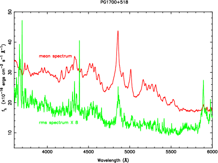
Figure 1.— Mean spectrum (the red curve) and rms spectrum (the green curve; multiplied by 8) for PG 1700+518.

The spectroscopic monitoring data of PG 1700+518 cover 7.5 years from 1991 to 1998, which were done every 1–4 months by using 2.3 m telescope at the Steward Observatory and 1 m telescope at the Wise Observatory. The total number of optical spectra for PG 1700+518 is 39. The observational wavelength coverage is from $\sim$ 4000 to $\sim$ 8000 Å with a spectral resolution of $\sim$ 10Å. Spectra were calibrated to an absolute flux scale using simultaneous observations of nearby standard stars (Kaspi et al., 2000). The 39 spectra of PG 1700+518 are available on the Web site .

In order to check its spectral variance, we calculate its mean and rms spectra (Kaspi et al., 2000; Peterson et al., 2004). In Figure 1, the mean spectrum (the red curve) shows strong optical Fe ii emission, and the rms spectrum (the green curve) shows variable emission for H$\beta$ $\lambda 4861$, He i $\lambda 5878$, and Fe ii (the blueward and redward of H$\beta$ $\lambda 4861$). In the rms spectrum, we can find Fe ii features at $\sim$ 4500Å, 4924Å and 5018Å, suggesting variable Fe ii . The part of Fe ii emission between 4430Å and 4770Å in the rms spectrum is obvious than that between 5080 Å and 5550Å. It is due to the variable continuum slope, more variable in blueward of the spectrum. It is consistent with harder spectrum during bright phase (Pu et al., 2006, Figure 6). In the rms spectrum, we also find weak He ii $\lambda 4686$.

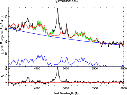
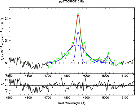
Figure 2.— Example spectral decomposition for PG 1700+518. In the top panel, the black curve is the observed spectrum after the corrections of Galactic-extinction and the redshift, the red line is the sum of the power-law continuum and Fe ii multiples (blue curves). The green ranges are our fitting windows. The bottom panel is the multi-Gaussian fits for the H$\beta$ and [O iii] lines. The red line is the sum of all multi-Gaussian (blue curves). The green curve is our fitting range of the pure H$\beta$ and [O iii] emissions after the subtraction of the power-law continuum and Fe ii multiples.

We use following steps to do the spectral decomposition, which have been used to analyze the spectra for a large QSOs sample from SDSS (Hu et al., 2008a; Bian et al., 2008).

(1) First, the observed spectra are corrected for the Galactic extinction using $A_{V}=0.116$ from the NASA/IPAC Extragalactic Database (NED), assuming an extinction curve of Cardelli, Clayton & Mathis (1989; IR band) and O’Donnell (1994; optical band) with $R_{V}=3.1$. Then the spectra are transformed into the rest frame by the redshift of $0.292$.

(2) The optical and ultraviolet Fe ii template from the prototype NLS1 I ZW 1 is used to subtract the Fe ii emission from the spectra (Boroson & Green, 1992; Vestergaard & Wilkes, 2001). The I ZW 1 template is broadened by convolving with a Gaussian of various linewidths, the centroid wavelength shifts and fluxes. A power-law continuum is added in the fitting. The best modeling of the Fe ii  and the power-law continuum is found when $\chi^{2}$ is minimized in the fitting windows: 4430-4770, 5080-5550Å (see an example fit in Figure 2). The monochromatic flux at 5100Å, $f_{\lambda}(5100\AA)$ , is calculate from the power-law continuum. Because of the spectral coverage, we did not consider Balmer continuum (see the mean spectrum in Figure 1).

(3) Considering weak [O iii] $\lambda\lambda 4959,5007$ lines, two sets of one Gaussian are used to model them. We take the same line width for each component, and fix the flux ratio of [O iii] $\lambda$4959 to [O iii] $\lambda$5007 to be 1:3. For the asymmetric profile of the H$\beta$ profile, two-Gaussian is used to model the H$\beta$ line, H$\beta^{b}$ and H$\beta^{n}$ . The H$\beta^{b}$ and H$\beta^{n}$ fluxes are calculated from integrating the corresponding fitting components. The flux for total H$\beta$ , $\rm H\beta^{n+b}$, is the sum of H$\beta^{b}$ and H$\beta^{n}$ fluxes.

3. Result

3.1. The light curves for the continuum, Fe ii , H$\beta$ 

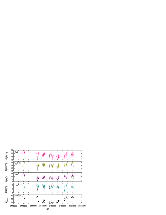
Figure 3.— Light curves of Fe ii , H$\beta^{n+b}$, H$\beta^{b}$ , H$\beta^{n}$ , $f_{\lambda}(5100\AA)$ (from top to bottom). Emission-line fluxes are displayed in units of $10^{-14}{\rm erg\ s}^{-1}\rm cm^{-2}$, the continuum flux determined from the power-law at 5100Å is given in units of $10^{-16}{\rm erg\ s}^{-1}\rm cm^{-2}$ Å^-1.

By IRAF-splot, the signal-to-noise ratios (S/Ns) between 7400Å and 7600Å in the observational frame are measured for these 39 spectra. Two spectra (2nd and 35th spectra: pg1700910712.fits, pg1700980414.fits) are ignored in our next analysis for their lower S/N less than 10 (Kaspi et al., 2000). For the left 37 spectra, the distribution of S/N is $25.3\pm 9$. The goodness of modeling of the Fe ii and continuum is tested by the elimination of Fe ii features at $\lambda 4924$ and $\lambda 5017$ (see Figure 2). We calculate the Fe ii flux by integrating the Fe ii template fit between $\lambda$4434 and $\lambda$4684. In Figure 3, we show the light curves of Fe ii , H$\beta^{n+b}$, H$\beta^{b}$ , H$\beta^{n}$ , and $f_{\lambda}(5100\AA)$ (from top to bottom).

We use the normalized variability measure defined by Kaspi et al. (2000) to compare the line variability to the continuum variability, $\sigma_{N}=100(\sigma^{2}-\delta^{2})^{1/2}/\bar{f}$, where $\bar{f}$ and $\sigma$ are the average and the rms of the flux in a given light curve, and $\delta$ is the mean uncertainty in a given light curve. The $\sigma_{N}$ are 6.73, 2.58, 8.46, 8.38, and 3.65 for the light curves of $f_{\lambda}(5100\AA)$ , Fe ii , H$\beta^{b}$ , H$\beta^{n}$ , and H$\beta^{n+b}$, respectively, in Figure 3. Kaspi et al. (2000) showed that $\sigma_{N}$ for the light curves of $f_{\lambda}(5100\AA)$ and H$\beta$ are 6.8, 3.2, with respectively, which are consistent with our results. And the $\sigma_{N}$ of Fe ii is smaller than that for $f_{\lambda}(5100\AA)$ , H$\beta^{b}$ , H$\beta^{n}$ , and H$\beta^{n+b}$.

3.2. Time lag from CCCD

Figure 4.— Cross-correlation functions (CCFs) for the continuum–Fe ii (top left), the continuum–H$\beta^{n+b}$ (top right), the continuum–H$\beta^{b}$(bottom left), and the continuum–H$\beta^{n}$ (bottom right) for PG 1700+518.

Figure 5.— Cross-correlation centroid distributions (CCCDs) for the continuum–Fe ii cross-correlation (top left), the continuum–H$\beta^{n+b}$ cross-correlation (top right), the continuum–H$\beta^{b}$ cross-correlation (bottom left), and the continuum–H$\beta^{n}$ cross-correlation (bottom right) for PG 1700+518.

The measurement of the line time lag, $\tau$, is made by cross-correlating the emission line and continuum light curves. In order to compare with the result of (Peterson et al., 2004), we use their code to do the line lag measurements. In Figure 4, we give the interpolated cross-correlation functions (CCF) for the continuum–Fe ii (top left), the continuum–H$\beta^{n+b}$ (top right), the continuum–H$\beta^{b}$(bottom left), and the continuum-H$\beta^{n}$ (bottom right) for PG 1700+518. We find a peak in the CCF for Fe ii light curve, which can be used to determine the time lag for Fe ii curve (Figures 4, 5). Because of many peaks with positive lag times and/or peaks with negative lag times in the CCFs for other three curves, we can’t determine their time lags (Figures 4 and 5).

Through the Monte Carlo FR/RSS method, the uncertainty of $\tau$ can be determined (Peterson et al. 2004). In the code, we adopt a minimum correlation coefficient of 0.4, the centroid threshold of 0.8 $R_{\rm max}$, and the number of trials is 3000 (Peterson et al. 2004). In Figure 5, we give the cross-correlation centroid distributions (CCCDs) for the continuum–Fe ii cross-correlation (top left) and the continuum–H$\beta^{n+b}$ cross-correlation (top right) for PG 1700+518, as well as that for H$\beta^{b}$ and H$\beta^{n}$ (bottom panels). It is obvious that the CCCD for Fe ii have a narrow positive peak. Following the suggestion given by (Peterson et al., 2004), we calculate the mean of the CCCD in all valid trials as the Fe ii centroid time lag, as well as its upper and lower uncertainties. We find that Fe ii time lag ,$\rm\tau_{\rm FeII}$, in PG 1700+518 is $270^{+130}_{-190}$ days. Its mean CCF $R_{\rm max}$ is $0.54\pm 0.08$. There are many positive peaks and/or strong negative peaks for H$\beta$ , H$\beta^{n}$ , and H$\beta^{b}$ . Therefore, we cannot give the line lags for H$\beta$ , H$\beta^{n}$ , and H$\beta^{b}$ . With the redshift of 0.292 for PG 1700+815, in the rest frame, the Fe ii time lag in PG1700+518 is $209^{+100}_{-147}$ days. Because the H$\beta$ time lag cannot be determined, we do not know whether the region emitting Fe ii is located outside of the region emitting the broad H$\beta$ lines (Marziani et al., 2003b; Vestergaard & Peterson, 2005; Popovic et al., 2007; Hu et al., 2008b; Kuehn et al., 2008).

4. Discussion

4.1. The Fe ii fitting method

In the analysis of the optical Fe ii light curve for PG 1700+518, we fit the optical spectrum by the Fe ii template instead of directly calculating the optical Fe ii flux in the selected wavelength range (e.g., Kuehn et al., 2008). In modeling Fe ii emission, we simultaneously model the power-law continuum, which is different from Wang et al. (2005) in the Fe ii analysis of an NLS1 NGC 4051. We also consider various FWHMs, centroid wavelength shifts and fluxes in the convolving of the Fe ii template. The accuracy of the measurement for the continuum shape depends on the wavelength coverage. For these 37 spectra of PG 1700+518, the wavelength coverage is mainly between $\sim$ 3500Åand $\sim$ 6000Å in the rest frame. Vestergaard & Peterson (2005) found that the optical Fe ii feature to the blue of H$\beta$ is contaminated by He i $\lambda 4471$ and He ii $\lambda 4686$ lines. For PG 1700+518, the He i $\lambda 4471$ and He ii $\lambda 4686$ lines are not strong (Figure 1). Therefore, we use the fitting windows of 4430-4770 and 5080-5550Å to exclude the emission lines of H$\beta$ , H$\gamma$ $\lambda 4340$, and [O iii] $\lambda\lambda$4959, 5007 (Figure 2). When we mask the region of He ii $\lambda 4686$ in the fitting, the fitting result is almost the same. We tried Fe ii template of Veron-Cetty et al. (2004), it is almost the same to that of I ZW 1.

4.2. The optical Fe ii emitting region

Kuehn et al. (2008) presented the reverberation analysis of optical Fe ii for Ark 120. They gave the light curves of the blue/red side of Fe ii , H$\beta$ , and continuum by setting the measurement windows (Figure 1 in Kuehn et al. 2008). Although the Fe ii cross-correlation function is very broad and flat-topped, they suggested that the optical Fe ii –emitting region, $\sim 320$ days, is several times larger than the H$\beta$ zone ($\sim 57$ days).Kuehn et al. (2008) found that it is difficult to constrain the FWHM of optical Fe ii for Ark 120 because of its very smooth Fe ii emission (Figure 8 in Kuehn et al. 2008). Modeling the Fe ii emission in PG 1700+518, we find that the mean value of Fe ii FWHM is $1554\pm 110$ km s^-1 . Because the change of H$\beta$ profile due to the Fe ii contribution is not too much (Figure 1), we adopted the H$\beta$ FWHM value of $1846\pm 682$ km s^-1 by Peterson et al. (2004). We find that $\rm(FWHM_{H\beta}/FWHM_{FeII})^{2}=1.41$. Assuming that Fe ii and H$\beta$ emission regions follow the virial relation between the time lag and the FWHM for the H$\beta$ and Fe ii emission lines, we can derive that the H$\beta$ time lag is $148^{+72}_{-104}$ days. We also find taht the new estimated H$\beta$ time lag is consistent with $R_{\rm BLR}-\lambda L_{\lambda}(5100\AA)$ relation by Bentz et al. (2009, see  their  Figure  5).

Considering the host contribution in $f_{\lambda}(5100\AA)$ , Bentz et al. (2009) suggested a new relation between BLRs size and $\lambda L_{\lambda}(5100\AA)$ , $\log R_{\rm BLR}=(-21.3^{+2.9}_{-2.8})+(0.519^{+0.063}_{-0.066})\log\lambda L_{\lambda}(5100\AA)~{}~{}\rm(lt-days)$. Kaspi et al. (2000) gave the average flux of $f_{\lambda}(5100\AA)$ (between 6520 and 6570 Å) without excluding Fe ii contribution, $(22.0\pm 1.5)\times 10^{-16}{\rm erg\ s}^{-1}\rm cm^{-2}$Å^-1. After excluding Fe ii contribution, we find that the value of $f_{\lambda}(5100\AA)$ at 5100Å is $(21.4\pm 1.5)\times 10^{-16}{\rm erg\ s}^{-1}\rm cm^{-2}$Å^-1. Therefore, the Fe ii correction is very small for $f_{\lambda}(5100\AA)$ . Corrected the contribution from starlight, Bentz et al. (2009) gave $f_{\lambda}(5100\AA)$ as $(18.5\pm 1.5)^{-16}{\rm erg\ s}^{-1}\rm cm^{-2}$Å^-1 and $\lambda L_{\lambda}(5100\AA)$ as $3.63\times 10^{45}{\rm erg\ s}^{-1}$ (the starlight contribution is about 16% in its total flux). The expected $R_{\rm BLR}$ from $R_{\rm BLR}-\lambda L_{\lambda}(5100\AA)$ relation (Bentz et al., 2009) and $\lambda L_{\lambda}(5100\AA)$ of $3.63\times 10^{45}{\rm erg\ s}^{-1}$ is 222 lt-days. Considering the larger uncertainty of intercept in this relation (about 3 in $\log R_{\rm BLR}$), this result is consistent with our estimated H$\beta$ time lag, $148^{+72}_{-104}$ days (Bentz et al., 2009, see  their  Figure  5).

If we take the FWHM/time lag uncertainties into consideration, the Fe ii emission region is located near the H$\beta$ emission region, not conclusively located outside of the H$\beta$ emission region. Kuehn et al. (2008) suggested that optical Fe ii emission is possibly produced at the dust sublimation radius, $R_{\rm dust}=476\times[L_{\rm bol}/10^{45}{\rm erg\ s}^{-1}]^{0.5}~{}~{}\rm(lt-days)$ (Elitzur & Shlosman, 2006). By $L_{\rm bol}=9\lambda L_{\lambda}(5100\AA)$, for PG1700+518, we find that the dust sublimation radius $R_{\rm dust}\sim 2868~{}~{}\rm(lt-days)$, which is much larger than the radius indicated by the Fe ii emission lag time.

Kaspi et al. (2000) measured the H$\beta$ flux between 6120Å and 6410 Å in the observational frame (also in Peterson et al. 2004). Their H$\beta$ fluxes include Fe ii contribution. Kaspi et al. (2000) gave H$\beta$ flux as $(18.88\pm 0.99)\times 10^{-14}{\rm erg\ s}^{-1}\rm cm^{-2}$. Removing Fe ii contamination in this region, the H$\beta$ flux is $(14.22\pm 1.01)\times 10^{-14}{\rm erg\ s}^{-1}\rm cm^{-2}$. With our new light curve for H$\beta$ , we cannot determine the time lag for H$\beta$ emission line, and we can determine the time lag for Fe ii line. It is possible due to: (1)H$\beta$ line has a asymmetric profile (Figure 2; narrow and broad components), suggesting that H$\beta$ is coming from the region with a very broad size and Fe ii is coming from the region with a narrow size. Therefore, we can detect Fe ii time lag. The H$\beta$ flux inKaspi et al. (2000) and Peterson et al. (2004) includes Fe ii contribution. (2)Peterson et al. (2004) found two peaks in its CCCD (see their Figure 15) and suggested that the peak at zero is due to correlated error. The spectral S/Ns are not high and the time sampling in the light curves is not good. More data and higher S/N spectra are needed in the future.

With respect to the H$\beta$ time lag of 252 days suggested by Peterson et al. (2004), smaller estimated H$\beta$ time lag of 148 days, which leads to the smaller black hole mass estimation in the logarithm, is decreased by 0.23 dex. However, considering the uncertainties of time lag and the mass calculation, our results are consistent with that from Peterson et al. (2004).

4.3. The relation between the spectral index and $f_{\lambda}(5100\AA)$ 

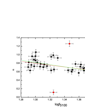
Figure 6.— Spectral slope, $\alpha$, vs. $f_{\lambda}(5100\AA)$ , $f_{\nu}\propto\nu^{-\alpha}$. Considering the error of $\alpha$, the red line is the best linear fit. The green line is the best linear fit excluding two discrete red points.

In our previous work Pu et al. (2006), we investigated the relation between the spectral index and $f_{\lambda}(5100\AA)$ and found almost all (15/17) PG QSOs showed an anti-correlation between them, except PG 1700+518 and PG 1229+204. For PG 1229+204, it is due to the system difference in two telescopes. For PG 1700+518, we suggested that it is maybe due to the Fe ii contribution (Pu et al., 2006). Here, we give this relation for PG 1700+518 when Fe ii contribution is carefully removed. We find that there is a strong anti-correlation between them (see Figure 6). The spearman coefficient $R$ is -0.33, with a probability of $p_{\rm null}<0.05$ for rejecting the null hypothesis of no correlation. If two discrete red points are excluded, $R$ is 0.55, and $p_{\rm null}<5.8\times 10^{-4}$. Therefore, after considering Fe ii contribution, PG 1700+518 shares the same characteristic on spectral slope variability as other 15 PG QSOs in our previous paper (Pu et al., 2006), i.e., harder spectrum during brighter phase (Hubeny et al. 2000).

5. Conclusion

With the spectral decomposition of 39 spectra of PG 1700+518 with the strong Fe ii emission, we investigate the Fe ii variability and its time lag. The main conclusions can be summarized as follows: (1) we give light curves of $f_{\lambda}(5100\AA)$ , Fe ii , H$\beta^{b}$ , H$\beta^{n}$ , and H$\beta$ ^n+b, as well as the mean and rms spectra for PG 1700+518. With the normalized variability measure, $\sigma_{N}$, we find that all components are variable. (2) With the code of Peterson et al. (2004), we find that Fe ii time lag in PG1700+518 is $209^{+100}_{-147}$ days, and H$\beta$ time lag cannot be determined. (3) Considering the uncertainties of time lags, the expected H$\beta$ time lag from the empirical luminosity–size relation is 221.6 lt-days, consistent with our measured Fe ii time lag. If we take FWHM/time lag uncertainties into consideration, Fe ii emission region is located near the H$\beta$ emission region, not conclusively located outside of the H$\beta$ emission region. (4) Assuming that Fe ii and H$\beta$ emission regions follow the virial relation between the time lag and the FWHM for the H$\beta$ and Fe ii emission lines, we can derive that the H$\beta$ time lag is $148^{+72}_{-104}$ days. With respect to the H$\beta$ time lag of 252 days suggested by Peterson et al. (2004), smaller H$\beta$ time lag, which leads to the black hole mass estimation in the logarithm, is decreased by 0.23 dex. (5) After considering Fe ii contribution, PG 1700+518 shares the same characteristic on spectral slope variability to other 15 PG QSOs in our previous work (Pu et al., 2006), i.e., harder spectrum during brighter phase.

References

- Baldwin et al. (2004) Baldwin, J. A., Ferland, G. J., Korista, K. T., Hamann, F., & LaCluyzé, A. 2004, ApJ, 615, 610
- Blandford et al. (1982) Blandford, R. D., & McKee, C. F. 1982, ApJ, 255, 419
- Bentz et al. (2009) Bentz, M. C., et al. 2009, ApJ, 697, 160
- Bian & Zhao (2004) Bian, W. H., & Zhao, Y. H. 2004, MNRAS, 347, 607
- Bian et al. (2008) Bian, W. H., et al., 2008, Chin. J. Astro. Astrophys, 8, 552
- Blandford & McKee (1982) Blandford, R. D., & McKee, C. F. 1982, ApJ, 255, 419
- Boroson & Green (1992) Boroson, T. A., & Green, R. F. 1992, ApJS, 80, 109
- Cardelli et al. (1989) Cardelli, J. A., Clayton, G. C., & Mathis, J. S., 1989, ApJ, 345, 245
- Elitzur & Shlosman (2006) Elitzur, M., & Shlosman, I., 2006, ApJ, 648, L101
- Greene & Ho (2005) Greene, J. E., & Ho, L. C. 2005,ApJ, 630, 122
- Hu et al. (2008b) Hu C., Wang J. M., Ho L. C., Chen Y. M., Bian W. H., & Xue S. J., 2008b, ApJL, 683, L115
- Hu et al. (2008a) Hu C., Wang J. M., Ho L. C., Chen Y. M., Zhang H. T., Bian W. H., & Xue S. J., 2008a, ApJ, 687, 78
- Hubeny et al. (2000) Hubeny I., et al., 2000, ApJ, 533, 710
- Kaspi et al. (2005) Kaspi, S., Maoz, D., Netzer, H., Peterson, B.M., Vestergaard M., & Jannuzi B.T., 2005, ApJ, 629, 61
- Kaspi et al. (2000) Kaspi, S., Smith, P.S., Netzer, H., Maoz, D., ,Jannuzi, B.T., & Giveon U., 2000, ApJ, 533, 631
- Kuehn et al. (2008) Kuehn C. A., et al., 2008, ApJ, 673, 69
- Laor et al. (1997) Laor, A., Jannuzi, B. T., Green, R. F., & Boroson, T. A. 1997, ApJ, 489, 656
- Maoz et al. (1993) Maoz, D., et al., 1993, ApJ, 404, 576
- Marziani et al. (2003b) Marziani, P., Sulentic, J. W., Zamanov, R., Calvani, M., Dultzin-Hacyan, D., Bachev, R., & Zwitter, T. 2003b, ApJS, 145, 199
- Marziani et al. (2003a) Marziani, P., Zamanov, R. K., Sulentic, J. W., & Calvani, M. 2003a, MNRAS, 345, 1133
- McLure & Jarvis (2004) McLure, R. J., & Jarvis, M. J. 2004, MNRAS, 353, L45
- O’Donnell (1994) O’Donnell, J. E. 1994, ApJ, 422, 158
- Peterson (1993) Peterson, B. M. 1993, PASP, 105, 247
- Peterson et al. (2004) Peterson, B. M., et al., ApJ, 2004, 613, 682
- Popovic et al. (2007) Popović, L. Č., Smirnova, A., Ilić, D., Moiseev, A., Kovačević, J., & Afanasiev, V. 2007, in ASP Conf. Ser. 373, The Central Engine of Active Galactic Nuclei, ed. L. C. Ho & J.-M. Wang (San Francisco, CA: ASP), 552
- Pu et al. (2006) Pu, X. T, Bian, W. H., & Huang, K. L., 2006, MNRAS, 372, 246
- Turnshek et al. (1985) Turnshek, D. A., et al., 1985, ApJ, 294, L1
- Veron-Cetty et al. (2004) Véron-Cetty, M. P., Joly, M., & Véron, P., A&A, 2004, 4 17, 515
- Vestergaard & Peterson (2005) Vestergaard, M., & Peterson, B. M., 2005, ApJ, 625, 688
- Vestergaard & Wilkes (2001) Vestergaard, M., & Wilkes, B. J. 2001, ApJS, 134, 1
- Wang et al. (2005) Wang, J., Wei, J. Y., & He, X. T., 2005, A&A, 436, 417
- Wills et al. (1985) Wills, B. J., Netzer, H., & Wills, D. 1985, ApJ, 288, 94