Finite-size scaling theory for explosive percolation transitions

Abstract

The finite-size scaling (FSS) theory for continuous phase transitions has been useful in determining the critical behavior from the size dependent behaviors of thermodynamic quantities. When the phase transition is discontinuous, however, FSS approach has not been well established yet. Here, we develop a FSS theory for the explosive percolation transition arising in the Erdős and Rényi model under the Achlioptas process. A scaling function is derived based on the observed fact that the derivative of the curve of the order parameter at the critical point $t_{c}$ diverges with system size in a power-law manner, which is different from the conventional one based on the divergence of the correlation length at $t_{c}$. We show that the susceptibility is also described in the same scaling form. Numerical simulation data for different system sizes are well collapsed on the respective scaling functions.

Explosive percolation transition (PT) occurring in a modified Erdős and Rényi (ER) model has attracted considerable attention in physics communities in a short period science ; ziff ; cho ; santo ; herrmann1 ; souza ; herrmann2 ; friedman , because most studies of discontinuous phase transitions have been limited to equilibrium thermal systems. The modified ER model includes an additional rule that discourages the formation of a giant cluster, called the Achlioptas process (AP) science to the rule in the classic ER network model er . According to this rule, while a giant cluster develops slowly, many large-size clusters accumulate with their numbers exceeding to those in the critical state. After an enforced delay, a giant cluster is formed at a transition point by the aggregation of the large-size clusters, which proceeds in an extremely short time. Thus, the order parameter increases suddenly. In analogy to the eruption of a volcano or a seismic outbreak, this transition is called the explosive PT.

Finite-size scaling (FSS) theory has been useful for characterizing phase transitions. When the phase transition is continuous, the critical behavior of a system in the thermodynamic limit can be extracted from the size dependent behaviors of thermodynamic quantities. For example, the magnetization of ferromagnetic systems is assumed to follow a scaling form near the critical temperature $T_{c}$,

$$m=L^{-\beta/\nu}f((T-T_{c})L^{1/\nu}),$$ (1)

where $L$ is the lattice size, $f(x)$ is a scaling function, and $T$ is temperature. $\beta$ and $\nu$ are the critical exponents associated with the magnetization and the correlation length, respectively. This scaling function was set up based on the fact that the correlation length, which diverges as $T\to T_{c}$, is limited to the lattice size $L$. When the phase transition is discontinuous, however, the correlation length does not diverge. Thus, a new approach was needed. As a successful example, a scaling function was derived by using the probability distribution for the internal energy for the $q$-state Potts model with $q>4$ in two dimensions challa ; binder . However, FSS approach for discontinuous transitions arising in disordered systems has not been studied yet. In this Letter, we develop FSS theory for the discontinuous PT in the modified ER model under the AP, and obtain a scaling function, which has a different form from the conventional one (1).

In the classic ER model, a system is composed of a fixed number of vertices $N$, which evolves as one edge is randomly added to it at each time step. Hereafter, time is defined as the number of edges added to each node. In the ER model under the AP, at each time step, two edges are randomly selected, but only one of them is actually added to the system to minimize the product of the sizes of the clusters that are connected by the potential edge. The ER model based on this product rule is hereafter called the ERPR model. While the rule in the ERPR model may be too artificial to fit real systems, the ERPR model contains an intrinsic mechanism triggering discontinuous phase transitions. Thus, it is meaningful to develop a FSS theory with this ERPR model.

The size of the giant cluster is determined as $G_{N}(t)\equiv 1-\sum_{s}^{\prime}sn_{s}(t)$, where $n_{s}(t)$ is the density of $s$-size clusters at time $t$, and the largest cluster is excluded in the sum, denoted by the prime in the summation. Fig.1 shows $G_{N}(t)$ versus $t$ for different system sizes for the ERPR model. The curves of $G_{N}(t)$ for different $N$s intersect at approximately one point, namely, $t_{\rm x}\approx 0.88845(2)$. We consider the $t$-intercept of the tangent of the curve $G_{N}(t)$ at $t_{\rm x}$, denoted as $t_{d}(N)$. Then this time is calculated as

$$t_{d}(N)=t_{\rm x}-G_{N}(t_{\rm x})\Big{(}\frac{dG_{N}(t)}{dt}\Big{|}_{t=t_{\rm x}}\Big{)}^{-1}.$$ (2)

We find that as $N\to\infty$, the derivative of $G_{N}(t)$ at $t_{\rm x}$ diverges as

$$\frac{dG_{N}(t)}{dt}\Big{|}_{t=t_{\rm x}}\sim N^{\theta},$$ (3)

with $\theta\approx 0.48(1)$. Thus, the derivative diverges in the limit $N\to\infty$, indicating that the PT is indeed discontinuous.

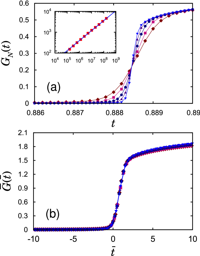
Figure 1: (Color online) (a) Plot of the giant cluster size per node $G_{N}(t)$ versus time $t$ for system sizes $N/10^{4}=128,$ 256, 512, 1024 and 2048. The curves intersect at $t_{\rm x}$, which is regarded as the transition point in the thermodynamic limit. Inset: Plot of $dG_{N}(t)/dt$ at $t_{\rm x}$ versus $N$. The solid line is a reference line with a slope of $0.48$. (b) The same plot with scaled variables ${\bar{G}}({\bar{t}})\equiv r^{-1}G({\bar{t}})$ and ${\bar{t}}\equiv(t-t_{d})r^{-1}\frac{dG_{N}}{dt}|_{t_{\rm x}}$, where $r=M_{2}^{2}(t_{d})/M_{3}(t_{d})$. Data for different system sizes are well collapsed in a single curve.

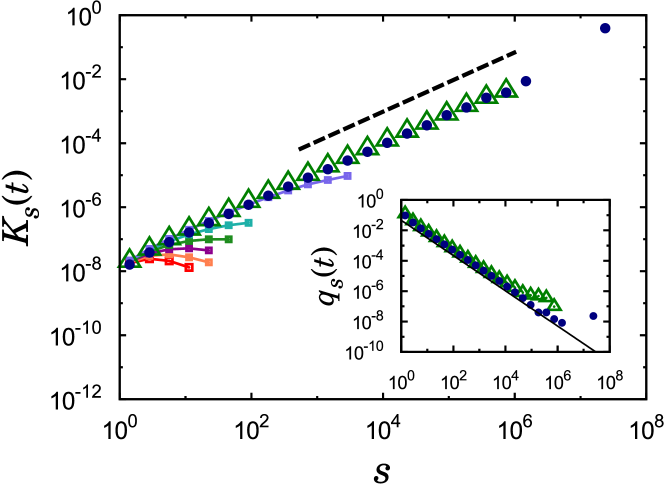
Figure 2: (Color online) Plot of $K_{s}(t)$ versus $s$ at various times for the ERPR network with system size $N=8.192\times 10^{7}$. The dashed line is a reference line with a slope of 0.92. The data correspond to $t=0.4$, 0.5, 0.6, 0.7, 0.8, 0.88, $t_{d}(\triangle)$, and $t_{z}(\circ)$ (starting from the bottom). Inset: Plot of $q_{s}(t_{d})(\triangle)$ and $q_{s}(t_{z})(\circ)$ versus $s$. The solid line is a reference line with a slope of $-1.16$.

Since the dynamics of the ERPR model involves the selection of two edges at each time step, it may be difficult to analytically clarify the evolution of the giant cluster. Thus, a simple model, called the cluster-aggregation network model, which involves the selection of one edge at each time step, was introduced can . This cluster-aggregation network model is a simple representation of the ERPR model, because the frequency of intercluster connections is dominant until the percolation threshold. In this model, once two clusters of sizes $i$ and $j$ are selected with probabilities $i^{\omega}/c(t)$ and $j^{\omega}/c(t)$, respectively, where $c(t)\equiv\sum_{s}s^{\omega}n_{s}(t)$, one vertex is chosen randomly from each selected cluster, and the two vertices are connected. When $\omega=1$, this model reduces to the ER network. To put the ERPR model in this perspective, we measure corresponding value of $\omega$ by measuring the probability $q_{s}(t)$ of an added edge being connected to a vertex in a cluster of size $s$ at time $t$. This probability is given by $q_{s}(t)=s^{\omega}n_{s}(t)/c(t)$ for the cluster-aggregation network model. Thus, by measuring $q_{s}(t)$ and $n_{s}(t)$, we calculate $s^{\omega}/c(t)$ for the ERPR model, which is denoted as $K_{s}(t)$. When $t\ll t_{d}(N)$, $K_{s}(t)$ does not exhibit a power-law behavior, however, as $t\to t_{d}(N)$, it does as $K_{s}(t)\sim s^{\omega}$ with $\omega\approx 0.92$ (Fig. 2). This power-law behavior persists as time progresses beyond $t_{d}(N)$.

Since $\omega_{\rm ERPR}\approx 0.92$ is close to $\omega_{\rm ER}=1$, we may get a hint on the evolution of the ERPR model in the context of the analytic formulae of the ER model. The explicit formula for the evolution of the giant component of the ER model with an arbitrary initial condition was calculated ziff2 ; can . For example, the giant cluster size near the transition point $t_{c}=\frac{1}{2M_{2}(0)}$ is

$$G^{\rm ER}(t)=\frac{2M_{2}^{2}(0)}{M_{3}(0)}\left(\frac{t}{t_{c}}-1\right),$$ (4)

where $M_{n}(0)=\sum_{s}^{\prime}s^{n}n_{s}(0)$ is the initial $n$-th moment. Thus, when a system starts an evolution from $n_{s}(0)=\delta_{s,1}$, thus $M_{2}(0)=M_{3}(0)=1$, the giant cluster size begins to grow from zero to a macroscopic scale continuously at the transition point $t_{c}=1/2$.

Here, we consider a particular initial condition, in which $M_{2}(0)$ and $M_{3}(0)$ depend on $N$. We assume that $n_{s}(0)$ follows a flat distribution, $n_{s}(0)=n_{0}$, in the range $0<s<s_{m}$, where $s_{m}$, the size of the largest cluster at $t=0$, depends on $N$ as $s_{m}=N^{\eta}$. Then, $n_{0}=2N^{-2\eta}$, $M_{2}(0)\propto N^{\eta}$, and $M_{3}(0)\propto N^{2\eta}$. Then, a PT takes place at $t_{c}(N)=1/2M_{2}(0)\propto N^{-\eta}$, and $G(t)\sim r(2M_{2}(0)t-1)$ for $t>t_{c}(N)$ from Eq. (4), where $r\equiv 2M_{2}^{2}(0)/M_{3}(0)$ turns out to be in $\mathcal{O}(1)$. Thus, if time $t$ is scaled as $t^{\prime}=tM_{2}(0)$, then $G(t^{\prime})$ has a mean field behavior similar to the original ER case. This scaling behavior implies that $t$ increases $\sim\mathcal{O}(N^{-\eta})$ beyond $t_{c}$, $G_{N}(t)$ does so by $\mathcal{O}(1)$. Thus, a discontinuous phase transition occurs. Generally, if the conditions that (i) the amplitude $M_{2}^{2}(0)/M_{3}(0)$ is finite and (ii) $M_{2}(0)$ diverges as $N\to\infty$ are fulfilled, a discontinuous PT can occur in the ER model. We show below that the origin of the explosive PT in the ERPR model can be understood in this scheme.

For further discussion, we reconsider the ER model with an initial condition $n_{s}(0)=\delta_{s,1}$. As time passes, small-size clusters develop, and thus the cluster-size distribution is no longer monodisperse. We take a certain time $t^{*}<t_{c}$ and the amplitude at that time is $r(t^{*})=2M_{2}^{2}(t^{*})/M_{3}(t^{*})$. Since the evolution of the ER model proceeds continuously, it holds that $G^{\rm ER}(t)=r(t^{*})[2M_{2}(t^{*})(t-t^{*})-1]$, in which the certain time $t^{*}$ is regarded as an ad hoc time origin. This relation has been checked numerically. We apply this logic to the evolution of the ERPR model below.

We examine the amplitude $M_{2}^{2}(t)/M_{3}(t)$ as a function of time for the ERPR model near the transition point, and find that it is finite but suddenly drops to zero in the thermodynamic limit (Fig. 3(a)). In the conventional ER model, however, $M_{2}^{2}(t)/M_{3}(t)$ is zero near the transition point, and thus, the transition is continuous (Fig. 3(a)). Interestingly, the time $t_{d}(N)$ defined in Eq.(3) locates approximately on the verge of the sudden drop in the amplitude (Fig. 3(b)). Thereby, we call $t_{d}(N)$ as the triggering time of the explosive PT. We examine the behavior of the amplitude and the second moment at $t_{d}(N)$ as a function of system size $N$ more carefully. We find the amplitude can be fit to a power law $M_{2}^{2}(t_{d})/M_{3}(t_{d})\sim N^{-\kappa}$. However, we find that $\kappa$ is very small and decrease slowly from $0.06$ to $0.04$, measured by successive slopes, as the system size increases from $10^{5}$ to $2\times 10^{7}$. Thus, one may regard $\kappa$ as zero. This suggests that the amplitude is independent of $N$ in the thermodynamic limit. However, $M_{2}(t_{d}(N))\sim N^{0.7}$. Next, we take $t_{d}(N)$ as the ad hoc time origin, and then $t_{d}(N)$ plays a role of the percolation threshold as we have seen that $t_{c}(N)\to 0$ as $N\to\infty$ in the ER model with the flat distribution. Indeed, $t_{d}(N)$ approaches $t_{\rm x}$ as in (2). From these results, we can conclude that the ERPR model satisfies the condition for a discontinuous phase transition at the ad hoc time origin. On the other hand, it was noticed friedman that the key ingredient to explosive transition was not the details of the dynamics during the actual explosion, but rather lay in the period preceding the explosion when a type of power keg developed. This ingredient is embodied in the moments of the cluster size distribution at $t_{d}(N)$, which satisfies the conditions (i) and (ii). Thus, the explosive PT takes place.

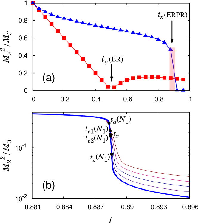
Figure 3: (Color online) (a) Plot of the amplitude $M_{2}^{2}(t)/M_{3}(t)$ versus time $t$ for the ERPR network ($\triangle$, blue) with system size $N_{1}=2.048\times 10^{7}$ and for the ER model ($\square$, red). (b) Zoom-in plot of the amplitude versus $t$ for the ERPR network with different system sizes $N=1.28\times 10^{6}$, $2.56\times 10^{6}$, $5.12\times 10^{6}$ $1.024\times 10^{7}$ and $2.048\times 10^{7}$ from the top. The amplitude decreases more drastically as system size is increased. Various characteristic times are indicated on the curve for $N=N_{1}$. The explosion starts at $t_{d}(N)$ and ends at $t_{z}(N)$. The two kinds of susceptibility reach their maximum at $t_{c1}$ and $t_{c2}$, respectively, while the crossing time $t_{x}$ is independent of $N$.

We derive a scaling function for the ERPR model, inspired by the formula (4). Since $\omega^{\rm ERPR}\neq\omega^{\rm ER}$, we take a general form of the giant cluster size, $G(t)=r(ut-1)$, where $r$ and $u$ can depend on $N$ and $t$. Since we take $t_{d}(N)$ as the ad hoc time origin, we calculate $r$ and $u$ at $t_{d}(N)$, and substitute $t\to t-t_{d}(N)$. Then, we obtain that $u(t_{d})=r^{-1}(t_{d})\frac{dG_{N}}{dt}|_{t_{\rm x}}$, which is not $M_{2}(t_{d})$ as in the ER case. We assume that $r(t_{d})$ follows the same form $M_{2}^{2}(t_{d})/M_{3}(t_{d})$ from the ER model. Thus, our FSS form becomes $G_{N}(t)=r(t_{d})\bar{G}(\bar{t})$, where $\bar{G}(x)$ is a scaling function and $\bar{t}\equiv(t-t_{d})r^{-1}\frac{dG_{N}}{dt}|_{t_{x}}$. Then,

$$G_{N}(t)=N^{-\beta/{\bar{\nu}}}f_{0}\big{(}(t-t_{d}(N))N^{1/{\bar{\nu}}}\big{)},$$ (5)

where $f_{0}(x)$ is a scaling function and $\beta/{\bar{\nu}}=\kappa$ and $1/{\bar{\nu}}=\theta+\kappa$. We confirm this scaling function with numerical data obtained for different system sizes as shown in Fig. 1(b). Even though we obtain $\kappa\approx 0.06-0.04$ in our simulation range of system size, we expect $\beta/{\bar{\nu}}=0$ asymptotically and thus $1/{\bar{\nu}}\approx 0.48(1)$ and $\beta=0$. We notice that the scaling function is in a particular form: Instead of following the conventional form $t-t_{\rm x}$ in its argument, the scaling function in (5) contains the form $t-t_{d}(N)$, implying that the interval $t-t_{d}(N)$ can change with $N$ for a fixed $t$.

We define the susceptibility in two ways. The first is the mean cluster size $\chi_{1}(t)\equiv\sum_{s}^{\prime}s^{2}n_{s}(t)/\sum_{s}^{\prime}sn_{s}(t)$, which exhibits a peak at $t_{c1}(N)$. $t_{c1}(N)$ is larger than both $t_{d}(N)$ and $t_{\rm x}$, but approaches $t_{x}^{+}$ as $N\to\infty$. The susceptibility at $t_{c1}(N)$ increases with $N$ as $\chi_{1}(t_{c1}(N))\sim N^{0.7}$, confirming the previous result santo2 , which also behaves in the same manner at $t_{d}(N)$. Thus, $\chi_{1}(t)$ is written in the form $\chi_{1}(t)=N^{\gamma_{1}/{\bar{\nu}}}f_{1}\big{(}(t-t_{d})N^{1/{\bar{\nu}}}\big{)}$, where $f_{1}(x)$ is another scaling function. Thus, $\gamma_{1}/{\bar{\nu}}\approx 0.7$. The second one is the fluctuation of the giant component sizes defined as $\chi_{2}(t)\equiv N\sqrt{\langle G_{N}^{2}(t)\rangle-\langle G_{N}(t)\rangle^{2}}$. This quantity exhibits a peak at $t_{c2}$. We find that $\chi_{2}(t_{c2}(N))\sim N$, which holds even at $t_{d}(N)$. Thus, $\gamma_{2}/{\bar{\nu}}=1$ and $\chi_{2}(t)=Nf_{2}\big{(}(t-t_{d})N^{1/{\bar{\nu}}}\big{)}$ with a scaling function $f_{2}$. The scaling behaviors are confirmed numerically in Fig. 4.

To catch the physical meaning of $t_{d}(N)$ further, we investigate the cluster size distribution $n_{s}(t)$ as a function of time $t$. In early times, $n_{s}(t)$ decays exponentially. As time passes, it exhibits a power-law behavior in small cluster-size region, but a hump develops in the tail region. We represent $n_{s}(t)$ as $n_{s}(t)\sim s^{-\tau(t)}g(s,t,N)$, where the exponent $\tau(t)$ is weakly dependent on time $t$ and ranges from $\tau\approx 2.05(2)-2.09(1)$ as time progresses beyond $t_{d}(N)$. $g(s,t,N)$ represents the shape of the hump. To estimate the hump size, we first plot $n_{s}(t)s^{\tau}$ versus $s$ for different times and define the hump size as the number of nodes in the shade region in Fig.5. As time passes, the shape area increases and attains a maximum at $t_{m}(N)$, and then it reduces to zero at time $t_{z}(N)$. In fact, $t_{z}(N)$ is defined as the point at which the size distribution of finite clusters follows a power law. We obtain the value of $\tau$ at $t_{z}$ as $\tau\approx 2.09(1)$ self . The characteristic time $t_{m}(N)$ is numerically consistent with $t_{d}(N)$, indicating that indeed $t_{d}(N)$ is the triggering time of the explosive PT, and the powder keg becomes empty at $t_{z}(N)$.

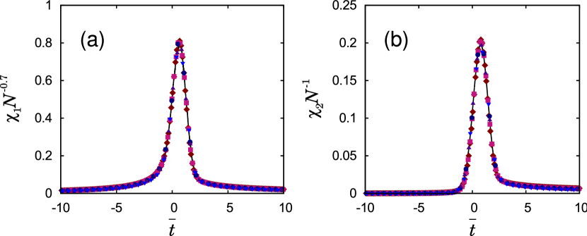
Figure 4: (Color online) (a) Plot of the susceptibility $\chi_{1}$, the mean cluster size, versus time in a scaled form for different system sizes used in Fig. 1. ${\bar{t}}\equiv(t-t_{d})r^{-1}\frac{dG_{N}}{dt}|_{t_{\rm x}}$, where $r\equiv M_{2}^{2}(t_{d})/M_{3}(t_{d})$. (b) Similar plot for the susceptibility $\chi_{2}$, the fluctuation of the giant cluster size, versus time in a scaled form.

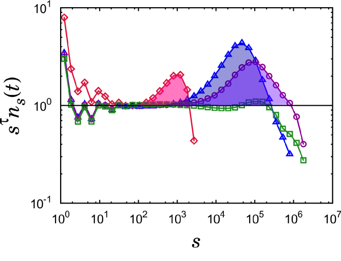
Figure 5: (Color online) Plot of $s^{\tau}n_{s}(t)$ versus $s$ for different times $t=0.884(\diamond)$, $t_{d}(\triangle)$, $t_{c1}(\circ)$ and $t_{z}(\square)$ for the ERPR model with size $N=1.024\times 10^{7}$. The hump size, the number of nodes contained in the shade area, becomes maximum at time $t_{d}(N)$, beyond which it reduces.

In summary, we have found that the curves of the giant component size $G_{N}(t)$ for different system sizes $N$s intersect at the transition point $t_{\rm x}$, and the derivative of $G_{N}(t)$ with respect to $t$ at $t_{\rm x}$ diverges in a power-law manner as $N$ increases. This indicates that the explosive PT is manifestly discontinuous. We also found that the evolution can be regarded as kinetic cluster aggregations in which the connection kernel turns out to be similar to that for the conventional ER model near the transition point. Based on these facts, we have developed a finite-size scaling theory for for the behavior of the explosive PT, which has a different origin from the conventional one for continuous phase transitions, and thus has a different form. We have determined the critical exponents. The method we develop here can also be used for other percolating systems exhibiting discontinuous transitions, for example, in the interacting complex networks havlin .

This study was supported by an NRF grant awarded through the Acceleration Research Program (Grant No. 2010-0015066) (BK), the NAP of KRCF (DK) and the Seoul Science Foundation (YSC).

References

- (1) D. Achlioptas, R. M. D’Souza, and J. Spencer, Science 323, 1453 (2009).
- (2) R. M. Ziff, Phys. Rev. Lett. 103, 045701 (2009).
- (3) Y.S. Cho, J.S. Kim, J. Park, B. Kahng, and D. Kim, Phys. Rev. Lett. 103, 135702 (2009).
- (4) F. Radicchi and S. Fortunato, Phys. Rev. Lett. 103, 168701 (2009).
- (5) A.A Moreira, E.A. Oliveira, S.D.S. Reis, H.J. Herrmann, J.S. Andrade Jr., Phys. Rev. E 81, 040101 (2010).
- (6) R.M. D’Souza and M. Mitzenmacher, Phys. Rev. Lett. 104, 195702 (2010).
- (7) N. A. M. Arújo and H. J. Herrmann, arXiv:1005.2504.
- (8) E.J. Friedman and A.S. Landsberg, Phys. Rev. Lett. 103, 255701 (2009).
- (9) P. Erdős, A. Rényi, Publ. Math. Hugar. Acad. Sci. 5, 17 (1960).
- (10) M.S.S. Challa, D.P. Landau and K. Binder, Phys. Rev. B 34, 1841 (1986).
- (11) K. Binder, Rep. Prog. Phys. 50, 783 (1987).
- (12) Y.S. Cho, B. Kahng and D. Kim, Phys. Rev. E. 81, 030103(R) (2010).
- (13) R.M. Ziff, E.M. Hendriks, and M.H. Ernst, Phys. Rev. Lett. 49, 593 (1982).
- (14) F. Radicchi and S. Fortunato, Phys. Rev. E 81, 036110 (2010).
- (15) The measured value is related to by the relationship but with logarithmic correction, which can be shown analytically.
- (16) S.V. Buldyrev, R. Parshani, G. Paul, H.E. Stanley, and S. Havlin, Nature 464, 1025 (2010).