Subspace Evolution and Transfer (SET) for Low-Rank Matrix Completion

Abstract

We describe a new algorithm, termed subspace evolution and transfer (SET), for solving low-rank matrix completion problems. The algorithm takes as its input a subset of entries of a low-rank matrix, and outputs one low-rank matrix consistent with the given observations. The completion task is accomplished by searching for a column space on the Grassmann manifold that matches the incomplete observations. The SET algorithm consists of two parts – subspace evolution and subspace transfer. In the evolution part, we use a gradient descent method on the Grassmann manifold to refine our estimate of the column space. Since the gradient descent algorithm is not guaranteed to converge, due to the existence of barriers along the search path, we design a new mechanism for detecting barriers and transferring the estimated column space across the barriers. This mechanism constitutes the core of the transfer step of the algorithm. The SET algorithm exhibits excellent empirical performance for both high and low sampling rate regimes.

I Introduction

Suppose that we observe a subset of entries of a matrix. The matrix completion problem asks when and how the matrix can be recovered based on the observed entries. In general, this reconstruction task is ill-posed and computationally intractable. However, if the data matrix is known to have low-rank, exact recovery can be accomplished in an efficient manner with high probability, provided that sufficiently many entries are revealed. Low-rank matrix completion problems have received considerable interests due to their wide applications, ranging from collaborative filtering (the NETFLIX challenge) to sensor network tomography. For an overview of these applications, the reader is referred to [1].

An efficient way to solve the completion problem is via convex relaxation. Instead of looking at rank-restricted matrices, one can search for a matrix with minimum nuclear norm, subject to data consistency constraints. Although in general nuclear norm minimization is not equivalent to rank minimization, the former approach recovers the same solution as the latter if the data matrix satisfies certain incoherence conditions [2]. More importantly, nuclear norm minimization can be accomplished in polynomial time by using semi-definite programming, singular value thresholding (SVT) [3], or methods adapted from robust principal component analysis [4].

Several low-complexity alternatives to nuclear norm minimization have been proposed so far. Realizing the intimate relationship between compressive sensing and low-rank matrix completion, a few approaches for low-rank completion can be viewed as generalization of those for compressive sensing reconstruction. In particular, the ADMiRA algorithm [5] is a counterpart of the subspace pursuit (SP) [6] and CoSaMP [7] algorithms, while the singular value projection (SVP) method [8] extends the iterative hard thresholding (IHT) [9] approach. There are other approaches that rely more on the specific structures of the low-rank matrices. The power factorization algorithm described in [10] takes an alternating optimization approach. In the OptSpace algorithm described in [11], a simultaneous optimization on both column and row spaces is employed.

We address a more general class of problems in low-rank matrix completion – consistent completion. Consistent completion extends the previous completion framework in that it does not require the existence of a unique solution to the problem. This extension seems questionable at first glance – in highly undersampled observation regimes, there may exist many low-rank matrices that match the observations – which makes the final result have less practical value. Nevertheless, the consistent completion paradigm allows for identifying convergence problems with standard completion techniques, and it does not require any additional structure on the matrix, such as incoherence. Furthermore, as will be shown in the subsequent exposition, when confronted with very sparsely sampled matrices all methods known so far fail to produce any solution to the problem, despite the fact that many exist. Finally, even in the sampling regime for which SVT, OptSpace and other techniques have provable, unique reconstruction performance guarantees, the consistent completion technique described in this contribution exhibits significantly better results.

To solve the consistent matrix completion problem, we propose a novel subspace evolution and transfer (SET) method. We show that the matrix completion problem can be solved by searching for a column space (or, alternatively, for a row space) that matches the observations. As a result, optimization on the Grassmann manifold, i.e., subspace evolution, plays a central role in the algorithm. However, there may exist “barriers” along the search path that prevent subspace evolution from converging to a global optimum. To address this problem, in the subspace transfer part, we design mechanisms to detect and cross barriers. The SET algorithm improves the recovery performance not only in high sampling rate regime but also in low sampling rate regime where there may exist many low-rank solutions. Empirical simulations demonstrate the excellent performance of the proposed algorithm.

The SET algorithm employs a similar approach as that of the OptSpace algorithm [11] in terms of using optimization over Grassmann manifolds. Still, the SET approach substantially differs from the method supporting OptSpace [11]. Searching over only one space (column or row space) represents one of the most significant differences: in OptSpace, one searches both column and row spaces simultaneously, which introduces numerical and analytical difficulties. Moreover, when optimizing over the column space, one has to take care of “barriers” that prevent the search procedure from converging to a global optimum, an issue that was not addressed before since it was obscured by simultaneous column and row space searches.

The paper is organized as follows. In Section II we introduce the consistent low-rank completion problem, and describe the terminology used throughout the paper. In Section III we outline the steps of the SET algorithm. Simulation results are presented in Section IV. All proofs are listed in the Appendix sections.

II Consistent Matrix Completion

Let $\bm{X}\in\mathbb{R}^{m\times n}$ be an unknown matrix with rank $r\ll\min\left(m,n\right)$, and let $\Omega\subset\left[m\right]\times\left[n\right]$ be the set of indices of the observed entries, where $\left[K\right]=\left\{1,2,\cdots,K\right\}$. Define the projection operator $\mathcal{P}_{\Omega}$ by

$$\mathcal{P}_{\Omega}:\;\mathbb{R}^{m\times n} \rightarrow\mathbb{R}^{m\times n}$$

$$\mathcal{P}_{\Omega}(\bm{X}) \mapsto\bm{X}_{\Omega},\;\mbox{where }\left(\bm{X}_{\Omega}\right)_{i,j}=\begin{cases}\bm{X}_{i,j}&\mbox{if }\left(i,j\right)\in\Omega\\ 0&\mbox{if }\left(i,j\right)\notin\Omega\end{cases}.$$

The consistent matrix completion problem is to find one rank-$r$ matrix $\bm{X}^{\prime}$ that is consistent with the observations $\bm{X}_{\Omega}$, i.e.,

$$\left(P0\right):\; \mbox{find a }\bm{X}^{\prime}\mbox{ such that }$$

$$\mbox{rank}\left(\bm{X}^{\prime}\right)\leq r\mbox{ and }\mathcal{P}_{\Omega}\left(\bm{X}^{\prime}\right)=\mathcal{P}_{\Omega}\left(\bm{X}\right)=\bm{X}_{\Omega}.$$ (1)

This problem is well defined as all our instances of $\bm{X}_{\Omega}$ are generated from matrices $\bm{X}$ with rank $r$ and therefore there must exist at least one solution. Here, like in other approaches [5, 10, 11], we assume that the rank $r$ is given. In practice, one may try to sequentially guess a rank bound until a satisfactory solution has been found.

We also introduce the (standard) projection operator $\mathcal{P}$,

$$\mathcal{P}:\;\mathbb{R}^{m}\times\mathbb{R}^{m\times k} \rightarrow\mathbb{R}^{m}$$

$$\mathcal{P}\left(\bm{x},\bm{U}\right) \mapsto\bm{y}=\bm{U}\bm{U}^{\dagger}\bm{x},$$

where $1\leq k\leq m$, and where the superscript $\dagger$ denotes the pseudoinverse of a matrix. That is, $\mathcal{P}\left(\bm{x},\bm{U}\right)$ gives the projection of the vector $\bm{x}$ on the hyperplane spanned by the matrix $\bm{U}$, i.e., $\mbox{span}\left(\bm{U}\right)$. It should be observed that $\bm{U}^{\dagger}\bm{x}$ is the global minimizer of the quadratic optimization problem $\min_{\bm{w}\in\mathbb{R}^{k}}\;\left\|\bm{x}-\bm{U}\bm{w}\right\|_{F}^{2}.$

II-A Why optimizing over column spaces only?

In this section, we show that the problem $\left(P0\right)$ is equivalent to finding a column space consistent with the observations.

Let $\mathcal{U}_{m,r}$ be the set of $m\times r$ matrices with $r$ orthonormal columns, i.e., $\mathcal{U}_{m,r}=\left\{\bm{U}\in\mathbb{R}^{m\times r}:\;\bm{U}^{T}\bm{U}=\bm{I}_{r}\right\}.$ Define a function

$$f:\;\mathcal{U}_{m,r} \rightarrow\mathbb{R}$$

$$f(\bm{U}) \mapsto\underset{\bm{W}\in\mathbb{R}^{n\times r}}{\min}\left\|\bm{X}_{\Omega}-\mathcal{P}_{\Omega}\left(\bm{U}\bm{W}^{T}\right)\right\|_{F}^{2},$$ (2)

where $\left\|\cdot\right\|_{F}$ denotes the Frobenius norm. The function $f$ captures the consistency between the matrix $\bm{U}$ and the observations $\bm{X}_{\Omega}$ : if $f\left(\bm{U}\right)=0$, then there exists a matrix $\bm{W}$ such that the rank-$r$ matrix $\bm{U}\bm{W}^{T}$ satisfies $\mathcal{P}_{\Omega}\left(\bm{U}\bm{W}^{T}\right)=\bm{X}_{\Omega}$. Hence, the consistent matrix completion problem is equivalent to

$$\left(P1\right):\; \mbox{find }\bm{U}\in\mathcal{U}_{m,r}\;\mbox{such that }f\left(\bm{U}\right)=0.$$ (3)

An important property of the objective function $f$ is that $f$ is invariant under rotations. More precisely, $f\left(\bm{U}\right)=f\left(\bm{U}\bm{V}\right)$ for any $r$-by-$r$ orthogonal matrix $\bm{V}\in\mathcal{U}_{r,r}$. This can be easily verified, as $\bm{U}\bm{W}^{T}=\left(\bm{U}\bm{V}\right)\left(\bm{W}\bm{V}\right)^{T}$. Hence, the function $f$ depends only on the subspace spanned by the columns of $\bm{U}$, i.e., the $\mbox{span}\left(\bm{U}\right)$. Note that all columns of the matrix of the form $\bm{U}\bm{W}^{T}$ lie in the linear subspace $\mbox{span}\left(\bm{U}\right)$. The consistent matrix completion problem essentially reduces to finding a column space consistent with the observed entries. Note that instead of identifying the column space in which the observations lie, one can also use the row space instead. All results and the problem formulation remain valid in this case as well. Which space to search over will depend on the dimension of the matrix, and the particular sampling pattern (which determines the density of rows and columns of the matrix). In addition, one can run in parallel two search procedures - one on the column space, the other on the row space. Here, we only focus on the simplest scenario, and restrict our attention to column spaces.

II-B Grassmann manifolds and geodesics

We find the following definitions useful for the exposition to follow. The Grassmann manifold $\mathcal{G}_{m,r}$ is the set of all $r$-dimensional linear subspaces (hyperplanes through the origin) in $\mathbb{R}^{n}$, i.e., $\mathcal{G}_{m,r}=\left\{\mbox{span}\left(\bm{U}\right):\;\bm{U}\in\mathcal{U}_{m,r}\right\}$. Given a subspace $\mathscr{U}\in\mathcal{G}_{m,r}$, one can always find a matrix $\bm{U}\in\mathcal{U}_{m,r}$, such that $\mathscr{U}=\mbox{span}\left(\bm{U}\right)$. The matrix $\bm{U}$ is referred to as a generator matrix of $\mathscr{U}$ and the columns of $\bm{U}$ are often referred to as an orthonormal basis of $\mathscr{U}$. Since $\mbox{span}\left(\bm{U}\right)=\mbox{span}\left(\bm{U}\bm{V}\right)$ for all $\bm{V}\in\mathcal{U}_{r,r}$, it is clear that the generator matrix for a given subspace is not unique. Nevertheless, a given matrix $\bm{U}\in\mathcal{U}_{m,r}$ uniquely defines a subspace. For this reason, we henceforth use $\bm{U}$ to represent its induced subspace.

To search for a consistent column space, we use a gradient descent method on the Grassmann manifold. For this purpose, we introduce the notion of a geodesic curve in the Grassmann manifold. Roughly speaking, a geodesic curve is an analogue of a straight line in an Euclidean space: given two points on the manifold, the geodesic curve connecting them is the path of the shortest length in the manifold. Let $\bm{U}\left(t\right)$ be a geodesic curve (parametrized by $t\in\mathbb{R}$) in the Grassmann manifold. Denote the starting point of this geodesic curve by $\bm{U}\left(0\right)=\bm{U}\in\mathcal{U}_{m,r}$, and the direction by $\dot{\bm{U}}\left(0\right)=\bm{H}\in\mathbb{R}^{m,r}$. Let $\bm{H}=\bm{U}_{H}\bm{S}_{H}\bm{V}_{H}^{T}$ be the compact singular value decomposition of $\bm{H}$, and let $s_{1},\cdots,s_{r}$ denote the singular values of $\bm{H}$ in descending order. Then the corresponding geodesic curve is given by [12]

$$\bm{U}\left(t\right)=\left[\bm{U}\bm{V}_{H},\bm{U}_{H}\right]\left[\begin{array}[]{c}\cos\bm{S}t\\ \sin\bm{S}t\end{array}\right]\bm{V}_{H}^{T},$$ (4)

where $\cos\bm{S}t\in\mathbb{R}^{r\times r}$ and $\sin\bm{S}t\in\mathbb{R}^{r\times r}$ are $r\times r$ diagonal matrices with diagonal entries $\cos\left(s_{1}t\right),\cdots,\cos\left(s_{r}t\right)$ and $\sin\left(s_{1}t\right),\cdots,\sin\left(s_{r}t\right)$, respectively.

When $\bm{H}$ has rank one, i.e., $s_{2}=s_{3}=\cdots=s_{r}=0$, the equation for the geodesic curve has a particularly simple form. In this case, let $\bm{u}_{1},\cdots,\bm{u}_{r}$ be the columns of the matrix $\bm{U}\bm{V}_{H}$. Let $\bm{h}\in\mathcal{U}_{m,1}$ be the left singular vector of $\bm{H}$ corresponding to the largest singular value. After a change of variables, the geodesic curve can be written as

$$\bm{U}\left(t\right)=\left[\bm{u}_{1}\cos t+\bm{h}\sin t,\bm{u}_{2},\cdots,\bm{u}_{r}\right],\quad t\in\left[0,\pi\right).$$ (5)

Here, the range of values for the parameter $t$ is restricted to $\left[0,\pi\right)$, since

$$\mbox{span}\left(\bm{U}\left(t+\pi\right)\right) =\mbox{span}\left(\left[-\bm{u}_{1}\cos t-\bm{h}\sin t,\bm{u}_{2},\cdots,\bm{u}_{r}\right]\right)$$

$$=\mbox{span}\left(\bm{U}\left(t\right)\right),$$

and therefore $\mbox{span}\left(\bm{U}\left(t\right)\right)$ is a periodic function with period $\pi$.

III The SET Algorithm - A Two Step Procedure

III-A The SET algorithm: a high level description

Our algorithm aims to minimize the objective function $f\left(\bm{U}\right)$. The basic component is a gradient search approach: for a given estimate $\bm{U}$, we search in the gradient descent direction for a minimizer. This part of the algorithm is referred to as “subspace evolution”. The details are presented in Section III-B.

The main difficulty that arises during the gradient descent search, and makes the SET algorithm highly non-trivial, is when one encounters “barriers”. Careful inspection reveals that the objective function $f$ can be decomposed into a sum of atomic functions, each of which involves only one column of $\bm{X}_{\Omega}$ (see Section III-C for details). Along the gradient descent path, the individual atomic functions may imply different search directions: some of the functions may decrease and some others may increase in the same direction. The increases of some atomic functions may result in “bumps” in the $f$ curve, which block the search procedure from reaching a global optima and are therefore referred to as barriers. The main component of the “transfer” part of the SET algorithm is to identify whether there exist barriers along the gradient descent path. Detecting barriers is in general a very difficult task, since one obviously does not know the locations of global minima. Nevertheless, we observe that barriers can be detected by the existence of atomic functions with inconsistent descent directions. Such an inconsistence can be seen as an indicator for the existence of a barrier. When a barrier is expected, the algorithm “transfers” the current point of the line search - i.e., its corresponding space - to the other side of the barrier, and proceeds with the search from that point. Such a transfer does not overshoot global minima as we enforce consistency of the steepest descent directions at the points before and after the transfer. The details of barrier detection and subspace transfer are presented in Sections III-C, III-D, III-E, and III-F.

The major steps of the SET algorithm are given in Algorithm 1. Here, we introduce an error tolerance parameter $\epsilon_{e}>0$. The stopping criterion is given by $\left\|\bm{X}_{\Omega}-\mathcal{P}_{\Omega}\left(\bm{X}^{\prime}\right)\right\|_{F}^{2}\leq\epsilon_{e}\left\|\bm{X}_{\Omega}\right\|_{F}^{2}$ where $\bm{X}^{\prime}$ denotes the estimated low-rank matrix. In our simulations, we set $\epsilon_{e}=10^{-6}$. The SET algorithm described below only searches for an optimal column space, represented by $\bm{U}$. Other modifications are possible, as already pointed out. For example, to speed up the process, one may alternatively optimize over $\bm{U}$ and $\bm{V}$ (representing the column and row spaces, respectively). These extensions are not described in the manuscript.

Algorithm 1 The SET algorithm

Input: $\bm{X}_{\Omega}$, $\Omega$, $r$ and $\epsilon_{e}$.

Output: $\bm{X}^{\prime}$.

Initialization: Randomly generate a $\bm{U}\in\mathcal{U}_{m,r}$.

Steps: Execute the following steps iteratively:

1. Perform subspace transfer algorithm described in Algorithm 3.

2. Perform subspace evolution algorithm described in Algorithm 2.

3. According to (2) find the optimal $\bm{W}_{U}$ and set $\bm{X}^{\prime}=\bm{U}\bm{W}_{U}$. If $\left\|\bm{X}_{\Omega}-\mathcal{P}_{\Omega}\left(\bm{X}^{\prime}\right)\right\|_{F}^{2}\leq\epsilon_{e}\left\|\bm{X}_{\Omega}\right\|_{F}^{2}$, output $\bm{X}^{\prime}$ and quit. Otherwise, go to Step 1).

III-B Subspace evolution

For the optimization problem at hand, we refine the current column space estimate $\bm{U}$ using a gradient descent method. For a given $\bm{U}\in\mathcal{U}_{m,r}$, it is straightforward to solve the least square problem

$$\underset{\bm{W}\in\mathbb{R}^{r\times n}}{\min}\left\|\bm{X}_{\Omega}-\mathcal{P}_{\Omega}\left(\bm{U}\bm{W}\right)\right\|_{F}^{2}.$$ (6)

Denote the optimal solution by $\bm{W}_{U}$. Let $\bm{X}_{r}=\bm{X}_{\Omega}-\mathcal{P}_{\Omega}\left(\bm{U}\bm{W}_{U}\right)$ be the residual matrix. Then the gradient of $f$ at $\bm{U}$ is given by

$$\nabla_{\bm{U}}f =-2\bm{X}_{r}\bm{W}_{U}^{T}.$$ (7)

The proof of this claim is given in Appendix -A. The gradient $\nabla_{\bm{U}}f$ gives the direction along which the objective function $f$ increases the fastest. In classical gradient descent methods, the search path direction is opposite to the gradient, i.e., $-\nabla_{\bm{U}}f$. In order to make the search step more suitable for the transfer step, we choose the search direction as follows. Consider the singular value decomposition of the matrix $\nabla_{\bm{U}}f$. Let $\bm{h}\in\mathcal{U}_{m,1}$ and $\bm{v}\in\mathcal{U}_{r,1}$ be the left and right singular vectors corresponding to the largest singular value of $\nabla_{\bm{U}}f$. Then the search direction is defined as

$$\bm{H}=-\bm{h}\bm{v}^{T}.$$ (8)

It can be easily verified that if $\nabla_{\bm{U}}f\neq\bm{0}$ then $\left\langle\bm{H},\nabla_{\bm{U}}f\right\rangle=\mbox{trace}\left(\bm{H}^{T}\nabla_{\bm{U}}f\right)<0$, and therefore the objective function decreases along the direction of $\bm{H}$. The geodesic curve starting from $\bm{U}$ and pointing along $\bm{H}$ can be computed via (5).

The subspace evolution part is designed to search for a “neighboring minimizer” of the function $f$ along the geodesic curve. It is an analogue of the line search procedure in Euclidean space. Its continuous counterpart consists of moving the estimate $\bm{U}$ continuously along the direction $\bm{H}$ until the objective function stops decreasing. For computer simulations, one has to discretize the continuous counterpart. Our implementation includes two steps. Let $t^{*}$ denote the neighboring minimizer along the geodesic curve. The goal of the first step is to identify an upper bound on $t^{*}$, denoted by $t_{\max}$. Since $f\left(t\right)$ is periodic with period $\pi$, $t_{\max}$ is upper bounded by $\pi$. The second step is devoted to locating the minimizer $t^{*}\in\left[0,t_{\max}\right]$ accurately by iteratively applying the golden section rule [13]. These two steps are described in Algorithm 2. The constants are set to $\epsilon=10^{-9}$, $c_{1}=\left(\sqrt{5}-1\right)/2$, $c_{2}=c_{1}/\left(1-c_{1}\right)$ and $itN=10$. Note that our discretized implementation is not optimized with respect to its continuous counterpart, but is sufficiently accurate in practice.

Algorithm 2 Subspace evolution.

Input: $\bm{X}_{\Omega}$, $\Omega$, $\bm{U}$, and $itN$.

Output: $t^{*}$ and $\bm{U}\left(t^{*}\right)$.

Initialization: Compute the gradient and the search direction according to (7) and (8) respectively. The geodesic curve $\bm{U}\left(t\right)$ along the search direction can be computed via (5).

Step A: find $t_{\max}\leq\pi$ such that $t^{*}\in\left[0,t_{\max}\right]$

Let $t^{\prime}=\epsilon\pi$.

1. Let $t^{\prime\prime}=c_{2}\cdot t^{\prime}$. If $t^{\prime\prime}>\pi$, then $t_{\max}=\pi$. Quit Step A.

2. If $f\left(\bm{U}\left(t^{\prime\prime}\right)\right)>f\left(\bm{U}\left(t\right)\right)$, then $t_{\max}=t^{\prime\prime}$. Quit Step A.

3. Otherwise, $t^{\prime}=t^{\prime\prime}$. Go back to step 1).

Step B: numerically search for $t^{*}$ in $\left[0,t_{\max}\right]$.

Let $t_{1}=t_{\max}/c_{2}^{2}$, $t_{2}=t_{\max}/c_{2}$, $t_{4}=t_{\max}$, and $t_{3}=t_{1}+c_{1}\left(t_{4}-t_{1}\right)$. Let $itn=1$. Perform the following iterations.

1. If $f\left(\bm{U}\left(t_{1}\right)\right)>f\left(\bm{U}\left(t_{2}\right)\right)>f\left(\bm{U}\left(t_{3}\right)\right)$, then $t_{1}=t_{2}$, $t_{2}=t_{3}$, and $t_{3}=t_{1}+c_{1}\left(t_{4}-t_{1}\right)$.

2. Else, $t_{4}=t_{3}$, $t_{3}=t_{2}$ and $t_{2}=t_{1}+\left(1-c_{1}\right)\left(t_{4}-t_{1}\right)$.

3. $itn=itn+1$. If $itn>itN$, quit the iterations. Otherwise, go back to step 1).

Let $t^{*}=\underset{t\in\left\{t_{1},\cdots,t_{4}\right\}}{\arg\min}f\left(\bm{U}\left(t\right)\right)$ and compute $\bm{U}\left(t^{*}\right)$.

III-C Subspace transfer

Unfortunately, the objective function $f\left(\bm{U}\right)$ is typically not a convex function of $\bm{U}$. The described linear search procedure may not converge to a global minimum because the search path may be blocked by what we call “barriers”. In subsequent subsections, we show how “barriers” arise in matrix completion problems and how to overcome the problem introduced by barriers.

At this point, we formally introduce the decoupling principle. This principle is essential in understanding the behavior of the objective function. It implies that the objective function $f\left(\bm{U}\left(t\right)\right)$ can be decoupled into a sum of atomic functions, each of which is relatively simple to analyze. Specifically, the objective function $f\left(\bm{U}\left(t\right)\right)$ is the squared Frobenius norm of the residue matrix; it can be decomposed into a sum of the squared Frobenius norms of the residue columns. Let $\bm{x}_{\Omega_{j}}\in\mathbb{R}^{m\times 1}$ be the $j^{th}$ column of the matrix $\bm{X}_{\Omega}$. Let $\mathcal{P}_{\Omega_{j}}$ be the projection operator corresponding to the $j^{th}$ column, defined by

$$\mathcal{P}_{\Omega_{j}}:\;\mathbb{R}^{m} \rightarrow\mathbb{R}^{m}$$

$$\mathcal{P}_{\Omega_{j}}(\bm{v}) \mapsto\bm{v}_{\Omega_{j}},\;\mbox{where}\;\left(\bm{v}_{\Omega_{j}}\right)_{i}=\begin{cases}\bm{v}_{i}&\mbox{if }\left(i,j\right)\in\Omega\\ 0&\mbox{if }\left(i,j\right)\notin\Omega\end{cases}.$$ (9)

Then the objective function $f\left(\bm{u}\left(t\right)\right)$ can be written as a sum of $n$ atomic functions:

$$f\left(\bm{U}\left(t\right)\right) =\underset{\bm{W}\in\mathbb{R}^{r\times n}}{\min}\left\|\bm{X}_{\Omega}-\mathcal{P}_{\Omega}\left(\bm{U}\left(t\right)\bm{W}\right)\right\|_{F}^{2}$$

$$=\sum_{j=1}^{n}\underbrace{\min_{\bm{W}_{:j}\in\mathbb{R}^{r}}\left\|\bm{x}_{\Omega_{j}}-\mathcal{P}_{\Omega_{j}}\left(\bm{U}\left(t\right)\bm{W}_{:j}\right)\right\|_{F}^{2}}_{f_{j}\left(\bm{U}\left(t\right)\right)},$$ (10)

where $\bm{W}_{:j}$ is the $j^{th}$ column of the matrix $\bm{W}$. This decoupling principle can be easily verified by the additivity of the squared Frobenius norm. A formal proof is presented in Appendix -B.

We study atomic functions along the geodesic curve in a rank-one direction (5) and summarize their typical behavior in the following proposition.

Proposition 1

Let $\bm{U}\left(t\right)$ be of the form in (5). Given a vector $\bm{x}\in\mathbb{R}^{m}$ and an index set $\Omega\subset\left[m\right]$, consider the function

$$f_{\bm{x},\Omega}\left(\bm{U}\left(t\right)\right)=\underset{\bm{w}\in\mathbb{R}^{r}}{\min}\;\left\|\bm{x}_{\Omega}-\mathcal{P}_{\Omega}\left(\bm{U}\left(t\right)\bm{w}\right)\right\|_{F}^{2}.$$ (11)

Then either one of the following two claims holds.

1. The function $f_{\bm{x},\Omega}\left(\bm{U}\left(t\right)\right)$ is a constant function.

2. The function $f_{\bm{x},\Omega}\left(\bm{U}\left(t\right)\right)$ is periodic, with period $\pi$. It has a unique minimizer, $t_{\min}\in\left[0,\pi\right)$, and a unique maximizer, $t_{\max}\in\left[0,\pi\right)$.

The proof is given in Appendix -D and the computations of $t_{\min}$ and $t_{\max}$ are detailed in Section III-F.

III-D Barrier - an illustration

We use the following example to illustrate the concept of a barrier. Consider an incomplete observation of a rank-one matrix

$$\bm{X}_{\Omega}=\left[\begin{array}[]{ccc}?&2&1\\ 3&?&1\\ 3&2&?\end{array}\right],$$

where question marks denote that the corresponding entries are unknown. It is clear that the objective function $f\left(\bm{U}\left(t\right)\right)$ is minimized by $\bm{U}_{\bm{X}}=\frac{1}{\sqrt{3}}\left[1,1,1\right]^{T}$, i.e., $f\left(\bm{U}_{\bm{X}}\right)=0$ and the recovered matrix equals $\hat{\bm{X}}=\left[1,1,1\right]^{T}\cdot\left[3,2,1\right]$. Let us study one of the atomic functions, say $f_{1}\left(\bm{U}\right)$. For any $\bm{U}\in\mathcal{U}_{3,1}$ of the form $\left[\sqrt{1-2\epsilon^{2}},\epsilon,\epsilon\right]^{T}$ with $\epsilon\in\left[-1/\sqrt{2},1/\sqrt{2}\right]\backslash\left\{0\right\}$, one has

$$f_{1}\left(\bm{U}\right)=\min_{w\in\mathbb{R}}\;\left\|\left[\begin{array}[]{c}0\\ 3\\ 3\end{array}\right]-\left[\begin{array}[]{c}0\\ \epsilon\\ \epsilon\end{array}\right]w\right\|_{F}^{2}=0.$$

Similarly, For any $\bm{U}$ of the form $\left[\sqrt{1-2\epsilon^{2}},\epsilon,-\epsilon\right]^{T}$ with $\epsilon\in\left[-1/\sqrt{2},1/\sqrt{2}\right]$, one has

$$f_{1}\left(\bm{U}\right)=\min_{w\in\mathbb{R}}\;\left\|\left[\begin{array}[]{c}0\\ 3\\ 3\end{array}\right]-\left[\begin{array}[]{c}0\\ \epsilon\\ -\epsilon\end{array}\right]w\right\|_{F}^{2}=18.$$

As a result,

$$f_{1}\left(\bm{U}\right)=0,\quad\mbox{if }\bm{U}_{2}=\bm{U}_{3}\neq 0;$$

$$f_{1}\left(\bm{U}\right)=18,\quad\mbox{if }\bm{U}_{2}=-\bm{U}_{3}.$$

This gives us the two contours depicted in Fig. 1a (projected on the plane spanned by $\bm{U}_{2}$ and $\bm{U}_{3}$, the second and the third entries of the vector $\bm{U}$ respectively). Suppose that one starts with the initial guess $\bm{U}\left(0\right)=\frac{1}{\sqrt{102}}\left[-10,1,1\right]^{T}$. Then $f\left(\bm{U}\left(0\right)\right)=\sum_{i=1}^{3}f_{i}\left(\bm{U}\left(0\right)\right)\leq 0+8+2=10$. On the other hand, for any $\bm{U}$ in the preimage of $f_{1}\left(\bm{U}\right)=18$, one has $f\left(\bm{U}\right)\geq 18>10\geq f\left(\bm{U}\left(0\right)\right)$. As a result, any gradient descent method (continuous version) can not lead the estimate $\bm{U}\left(t\right)$ to cross the contour $\left\{\bm{U}:\;f_{1}\left(\bm{U}\right)=18\right\}$. That is, the contour $f_{1}=18$ forms a “barrier” for the line search procedure. A more careful analysis reveals that the objective function $f$ is not continuous at the point $\bm{U}=\left[1,0,0\right]^{T}$. Our extensive simulations suggest that a gradient descent procedure is typically trapped towards these singular points. See Fig. 1b for an illustration of this phenomenon.

(a) Contours of $f_{1}$.

(b) Search paths with zooming in.

Figure 1: An illustrative example for barriers.

III-E Barrier Detection and Subspace Transfer

We describe a heuristic procedure for detecting barriers and transferring the current estimate $\bm{U}$ from one side of a barrier to the other side.

The intuition behind barrier detection is as follows. Recall that every atomic function is periodic and has a unique minimizer and maximizer in one period. In the gradient descent direction, some atomic function increase while some others decrease. On the other hand, in the matrix completion problem, the objective function reaches zero at a global minimizer. This implies that each atomic function reaches its minimum at a global minimizer. That is, in a small neighborhood of a global minimizer, the atomic functions should be “consistent”: there should exist a small $\epsilon>0$ such that when current estimate $\bm{U}$ is $\epsilon$-close to the global minimizer $\bm{U}_{\bm{X}}$, there is no atomic function reaching its maximum value along the path from current estimate $\bm{U}$ to the global minimizer $\bm{U}_{\bm{X}}$. Following this intuition, we have the following definition of barriers. Consider the geodesic path in (5) starting from $\bm{U}$, pointing in the direction $\bm{H}$. Denote the unique minimizer and maximizer of the $k^{th}$ atomic function by $t_{\min,k}$ and $t_{\max,k}$ (for constant atomic functions, we set $t_{\min,k}=t_{\max,k}=0$). Refer to the atomic functions that decrease in the direction of $\bm{H}$ as consistent atomic functions. We say that the maximizer of the $k^{th}$ atomic function forms a barrier if

1. In the $\bm{H}$ direction, there exists a consistent atomic function, say the $j^{th}$ atomic function, such that the maximizer of the $k^{th}$ atomic function appears before the minimizer of the $j^{th}$ atomic function. That is, there exists $j\in\left[n\right]$ such that $0<t_{\max,k}<t_{\min,j}<t_{\max,j}<\pi$.

2. The gradients of $f$ at $\bm{U}\left(0\right)$ and $\bm{U}\left(t_{\max,k}\right)$ are consistent (form a sharp angle), i.e., $\frac{d}{dt}f\left(\bm{U}\left(t\right)\right)|_{t=t_{\max,k}}<0$. In Appendix -C, we describe how to decide whether $\frac{d}{dt}f\left(\bm{U}\left(t\right)\right)|_{t=t_{\max,k}}<0$.

Moreover, we say that the $j^{th}$ column of $\bm{X}_{\Omega}$ admits barriers if there exists a $k\in\left[n\right]$ such that the maximizer of the $k^{th}$ atomic function forms a barrier and $t_{\max,k}<t_{\min,j}<t_{\max,j}$.

Once barriers are detected, we transfer $\bm{U}$. To avoid overshooting, the transfer destination should be “$\epsilon$-close” to the barrier. As $\epsilon\rightarrow 0$, the transfer destination is on the barrier ($\bm{U}\left(t_{\max,k}\right)$ for some $k$). In our implementation, we focus on the “closest” barriers to $\bm{U}$. Define

$$\mathcal{J}=\left\{j:\;\mbox{the }j^{th}\mbox{ column of }\bm{X}_{\Omega}\;\mbox{admits barriers}\right\},$$ (12)

$$j^{*}=\underset{j\in\mathcal{J}}{\arg\min}\;t_{\min,j},\;\mbox{and}$$ (13)

$$k^{*} =\underset{k}{\arg\max}\;\left\{t_{\max,k}:\;\mbox{the maximizer of the}\;k^{th}\;\mbox{atomic}\right.$$

$$\qquad\left.\mbox{function forms a barrier and }t_{\max,k}<t_{\min,j^{*}}\right\}.$$ (14)

We transfer our current estimation $\bm{U}\left(0\right)$ to $\bm{U}\left(t_{\max,k^{*}}\right)$.

The subspace transfer part is a combination of barrier detection and column space transfer. It is described in Algorithm 3.

Algorithm 3 Subspace transfer

Input: $\bm{X}_{\Omega}$, $\Omega$, and $\bm{U}$.

Output: $t_{\mbox{tran}}$ and $\bm{U}\left(t_{\mbox{tran}}\right)$.

Steps:

1. Compute $t_{\max,j}$ and $t_{\min,j}$ for each column $j$.

2. Check whether there exist barriers.

   1. Find $j^{*}$ and $k^{*}$ according to (13) and (14), respectively.

   2. Let $t_{\mathrm{tran}}=t_{\max,k^{*}}$ and compute $\bm{U}\left(t_{\mathrm{tran}}\right)$ according to (5).

3. If no barrier is detected (the set $\mathcal{J}$ in (12) is empty), then $t_{\mbox{tran}}=0$ and $\bm{U}\left(t_{\mbox{tran}}\right)=\bm{U}$.

III-F Computation of $t_{\min}$ and $t_{\max}$

The subspace transfer part of the SET algorithm relies on the minimizers and maximizers of atomic functions. This subsection presents the details for computing these extremals.

Let $\bm{U}\left(t\right)$ be of the form in (5). Also, let $\Omega\subset\left[m\right]$ be an index set. Define

$$\bm{U}_{\Omega}\left(t\right) =\left[\mathcal{P}_{\Omega}\left(\bm{u}_{1}\cos t+\bm{h}\sin t\right),\mathcal{P}_{\Omega}\left(\bm{u}_{2}\right),\cdots,\mathcal{P}_{\Omega}\left(\bm{u}_{r}\right)\right]$$

$$=\left[\bm{u}_{1,\Omega}\cos t+\bm{h}_{\Omega}\sin t,\bm{u}_{2,\Omega},\cdots,\bm{u}_{r,\Omega}\right].$$

For a given vector $\bm{x}\in\mathbb{R}^{m}$, denote $\mathcal{P}_{\Omega}\left(\bm{x}\right)$ by $\bm{x}_{\Omega}$. Define

$$\bm{x}_{\Omega,r}\left(t\right)=\bm{x}_{\Omega}-\mathcal{P}\left(\bm{x}_{\Omega},\bm{U}_{\Omega}\left(t\right)\right).$$

The above expression simply specifies the projection residue vector of $\bm{x}_{\Omega}$, where the projection is performed on the hyperplane $\mbox{span}\left(\bm{U}_{\Omega}\left(t\right)\right)$. Note that $\bm{x}_{\Omega,r}\left(t\right)$ is a function of $\bm{u}_{2,\Omega},\cdots,\bm{u}_{r,\Omega}$.

We would like to understand how $\bm{x}_{\Omega,r}\left(t\right)$ changes with $t$. Note that $\bm{u}_{2,\Omega},\cdots,\bm{u}_{r,\Omega}$ do not change with $t$. We shall find an expression of $\bm{x}_{\Omega,r}\left(t\right)$ that does not directly include $\bm{u}_{2,\Omega},\cdots,\bm{u}_{r,\Omega}$. For this purpose, let

$$\bm{x}_{r}^{\prime} =\bm{x}_{\Omega}-\mathcal{P}\left(\bm{x}_{\Omega},\left[\bm{u}_{2,\Omega},\cdots,\bm{u}_{r,\Omega}\right]\right),$$

$$\bm{u}_{r} =\bm{u}_{1,\Omega}-\mathcal{P}\left(\bm{u}_{1,\Omega},\left[\bm{u}_{2,\Omega},\cdots,\bm{u}_{r,\Omega}\right]\right),\;\mbox{and}$$

$$\bm{h}_{r} =\bm{h}_{\Omega}-\mathcal{P}\left(\bm{h}_{\Omega},\left[\bm{u}_{2,\Omega},\cdots,\bm{u}_{r,\Omega}\right]\right).$$

Let

$$\bm{u}_{r}\left(t\right)=\bm{u}_{r}\cos t+\bm{h}_{r}\sin t.$$

According to Proposition 3 in Appendix -D, we have

$$\bm{x}_{\Omega,r}\left(t\right)=\bm{x}_{r}^{\prime}-\mathcal{P}\left(\bm{x}_{r}^{\prime},\bm{u}_{r}\left(t\right)\right).$$

Note that $\bm{u}_{r}\left(t\right)$ has a simpler form compared to $\bm{U}\left(t\right)$, and is therefore easier to analyze.

According to Proposition 1, the function $f_{\bm{x},\Omega}\left(t\right)=\left\|\bm{x}_{\Omega,r}\left(t\right)\right\|^{2}$ is either a constant function or a periodic function with a unique maximizer and minimizer in one period $\pi$. We are interested in computing the unique maximizer and minimizer, denoted by $t_{\max}$ and $t_{\min}$ respectively, when the function is not constant. Apply Proposition 2 in Appendix -D, the following procedure generates the values of $t_{\max}$ and $t_{\min}$.

1. Check whether

   1. the vectors $\bm{u}_{r}$ and $\bm{h}_{r}$ are linearly dependent, or

   2. the vector $\bm{x}_{r}$ is orthogonal to both $\bm{u}_{r}$ and $\bm{h}_{r}$.

   If either of the above two properties holds, then $f_{\bm{x},\Omega}\left(t\right)$ is a constant function. Set $t_{\min}=t_{\max}=0$ and quit the procedure.

2. Let

   $$\bm{c}=\left[\begin{array}[]{c}c_{1}\\ c_{2}\end{array}\right]=\left[\bm{u}_{r},\bm{h}_{r}\right]^{\dagger}\bm{x}_{r},$$

   where the superscript $\dagger$, as before, denotes the pseudoinverse. Define a mapping

   $$\mbox{atan}:\;\mathbb{R}\times\mathbb{R} \rightarrow\left[0,\pi\right)$$

   $$\left(x_{1},x_{2}\right) \mapsto\begin{cases}\pi/2\\ \qquad\mbox{if}\;x_{2}=0,\\ \mbox{tan}^{-1}\left(x_{1}/x_{2}\right)\\ \qquad\mbox{if}\;x_{2}\neq 0\;\mbox{and}\;x_{1}/x_{2}\geq 0,\\ \pi-\mbox{tan}^{-1}\left(-x_{1}/x_{2}\right)\\ \qquad\mbox{if}\;x_{2}\neq 0\;\mbox{and}\;x_{1}/x_{2}<0.\end{cases}$$ (15)

   Then

   $$t_{\max}=\mbox{atan}\left(c_{2},c_{1}\right).$$

3. The minimizer $t_{\min}$ is computed via

   $$t_{\min}=\mbox{atan}\left(\bm{x}_{r}^{T}\bm{u}_{r},-\bm{x}_{r}^{T}\bm{h}_{r}\right).$$

IV Performance Evaluation

We tested the SET algorithm by randomly generating low-rank matrices $\bm{X}$ and index sets $\Omega$. Specifically, we decomposed the matrix $\bm{X}$ into $\bm{X}=\bm{U}_{\bm{X}}\bm{S}_{\bm{X}}\bm{V}_{\bm{X}}^{T}$, where $\bm{U}_{\bm{X}}\in\mathcal{U}_{m,r}$, $\bm{V}_{\bm{X}}\in\mathcal{U}_{n,r}$, and $\bm{S}_{\bm{X}}\in\mathbb{R}^{r\times r}$. We generated $\bm{U}_{\bm{X}}$ and $\bm{V}_{\bm{X}}$ from the isotropic distribution on the set $\mathcal{U}_{m,r}$ and $\mathcal{U}_{n,r}$, respectively. The entries of the $\bm{S}_{\bm{X}}$ matrix were independently drawn from the standard Gaussian distribution $\mathcal{N}\left(0,1\right)$. This step is important in order to guarantee randomness in the singular values of $\bm{X}$. The index set $\Omega$ is also randomly generated according to a uniform distribution over the set $\left\{\Omega^{\prime}\subset\left[m\right]\times\left[n\right]:\;\left|\Omega^{\prime}\right|=k\right\}$, for some constant $k$.

The performance of the SET algorithm is excellent, when compared to the performance of other low-rank completion methods. We tested different matrices with different ranks and different sampling rates, defined as $\left|\Omega\right|/\left(m\times n\right)$. Fig. 2 illustrates the performance improvement due to the subspace transfer step. Significant gain is observed by integrating the subspace evolution and subspace transfer steps. Fig. 3 shows the performance of the SET algorithm for several choices of matrix sizes and ranks. We also compare the SET algorithm to other matrix completion algorithms. As shown in Figure 4, the SET algorithm outperforms all other tested completion approaches. One unique property of the SET algorithm is that it works well in both high sampling rate and low sampling rate regimes: in the high sampling rate regime, the SET algorithm finds the unique low-rank solution; in the low sampling rate regime, it finds one of the possibly multiple low-rank solutions. Also note that there exists a region of sampling rates for which the SET algorithm (actually all tested algorithms) exhibits poor performance: the width and critical density of this region depends on the matrix dimension and rank, and this regions moves to the right as the rank increases.

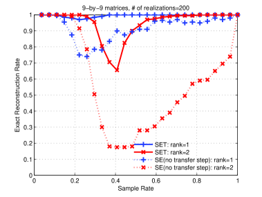
Figure 2: Performance improvement due to the subspace transfer step.

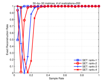
Figure 3: Performance of the SET algorithm.

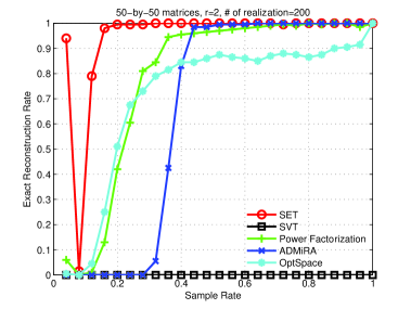
Figure 4: Performance comparison.

Finally, we would like to comment on the complexity of the SET algorithm. The computational complexity is related to the number of iterations required for convergence. Since it incorporates a gradient descent part, the SET algorithm inherits the general disadvantages of a gradient descent approach: the algorithm may take a large number of iterations to converge; within each iteration, finding the optimal step size can be time consuming. Furthermore, extra computations are required for the subspace transfer step. At the current stage, we do not have an accurate analytical estimate of the computational complexity.

-A Proof of the form of the gradient in (7)

Let $\bm{F}_{\bm{U}}$ be the $m\times r$ matrix of partial derivatives, i.e., $\left(\bm{F}_{\bm{U}}\right)_{i,j}=\partial f/\partial\bm{U}_{i,j}$. We first write the objective function via the trace function:

$$f =\left\langle\mathcal{P}_{\Omega}\left(\bm{X}_{\Omega}-\bm{U}\bm{W}_{U}\right),\mathcal{P}_{\Omega}\left(\bm{X}_{\Omega}-\bm{U}\bm{W}_{U}\right)\right\rangle$$

$$\overset{\left(a\right)}{=}\left\langle\bm{X}-\bm{U}\bm{W}_{U},\mathcal{P}_{\Omega}^{*}\left(\mathcal{P}_{\Omega}\left(\bm{X}_{\Omega}-\bm{U}\bm{W}_{U}\right)\right)\right\rangle$$

$$\overset{\left(b\right)}{=}\left\langle\bm{X}-\bm{U}\bm{W}_{U},\mathcal{P}_{\Omega}\left(\bm{X}_{\Omega}-\bm{U}\bm{W}_{U}\right)\right\rangle,$$

$$=\mbox{trace}\left(\left(\bm{X}-\bm{U}\bm{W}_{U}\right)^{T}\mathcal{P}_{\Omega}\left(\bm{X}_{\Omega}-\bm{U}\bm{W}_{U}\right)\right)$$

where the symbol $\mathcal{P}_{\Omega}^{*}$ in $\left(a\right)$ denotes the adjoint operator of $\mathcal{P}_{\Omega}$. Equation $\left(a\right)$ follows from the definition of the adjoint operator, and equation $\left(b\right)$ holds because the operator $\mathcal{P}_{\Omega}$ is self-adjoint and idempotent. Note that

$$\frac{\partial f}{\partial\bm{U}_{i,j}}=\left.\frac{\partial f}{\partial\bm{U}_{i,j}}\right|_{\bm{W}_{U}}+\sum_{k,\ell}\left.\frac{\partial f}{\partial\left(\bm{W}_{U}\right)_{k,\ell}}\right|_{\bm{U}}\frac{\partial\left(\bm{W}_{U}\right)_{k,\ell}}{\partial\bm{U}_{i,j}}.$$

Since $\bm{W}_{U}$ is the solution of the least square problem in (6), we have

$$\left.\frac{\partial f}{\partial\left(\bm{W}_{U}\right)_{k,\ell}}\right|_{\bm{U}}=0,\;\mbox{for all}\;1\leq k\leq r\;\mbox{and}\;1\leq\ell\leq n.$$

Therefore,

$$\bm{F}_{\bm{U}} =\frac{\partial f}{\partial\bm{U}}=\left.\frac{\partial f}{\partial\bm{U}}\right|_{\bm{W}_{U}}$$

$$=-2\mathcal{P}_{\Omega}\left(\bm{X}_{\Omega}-\bm{U}\bm{W}_{U}\right)\bm{W}_{U}^{T}=-2\bm{X}_{r}\bm{W}_{U}^{T}.$$

According to [12, pg. 20], the corresponding tangent vector $\nabla_{\bm{U}}f$ (with respect to the Grassmann manifold) is given by $\nabla_{\bm{U}}f=\bm{F}_{\bm{U}}-\bm{U}\bm{U}^{T}\bm{F}_{\bm{U}}.$ Since $\bm{W}_{U}$ minimizes the Frobenius norm, it is straightforward to verify that $\bm{U}$ is orthogonal to $\bm{X}_{r}$, i.e., $\bm{U}^{T}\bm{X}_{r}=\bm{0}$. Therefore, $\nabla_{\bm{U}}f=\bm{F}_{\bm{U}}=-2\bm{X}_{r}\bm{W}_{U}^{T}$ which proves (7).

-B Proof of the decoupling principle in (10)

Arbitrarily pick a $\bm{U}\in\mathbb{R}^{m\times r}$. For the matrix $\bm{X}_{\Omega}$, the objective function $\left\|\bm{X}_{\Omega}-\mathcal{P}_{\Omega}\left(\bm{U}\bm{W}\right)\right\|_{F}^{2}$ is convex in $\bm{W}$. Let $\bm{W}^{\left(0\right)}$ be a global minimizer for this function. For each column of $\bm{X}_{\Omega}$, say $\bm{x}_{\Omega_{j}}$, the function $\left\|\bm{x}_{\Omega_{j}}-\mathcal{P}_{\Omega_{j}}\left(\bm{U}\bm{W}_{:,j}\right)\right\|^{2}$ is also convex. Let $\bm{W}_{:j}^{\left(1\right)}$ now be the global minimizer for this $j^{th}$ atomic function. Concatenate $\bm{W}_{:1}^{\left(1\right)},\cdots,\bm{W}_{:n_{2}}^{\left(1\right)}$ into a matrix and denote the resulting matrix by $\bm{W}^{\left(1\right)}$. By the additivity of the squared Frobenius norm, the right side of (10) becomes $\left\|\bm{X}_{\Omega}-\mathcal{P}_{\Omega}\left(\bm{U}\bm{W}^{\left(1\right)}\right)\right\|_{F}^{2}$. By the definition of $\bm{W}^{\left(0\right)}$, $\left\|\bm{X}_{\Omega}-\mathcal{P}_{\Omega}\left(\bm{U}\bm{W}^{\left(0\right)}\right)\right\|_{F}^{2}\leq\left\|\bm{X}_{\Omega}-\mathcal{P}_{\Omega}\left(\bm{U}\bm{W}^{\left(1\right)}\right)\right\|_{F}^{2}$. On the other hand,

$$\left\|\bm{X}_{\Omega}-\mathcal{P}_{\Omega}\left(\bm{U}\bm{W}^{\left(1\right)}\right)\right\|_{F}^{2} =\sum_{j=1}^{n_{2}}\left\|\bm{x}_{\Omega_{j}}-\mathcal{P}_{\Omega_{j}}\left(\bm{U}\bm{W}_{:j}^{\left(1\right)}\right)\right\|_{F}^{2}$$

$$\leq\sum_{j=1}^{n_{2}}\left\|\bm{x}_{\Omega_{j}}-\mathcal{P}_{\Omega_{j}}\left(\bm{U}\bm{W}_{:j}^{\left(0\right)}\right)\right\|_{F}^{2}$$

$$=\left\|\bm{X}_{\Omega}-\mathcal{P}_{\Omega}\left(\bm{U}\bm{W}^{\left(0\right)}\right)\right\|_{F}^{2}.$$

This proves equation (10).

-C Determination of Consistency

Let $\bm{G}=\left.\nabla_{\bm{U}}f\right|_{\bm{U}\left(t_{\max,k}\right)}$ be the gradient of $f$ at $\bm{U}\left(t_{\max,k}\right)$. It can be computed via (7). Consider the geodesic curve in (5). Define

$$\bm{H}\left(t\right)=\left[-\bm{u}_{1}\sin t+\bm{h}\cos t,\bm{0},\cdots,\bm{0}\right]\;\mbox{for}\;t\in\left[0,\pi\right).$$

It can be shown that $\bm{H}\left(t_{\max,k}\right)$ is the parallel transportation of $\bm{H}$ at $t_{\max,k}$ (see [12, pg. 19] for more details). Based on the definition of the gradient, it can be shown that $\frac{d}{dt}f\left(\bm{U}\left(t\right)\right)<0$ if and only if

$$\left\langle\bm{G},\bm{H}\left(t_{\max,k}\right)\right\rangle=\bm{G}^{T}\bm{H}\left(t_{\max,k}\right)<0.$$

-D Proof of Proposition 1

This subsection presents the proof of Proposition 1 and the mechanism in Section III-F for computing $t_{\max}$ and $t_{\min}$. We first study the case $r=1$ and then extend the results to the general case where $r>1$.

In the rank-one case, the geodesic curve has the form $\bm{U}\left(t\right)=\bm{u}\cos t+\bm{h}\sin t$, with $t\in\left[0,\pi\right)$. For some $\Omega\subset\left[m\right]$, an atomic function can be written as $\left\|\bm{x}_{\Omega}-\mathcal{P}\left(\bm{x}_{\Omega},\bm{u}_{\Omega}\cos t+\bm{h}_{\Omega}\sin t\right)\right\|^{2}$, where $\bm{u}_{\Omega}=\mathcal{P}_{\Omega}\left(\bm{u}\right)$ and $\bm{h}_{\Omega}=\mathcal{P}_{\Omega}\left(\bm{h}\right)$. Note that $\bm{u}_{\Omega}$ may not be of unit norm. For notational convenience, we drop the subscript $\Omega$. The following proposition describes the general behavior of an atomic function.

Proposition 2

Let $\bm{y},\bm{u}_{1},\bm{u}_{2}\in\mathbb{R}^{m}$. Suppose that

1. The vectors $\bm{u}_{1}$ and $\bm{u}_{2}$ are linearly independent.

2. The vector $\bm{y}$ is not orthogonal to both $\bm{u}_{1}$ and $\bm{u}_{2}$ simultaneously.

Let $\bm{u}\left(t\right)=\bm{u}_{1}\cos t+\bm{u}_{2}\sin t$ where $t\in\mathbb{R}$. Define $\bm{y}_{r}\left(t\right)=\bm{y}-\mathcal{P}\left(\bm{y},\bm{u}\left(t\right)\right)$ and $f\left(t\right)=\left\|\bm{y}_{r}\left(t\right)\right\|^{2}$. Then the following is true.

1. $f\left(t\right)$ is a periodic function with period $\pi$.

2. $f\left(t\right)$ has a unique minimizer $t_{\min}$ and a unique maximizer $t_{\max}$.

3. The maximizer $t_{\max}$ defined in 2) can be computed in the following way. Let $\bm{c}=\left[c_{1},c_{2}\right]^{T}=\mbox{coeff}\left(\bm{y},\left[\bm{u}_{1},\bm{u}_{2}\right]\right)$. Then $t_{\max}=\mbox{atan}\left(c_{2},c_{1}\right)$, where the atan function is defined in (15).

4. The minimizer $t_{\min}$ defined in 2) is computed via $t_{\min}=\mbox{atan}\left(\bm{y}^{T}\bm{u}_{i},-\bm{y}^{T}\bm{u}_{2}\right)$.

Proof:

This first part is proved by observing that $\bm{u}\left(t+\pi\right)=-\bm{u}\left(t\right)$. Note that for a given $t$,

$$\bm{y}_{r}\left(t\right)=\bm{y}-\left(\bm{y}^{T}\bm{u}\left(t\right)/\left\|\bm{u}\left(t\right)\right\|^{2}\right)\bm{u}\left(t\right).$$

One has

$$\bm{y}_{r}\left(t+\pi\right) =\bm{y}-\left(\bm{y}^{T}\bm{u}\left(t+\pi\right)/\left\|\bm{u}\left(t+\pi\right)\right\|^{2}\right)\bm{u}\left(t+\pi\right)$$

$$=\bm{y}-\left(-\bm{y}^{T}\bm{u}\left(t\right)/\left\|\bm{u}\left(t\right)\right\|^{2}\right)\left(-\bm{u}\left(t\right)\right)$$

$$=\bm{y}_{r}\left(t\right).$$

The other claims of this proposition are proved as follows. By assumption, $\bm{u}_{1}$ and $\bm{u}_{2}$ are linearly independent. As a result, $\mbox{span}\left(\left[\bm{u}_{1},\bm{u}_{2}\right]\right)$ is a hyperplane with dimension two. It is clear that $\bm{u}\left(t\right)=\bm{u}_{1}\cos t+\bm{u}_{2}\sin t\neq 0$ for all $t\in\mathbb{R}$ and it forms an ellipse on the hyperplane $\mbox{span}\left(\left[\bm{u}_{1},\bm{u}_{2}\right]\right)$ centered at 0. Any line in the hyperplane $\mbox{span}\left(\left[\bm{u}_{1},\bm{u}_{2}\right]\right)$ through the origin can be uniquely represented by a point on the half ellipse $\bm{u}\left(t\right)$ with $t\in\left[0,\pi\right)$: that is, for all unit vector $\bm{u}^{\prime}\in\mbox{span}\left(\left[\bm{u}_{1},\bm{u}_{2}\right]\right)$, there exists a unique $t\in\left[0,\pi\right)$ and an $s\in\mathbb{R}$ such that $\bm{u}^{\prime}s=\bm{u}\left(t\right)$. In other words, the half ellipse $\bm{u}\left(t\right)$ with $t\in\left[0,\pi\right)$ presents all possible lines (through the origin) in the hyperplane $\mbox{span}\left(\left[\bm{u}_{1},\bm{u}_{2}\right]\right)$.

Let $\bm{y}_{p}$ be the projection of $\bm{y}$ on the hyperplane $\mbox{span}\left(\left[\bm{u}_{1},\bm{u}_{2}\right]\right)$, i.e., $\bm{y}_{p}=\mbox{proj}\left(\bm{y},\left[\bm{u}_{1},\bm{u}_{2}\right]\right)$. It is clear that $f\left(t\right)$ is maximized when $\bm{u}\left(t\right)$ is aligned with $\bm{y}_{p}$: this means, there exists a constant $c\in\mathbb{R}$ such that $\bm{u}\left(t\right)=c\bm{y}_{p}$. By the definition of the projection, we have $\bm{y}_{p}=\left[\bm{u}_{1},\bm{u}_{2}\right]\bm{c}=\bm{u}_{1}c_{1}+\bm{u}_{2}c_{2}$. Therefore, $t_{\max}=\mbox{atan}\left(c_{2},c_{1}\right)$.

The function $f\left(t\right)$ is minimized when $\bm{u}\left(t\right)$ is orthogonal to $\bm{y}$. We have $\bm{y}^{T}\bm{u}_{1}\cos t_{\min}+\bm{y}^{T}\bm{u}_{2}\sin t_{\min}=0$. Solving this equation proves part 4.

We prove the uniqueness results next. By assumption, $\bm{y}$ is not orthogonal to both $\bm{u}_{1}$ and $\bm{u}_{2}$ simultaneously. Hence, $\bm{y}_{p}\neq 0$. Furthermore, since $\bm{u}_{1}$ and $\bm{u}_{2}$ are linearly independent, the vector $\bm{y}_{p}$ is uniquely defined. This establishes the uniqueness of $t_{\max}$. Since the dimension of the hyperplane $\mbox{span}\left(\left[\bm{u}_{1},\bm{u}_{2}\right]\right)$ is two, there exists a unique line in $\mbox{span}\left(\left[\bm{u}_{1},\bm{u}_{2}\right]\right)$ to be orthogonal to $\bm{y}_{p}\in\mbox{span}\left(\left[\bm{u}_{1},\bm{u}_{2}\right]\right)$. We denote this line by a vector $\bm{y}_{\perp}\neq 0$, such that $\bm{y}_{\perp}\in\mbox{span}\left(\left[\bm{u}_{1},\bm{u}_{2}\right]\right)$ and $\bm{y}_{\perp}^{T}\bm{y}_{p}=0$. First, $\bm{y}_{\perp}$ is orthogonal to $\bm{y}$. This can be easily verified as $\bm{y}=\bm{y}_{p}+\bm{y}_{r}$, where $\bm{y}_{r}$ is the projection residue vector and therefore is orthogonal to $\bm{y}_{\perp}$ as well. Second, any linear combination of $\bm{y}_{\perp}$ and $\bm{y}_{p}$ such that the coefficient of $\bm{y}_{p}$ is nonzero produces a line that is not orthogonal to $\bm{y}$. Therefore, $\bm{y}_{\perp}$ represents the unique line in $\mbox{span}\left(\left[\bm{u}_{1},\bm{u}_{2}\right]\right)$ that is orthogonal to $\bm{y}$. The corresponding value $t_{\min}$ is therefore unique. ∎

We proceed next with the general case where $r\geq 1$. Recall the expression for the geodesic curve in (5). Denote $\mathcal{P}_{\Omega}\left(\bm{h}\right)$ by $\bm{h}_{\Omega}$. Similarly, we have $\bm{u}_{1,\Omega},\cdots,\bm{u}_{r,\Omega}$. Let $\bm{u}_{1,\Omega}\left(t\right)=\bm{u}_{1,\Omega}\cos t+\bm{h}_{\Omega}\sin t$. The atomic function can be written as

$$f\left(t\right)=\left\|\bm{x}_{\Omega}-\mathcal{P}\left(\bm{x}_{\Omega},\left[\bm{u}_{1,\Omega}\left(t\right),\bm{u}_{2,\Omega},\cdots,\bm{u}_{r,\Omega}\right]\right)\right\|_{F}^{2}.$$

Again we drop the subscript $\Omega$ for convenience. The following proposition is the key to understand the relationship between $\mathcal{P}\left(\bm{x},\bm{u}_{1}\left(t\right)\right)$ and $\mathcal{P}\left(\bm{x},\left[\bm{u}_{1}\left(t\right),\bm{u}_{2},\cdots,\bm{u}_{r}\right]\right)$.

Proposition 3

Let $\bm{y}\in\mathbb{R}^{m}$, $\bm{U}_{1}\in\mathbb{R}^{m\times n_{1}}$ and $\bm{U}_{2}\in\mathbb{R}^{m\times n_{2}}$ where $n_{1},n_{2}\in\left[m\right]$. Let

$$\bm{y}_{r}=\bm{y}-\mathcal{P}\left(\bm{y},\left[\bm{U}_{1},\bm{U}_{2}\right]\right).$$

Denote the $j^{th}$ column of $\bm{U}_{2}$ by $\left(\bm{U}_{2}\right)_{:j}$. Then $\bm{y}_{r}$ can be written as

$$\bm{y}_{r}=\bm{y}_{r,1}-\mathcal{P}\left(\bm{y}_{r,1},\bm{U}_{2,r}\right),$$

where $\bm{y}_{r,1}=\mathcal{P}\left(\bm{y},\bm{U}_{1}\right)$, and $\bm{U}_{2,r}=\left[\left(\bm{U}_{2}\right)_{:1}-\mathcal{P}\left(\left(\bm{U}_{2}\right)_{:1},\bm{U}_{1}\right),\cdots,\left(\bm{U}_{2}\right)_{:r}-\mathcal{P}\left(\left(\bm{U}_{2}\right)_{:r},\bm{U}_{1}\right)\right]$.

Proof:

The proof is centered around the notion of projection. For arbitrary $\bm{y}\in\mathbb{R}^{m}$ and $\bm{U}\in\mathbb{R}^{m\times n}$, an operator $\mathcal{P}$ is a projection operator if and only if $\mathcal{P}\left(\bm{y},\bm{U}\right)\in\mbox{span}\left(\bm{U}\right)$ and $\bm{y}_{r}\perp\bm{U}$, where $\bm{y}_{r}=\bm{y}-\mathcal{P}\left(\bm{y},\bm{U}\right)$. We say $\bm{y}_{r}\perp\bm{U}$ if $\bm{y}_{r}^{T}\bm{U}_{:j}=0$ for all $j\in\left[n\right]$.

Let $\bm{y}^{\prime}=\bm{y}_{r,1}-\mathcal{P}\left(\bm{y}_{r,1},\bm{U}_{2,r}\right)$. To prove this proposition, it suffices to show that $\bm{y}_{r}^{\prime}\perp\left[\bm{U}_{1},\bm{U}_{2}\right]$ and $\bm{y}-\bm{y}_{r}^{\prime}\in\mbox{span}\left(\left[\bm{U}_{1},\bm{U}_{2}\right]\right)$.

We first show that $\bm{y}_{r}^{\prime}\perp\left[\bm{U}_{1},\bm{U}_{2}\right]$. That $\bm{y}_{r}^{\prime}\perp\bm{U}_{1}$ is verified as follows. Since $\mathcal{P}\left(\bm{y}_{r,1},\bm{U}_{2,r}\right)\in\mbox{span}\left(\bm{U}_{2,r}\right)$ and each column of $\bm{U}_{2,r}$ is orthogonal to $\bm{U}_{1}$, we have $\mathcal{P}\left(\bm{y}_{r,1},\bm{U}_{2,r}\right)\perp\bm{U}_{1}$. The definition of $\bm{y}_{r,1}$ implies that $\bm{y}_{r,1}\perp\bm{U}_{1}$. Hence, we have $\bm{y}_{r}^{\prime}\perp\bm{U}_{1}$ as the vector $\bm{y}_{r}^{\prime}$ is a linear combination of $\bm{y}_{r,1}$ and $\mathcal{P}\left(\bm{y}_{r,1},\bm{U}_{2,r}\right)$. We claim that $\bm{y}_{r}^{\prime}\perp\bm{U}_{2}$ as well. According to the definition of $\bm{y}_{r}^{\prime}$, it is clear that $\bm{y}_{r}^{\prime}\perp\bm{U}_{2,r}$. Note that $\left(\bm{U}_{2}\right)_{:j}=\left(\bm{U}_{2,r}\right)_{:j}+\mathcal{P}\left(\left(\bm{U}_{2}\right)_{:j},\bm{U}_{1}\right)$. The vector $\mathcal{P}\left(\left(\bm{U}_{2}\right)_{:j},\bm{U}_{1}\right)$ is in the $\mbox{span}\left(\bm{U}_{1}\right)$ and therefore orthogonal to $\bm{y}_{r}^{\prime}$. As a result, $\bm{y}_{r}^{\prime}\perp\bm{U}_{2}$. We then have $\bm{y}_{r}^{\prime}\perp\left[\bm{U}_{1},\bm{U}_{2}\right]$.

Next, we show that $\bm{y}-\bm{y}_{r}^{\prime}\in\mbox{span}\left(\left[\bm{U}_{1},\bm{U}_{2}\right]\right)$. Note that

$$\bm{y}-\bm{y}_{r}^{\prime} =\bm{y}-\bm{y}_{r,1}+\mathcal{P}\left(\bm{y}_{r,1},\bm{U}_{2,r}\right)$$

$$=\mathcal{P}\left(\bm{y},\bm{U}_{1}\right)+\mathcal{P}\left(\bm{y}_{r,1},\bm{U}_{2,r}\right).$$

Clearly, $\mathcal{P}\left(\bm{y},\bm{U}_{1}\right)\in\mbox{span}\left(\bm{U}_{1}\right)\subset\mbox{span}\left(\left[\bm{U}_{1},\bm{U}_{2}\right]\right)$. Furthermore, according to the definition of $\bm{U}_{2,r}$, $\mbox{span}\left(\bm{U}_{2,r}\right)\subset\mbox{span}\left(\left[\bm{U}_{1},\bm{U}_{2}\right]\right)$ and therefore $\mathcal{P}\left(\bm{y}_{r,1},\bm{U}_{2,r}\right)\in\mbox{span}\left(\bm{U}_{2,r}\right)\subset\mbox{span}\left(\left[\bm{U}_{1},\bm{U}_{2}\right]\right)$. This completes the proof. ∎

Based on the claim of this proposition, one can to apply the analysis for the rank-one case (Proposition 2) to higher-rank cases. Let $\bm{U}_{\sim 1}=\left[\bm{u}_{2},\cdots,\bm{u}_{r}\right]$, and let $\bm{x}_{r}=\bm{x}-\mathcal{P}\left(\bm{x},\bm{U}_{\sim 1}\right)$. Similarly, define $\bm{u}_{1,r}$ and $\bm{h}_{r}$. It is clear that

$$\bm{u}_{1,r}\left(t\right) =\bm{u}_{1}\left(t\right)-\mathcal{P}\left(\bm{u}_{1}\left(t\right),\bm{U}_{\sim 1}\right)$$

$$=\bm{u}_{1}\cos t+\bm{h}\sin t$$

$$\quad-\mathcal{P}\left(\bm{u}_{1},\bm{U}_{\sim 1}\right)\cos t-\mathcal{P}\left(\bm{h},\bm{U}_{\sim 1}\right)\sin t$$

$$=\bm{u}_{1,r}\cos t+\bm{h}_{r}\sin t.$$

One has

$$\bm{x}-\mathcal{P}\left(\bm{x},\left[\bm{u}_{1}\left(t\right),\bm{u}_{2},\cdots,\bm{u}_{r}\right]\right)$$

$$=\bm{x}_{r}-\mathcal{P}\left(\bm{x}_{r},\bm{u}_{1,r}\left(t\right)\right).$$

This establishes the connection between the rank-one case and the general case, proves Proposition 1, and justifies the procedure in Section III-F for computing minimizers and maximizers.

References

• [1] E. Candes and B. Recht, “Exact matrix completion via convex optimization,” arXiv:0805.4471, 2008.
• [2] E. J. Candes and T. Tao, “The power of convex relaxation: Near-optimal matrix completion,” arXiv:0903.1476, Mar. 2009.
• [3] J. Cai, E. J. Candes, and Z. Shen, “A singular value thresholding algorithm for matrix completion,” arXiv:0810.3286, 2008.
• [4] E. J. Candès, X. Li, Y. Ma, and J. Wright, “Robust principal component analysis?,” arXiv:0912.3599, 2009.
• [5] K. Lee and Y. Bresler, “ADMiRA: atomic decomposition for minimum rank approximation,” arXiv:0905.0044, Apr. 2009.
• [6] W. Dai and O. Milenkovic, “Subspace pursuit for compressive sensing signal reconstruction,” IEEE Trans. Inform. Theory, vol. 55, pp. 2230 – 2249, May 2009.
• [7] D. Needell and J. A. Tropp, “CoSaMP: Iterative signal recovery from incomplete and inaccurate samples,” Applied and Computational Harmonic Analysis, vol. 26, pp. 301–321, May 2009.
• [8] R. Meka, P. Jain, and I. S. Dhillon, “Guaranteed rank minimization via singular value projection,” arXiv:0909.5457, 2009.
• [9] T. Blumensath and M. E. Davies, “Iterative hard thresholding for compressed sensing,” Applied and Computational Harmonic Analysis, vol. 27, pp. 265–274, Nov. 2009.
• [10] J. Haldar and D. Hernando, “Rank-constrained solutions to linear matrix equations using powerfactorization,” IEEE Signal Processing Letters, pp. 16:584–587, 2009.
• [11] R. H. Keshavan, A. Montanari, and S. Oh, “Matrix completion from a few entries,” arXiv:0901.3150, 2009.
• [12] A. Edelman, T. Arias, S. T. Smith, Steven, and T. Smith, “The geometry of algorithms with orthogonality constraints,” SIAM Journal on Matrix Analysis and Applications, vol. 20, pp. 303–353, April 1999.
• [13] P. E. Gill, W. Murray, and M. H. Wright, Practical Optimization. Academic Press, 1982.