Extraction of Electromagnetic Transition Form Factors for Nucleon Resonances within a Dynamical Coupled-Channels Model

Abstract

We explain the application of a recently developed analytic continuation method to extract the electromagnetic transition form factors for the nucleon resonances ($N^{*}$) within a dynamical coupled-channel model of meson-baryon reactions. Illustrative results of the obtained $N^{*}\rightarrow\gamma N$ transition form factors, defined at the resonance pole positions on the complex energy plane, for the well isolated $P_{33}$ and $D_{13}$, and the complicated $P_{11}$ resonances are presented. A formula has been developed to give an unified representation of the effects due to the first two $P_{11}$ poles, which are near the $\pi\Delta$ threshold, but are on different Riemann sheets. We also find that a simple formula, with its parameters determined in the Laurent expansions of $\pi N\rightarrow\pi N$ and $\gamma N\rightarrow\pi N$ amplitudes, can reproduce to a very large extent the exact solutions of the considered model at energies near the real parts of the extracted resonance positions. We indicate the differences between our results and those extracted from the approaches using the Breit-Wigner parametrization of resonant amplitudes to fit the data.

I Introduction

The spectrum and form factors of excited nucleons are fundamental quantities for investigating the hadron structure within Quantum Chromodynamics (QCD). The excited nucleons are unstable and couple strongly to meson-baryon continuum states to form nucleon resonances (called collectively as $N^{*}$) in $\pi N$ and $\gamma N$ reactions. It is well known that resonances locate on the unphysical sheets of complex energy plane and thus their properties can only be extracted from the empirical partial-wave amplitudes by analytic continuation. Recently we have applied an analytic continuation method developed in Ref.ssl09 to extract $N^{*}$ pole positionssjklms10 from $\pi N$ elastic scattering amplitudes determined in a fitjlms07 (JLMS) within a dynamical coupled channel modelmsl07 (EBAC-DCC) of meson-baryon reactions.

The scattering amplitudes obtained from a dynamical coupled-channels model of meson-baryon reactions, such as the EBAC-DCC model as well as the models developed in Refs.afnan ; gross ; sl96 ; ntuanl ; juelich-0 , are not available in an analytic form. They are obtained numerically by solving coupled-channels integral equations with meson-exchange driving terms. Thus, the predicted amplitudes can only be analytically continued to complex energy plane numerically with a careful account of the analytic structure of the considered scattering equations. Obviously, the method depends on the dynamical content of each model. For EBAC-DCC model, this has been developed in Ref.ssl09 and established using several exactly soluble models. In this paper, we explain how this method is used to extract $\gamma^{*}N\rightarrow N^{*}$ transition form factors from the multipole amplitudes determined from extending the JLMS analysis to investigate $\gamma N\rightarrow\pi N$jlmss08 and $N(e,e^{\prime}\pi)N$jklmss09 reactions.

The electromagnetic $\gamma^{*}N\rightarrow N^{*}$ transition form factors give information on the current and charge distributions of $N^{*}$ and $N$. It can be shownbohm ; dalitz that a resonance state $|\psi^{R}_{N^{*}}>$ with a complex energy $M_{R}$ can be defined as an ’eigenstate’ of Hamiltonian $H|\psi^{R}_{N^{*}}>=M_{R}|\psi^{R}_{N^{*}}>$ with the outgoing boundary condition for its asymptotic wave functions. Therefore the $\gamma^{*}N\rightarrow N^{*}$ transition form factor is defined by the current matrix element $<\psi^{R}_{N^{*}}|J_{em}|N>$ which can be extracted from the residue $R_{\pi N,\gamma^{*}N}$ of electromagnetic pion production amplitudes at the resonance poles. To extract $R_{\pi N,\gamma^{*}N}$, we need to evaluate the on-shell matrix elements of $\gamma^{*}N\rightarrow\pi N$ amplitudes on the complex Riemann energy sheet. As will be discussed later, the analytic structure of the considered coupled-channels equations for getting these on-shell matrix elements is rather complex and must be dealt with carefully. In particular, we need to develop a formula to give an unified representation of the first two $P_{11}$ resonances which are near the $\pi\Delta$ threshold, but are on different Riemann sheets.

To illustrate our approach, it is sufficient to only present results for the well isolated resonances in $P_{33}$ and $D_{13}$ and the complex $P_{11}$ partial waves. With only three complex parameters determined in the Laurent expansion of each partial-wave amplitude at resonance pole position, we present a simple formula which can reproduce to a very large extent the exact solutions of the considered model at energies near the real parts of the extracted resonance positions. This finding agrees with what was reported in an analysisjuelich of $\pi N$ scattering amplitude within the Jülich modeljuelich-0 . Here we show that this formula is also a good approximation for $\gamma N\rightarrow\pi N$ amplitudes. Despite that this formula is similar to that used in the analysisgwu-vpi ; maid ; inna using the Breit-Wigner parametrization of resonant amplitudes to fit the data, we find no simple relation between two approaches.

In section II, we will briefly review the analytic continuation method developed in Ref.ssl09 and explain how it is applied to evaluate the on-shell amplitudes of $\pi N,\gamma^{*}N\rightarrow\pi N$ transitions. Section III is devoted to explaining how the determined residues are used to extract the elasticity $\eta_{el}$ of $N^{*}\rightarrow\pi N$ decay and the $\gamma^{*}N\rightarrow N^{*}$ transition form factors at resonance poles. The results for $P_{11}$, $P_{33}$, and $D_{13}$ nucleon resonances are presented in section IV. A summary is given in section V.

II Analytic continuation method

Within the formulationmsl07 for EBAC-DCC model, the partial wave amplitudes of meson-baryon reactions can be written as

$$T_{\beta,\alpha}(p^{\prime},p;E) = t_{\beta,\alpha}(p^{\prime},p;E)+t^{R}_{\beta,\alpha}(p^{\prime},p;E)\,,$$ (1)

where $\alpha,\beta$ represent the meson-baryon (MB) states $\gamma N$, $\pi N,\eta N,\rho N,\sigma N,\pi\Delta$, and

$$t^{R}_{\beta,\alpha}(p^{\prime},p;E) = \sum_{i,j}\bar{\Gamma}_{\beta,i}(p^{\prime};E)[G_{N^{*}}(E)]_{i,j}\bar{\Gamma}_{\alpha,j}(p;E)$$ (2)

with

$$[G_{N^{*}}^{-1}]_{i,j}(E) = (E-m_{N^{*}_{i}})\delta_{i,j}-\Sigma_{i,j}(E)\,.$$ (3)

Here $i,j$ denote the bare $N^{*}$ states defined in the Hamiltonian. $m_{N^{*}_{i}}$ are their masses. The first term (called meson-exchange amplitude from now on) in Eq.(1) is defined by the following coupled-channels equation

$$t_{\beta,\alpha}(p^{\prime},p;E) = v_{\beta,\alpha}(p^{\prime},p)+\int_{C}dqq^{2}\sum_{\gamma}v_{\beta,\gamma}(p^{\prime},q;E)G_{\gamma}(q,E)t_{\gamma,\alpha}(q,p;E)$$ (4)

where $v_{\beta,\alpha}$ is defined by meson-exchange mechanisms, and $G_{\gamma}(q,E)$ is the propagator for channel $\gamma$. The dressed vertexes and the energy shifts of the second term in Eqs.(2)-(3) are defined by

$$\bar{\Gamma}_{\alpha,j}(p;E) = \Gamma_{\alpha,j}(p)+\int_{C}dqq^{2}\sum_{\gamma}t_{\alpha,\gamma}(p^{\prime},q;E)G_{\gamma}(q,E)\Gamma_{\gamma,j}(q)$$ (5)

$$\Sigma(E)_{i,j} = \int_{C}dqq^{2}\sum_{\gamma}\Gamma_{\gamma,i}(q)G_{\gamma}(q,E)\bar{\Gamma}_{\gamma,j}(q),$$ (6)

where $\Gamma_{\alpha,i}(p)$ defines the coupling of the $i$-th bare $N^{*}$ state to channel $\alpha$.

Because of the quadratic relation between energy $E$ and momentum $p$, there are two energy sheets for each two-body channel: the physical (unphysical) sheet is identified with $Im(p)>(<)$ 0 for the stable two-particle channels. Thus the scattering amplitudes of an $n$-channels model are defined on a Riemann energy sheet which consists of $2^{n}$ sheets. For the EBAC-DCC model, defined by Eqs.(1)-(6), each sheet can be defined by symbol $(z_{\pi N},z_{\eta N},z_{\pi\pi N},z_{\pi\Delta},z_{\rho N},z_{\sigma N})$ , where $z_{\alpha}$ could be $p$ or $u$ representing the physical or unphysical sheets of channel $\alpha$. Note that an acceptable reaction model can only have bound state poles and unitarity cuts on the physical sheet $(pppppp)$. The sheets from all other possible combinations of $u$ and $p$ are called unphysical sheets on which the scattering amplitude can have poles. We are however only interested in poles which have large effects on scattering observables and therefore they must be on the sheets which are near the $(pppppp)$ physical sheet. These poles are called resonance poles, and other poles are called shadow poles. It is knowntaylor ; mp87 that a shadow pole near the threshold of a channel can also have large effects on scattering observables and must also be considered in the search. As analyzed in Ref.ssl09 using several exactly soluble models, these poles are in most cases on sheets where the open(above threshold) meson-baryon channels are on unphysical $u$ sheets and the closed(below threshold) channels are on physical sheet. In below we first recall how the analytic continuation method we had developed in Ref.ssl09 is used to search for such resonance poles within EBAC-DCC model. We then describe how it is used to extract the residues of the extracted resonance poles from on-shell amplitudes.

Since $v_{\alpha,\beta}$ and the bare vertex $\Gamma_{\alpha,i}$ are energy independent within the EBAC-DCC model , the analytic structure of the scattering amplitude defined above as a function of $E$ is mainly determined by the Green functions $G_{\gamma}(q,E)$. Thus the key for selecting the amplitude on physical sheet or unphysical sheet is to take an appropriate path of momentum integration $C$ in Eqs.(1)-(6) according to the locations of the singularities of the meson-baryon Green functions $G_{\alpha}(p,E)$ as $E$ moves to complex plane. This can be done independently for each meson-baryon channel. For channel with stable particles such as $\pi N$ and $\eta N$, the meson-baryon Green function is

$$G_{MB}(E,p)=\frac{1}{E-E_{M}(p)-E_{B}(p)}\,,$$ (7)

which has a pole at the on-shell momentum $p_{0}$ defined by

$$E=\sqrt{m_{M}^{2}+p^{2}_{0}}+\sqrt{m_{B}^{2}+p^{2}_{0}}.$$ (8)

As an example, let us consider the analytic continuation of the amplitude to the unphysical sheet of the $MB$ channel when the energy $E$ is above the threshold $Re(E)>m_{B}+m_{M}$ and $Im(E)<0$. The on-shell momentum $p_{0}$ for such a $E$ is on the second and the fourth quadrant of the complex momentum plane. As $Im(E)$ becomes more negative as illustrated in Fig. 1, the on-shell momentum (open circle) moves into the fourth quadrant. The amplitude on the unphysical sheet can be obtained by deforming the path $C$ into $C_{1}$ so that the on-shell momentum does not cross the integration contour. For energy below the threshold for the MB channel ($E<m_{B}+m_{M}$), the on-shell momentum $p_{sub}$ is on the axis of positive imaginary. As the energy moves into the region of $Re(E)<m_{B}+m_{M}$ and $Im(E)<0$, $p_{sub}$ moves to the second quadrant of complex p-plane and does not cross path $C_{1}$, as indicated by the dotted curves in Fig.1. Hence the amplitudes on the physical sheet of $MB$ channel for energy below $MB$ threshold can also be obtained by taking the path $C_{1}$.

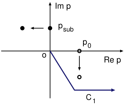
Figure 1: The shift of the on-shell momentum (open circle/solid circle) of the two-particle Green function Eq. (7) as energy E moves from a real value above/below the threshold energy to a complex value with negative imaginary part. $C^{\prime}_{1}$ is the integration path for calculating Eqs.(4)-(6) amplitude for E on the unphysical Riemann sheet.

For the channels with unstable particle such as the $\pi\Delta$, as an example, the Green function is of the following form

$$G_{\pi\Delta}(E,p)=\frac{1}{E-E_{\pi}(p)-E_{\Delta}(p)-\Sigma_{\Delta}(E,p)},$$ (9)

where

$$\Sigma_{\Delta}(p,E)=\int_{C_{3}}\frac{\{\Gamma_{\Delta,\pi N}(q)\}^{2}q^{2}dq}{E-E_{\pi}(p)-[(E_{\pi}(q)+E_{N}(q))^{2}+p^{2}]^{1/2}}.$$

(10)

The $\pi\Delta$ Green function Eq. (9) has a singularity at momentum $p=p_{x}$, which satisfies

$$E-E_{\pi}(p_{x})-E_{\Delta}(p_{x})-\Sigma_{\Delta}(p_{x},E)=0.$$ (11)

Physically, this singularity corresponds to the $\pi\Delta$ two-body ’scattering state’. There is also a discontinuity of the $\pi\Delta$ Green function associated with the $\pi\pi N$ cut in $\Sigma_{\Delta}$, as shown in the dashed line in Fig. 2, where $p_{0}$ is defined by

$$E=E_{\pi}(p_{0})+[(m_{\pi}+m_{N})^{2}+p^{2}_{0}]^{1/2}.$$ (12)

Therefore, for $Re(E)>m_{B}+m_{M},2m_{\pi}+m_{N}$, the integration contour $C$ must be chosen to be below the $\pi\pi N$ cut (dashed line) and the singularity $p_{x}$, such as the contour $C_{2}$ shown in Fig.2, for calculating amplitudes on the unphysical sheet.

The singularity $q_{0}$ of the integrand of Eq. (10) depends on the spectator momentum $p$

$$E-E_{\pi}(p)=[(E_{\pi}(q_{0})+E_{N}(q_{0}))^{2}+p^{2}]^{1/2}\,.$$ (13)

Thus $q_{0}$ moves along the dashed curve, illustrated in Fig.3, when the momentum $p$ varies along the path $C_{2}$ of Fig.2. To analytically continue $\Sigma_{\Delta}(p,E)$ to the unphysical sheet, the contour $C_{3}$ of Eq. (10) must be below $q_{0}$. A possible contour $C_{3}$ is the solid curve in Fig.3.

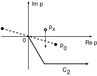
Figure 2: Contour $C_{2}$ for calculating Eqs.(4)-(6) for E on the unphysical Riemann sheet with the unstable particle propagators, such as Eq.(9) for $\pi\Delta$ channel. See the text for the explanations of the dashed line and the singularity $p_{x}$.

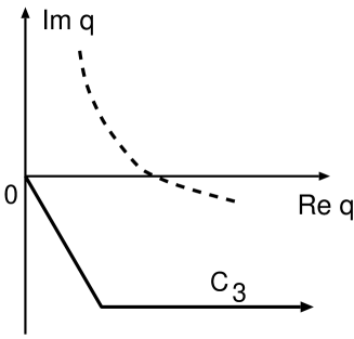
Figure 3: Contour $C_{3}$ for calculating the $\Delta$ self energy Eq.(10) on the unphysical Riemann sheet. Dashed curve is the singularity $q_{0}$ of the propagator in Eq. (13), which depends on the spectator momentum $p$ on the contour $C_{2}$ of Fig.2.

We emphasize here that we can deform the contour $C$ only in the region where the potential $v_{\alpha,\beta}(p^{\prime},p)$ and the bare $N^{*}$ vertex $\Gamma_{MB,N^{*}}(p)$ are analytic. The contours described above are chosen only from considering the singularities of $MB$ and $\pi\pi N$ Green functions. Thus they must be further modified according to the analytic structure of the considered $v_{\alpha,\beta}(p^{\prime},p)$ and $\Gamma_{MB,N^{*}}(p)$ to obtain the scattering amplitude in the momentum region of interest. This consideration is specially necessary when we need to get the on-shell amplitude for extracting the residues of the identified resonance poles. The residue of the amplitude at resonance pole is evaluated from the ’on-shell’ matrix element, where the on-shell momenta are defined as $M_{R}=E_{\pi}(p^{on}_{\pi N})+E_{N}(p^{on}_{\pi N})$ for $\pi N$ channel and $M_{R}=q^{0,on}_{\gamma N}+E_{N}(q^{on}_{\gamma N})$ with $Q^{2}=(q^{on}_{\gamma N})^{2}-(q^{0,on}_{\gamma N})^{2}$ for $\gamma^{*}N$ channel. Since on-shell momentum are in general closer to the real axis than momentum on contour $C$, the analytic properties of the meson-exchange potential has to be examined. For example, the t-channel meson exchange potential $v^{t}_{M^{\prime}B^{\prime},MB}(\vec{p}^{\,\,{}^{\prime}},\vec{p})$ of the EBAC-DCC model has singularities at

$$\Delta^{2}-(\vec{p}-\vec{p}^{\prime})^{2}=0$$ (14)

with $\Delta=E_{M^{\prime}}(p^{\prime})-E_{M}(p)$ or $E_{B^{\prime}}(p^{\prime})-E_{B}(p)$. The form of $\Gamma_{MB,N^{*}}(p)$ is chosen such that its singularity is at the pure imaginary momentum. Thus the contours have to be chosen to also avoid these singularities. As an example we show in Fig.4 the singularities associated with the $\pi\Delta$ channel at $E=(1357,-76i)$ MeV. The dotted line for $\pi\pi N$ cut and the circle shows $p_{X}$ are the singularities from the Green’s function, as discussed above. The most relevant singularity of the meson-exchange potential in our investigation of electromagnetic pion production amplitude is due to the t-channel pion exchange of $\gamma N\rightarrow\pi\Delta$, which is shown as the dashed-dot curve. Thus the integration contour has to be modified to the solid curve $C_{2}$ in Fig.4. This can be understood from Fig. 5 in which we see that the matrix element (dashed curves) of non-resonant potential $v_{\pi\Delta,\gamma N}$ encounters the cut around $Re(p)\sim 170MeV$ with the path $C_{2}^{\prime}$, but it varies smoothly (solid curves) along the path $C_{2}$.

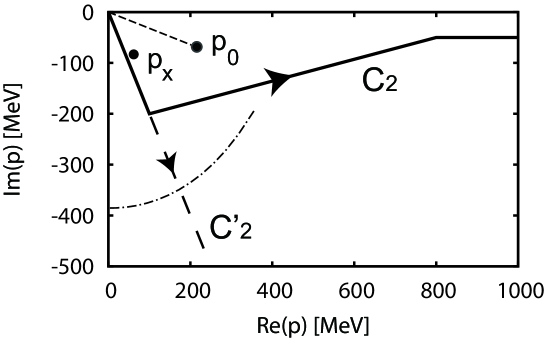
Figure 4: The contour (solid curve) for calculating electromagnetic matrix element. $p_{0}$ and $p_{x}$ are the singularities shown in Fig.2. The dashed-dot curve is the singularity of the pion-exchange $\gamma N\rightarrow\pi\Delta$ matrix element at $E=(1357,-76i)$ MeV.

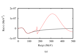
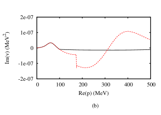
Figure 5: The real (left) and the imaginary(right) parts of the half-off-shell matrix-elements of the non-resonant potential $v_{\gamma N\rightarrow\pi\Delta}$ for $P_{11}$ partial wave at $E=(1357,-76i)$, as functions of the real part ($Re(p)$) of off-shell momentum. The solid(dashed) curve is from the calculation along the path $C_{2}$ ($C_{2}^{\prime}$) shown in Fig.4.

III Extraction of Transition Form Factors

To indicate the essential features of our approach more clearly, it is useful to first briefly describe how the resonance parameters are defined in the previous investigations. The scattering amplitude $F_{\beta,\alpha}$ between any two channels $\alpha$ and $\beta$ is related to the $S$-matrix element by $F_{\beta,\alpha}=(1-S_{\beta,\alpha})/2i$. Within the rather general theoretical framework discussed by, for example, Dalitz and Moorhousedalitz , Taylortaylorbook , and McVoymcvoy , $F_{\beta,\alpha}$ at energies near a resonance pole position $M_{R}$ is parametrized as a sum of a pole term and a constant non-resonant contribution

$$F_{\beta,\alpha}(E\rightarrow M_{R})\sim\frac{R_{\beta,\alpha}}{M_{R}-E}+B_{\beta,\alpha},$$ (15)

where $R_{\beta,\alpha}$ is the residue at the pole position $M_{R}$, and the non-resonant amplitude $B_{\beta,\alpha}$ is an energy independent complex number. By the unitarity condition imposed on the full $S$ matrix $F_{\alpha,\beta}(E)$ at $E\rightarrow M_{R}$, the non-resonant term $B_{\alpha,\beta}$ is written in terms of an non-resonant S-matrix $S^{B}$, which is unitary by itself ($S^{B}S^{B\dagger}=1$)

$$B_{\beta,\alpha} = \frac{1-S^{B}_{\beta,\alpha}}{2i}.$$ (16)

Then the pole term of Eq.(15) is defined by the partial width $\Gamma_{\alpha}$ and a phase $\phi_{\alpha}$ arising from the presence of the non-resonant term $B_{\alpha,\beta}$

$$\frac{R_{\beta,\alpha}}{E-E_{R}} = \frac{e^{i\phi_{\beta}}\sqrt{\Gamma_{\beta}/2}e^{i\phi_{\alpha}}\sqrt{\Gamma_{\alpha}/2}}{E-M_{R}}.$$ (17)

It is important to note that for the $\gamma N\rightarrow\pi N$ amplitudes we are going to consider, $e^{i\phi_{\gamma N}}\sqrt{\Gamma_{\gamma N}}$ is the electromagnetic $\gamma N\rightarrow N^{*}$ form factor which clearly must be a complex number when the the non-resonant term $B_{\pi N,\gamma N}$ is present and $\phi_{\gamma N}\neq 0$. We will see that our formula are consistent with these earlier investigations and will yield complex $\gamma N\rightarrow N^{*}$ form factors. Our main advance is to provide their interpretations in terms of dynamics defined within the EBAC-DCC model.

Here we mention that by introducing appropriate energy-dependence of $Im(M_{R})$, $R_{\alpha\beta}$, and $B_{\alpha,\beta}$, the expression Eq.(15) is used in practice to fit the experimental data. This is the origin of the commonly used Breit-Wigner parametrization of the amplitude in physical energy region. In some recent analysisgwu-vpi ; maid ; inna based on such a Breit-Wigner parametrization, the extracted $\gamma^{*}N\rightarrow N^{*}$ form factors are reported as real numbers. Clearly, this is rather different from what one can interpret from the above formula used in the earlier analysisdalitz ; taylorbook ; mcvoy .

We now explain that within the EBAC-DCC model, it is straightforward to extract the resonance parameters $M_{R}$, $B_{\alpha,\beta}$ and $R_{\alpha,\beta}$ of Eq.(15) by performing a Laurent expansion of the T-matrix defined Eqs.(1)-(6). We need to find poles of scattering amplitudes $T_{\alpha,\beta}$. In principle the pole of the scattering amplitude can be found in the meson-exchange amplitude $t$ and/or resonance amplitude $t^{R}$ of Eq. (1). However as pointed out in Ref. juelich , a pole $M_{x}$ of the meson-exchange amplitude $t$ does not survive as a pole of the full amplitude when we introduce coupling with bare $N^{*}$ states, since there is an exact cancellation between the pole contributions from $t$ and $t^{R}$ at $E=M_{x}$. Furthermore the non-resonant term at resonance pole $t(E=M_{R})$ is finite. Thus, the resonance poles of EBAC-DCC, or any model with bare $N^{*}$ states, can be found by only analyzing $t^{R}$ defined by Eq.(2). Consequently, we only need to explain how the residues of resonance poles are extracted from the term $t^{R}$.

The pole positions $M_{R}$ of $t^{R}$ are found from the zeros of the determinant of $N^{*}$ propagator defined by Eq.(3)

$$\Delta(E=M_{R})=det[G_{N^{*}}^{-1}(E=M_{R})] = 0\,.$$ (18)

The pole term of the $N^{*}$ Green function can be expressed as

$$(G_{N^{*}}(E))_{ij} = \frac{\chi_{i}\chi_{j}}{E-M_{R}}\,,$$ (19)

where $i,j$ denote the bare $N^{*}$ state in the free Hamiltonian and $\chi_{i}$ represents $i$-th ’bare’ resonance component of the dressed $N^{*}$ and satisfies

$$\sum_{j}(G_{N^{*}}(M_{R})^{-1})_{ij}\chi_{j} = \sum_{j}[(M_{R}-m_{N^{*}_{i}})\delta_{ij}-\Sigma(M_{R})_{ij}]\chi_{j}=0.$$ (20)

If there is only one bare $N^{*}$ state, with $G^{-1}_{N^{*}}(E)=1/(E-m_{N^{*}}-\Sigma(E))$, it is easy to see that

$$\chi = \frac{1}{\sqrt{1-\Sigma^{\prime}(M_{R})}}\,,$$ (21)

where $\Sigma^{\prime}(M_{R})=[d\Sigma/dE]_{E=M_{R}}$. If we have two bare $N^{*}$ states, Eq.(20) leads to

$$\chi_{1} = \sqrt{\frac{M_{R}-m_{N^{*}_{2}}-\Sigma_{22}(M_{R})}{\Delta^{\prime}(M_{R})}}\,,$$ (22)

$$\chi_{2} = \frac{\Sigma_{12}(M_{R})}{M_{R}-m_{N^{*}_{2}}-\Sigma_{22}(M_{R})}\chi_{1}$$ (23)

where $\Delta^{\prime}(M_{R})=[d\Delta/dE]_{E=M_{R}}$ can be evaluated using Eq.(18).

Now it is straightforward to see how the residues $R_{\beta,\alpha}$ and non-resonant term $B_{\beta,\alpha}$ of Eq.(15) can be extracted from the amplitude $T_{\beta,\alpha}$ defined by Eq.(1). First we note that at $E$ near the resonance pole $M_{R}$, the full amplitude defined by Eq.(1) can be written as

$$T_{\beta,\alpha}(p^{on}_{\beta},p^{on}_{\alpha};E\rightarrow M_{R}) = t_{\beta,\alpha}(p^{on}_{\beta},p^{on}_{\alpha};M_{R})+t^{R}_{\beta,\alpha}(p^{on}_{\beta},p^{on}_{\alpha};E\rightarrow M_{R})$$ (24)

where $p^{on}_{\alpha}$ is the on-shell momentum of channel $\alpha$; e.g. $M_{R}=E_{\pi}(p^{on}_{\pi N})+E_{N}(p^{on}_{\pi N})$ for the $\pi N$ channel, and $t_{\beta,\alpha}(p^{on},p^{on};M_{R})$ is finite, as explained above. By using Eq.(2) for the definition of $t^{R}_{\beta,\alpha}$ and Eq.(19) for the pole term of $N^{*}$ propagator, we can perform Laurent expansion of the on-shell element of Eq.(24) to obtain

$$T_{\beta,\alpha}(p^{on}_{\beta},p^{on}_{\alpha};E\rightarrow M_{R})=\frac{\bar{\Gamma}^{R}_{\beta}\bar{\Gamma}^{R}_{\alpha}}{E-M_{R}}+B_{\beta,\alpha}+B^{1}_{\beta,\alpha}(E-M_{R})+...\,.$$ (25)

where

$$\bar{\Gamma}^{R}_{\alpha} = \sum_{j}\chi_{j}\bar{\Gamma}_{\alpha,j}(p^{on}_{\alpha},M_{R}).$$ (26)

Here the dressed vertex $\bar{\Gamma}_{\alpha,j}$ is defined by Eq.(5). The terms $B_{\beta,\alpha}$ and $B^{1}_{\beta,\alpha}$ in Eq.(25) depend on the matrix elements of meson-exchange amplitude $t$ of Eq.(1)

$$B_{\beta,\alpha} = t_{\beta,\alpha}(p^{on}_{\beta},p^{on}_{\alpha};M_{R})+\frac{d}{dE}\left[(E-M_{R})t^{R}_{\beta,\alpha}(p^{on}_{\beta},p^{on}_{\alpha};E)\right]_{E=M_{R}}.$$ (27)

The term $B^{1}_{\beta,\alpha}$ can be calculated, but is not relevant to our following discussions.

Let us now consider Eq.(25) for $\alpha=\beta=\pi N$ case. We need to relate the residue $\bar{\Gamma}_{\pi N}\bar{\Gamma}_{\pi N}$ of its pole term to the residue of the $\pi N$ elastic scattering amplitude $F_{\pi N,\pi N}$ defined by the standard notation

$$F_{\pi N,\pi N}(E) = \frac{S_{\pi N,\pi N}(E)-1}{2i}=[\frac{Re^{i\phi}}{M_{R}-E}]_{E\rightarrow M_{R}}\,,$$ (28)

where $S_{\pi N,\pi N}$ is the partial-wave S-matrix. In terms of the normalization of EBAC-DCC model $S_{\pi N,\pi N}(E)=1-2i[\pi p^{on}E_{\pi}(p^{on})E_{N}(p^{on})/E]T_{\pi N,\pi N}(p^{on},p^{on};E)$ , we find that ($p^{on}$ stands for $p^{on}_{\pi N}$)

$$F_{\pi N,\pi N}(M_{R})=-\pi\frac{p^{on}E_{N}(p^{on})E_{\pi}(p^{on})}{M_{R}}T_{\pi N,\pi N}(p^{on},p^{on},M_{R})$$ (29)

Keeping only the pole term of Eq.(25) in evaluating the above equation and using the definition Eq.(28), we then obtain

$$Re^{i\phi} = \pi\frac{p^{on}E_{N}(p^{on})E_{\pi}(p^{on})}{M_{R}}\bar{\Gamma}^{R}_{\pi N}\bar{\Gamma}^{R}_{\pi N}\,.$$ (30)

The $\pi N$ elasticity of a resonance is then defined as

$$\eta_{e}=\frac{R}{-Im(M_{R})}$$ (31)

With the similar procedure, we can perform the Laurent expansion of $\gamma^{*}N\rightarrow\pi N$ amplitude to obtain

$$T_{\pi N,\gamma N}(p^{on},q^{on};E\rightarrow M_{R})=\frac{\bar{\Gamma}^{R}_{\pi N}(p^{on})\bar{\Gamma}^{R}_{\gamma N}(q^{on},Q^{2})}{E-M_{R}}+B_{\pi N,\gamma N}+\cdot\cdot\cdot$$ (32)

where $q^{on}$ is the $\gamma N$ on shell momentum defined by $M_{R}=q_{0}+E_{N}(q^{on})$ and the momentum-transfer $Q^{2}=(q^{on})^{2}-q^{2}_{0}$. As discussed in section I, a nucleon resonance can be interpretedbohm ; dalitz as an ”eigenstate ” of the Hamiltonian $H|\psi^{R}_{N^{*}}>=M_{R}|\psi^{R}_{N^{*}}>$. Then from the spectral expansion of the Low Equation for reaction amplitude $T(E)=H^{\prime}+H^{\prime}\frac{1}{E-H}H^{\prime}$, where we have defined $H^{\prime}=H-H_{0}$ with $H_{0}$ being the non-interacting free Hamiltonian, we have

$$T_{\pi N,\gamma N}(p^{on},q^{on};E\rightarrow M_{R}) = \frac{<p^{on}|H^{\prime}|\psi^{R}_{N^{*}}><\psi^{R}_{N^{*}}|H^{\prime}|q^{on},Q^{2}>}{E-M_{R}}+\cdot\cdot$$ (33)

Obviously, we can see that $<\psi^{R}_{N^{*}}|H^{\prime}|q^{on},Q^{2}>=<\psi^{R}_{N^{*}}|J^{\mu}(Q^{2})\epsilon_{\mu}|N>$ is determined by the electromagnetic current operator $J^{\mu}(Q^{2})$. It must be a complex number since the resonance wavefunction $\psi^{R}_{N^{*}}$ contains scattering states. Comparing Eqs.(32) and (33), we then interpret $\bar{\Gamma}^{R}_{\gamma N}(q^{on},Q^{2})$ as the $N^{*}_{R}\rightarrow\gamma^{*}N$ transition form factor. As seen in Eq.(19), the resonance consists of all bare $N^{*}$ components and hence we have

$$<\psi^{R}_{N^{*}}|J^{\mu}(Q^{2})\epsilon_{\mu}|N>=\sum_{i}\chi_{i}\bar{\Gamma}_{\gamma N,N^{*}_{i}}(q^{on},Q^{2})$$ (34)

Using the normalizations defined in Ref.jklmss09 and following the definition originally introduced for the constituent quark modelcopley , the usual $\gamma^{*}N\rightarrow N^{*}$ transition form factors are related to our extracted from factors by

$$A_{3/2}(Q^{2}) = C\sum_{j}\chi_{j}\bar{\Gamma}^{R}_{\gamma^{*}N,j}(Q^{2},M_{R},\lambda_{\gamma}=1,\lambda_{N}=-1/2)\,,$$ (35)

$$A_{1/2}(Q^{2}) = C\sum_{j}\chi_{j}\bar{\Gamma}^{R}_{\gamma^{*}N,j}(Q^{2},M_{R},\lambda_{\gamma}=-1,\lambda_{N}=-1/2)\,,$$ (36)

$$S_{1/2}(Q^{2}) = C\sum_{j}\chi_{j}\bar{\Gamma}^{R}_{\gamma^{*}N,j}(Q^{2},M_{R},\lambda_{\gamma}=0,\lambda_{N}=-1/2)\,,$$ (37)

where $\lambda_{N}$ and $\lambda_{\gamma}$ are the helicities of the initial nucleon and photon, respectively, and

$$C=\sqrt{\frac{E_{N}(\vec{q})}{m_{N}}}\frac{1}{\sqrt{2K}}\times\sqrt{\frac{(2j+1)(2\pi)^{3}(2q_{0})}{4\pi}}$$ (39)

where $K=(M_{R}^{2}-m_{N}^{2})/(2M_{R})$.

IV Results and Discussions

In this section, we illustrate our procedures by presenting the results for the pronounced resonances in $P_{33}$, $D_{13}$ and the complex $P_{11}$ partial waves. We also investigate the extent to which our results can be compared with those extracted from using Breit-Wigner form of resonant amplitudes to fit the data.

Before we present our results for electromagnetic form factors, it is useful to first discuss our results from $\pi N$ scattering amplitudes, which were briefly presented in Ref.ssl09 ; sjklms10 . The extracted pole positions ($M_{R})$ and elasticities $\eta_{e}$ defined by Eq.(31) for $P_{33}$, $D_{13}$ and $P_{11}$ are compared with the values from Particle Data Grouppdg in Table 1. We see that our results correspond well with PDG, while only one $P_{11}$ near 1360 MeV is listed by Particle Data Group ( PDG) pdg . The extracted residues $Re^{i\phi}$, defined in Eq.(30), for $\pi N$ amplitude are compared with some of the previous works in Table 2. We see that the agreement in $P_{33}$ and $D_{13}$ are excellent. However, we see that the residues of the $P_{11}$ resonances extracted by four groups do not agree well while we agree well with GWU/VPI only for the resonance at 1356 MeV.

Table 1: The extracted resonance poles ($ReM_{R},-ImM_{R})$ MeV and elasticity $\eta_{e}$ (Eq.(31)) are compared with the values listed by PDGpdg .

	$M_{R}$ (EBAC-DCC)	location	$M_{R}$ (PDG)	$\eta_{e}$ (EBAC-DCC)	$\eta_{e}$ (PDG)
$P_{33}$	(1211, 50)	(u-ppp-)	(1209 - 1211 , 49 - 51)	100$\%$	100 $\%$
$D_{13}$	(1527, 58)	(uuuupp)	(1505 - 1515 , 52 - 60)	65 $\%$	55 - 65 $\%$
$P_{11}$	(1357, 76)	(upuupp)	(1350 - 1380, 80 - 110)	49 $\%$	55 - 75 $\%$
	(1364,106)	(upuppp)		60 $\%$
	(1820, 248)	(uuuuup)	(1670 - 1770, 40 - 190)	8 $\%$	10 - 20 $\%$

Table 2: The extracted $\pi N$ residues $Re^{i\phi}$ defined by Eq.(30) are compared with several previous results.

	EBAC-DCC		GWU-VPIgwu-vpi		Cutkoskycut		Jülichjuelich
	R	$\phi$	R	$\phi$	R	$\phi$	R	$\phi$
$P_{33}(1210)$	52	-46	52	-47	$53$	$-47$	47	-37
$D_{13}(1521)$	38	7	38	-5	$35$	$-12$	32	-18
$P_{11}(1356)$	37	-111	38	-98	$52$	$-100$	48	-64
$\,\,\,\,\,\,\,\,(1364)$	64	-99	86	-46	-	-	-	-
$\,\,\,\,\,\,\,\,(1820)$	20	-168	-	-	9	-167	-	-

In Table 1, we also indicate the location of each pole on Riemann energy sheet. Since we only search for poles in the region where the open (above threshold) channels are on unphysical $u$ sheet and close channels (below threshold) on physical $p$ sheets, as described in section II, the quantity deciding which sheet each resonance in Table 1 is on are the branching points for each channel, Within JLMS fit they are ($1077,1486,1216,1363-33i,1703-75i,1906-323i$) MeV for ($\pi N,\eta N,\pi\pi N,\pi\Delta,\rho N,\sigma N$ ) , respectively. For example, the $P_{11}$ pole at 1357 MeV ( 1364 MeV) is below (above) the $\pi\Delta$ threshold $1363$ MeV and is on $upuuupp$ $(upuppp)$ sheets since both poles are above $\pi N$ and $\pi\pi N$ channels and below $\eta N,\rho N$ and $\sigma N$ channels. Thus their residues are very different although their positions are very close, since they are on different Riemann sheets. These two-poles structure near the $\pi\Delta$ threshold are also found in the earlier analysis of VPIvpi84 and Cutkosky and Wangcut , and the recent analysis by the GWU/VPIgwu-vpi and Jülichjuelich groups.

Our results presented in Tables I and II suggest that the resonance parameters of the pronounced and well isolated resonance poles, such as $P_{33}(1210)$ and $D_{13}(1527)$, are rather safely determined by the structure of the empirical partial wave amplitudes as far as the employed models have the correct analytic properties in the region not far from the physical region. On the other hand, the residues of poles near threshold are sensitive to the dynamical content of the models, as we have seen in the considered $P_{11}$ case.

We now turn to presenting our results for $\gamma^{*}N\rightarrow N^{*}$ form factors $A_{\lambda}(Q^{2})$ and $S_{\lambda}(Q^{2})$. We first observe that for the isolated resonances in $P_{33}$ and $D_{13}$, Eq.(25) and Eq.(27) for $\gamma^{*}N\rightarrow\pi N$ multipole amplitudes at $E\rightarrow M_{R}$ can be approximated as the following simple form

$$T_{\pi N,\gamma N}(E\rightarrow M_{R})=B_{\pi N,\gamma N}-\frac{R_{\pi N,\gamma N}}{E-M_{R}}\,,$$ (40)

where the complex constants are evaluated at resonance position $E=M_{R}$

$$B_{\pi N,\gamma N} = t_{\pi N,\gamma N}(p^{on},q^{on};M_{R})+\frac{d}{dE}\left[(E-M_{R})t^{R}_{\pi N,\gamma N}(p^{on},q^{on};E)\right]_{E=M_{R}}\,,$$ (41)

$$R_{\pi N,\gamma N} = \bar{\Gamma}^{R}_{\pi N}(p^{on},M_{R})A_{\lambda}(Q^{2},M_{R})/C\,,$$ (42)

where $C$ is defined by Eq.(39). We observe that the expression Eq.(40), evaluated with all constants except $E$ kept at their complex values at pole position $M_{R}$, is a good approximation in the physical region of $E$ near $W_{R}=Re(M_{R})$. Similar good approximation is also for the $\pi N\rightarrow\pi N$ amplitudes, as also reported in Ref.juelich . Our findings are shown in Figs.6 and 7 for the $P_{33}$ and $D_{13}$ partial waves, respectively. The determined constants $B_{\pi N,\gamma^{*}N}$, $R_{\pi N,\gamma N}$, $B_{\pi N,\pi N}$ $R_{\pi N,\pi N}$, and $M_{R}$ for each case in Figs.6 and 7 are presented in Table 3.

Table 3: Extracted resonance parameters. $R_{\beta,\alpha}$ and $B_{\beta,\alpha}$ are for the $\pi N$ elastic scattering amplitude $F_{\pi N,\pi N}$ and multipole amplitudes $E_{L\pm},M_{L\pm}$ of the pion photoproduction.

	$M_{R}(MeV)$	$R_{\pi N,\pi N}(MeV)$	$B_{\pi N,\pi N}$		$R_{\pi N,\gamma N}(10^{-3}fmMeV)$	$B_{\pi N,\gamma N}(10^{-3}fm)$
$P_{33}$	1211 - 50i	36.1 - 37.7i	-0.43 + 0.13i	$M_{1+}(3/2)$	-2728 + 1436i	-7.43 - 3.86i
				$E_{1+}(3/2)$	175 + 118i	-3.49 + 1.51i
$D_{13}$	1527 - 58i	37.6 + 4.9i	0.06 - 0.08i	$M_{2-}(1/2p)$	-224 - 61.6i	1.01 - 0.44i
				$E_{2-}(1/2p)$	-437 - 368i	4.25 + 0.36i

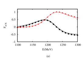
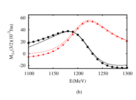
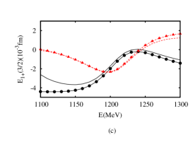
Figure 6: Energy dependence of the $\pi N$ amplitude(a) and the $\gamma\pi$ $M_{1+}(3/2)$(b) and $E_{1+}(3/2)$(c) amplitudes of $P_{33}$ channel. The solid circle(triangle) shows real(imaginary) part of the amplitude calculated using Eq. (15). The solid (dashed) curve shows real(imaginary) part of the amplitude of EBC-DCC model.

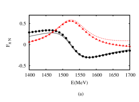
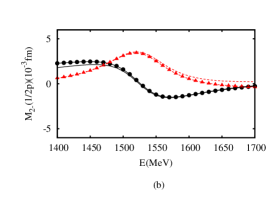
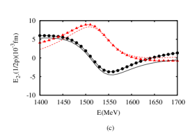
Figure 7: Energy dependence of the the $\pi N$ amplitude(a) and the $\gamma\pi$ $M_{2-}(1/2p)$(b) and $E_{2-}(1/2p)$(c) amplitudes of $D_{13}$ channel. The solid circle(triangle) shows real(imaginary) part of the amplitude calculated using Eq. (15). The solid (dashed) curve shows real(imaginary) part of the amplitude of EBC-DCC model.

We now note that the expression Eq.(40) looks similar to the commonly used amplitude with a Breit-Wigner parametrization

$$T^{BW}_{\pi N,\gamma N}(E) = B_{\pi N,\gamma^{*}N}(Q^{2};E)+\frac{\Gamma^{1/2}_{\pi N}(E)e^{i\phi^{BW}(E)}A^{BW}_{\lambda}(Q^{2},E)}{E-(W_{R}-i\frac{\Gamma_{tot}(E)}{2})}.$$ (43)

where $\Gamma_{tot}(E=W_{R})$ and $\Gamma_{\pi N}(E=W_{R})$ are called the total width and partial decay width for $\pi N$ channel, respectively, and $A^{BW}_{\lambda}(Q^{2},q,E)$ is assumed to be real numbers. The energy dependence of these widths as well as the phase factor $\phi^{BW}(E)$ are parts of the assumptions in those analysis, which of course will influence how the non-resonant amplitude $B_{\pi N,\gamma^{*}N}(Q^{2};E)$ is adjusted to fit the data.

Eqs.(40) and (43) have similar structure, but they have important differences. First Eq.(40) is evaluated at complex $M_{R}$ and hence the on-shell momentum $q^{on}$ and $p^{on}$ are also complex. On the other hand, all energy and momentum variables in Eq.(43) are real numbers defined by the physical energy $E$. The non-resonant amplitude $B_{\pi N,\gamma N}$ in Eq.(40) is obtained from a coupled-channel calculation, while $B_{\pi N,\gamma^{*}N}(Q^{2};E)$ in Eq.(43) is often calculated from tree-diagrams of phenomenological Lagrangian with unitarization using $\pi N$ amplitude. Thus it is difficult to see that the helicity amplitudes of $\gamma^{*}N\rightarrow N^{*}$ extracted from these two rather different approaches can be compared.

The two-pole structure of $P_{11}$ resonances near $\pi\Delta$ threshold poses a problem in interpreting our results for the $\gamma^{*}N\rightarrow N^{*}$ form factors $A_{\lambda}(Q^{2})$. We note that Eqs.(40) is valid for each of these two poles, but they are on different Riemann surfaces. Thus we need to find a parametrization which carries the sheet information in representing these two-pole contributions. Here we follow the approach of Refs. kato65 ; fujii1 ; fujii2 and a similar formula used in extracting meson resonancesmp87 ; bugg .

We first use Eq.(40) to write the $\pi N\rightarrow\pi N$ and $\gamma N\rightarrow\pi N$ scattering amplitudes on the $\pi\Delta$ physical($a=p$) and unphysical($a$=$u$) sheet as

$$T^{(a)}_{\beta,\alpha}(p^{on}_{\beta},p^{on}_{\alpha},E\rightarrow M^{(a)}_{R}) = -\frac{R^{(a)}_{\beta,\alpha}}{E-M^{(a)}_{R}}+B^{(a)}_{\beta,\alpha},$$ (44)

where $\alpha,\beta$ represent $\pi N$ or $\gamma N$ channels. All parameters $R^{(a)}_{\beta,\alpha},B_{\beta,\alpha}^{(a)}$ and $M_{R}^{(a)}$ are obtained numerically from the amplitude as described in the previous section. The above two amplitudes with $a=u,p$ can be combined by using the following unified representation

$$T_{\beta,\alpha}(p^{on}_{\beta},p^{on}_{\alpha},E\rightarrow M_{R}) = -\frac{R_{\beta,\alpha}+R^{1}_{\beta,\alpha}p_{\pi\Delta}}{E-M_{R}-\gamma p_{\pi\Delta}}+B_{\beta,\alpha}+B^{1}_{\beta,\alpha}p_{\pi\Delta},$$ (45)

where $p_{\pi\Delta}$ is the $\pi\Delta$ on-shell momentum $p_{x}$ determined by Eq.(11). We require $T_{\beta,\alpha}=T_{\beta,\alpha}^{(p/u)}$ at $p_{\pi\Delta}=p_{\pi\Delta}^{(p/u)}$. This requirement for $\alpha=\pi N,\gamma N$ and $\beta=\pi N$ determines 6 unknown complex numbers $R,R^{1},M_{R},B,B^{1}$ and $\gamma$ from known parameters $R^{(a)}_{\beta,\alpha},B_{\beta,\alpha}^{(a)}$ and $M_{R}^{(a)}$. Neglecting small contribution of $R^{1}$ and $B^{1}$, we then obtain

$$T_{\beta,\alpha}(p^{on}_{\beta},p^{on}_{\alpha},E\rightarrow M_{R}) = -\frac{R_{\beta,\alpha}}{E-M_{R}-\gamma p_{\pi\Delta}}+B_{\beta,\alpha}$$ (46)

where

$$\gamma = \frac{M_{R}^{(p)}-M_{R}^{(u)}}{p_{\pi\Delta}^{(p)}-p_{\pi\Delta}^{(u)}}$$ (47)

$$M_{R} = M_{R}^{(p)}-\gamma p_{\pi\Delta}^{(p)}$$ (48)

$$R^{1}_{\beta,\alpha} = \frac{R_{\beta,\alpha}^{(p)}(1-\gamma dp_{\pi\Delta}^{(p)}/dE)-R_{\beta,\alpha}^{(u)}(1-\gamma dp_{\pi\Delta}^{(u)}/dE)}{p_{\pi\Delta}^{(p)}-p_{\pi\Delta}^{(u)}}$$ (49)

$$R_{\beta,\alpha} = R_{\beta,\alpha}^{(p)}(1-\gamma dp_{\pi\Delta}^{(p)}/dE)-p_{\pi\Delta}^{(p)}R^{1}_{\beta,\alpha}.$$ (50)

With $p^{(u)}_{\pi\Delta}=49-68i$ MeV, $M^{(u)}_{R}=(1359-76i)$ MeV and $p^{(p)}_{\pi\Delta}=-65+86i$ MeV, $M^{(p)}_{R}=(1357-76i)$ MeV, we have $M_{R}=(1364-105i)$MeV, $\gamma=-0.146+0.062i$ and $R_{\pi N,\pi N}=(-12-47i)$MeV. The quantities $R^{(u/p)}_{\pi N,\gamma N}$ at $Q^{2}$ can be obtained from $\bar{\Gamma}^{R}_{\pi N}\bar{\Gamma}^{R}_{\gamma N}$ of Eq.(40) and hence $R_{\pi N,\gamma N}$ can also be calculated from using Eqs.(47)-(50). By interpreting $R_{\pi N,\pi N}$ and $R_{\pi N,\gamma N}$ of Eq.(46) as the residues of a pole and using the procedures described above, we can then extract the electromagnetic helicity amplitudes $A_{\lambda}(Q^{2})$ and $S_{\lambda}(Q^{2})$.

We have found that the unified formula Eq. (46) is a good approximation for both $\pi N$ and $\gamma\pi$ amplitudes if Eq.(44) is evaluated in the physical region where $E$ is near $W_{R}=Re(M_{R})$. This is shown in Fig. 8 for the considered $P_{11}$ partial wave. Although Eq.(46) is close to the commonly used Breit-Wigner form of Eq.(43), it is difficult to compare the extracted $\gamma^{*}N\rightarrow N^{*}$ helicity amplitude $A_{\lambda}(Q^{2})$ with those from previous analysis using Breit-Wigner parametrization, for the same reasons discussed above for the isolated $P_{33}$ and $D_{13}$ resonances.

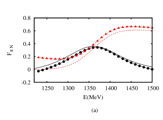
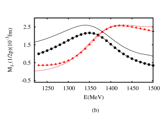
Figure 8: Energy dependence of the $P_{11}\pi N$ scattering(a) and the $M_{1-}(1/2p)$ $\gamma\pi$ amplitude(b). The solid circle(triangle) shows real(imaginary) part of the amplitude calculated using Eq. (46). The solid (dashed) curve shows real(imaginary) part of the amplitude of EBC-DCC model.

We now present in Table 4 our results for the $\gamma^{*}N\rightarrow N^{*}$ for the $P_{33}$, $D_{13}$ and $P_{11}$ resonances at $Q^{2}=0$ photon point. As comparisons, we also list several previous resultsarndt04 ; ahrens04 ; dugger07 ; blanpied01 which were extracted from using the Briet-Wigner parametrization of resonant amplitude. Our results are complex numbers, as expected from expression Eqs.(35)-(37). Here we mention that a recent nucleon resonance analysisbonn-catchina also yields complex helicity amplitudes.

We observe in Table 4 that the real parts of our results for $P_{33}$ and $D_{13}$ are in good agreement with the listed previous results. For the $P_{33}$ case, this good agreement is perhaps related to the fact that the imaginary parts of our results for this pronounced resonance is much smaller than their real parts. For $D_{13}$, a more detailed analysis is needed to understand this comparison since $D_{13}$ involves large $\pi N$ inelasticity and our results have large imaginary parts. For $P_{11}$ resonances, the real parts of our results (2c-bw) calculated from using the unified form Eq.(46) do not agree with the previous analysis using Breit-Wigner parametrization Eq.(43). This is perhaps also related to the fact that our results for each pole near $\pi\Delta$ threshold have large imaginary parts, as also seen in Table 4.

Table 4: The extracted $\gamma N\rightarrow N^{*}$ helicity amplitudes ($A_{\lambda}$ in $10^{-3}GeV^{-1/2}$) are compared with previous results.

		EBAC	Arndtarndt04	Ahrensahrens04	Duggerdugger07	Blanpiedblanpied01
$P_{33}(1210)$	$A_{3/2}$	-265+19i	$-243\pm 1$	$-256\pm 3$	$-258\pm 5$	$-266.9\pm 1.6\pm 7.8$
	$A_{1/2}$	-129+44i	$-129\pm 1$	$-137\pm 5$	$-139\pm 4$	$-135.7\pm 1.3\pm 3.7$
$D_{13}(1527)$	$A_{3/2}$	171+91i	$167\pm 5$	$147\pm 10$	$143\pm 2$
	$A_{1/2}$	-31+29i	$-20\pm 7$	$-38\pm 3$	$-28\pm 2$
$P11(2cbw)$	$A_{1/2}$	-28+20i	$-63\pm 5$		$-51\pm 2$
$\,\,\,\,\,\,\,\,(1356)$	$A_{1/2}$	-13+20i
$\,\,\,\,\,\,\,\,(1364)$	$A_{1/2}$	-14+22i

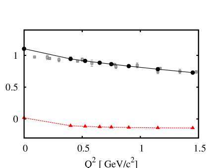
Figure 9: The magnetic $N$-$\Delta$ (1232) transition form factor $G^{*}_{M}(Q^{2})$ defined in Ref.sl96 . $F_{D}=1/(1+Q^{2}/b^{2})^{2}$ with $b^{2}=0.71$ (GeV/c)². The solid circles (solid triangles) are the real (imaginary) parts of our results. The other data points are from previous analysisndff-data .

For $P_{33}$ we can use the standard relationsl96 to evaluate the $N$-$\Delta$ magnetic transition form factor $G_{M}^{*}$ in terms of helicity amplitudes. The real parts of our results (solid circles connected by solid curve) in Fig.9 are in good agreement with the results (open circles with errors) from the previous analysismaid ; inna using Breit-Wigner parametrization. In the same figure, we also show that the imaginary parts (triangles connected by dotted line) of our results are much weaker. This observation further suggests that our results could be close to the results from analysis based on the Breit-Wigner parametrization only for the cases that the imaginary parts of our results are small.

For the $D_{13}(1527)$ resonance, our results are shown in Fig. 10. As an example in seeing the difficulty in comparing our results with those extracted from analysis using Breit-Wigner parametrization, we also show the the results (open circles with errors) from CLAS collaborationinna . Qualitatively, CLAS analysis is based on the Eq.(43) with the choice of $\phi^{BW}=0$. Thus their Breit-Wigner amplitude become pure imaginary at $E=W_{R}$ with $W_{R}$ taken from PDG. As discussed in the beginning of this section, i.e. expression Eq.(17), the phase factor $e^{i\phi(E)}$ is a necessary consequence of the presence of the non-resonance term $B_{\pi N,\gamma^{*}N}(p,Q^{2};E)$ under the unitarity condition. This difference between the CLAS analysis and the previous analysisdalitz ; taylor ; mcvoy should be noted in interpreting their extracted $\gamma^{*}N\rightarrow$ form factors.

Despite the differences between two different analysis, we observe that the real parts (solid circles connected by solid curve) of our $A_{3/2}$ and $A_{1/2}$ shown in Fig. 10 are qualitatively similar to the CLAS data. The imaginary parts (solid triangle connected by dashed curve) of our results, which are smaller than the real parts but still appreciable, are also shown there. Since the longitudinal parts of the amplitudes could not be well determined with the available data, the large differences between our results and the CLAS data seen in Fig. 10 are not very surprising.

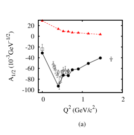
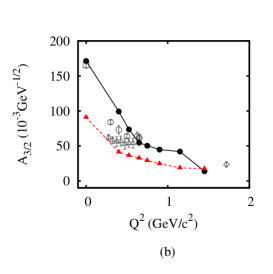
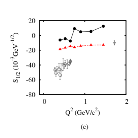
Figure 10: The extracted $\gamma N\rightarrow N^{*}(D_{13}(1527))$ form factors ($A_{1/2}$(a),$A_{3/2}$(b),$S_{1/2}$(c)). The solid circles(solid triangles) are their the real(imaginary) parts. The data are from CLAS collaborationinna .

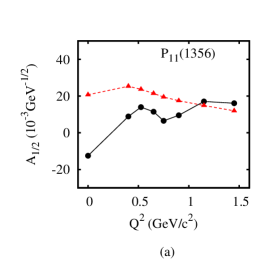
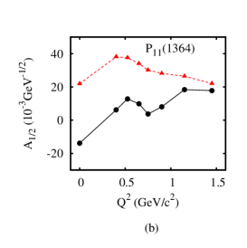
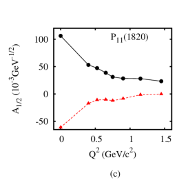
Figure 11: The extracted $\gamma N\rightarrow N^{*}(1356)$(a),$N^{*}(1364)$(b) and $N^{*}(1820)$(c) transition form factors. The solid circles (solid triangles) are their real (imaginary) parts.

Our results for the three poles of $P_{11}$ listed in Table I are shown in Fig. 11. Similar to the results at photon point presented in Table III, their imaginary parts (solid triangles) are comparable or larger than the real parts(solid circles) in magnitudes. We note that the momentum dependence of the helicity amplitudes indicates that the structure of $N^{*}(1356)$ and $N^{*}(1364)$ is quite different from $N^{*}(1820)$.

It is perhaps more appropriate to interpret our results calculated from using the unified form Eq.(44) for the two poles near the $\pi\Delta$ threshold as the values associated with the Roper $N^{*}(1440)$ resonance listed by PDG. This results are shown in Fig. 12. We again see that its imaginary parts (dotted line) are comparable or larger than real parts (solid line) in most of the $Q^{2}$ region. Here we also see that the contribution ( dot-dashed lines) from the determined bare $\gamma N\rightarrow N^{*}$ strengths play an important role in changing the sign of the real part at $Q^{2}\sim$ 0.4 (GeV/c)². This sign change of the bare $\gamma N\rightarrow N^{*}$ form factor is seen in some relativistic constituent quark model calculationscapstick ; inna-1 . This suggests that our bare parameters can perhaps be interpreted in terms of hadron structure calculations excluding the meson-baryon coupled-channel effects which is determined by unitarity condition. Here we mention that our real parts are qualitatively similar to the results from CLAS collaboration. But it is not clear how to make connection between two results since we have very appreciable imaginary parts.

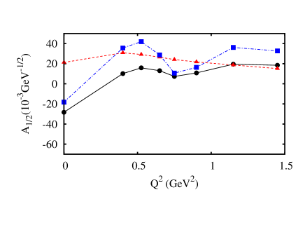
Figure 12: Helicity amplitude $A_{1/2p}$ of $P_{11}$ resonance at $\pi\Delta$ threshold extracted from using the unified representation Eq.(46). Solid (triangle) shows the real(imaginary) part of the helicity amplitude. Solid square (connected by dot-dashed line) shows contribution of the bare form factor.

V summary

We have explained the application of a recently developed analytic continuation method to extract the electromagnetic transition form factors for the nucleon resonances ($N^{*}$) within the EBAC-DCC model of meson-baryon reactions. We discuss in detail how the contours for solving the considered coupled-channels integral equations are chosen to find resonance poles $M_{R}$ and their residues. The formula for determining the $\gamma^{*}N\rightarrow N^{*}$ transition form factors $A_{\lambda}(Q^{2})$ and $S_{\lambda}(Q^{2})$, defined on the complex Riemann energy sheet, from the extracted residues are presented.

We have found that the resulting Laurent expansions of the $\pi N\rightarrow\pi N$ and $\gamma N\rightarrow\pi N$ amplitudes, evaluated in the physical energy region, can reproduce to a very large extent the exact solutions of EBAC-DCC model at energies near $E=Re(M_{R})$. A formula has been developed to give an unified representation of the effects due to the first two $P_{11}$ resonances, which are near the $\pi\Delta$ threshold, but are on different Riemann sheets. Illustrative results for the well isolated $P_{33}$ and $D_{13}$, and the complicated $P_{11}$ resonances are presented.

We discuss the differences between our results and those extracted from the approaches using the Breit-Wigner parametrization of resonant amplitude to fit the data. We find that there is no simple connection between these two different approaches, despite that some of the real parts of our results and the results from Breit-Wigner analysis agree qualitatively when the imaginary parts of our results are much smaller.

To conclude, we emphasize that our form factors are defined in a well-studied theoretical frameworkdalitz ; taylor ; mcvoy within which a resonance is an ”eigen state” of the Hamiltonian with the outgoing boundary condition for the asymptotic wavefunction of its decay channels. Thus the electromagnetic transition form factors defined by $<\psi^{R}_{N^{*}}|J_{em}|N>$ , which can be extracted from the residues of resonance poles, must be complex, since the resonant wavefunction $\psi^{R}_{N^{*}}$ contains scattering continuum. This must be accounted for in comparing our results with those from using the Breit-Wigner form to fit the data and any hadron structure calculations of $N$-$N^{*}$ transition form factors, such as those from relativistic quark modelscapstick ; inna-1 , Dyson-Schwinger modelsroberts , and LQCDlqcd .

- (1) N. Suzuki, T. Sato and T. -S. H, Lee, Phys. Rev. C79, 025205 (2009).
- (2) N. Suzuki, B. Julia-Diaz, H. Kamano, T.-S. H. Lee, A. Matsuyama, T. Sato, Phys. Rev. Lett. 104, 042302 (2010)
- (3) B. Julia-Diaz, T. -S. H. Lee, A. Matsuyama, and T. Sato, Phys. Rev. C76, 065201 (2007).
- (4) A. Matsuyama, T. Sato, and T. -S. H. Lee, Phys. Rept. 439, 193 (2007).
- (5) B. C. Pearce and I. R. Afnan, Phys. Rev. C 34, 991 (1986); 40, 220 (1989).
- (6) F. Gross and Y. Surya, Phys. Rev. C 47, 703 (1993).
- (7) T. Sato, T-.S. H. Lee, Phys. Rev. C54, 2660 (1996)
- (8) C. T. Hung, S. N. Yang, and T.-S. H. Lee, Phys. Rev. C 64, 034309 (2001).
- (9) A. M. Gasparyan, J. Haidenbauer, C. Hanhart, and J. Speth, Phys. Rev. C 68, 045207 (2003); M. Döring, C. Hanhart, F. Huang, S. Krewald, and U.-G. Meißner, Nucl. Phys. A829, 170 (2009).
- (10) B. Julia-Diaz, T. -S. H. Lee, A. Matsuyama, T. Sato and L. C. Smith, Phys. Rev. C77, 045205 (2008).
- (11) B. Julia-Diaz, H. Kamano, T. -S. H. Lee, A. Matsuyama, T. Sato and N. Suzuki, Phys. Rev. C80, 025207 (2009).
- (12) A. Bohm, Quantum mechanics: foundations and applications (Springer-Verlag, New York, 1993).
- (13) R. H. Dalitz and R. G. Moorhouse, Proc. Roy. Soc. Lond. A318, 279 (1970).
- (14) M. Döring, C. Hanhardt, F. Huang, S. Krewald and U.-G. Meißner, Phys.Lett. B681, 26 (2009)
- (15) R. A. Arndt, W. J. Briscoe, I. I. Strakovsky, and R. L. Workman, Phys. Rev C74, 45205 (2006).
- (16) D. Drechsel, S. S. Kamalov and L. Tiator, Eur. Phys. J. A 34, 69 (2007).
- (17) I.G. Aznauryan,V,D. Burkert, et al. (CLAS Collaboration), Phys. Rev. C80, 055203 (2009); V.I. Mokeev, V.D. Burkert, L. Elouadrhiri, G.V. Fedotov, E.N. Golovach, and B.S. Ishkhanov, Chin. Phys. C33, 1210 (2009).
- (18) R. J. Eden and J. R. Taylor, Phys. Rev. Lett. 11, 516 (1963).
- (19) D. Morgan and M.R. Pennington, Phys. Rev. Lett. 59, 2818 (1987).
- (20) J. Taylor, Scattering Theory (Wiley, New York, 1972).
- (21) K. W. McVoy, in Fundamentals in Nuclear Theory, edited by A. De-Shalit and C. Villi(IAEA, Vienna, 1967), p475.
- (22) L. A. Copley, G. Karl, and E. Obryk Nucl. Phys. B13, 303 (1969).
- (23) C. Amsler et al., Phys. Lett. B667, 1 (2008).
- (24) R.A. Arndt, J. M. Ford, L. D. Roper, Phys. Rev. D32, 1085 (1985).
- (25) R.E. Cutkosky and S. Wang, Phys. Rev. D. 42, 235 (1990); R. E. Cutkosky, C. P. Forsyth, R. E. Hendrick and R. L. Kelly, Phys. Rev. D20, 2839 (1979).
- (26) M. Kato, Ann. Phys. (N.Y.) 31, 130 (1965).
- (27) Y. Fujii and M. Kato, Phys. Rev. 188, 2319 (1969).
- (28) Y. Fujii and M. Fukugita, Nucl. Phys. B85, 179 (1975).
- (29) D. Bugg, J. Phys. G Nucl. Part. Phys. 37, 055002 (2010).
- (30) R. A. Arndt, W. J. Briscoe, I. I. Strakovsky, and R. L. Workman, Phys. Rev. C66, 055213 (2002); R. A. Arndt, I. I. Strakovsky, and R. L. Workman, Phys. Rev. C53, 430 (1996).
- (31) J. Ahrens et al., Eur. Phys. J. A21, 323 (2004); J. Ahrens et al., Phys. Rev. Lett, 88, 232002 (2002).
- (32) M. Dugger et al., Phys. Rev. C76, 025211 (2007).
- (33) G. Blanpied et al., Phys. Rev. C64, 025203 (2001).
- (34) A.V. Anisovich, E. Klempt,V.A. Nikonov, M.A. Matveev, A.V. Sarantsev, and U. Thoma, Eur. Phys. J. A44, 203 (2010).
- (35) W. Bartel et al.,Phys. Lett 28B, 148 (1968); K. Bätzner et al., Phys. Lett. 39B, 575 (1972); J. C. Alder et al., Nucl. Phys. B46, 573 (1972); S. Sterin et al., Phys. Rev. D12, 1884 (1975).
- (36) S. Capstick and B.D. Keister, Phys. Rev. D51, 3598 (1995)
- (37) I.G. Aznauryan, Phys. Rev. C76, 025212 (2007)
- (38) See the review by P. Maris and C.D. Roberts, Int.J.Mod.Phys. E12 297(2003).
- (39) H-W. Lin et al., Phys. Rev. D79, 034502 (2009).