Exact epidemic dynamics for generally clustered, complex networks

Abstract

The last few years have seen remarkably fast progress in the understanding of statistics and epidemic dynamics of various clustered networks. This paper considers a class of networks based around a concept (the locale) that allows asymptotically exact results to be derived for epidemic dynamics. While there is no restriction on the motifs that can be found in such graphs, each node must be uniquely assigned to a generally clustered subgraph to obtain analytic traction.

1 Introduction

Recent progress on analytic approaches to epidemics on clustered networks has been extremely fast. Models have been proposed based on households [25, 5, 6], and the more general concept of local-global networks [3, 4]. Another recent innovation has come from generalisations of random graph theory [20, 17, 12, 13, 15, 7], and at the same time, general methods have been proposed for manipulation of master equations [24, 23]. These complement the traditional epidemiological approach to clustering based on moment closure [16] that has recently been applied to graphs with more general motif structure [14].

This paper draws on much of this recent activity, making three main contributions. Firstly, a set of networks is defined using the concept of a locale (which is distinct from the recently introduced concept of a role [15] but closely related to the hypergraphs of [7]) that have no restriction on the motifs that can be present. Secondly, epidemic dynamics are derived for these networks—the first time that manifestly asymptotically exact results for transient epidemic dynamics of an large clustered network with non-homogeneous mixing outside the clusters have been derived. Finally, techniques are presented for practical efficient calculation of quantities of interest.

2 General Theory

2.1 Network generation

We start with the definition of a network (or graph—we use the terms interchangeably) $G$ of size $N$ as a set of nodes (vertices) $V$, and a set of links (edges) $E\subseteq V\times V$. Using $\mathbb{Z}_{N}$ to stand for the set of integers from 1 to $N$, nodes are indexed by $i,j,\dots\in\mathbb{Z}_{N}$. The information contained in a network can be encoded in an adjacency matrix $\mathbf{A}=(A_{ij})$, whose elements are given by

$$A_{ij}=\begin{cases}1&\text{ if }\left(i,j\right)\in E\text{ ,}\\ 0&\text{ otherwise.}\end{cases}$$ (1)

Here we consider symmetric, non-weighted networks without self-links and so $A_{ii}=0$, $A_{ij}=A_{ji}$.

We now present a model for network creation that has been essentially considered in the context of random graph theory [7]. This starts by defining a set of objects we call here stubby subnets, which are indexed by type $\sigma$. A stubby subnet of type $\sigma$ and size $n_{\sigma}$ consists of three elements:

1. A set of nodes $v^{\sigma}\cong\mathbb{Z}_{n_{\sigma}}$;

2. A set of within-subnet links, $e^{\sigma}\subseteq v^{\sigma}\times v^{\sigma}$, with a within-subnet adjacency matrix $\mathbf{a}^{\sigma}$ defined as for $\mathbf{A}$ above;

3. A vector of ‘stubs’ $\mathbf{s}^{\sigma}$, such that $\forall i\in v^{\sigma},s_{i}^{\sigma}\in\mathbb{Z}_{+}$.

A full network is then constructed in the following way. We choose a finite number of stubby subnet types, indexed by $\sigma$, and pick a number $N_{\sigma}\gg 1$ of each stubby subnet type. Using tensor sums $\oplus$ to represent the aggregation of objects without the removal of ‘duplicates’ that would be implicit in set-theoretic union, the network size, nodes and first part of the link set are given respectively by

$$N=\sum_{\sigma}N_{\sigma}n_{\sigma}\text{ ,}\qquad V=\bigoplus_{\sigma}\bigoplus_{m=1}^{N_{\sigma}}v^{\sigma}\text{ ,}\qquad E_{1}=\bigoplus_{\sigma}\bigoplus_{m=1}^{N_{\sigma}}e^{\sigma}\text{ .}$$ (2)

The remainder of links are then provided by constructing a full vector of ‘stubs’ and connecting these using the standard Configuration Model [18] where distinct stubs are uniformly paired at random to form links.

$$\mathbf{S}=\bigoplus_{\sigma}\bigoplus_{m=1}^{N_{\sigma}}\mathbf{s}^{\sigma}\text{ ,}\quad E_{2}=\mathrm{ConfigurationModel}(V,\mathbf{S})\text{ ,}\quad E=E_{1}\cup E_{2}\text{ .}$$ (3)

In the limit where the network size $N$ is large, the duplicate links and self-edges produced through this construction should be Poisson distributed and independent of $N$ as in e.g. [11, Theorem 3.1.2] however for explicit generation of finite-size networks, the simple removal of duplicates implicit in (3) is commonly used and should not significantly alter the epidemic dynamics.

Having defined such a network, it is straightforward to calculate degree distributions and clustering coefficients, since a node $i$ from a stubby subnet of type $\sigma$ has degree and clustering coefficient

$$d_{i}=\sum_{j}A_{ij}=s_{i}^{\sigma}+\sum_{j}a_{ij}^{\sigma}\text{ , and}\quad\phi_{i}=\frac{\sum_{j,k}A_{ij}A_{ik}A_{jk}}{\sum_{j,k}A_{ij}A_{ik}(1-\delta_{jk})}=\frac{{(\mathbf{a}^{\sigma})^{3}}_{ii}}{d_{i}(d_{i}-1)}\text{ ,}$$ (4)

respectively. From consideration of the standard configuration model [11, 18], if all stubby subnets are internally connected then a giant component emerges provided

$$\sum_{\sigma}M_{\sigma}D^{\sigma}(D^{\sigma}-2)>0\text{ ,}\quad\text{where}\quad D^{\sigma}:=\sum_{i=1}^{n_{\sigma}}s_{i}^{\sigma}\text{ ,}\quad M_{\sigma}=\frac{N_{\sigma}}{\sum_{\sigma^{\prime}}N_{\sigma^{\prime}}}\text{ .}$$ (5)

2.2 Invasion and final size

We now introduce a framework for the determination of whether a network of the kind considered can support the invasion of a species obeying susceptible-infectious-recovered (SIR) dynamics. To do this, we define the concept of a locale, which is a stubby subnet of type $\sigma$, together with an ‘origin’ node $o\in v^{\sigma}$. Clearly, there are at least $\sum_{\sigma}n_{\sigma}$ such locales to consider, although symmetries may reduce the effective number of these. Locale types are denoted using indices like $\lambda=\left(\sigma,o\right)$.

Invasibility of a network of the type under consideration (i.e. one constructed from stubby subnets) can therefore be considered by constructing a branching process on locales. If we define a ‘locale next generation’ matrix as the number of secondary locales infected by an initially infected locale early in the epidemic, then we can use the dominant eigenvalue of such a matrix to define a threshold parameter.

In order to do this, we need to define two dynamical quantities. The first of these is $T$, the probability that infection eventually passes across a network link where one node starts infectious and the other susceptible. The second is $P_{\sigma}(j|o)$, which is the probability that within the locale $\left(\sigma,o\right)$, where infection is first introduced to node $o$, that infection eventually reaches node $j\in v^{\sigma}$. The calculation of these two quantities depends on the precise dynamical system underneath the transmission process, but once they have been determined, the locale next generation matrix (interpreted as the expected number of locales of type $\bar{\lambda}=\left(\bar{\sigma},\bar{o}\right)$ created by a locale of type $\lambda=\left(\sigma,o\right)$ early in the epidemic) is given by

$$\mathcal{K}^{L}_{\bar{\lambda}\lambda}=T\frac{M_{\bar{\sigma}}s^{\bar{\sigma}}_{\bar{o}}}{s_{\mathrm{tot}}}\left(\left(s_{o}^{\sigma}-1\right)+\sum_{j\in v_{\sigma}\ominus o}P_{\sigma}(j|o)s_{j}^{\sigma}\right)\text{ ,}$$ (6)

where the normalised total number of stubs in the network is

$$s_{\mathrm{tot}}=\sum_{\sigma}M_{\sigma}\sum_{i\in v_{\sigma}}s_{i}^{\sigma}\text{ .}$$ (7)

The expression (6) is essentially composed of three parts. Before the bracket is the relative weighting by stubs of susceptible locales of type $\bar{\lambda}$; within the bracket is firstly the number of stubs in the origin node of locales of type $\lambda$, subtracting 1 to allow for the link that passed infection to the origin node; and secondly within the bracket is the number of stubs attached to other nodes in locales of type $\lambda$ weighted by the probability that those nodes are locally infected by $o$. The locale basic reproduction number, which is different from the standard basic reproductive number $R_{0}$, is then the dominant eigenvalue of this matrix

$$R_{L}:=\left|\left|\mathcal{K}^{L}\right|\right|\text{ .}$$ (8)

By using a ‘susceptibility sets’ argument as in [5, 6], the final size of an epidemic can also be calculated using the following set of transcendental equations:

$$R_{\infty} =1-\frac{\sum_{\sigma}M_{\sigma}\sum_{i\in v_{\sigma}}x_{i}^{\sigma}}{\sum_{\sigma}M_{\sigma}n_{\sigma}}\text{ ,}$$ (9)

$$x_{i}^{\sigma} =1-P(i|\boldsymbol{\pi}^{\sigma})\text{ ,}$$

$$(\boldsymbol{\pi}^{\sigma})_{i} =\left((1-T)+T\sum_{\lambda^{\prime}}\frac{M_{\sigma^{\prime}}s_{o^{\prime}}^{\sigma^{\prime}}}{s_{\mathrm{tot}}}\tilde{x}_{o^{\prime}}^{\sigma^{\prime}}\right)^{s_{i}^{\sigma}}\text{ ,}$$

$$\tilde{x}_{i}^{\sigma} =1-P(i|\tilde{\boldsymbol{\pi}}^{\sigma,i})\text{ ,}$$

$$(\tilde{\boldsymbol{\pi}}^{\sigma,i})_{j} =\left((1-T)+T\sum_{\lambda^{\prime}}\frac{M_{\sigma^{\prime}}s_{o^{\prime}}^{\sigma^{\prime}}}{s_{\mathrm{tot}}}\tilde{x}_{o^{\prime}}^{\sigma^{\prime}}\right)^{s_{j}^{\sigma}-\delta_{i,j}}\text{ .}$$

Here $R_{\infty}$ is the proportion of the population that is ultimately infected by the epidemic, while $x_{i}^{\sigma}$ is the probability that the $i$-th node in a stubby subnet $\sigma$ avoids infection during the epidemic. The $j$-th element of vector $\boldsymbol{\pi}^{\sigma}$ is the probability that the $j$-th node in a stubby subnet $\sigma$ avoids global infection (i.e. through one of its stubs) during the epidemic, with $P(i|\boldsymbol{\pi}^{\sigma})$ standing for the probability that a node $i$ in $\sigma$ is ultimately infected given such a vector.

Each of the equations in (9) can be paraphrased in English: the first follows essentially from the definitions of the quantities involved, and states that the final epidemic size is one minus the proportion of nodes that avoid infection; the second states that nodes avoiding infection are neither infected locally nor globally; the third states that each global neighbour of a node that avoids infection either does not transmit along the relevant link, or avoids infection itself; the fourth states that contacts avoiding infection are not infected locally, and are not infected globally once the link to the original node is discounted; and the fifth states that contacts of contacts avoiding infection either do not transmit along the relevant links, or avoid infection themselves.

2.3 Full Dynamics

In order to consider full transient dynamics for the system, we assume that transmission of infection across a link is a one-step Poisson process, happening at rate $\tau$, and that recovery is Markovian with rate $\gamma$. Our methodology is straightforwardly extended to the case where transmission happens at a variable rate during an individual’s infectious period or the case of non-exponentially distributed recovery times through the addition of extra disease compartments; the density of phase-type distributions means that an arbitrarily good approximation can be made given a sufficiently large state space [19]. It is also possible to calculate invasion thresholds and final sizes for arbitrary recovery times (i.e. without approximation by a phase-type distribution) since these rely only on the probability of transmission across a global link, $T$ (which is $\tau/(\tau+\gamma)$ in the Markovian case) and ‘multitype’ final sizes that can also be calculated in generality [2].

2.3.1 Notation

Since the full model dynamics we consider are rather hard to write down, we make use of Dirac ‘bra-c-ket’ formalism, using the appropriate links to Markov chains [10], to allow sufficiently compact notation for the full dynamical system. While this notation may not be familiar to mathematicians without experience of theoretical physics, it has been used in expository accounts of e.g. vector spaces [8].

Let $\mathcal{V}$ be a vector space, with elements $\left|\right>\in\mathcal{V}$ (called kets). The inner product (or bracket) is a map

$$\mathcal{V}\times\mathcal{V}\rightarrow\mathbb{R}\text{ ,}\qquad(\left|x\right>,\left|y\right>)\mapsto\left<x|y\right>\text{ .}$$ (10)

A bijection exists between $\mathcal{V}$ and its adjoint vector space $\mathcal{V}^{*}$, which has elements $\left<\right|\in\mathcal{V}^{*}$ (called bras). This bijection maps $\left|x\right>\in\mathcal{V}$ to $\left<x\right|\in\mathcal{V}^{*}$, $\forall x$, meaning that the inner product can be used to define a product

$$\mathcal{V}^{*}\times\mathcal{V}\rightarrow\mathbb{R}\text{ ,}\qquad(\left<x\right|,\left|y\right>)\mapsto\left<x\right|\cdot\left|y\right>:=\left<x|y\right>\text{ .}$$ (11)

Since the distinction between this product and the inner product does not matter for performing calculations, all objects of the form $\left<|\right>$ are often simply called ‘brackets’.

Operators, written in the form $\hat{\mathcal{O}}$, are maps

$$\hat{\mathcal{O}}:\mathcal{V}\rightarrow\mathcal{V}\text{ .}$$ (12)

Where $\mathcal{V}$ is spanned by a set of basis vectors, such operators can be defined uniquely through their action on each of this set’s elements. A special class of operators are projections, written in the form $\left|\right>\left<\right|$, which are defined to obey

$$\left|y\right>\left<y\right|:\mathcal{V}\rightarrow\mathcal{V}\text{ ,}\qquad\left|y\right>\left<y\right|\left|x\right>\mapsto\left<y|x\right>\left|y\right>\text{ .}$$ (13)

The final, general notational convention to introduce is tensor multiplication of vectors and operators. Where $\left|x\right>\in\mathcal{V}$, $\left|\tilde{x}\right>\in\tilde{\mathcal{V}}$, and $\hat{\mathcal{O}}_{1}:\mathcal{V}\rightarrow\mathcal{V}$, $\hat{\mathcal{O}}_{2}:\tilde{\mathcal{V}}\rightarrow\tilde{\mathcal{V}}$,

$$\left|x\right>\otimes\left|\tilde{x}\right>\in\mathcal{V}\times\tilde{\mathcal{V}}\text{ ,}\qquad(\hat{\mathcal{O}}_{1}\otimes\hat{\mathcal{O}}_{2})(\left|x\right>\otimes\left|\tilde{x}\right>)=(\hat{\mathcal{O}}_{1}\left|x\right>)\otimes(\hat{\mathcal{O}}_{2}\otimes\left|\tilde{x}\right>)\text{ .}$$ (14)

Similarly, if $\left<y\right|\in\mathcal{V}^{*}$, $\left<\tilde{y}\right|\in\tilde{\mathcal{V}}^{*}$ then

$$\left<y\right|\otimes\left<\tilde{y}\right|\in\mathcal{V}^{*}\times\tilde{\mathcal{V}}^{*}\text{ ,}\qquad(\left<y\right|\otimes\left<\tilde{y}\right|)(\left|x\right>\otimes\left|\tilde{x}\right>)=\left<y|x\right>\left<\tilde{y}|\tilde{x}\right>\text{ .}$$ (15)

Tensor multiplication is associative and distributive over addition, and $\left|\right>^{\otimes n}$ denotes $n$ identical vectors tensor multiplied by each other.

To see how this notation works when applied to stochastic models, consider a Poisson process. For simple Markov chains like this, it is common to write the transition rates explicitly, after stating that the system is characterised by an integer-valued stochastic variable $N$:

$$N\rightarrow N+1\text{ at rate }\lambda\text{ .}$$ (16)

The limitation of expressions of the form (16) is that for more complex processes, a very long list of events and rates can be generated, making further manipulations difficult. The Kolmogorov equations for the Markov chain are an alternative definition:

$$\frac{d\mathbf{p}}{dt}=\mathbf{p}\mathbf{Q}\text{ , where}\quad\mathbf{p}=\left(\begin{array}[]{c}\text{Pr}(N=0)\\ \text{Pr}(N=1)\\ \text{Pr}(N=2)\\ \vdots\end{array}\right)\text{ ,}\quad\mathbf{Q}=\lambda\left(\begin{array}[]{cccc}-1&1&0&\cdots\\ 0&-1&1&\cdots\\ 0&0&-1&\cdots\\ \vdots&\vdots&\vdots&\end{array}\right)\text{ .}$$ (17)

Again, for complex stochastic processes this can quickly yield objects that are almost impossible to manipulate. To use Dirac notation, we first define a state-space and operator

$$\mathcal{S}=\text{span}\left\{\left|N\right>\right\}_{N=0}^{\infty}\text{ ,}\quad\hat{q}\left|N\right>=\left|N+1\right>\text{ .}$$ (18)

Having made these definitions, definition of the Markov chain can then be done extremely parsimoniously:

$$\frac{d}{dp}\left|p\right>=\hat{Q}\left|p\right>\text{ , where}\quad\hat{Q}=\lambda\left(\hat{q}-\mathbb{1}\right)\text{ .}$$ (19)

Clearly, the extra effort to obtain such an expression is superfluous for a model as simple as the Poisson process; however for the complex systems we consider later, alternatives are simply too unwieldy. Since probabilities must sum to one, we write

$$\left<1|p\right>=1\text{ ,}\quad\text{where}\quad\left|1\right>=\sum_{N=0}^{\infty}\left|N\right>\text{ ,}\quad\text{and}\quad\left<M|N\right>=\delta_{M,N}\text{ .}$$ (20)

Here and throughout, $\delta$ is the Kronecker delta function. The normalising ‘ket’ $\left|1\right>$ is henceforth used to stand for an unweighted sum over basis states for the system under consideration.

2.3.2 Within-subnet dynamics

Here we consider stochastic epidemics dynamics for a network of size $n$ with adjacency matrix $\mathbf{a}$. Our starting point is a node-level state space

$$\mathcal{S}=\text{span}\left\{\left|S\right>,\left|I\right>,\left|R\right>\right\}\text{ ,}$$ (21)

Defined such that, where we use letters $A,B,\ldots$ to represent generic disease states

$$\left<A|B\right>=\delta_{A,B}\text{ .}$$ (22)

We then define five abstract operators: three that return the appropriate infection state

$$\hat{S}\left|S\right> =\left|S\right>, \hat{S}\left|I\right> =0, \hat{S}\left|R\right> =0,$$

$$\hat{I}\left|S\right> =0, \hat{I}\left|I\right> =\left|I\right>, \hat{I}\left|R\right> =0,$$

$$\hat{R}\left|S\right> =0, \hat{R}\left|I\right> =0, \hat{R}\left|R\right> =\left|R\right>;$$ (23)

and two that correspond to transmission and recovery

$$\hat{t}\left|S\right> =\left|I\right>, \hat{t}\left|I\right> =0, \hat{t}\left|R\right> =0,$$

$$\hat{r}\left|S\right> =0, \hat{r}\left|I\right> =\left|R\right>, \hat{r}\left|R\right> =0.$$ (24)

So a general state under consideration obeys

$$\left|p\right>\in\mathcal{S}^{n}\text{ ,}\quad\left<1|p\right>=1\text{ , where }\left|1\right>:=\left(\left|S\right>+\left|I\right>+\left|R\right>\right)^{\otimes n}\text{ .}$$ (25)

Where $\hat{\mathcal{O}}$ is an operator defined to act on elements of $\mathcal{S}$, we define an operator acting on the complete state space using subscripting so that

$$\hat{\mathcal{O}}_{i}:=\mathbb{1}\otimes\cdots\underbrace{\otimes\hat{\mathcal{O}}\otimes}_{i\text{th place}}\cdots\mathbb{1}\text{ .}$$ (26)

Having set up this machinery, we can now write the system’s dynamics in an extremely compact form:

$$\frac{d}{dt}\left|p\right>=\hat{Q}\left|p\right>\text{ , where }\hat{Q}=\tau\sum_{i}(\hat{t}_{i}-\hat{S}_{i})\sum_{j}a_{ij}\hat{I}_{j}+\gamma\sum_{i}(\hat{r}_{i}-\hat{I}_{i})\text{ .}$$ (27)

Despite this compact expression, the actual dimensionality of the system above grows extremely quickly with network size for numerical and analytical work. Methods available for increasing the tractability of these equations, particularly for final outcomes, are discussed next.

Calculation of final outcomes

We are interested in calculation of the probability that a node $j$ experiences infection, given an initial probability vector

$$\left|\boldsymbol{\pi}\right>:=\sum_{\mu_{1}=0}^{1}\cdots\sum_{\mu_{n}=0}^{1}\prod_{j=1}^{n}\left((\boldsymbol{\pi})_{j}\hat{S}_{j}\right)^{1-\mu_{j}}\left((1-(\boldsymbol{\pi})_{j})\hat{I}_{j}\right)^{\mu_{j}}\left|1\right>\text{ .}$$ (28)

For the outcomes relevant to working out invasion thresholds like (6) the special case of exactly one initial infection is simply a special case:

$$\left|o\right>:=\hat{I}_{o}\prod_{j\neq o}\hat{S}_{j}\left|1\right>\text{ .}$$ (29)

An insight from Bailey [1] is that the probability that a node $j$ recovers increases at a rate $\gamma$ multiplied by the probability that it is currently infectious. This means that if (27) holds, for initial condition (28), then

$$P(j|o)=\int_{0}^{\infty}\gamma\left<I_{j}\right|e^{\hat{Q}t}\left|\boldsymbol{\pi}\right>dt\text{ , where}\quad\left|{I}_{j}\right>:=\hat{I}_{j}\left|1\right>\text{ ,}$$ (30)

where exponentiation of an operator is defined through the power series

$$e^{\hat{\mathcal{O}}}=\mathbb{1}+\sum_{k=1}^{\infty}\frac{\hat{\mathcal{O}}^{k}}{k!}\text{ .}$$ (31)

In order to evaluate (30) efficiently, we can make use of the general theory of path integrals for Markov chains [22]. Since the presence of absorbing states in (30) would cause the integral to be poorly defined, we need first to decompose the state space into an absorbing set $\mathcal{A}$ and a non-absorbing set $\mathcal{C}$:

$$\mathcal{S}^{n}=\mathcal{A}\cup\mathcal{C}\text{ ,}$$ (32)

which can be done through the definition of projection operators

$$\hat{P}_{\mathcal{A}}=\sum_{\{A_{i}\}_{i=1}^{n}\in\{S,R\}^{\otimes n}}\left|A_{1}\right>\otimes\cdots\otimes\left|A_{n}\right>\left<A_{1}\right|\otimes\cdots\otimes\left<A_{n}\right|\text{ ,}\quad\hat{P}_{\mathcal{C}}=\mathbb{1}-\hat{P}_{\mathcal{A}}\text{ .}$$ (33)

The quantities of interest can then be written

$$P(j|\boldsymbol{\pi})=\left<\boldsymbol{\pi}|z\right>\text{ ,}$$ (34)

where

$$\bigg{(}\tau\sum_{i}(\hat{t}_{i}^{\dagger}-\hat{S}_{i})\sum_{j}a_{ij}\hat{I}_{j}+\gamma\sum_{i}(\hat{r}_{i}^{\dagger}-\hat{I}_{i})\bigg{)}\hat{P}_{\mathcal{C}}\left|z\right>=-\gamma\left|I_{j}\right>\text{ ,}$$ (35)

an equation that uses new operators

$$\hat{t}^{\dagger}\left|S\right> =0, \hat{t}^{\dagger}\left|I\right> =\left|S\right>, \hat{t}^{\dagger}\left|R\right> =0,$$

$$\hat{r}^{\dagger}\left|S\right> =0, \hat{r}^{\dagger}\left|I\right> =0, \hat{r}^{\dagger}\left|R\right> =\left|I\right>.$$ (36)

The final outcome probabilities can therefore be calculated through the solution of the set of linear equations (35).

An alternative is to use the ‘multi-type’ formula from Ball [2]. This approach has the disadvantage that a set of linear equations must be solved for each possible initial condition of the form (29), but the advantage of being able to include arbitrary distributions of recovery times. Supposing the probability density function for recovery time is $f(t)$, let

$$\Psi(s):=\frac{1}{\int_{0}^{\infty}e^{-st}f(t)dt}\text{ ,}$$ (37)

which obeys $\Psi(0)=1$ in general. Then for initial probability vector $\left|o\right>$, and final probability vector $\left|p^{\infty}_{o}\right>\in\mathcal{A}$, the following equation holds for any $\left|B_{1}\right>\otimes\cdots\otimes\left|B_{n}\right>\in\mathcal{A}$ :

$$\sum_{A_{1}\in\{S,B_{1}\}}\cdots\sum_{A_{o}=R}\cdots\sum_{A_{n}\in\{S,B_{n}\}}\left<A_{1}\right|\otimes\cdots\otimes\left<A_{n}|p^{\infty}_{o}\right>\prod_{i}\Psi\bigg{(}\tau\left<R_{i}|A_{i}\right>\sum_{j}a_{ij}\left<S_{j}|B_{j}\right>\bigg{)}=1\text{ .}$$ (38)

For Markovian recovery at rate $\gamma$, we have $\Psi(s)=(s+\gamma)/\gamma$, which leads to terms that look much like those obtained during the solution of (35), and indeed Bailey [1] notes that equations of the form (38) can be derived from equations of the form (35) in the case of a complete graph.

Automorphism-driven lumping

Recently, the technique of automorphism-driven lumping has been applied to epidemic dynamics on networks [24] and percolation [15]. This approach reduces the complexity of network problems by making systematic use of discrete symmetries of the network. In particular, the automorphism group of a graph $G$ of size $n$ with adjacency matrix $\mathbf{a}$ is a subset of the permutation group: $\mathrm{Aut}(G)\subseteq\mathrm{S}_{n}$. The elements of the automorphism group leave the adjacency matrix invariant:

$$\mathbf{M}\in\mathrm{Aut}(G)\quad\Leftrightarrow\quad\mathbf{a}=\mathbf{M}\mathbf{a}\mathbf{M}^{\top}\text{ .}$$ (39)

The use of this insight to lump epidemic equations requires some care in the labelling of dynamical variables [24]. Using the notation above, we relabel a generic dynamical state of the system

$$\left|A_{1}\right>\otimes\cdots\otimes\left|A_{n}\right>\equiv\left|\{(A_{1},1),\ldots,(A_{n},n)\}\right>\text{ ,}$$ (40)

i.e. we go from an ordered set of states to an unordered set of pairs of states and node numbers. ‘Lumped’ basis states for the dynamical system (27) can then be defined according to the orbits of the automorphism group—this means that states like the above are lumped together into classes like

$$L(A_{1},\ldots,A_{n})=\{\ \{(A_{1},M(1)),\ldots,(A_{n},M(n))\}\ |\ \mathbf{M}\in\mathrm{Aut}(G)\ \}\text{ ,}$$ (41)

where $M(i)$ is the index of the non-zero component of the $i$-th row of the permutation matrix $\mathbf{M}$. The dynamical equivalence of these states can be seen by repeated substitution of $\mathbf{a}\rightarrow\mathbf{M}\mathbf{a}\mathbf{M}^{\top}$ into (27). Clearly, lumping classes must contain states that all have the same eigenvalues of $\hat{S}$ and $\hat{I}$; and in the limiting case of a fully connected graph such that $\mathrm{Aut}(G)=\mathrm{S}_{n}$, only these aggregate eigenvalues are required to describe the system [24].

2.3.3 Global dynamics

Recently, a set of dynamics was presented that are a manifestly asymptotically exact description of the mean behaviour of an SIR epidemic on a configuration-model network [4] (equivalent to a stubby subnet model where all subnets have one node). The idea behind this construction is that, once numbers of half-links are allocated in the configuration model, then the formation of full links is a Poisson process that can be compounded with the epidemic process. Individuals therefore start the epidemic with half links, and the network is constructed at the same time as the epidemic tree, reducing the number of half-links in the system over time.

We now write this construction in Dirac vector space notation, so that this approach may be readily combined with the within-subnet dynamics above to define global dynamics. Our starting point is a set of states that represent a number of ‘remaining half-links’

$$\mathcal{S}=\text{span}\left\{\left|l\right>\right\}_{l=0}^{k_{\mathrm{max}}}\text{ , such that }\left<l^{\prime}|l\right>=\delta_{l,l^{\prime}}\text{ ,}$$ (42)

where $k_{\mathrm{max}}$ is the maximum node degree (or more generally maximum number of stubs). We define two operators on such states: a link number operator, and a link-number lowering operator:

$$\hat{l}\left|l\right>=l\left|l\right>\text{ ,}\qquad\hat{l}^{-}\left|l\right>=\begin{cases}\left|l-1\right>&\text{ if }l\geq 1\text{ ,}\\ 0&\text{ otherwise.}\end{cases}$$ (43)

We now consider how remaining half-links interact with disease state. These are taken as a tensor product,

$$\left|A,l\right>=\left|A\right>\otimes\left|l\right>\text{ , so that }\left<B,l^{\prime}|A,l\right>=\delta_{A,B}\delta_{l,l^{\prime}}\text{ .}$$ (44)

By construction, however, recovered individuals lose all their half-links, so the state space for this system is

$$\mathcal{S}=\text{span}\left\{\left|S,l\right>,\left|I,l\right>,\left|R,0\right>\right\}_{l=0}^{k_{\mathrm{max}}}\text{ .}$$ (45)

We then define four operators on this space, which we present in terms of their non-trivial action

$$\hat{t}\left|S,l\right> :=\left(\hat{t}\left|S\right>\right)\otimes\left|l\right>=\left|I,l\right>\text{ ,}$$ (46)

$$\hat{b}\left|S,l\right> :=\left(\hat{t}\left|S\right>\right)\otimes\left(\hat{l}^{-}\left|l\right>\right)=\left|I,l-1\right>\text{ ,}$$

$$\hat{l}^{-}\left|A,l\right> :=\left|A\right>\otimes\left(\hat{l}^{-}\left|l\right>\right)=\left|A,l-1\right>\text{ ,}$$

$$\hat{r}\left|I,l\right> :=\left|R,0\right>\text{ .}$$

Three of these operators are simple uplifts, but the operator $\hat{b}$ for global infection is new. To define the dynamics of this system, we start with a general state

$$\left|p\right>=\sum_{l=0}^{k_{\text{max}}}\left(x_{l}(t)\left|S,l\right>+y_{l}(t)\left|I,l\right>\right)+z(t)\left|R,0\right>\text{ ,}$$ (47)

which obeys

$$\left<1|p\right>=1\text{ , for }\left|1\right>:=\sum_{l=0}^{k_{\text{max}}}\left(\left|S,l\right>+\left|I,l\right>\right)+\left|R,0\right>\text{ .}$$ (48)

There is also a non-linear term for the density of infection amongst free half-links that appears in the system,

$$\rho[p]:=\frac{\left<1\right|\hat{I}\hat{l}\left|p\right>}{\left<1\right|\hat{l}\left|p\right>}\text{ .}$$ (49)

Then a representation of the expected SIR dynamics on a configuration-model network is given by

$$\hat{Q}[p] :=\gamma\left(\hat{r}-\hat{I}\right)+\tau\left(\hat{l}^{-}-\mathbb{1}\right)\hat{l}\hat{I}+\rho[p]\left(\gamma+\tau\right)\left(\hat{l}^{-}-\mathbb{1}\right)\hat{l}+\rho[p]\tau\left(\hat{b}-\hat{S}\right)\hat{l}\text{ ,}$$ (50)

$$\frac{d}{dt}\left|p\right> =\hat{Q}[p]\left|p\right>\text{ .}$$

The significance of these dynamics is that they do not grow in dimension with network size; in fact, they are asymptotically exact in the large system-size limit, which is inaccessible through simulation or direct integration of (27).

2.3.4 Full system dynamics

For a network made up of stubby subnets, it is possible to a make the same construction as above, where global links are made along with the epidemic process. In this case, a general state can be written

$$\left|p\right>=\sum_{\sigma,A_{1},\ldots,A_{n_{\sigma}},l_{1},\ldots,l_{n_{\sigma}}}{{p_{\sigma}}^{A_{1}\ldots A_{n_{\sigma}}}}_{l_{1}\ldots l_{n_{\sigma}}}(t)\left|\sigma\right>\otimes\left|A_{1},l_{1}\right>\otimes\cdots\otimes\left|A_{n_{\sigma}},l_{n_{\sigma}}\right>\text{ ,}$$ (51)

where $\left<\bar{\sigma}|\sigma\right>=\delta_{\bar{\sigma},\sigma}$ as would be expected. Clearly, any attempt to write down differential equations for the tensor representation of this system, ${{p_{\sigma}}^{A_{1}\ldots A_{n}}}_{l_{1}\ldots l_{n}}(t)$, will involve extremely complex expressions. By contrast, using the formalism of Dirac notation and operators that we have developed above, we can write the dynamics for this system as

$$\hat{P}_{\sigma} :=\sum_{A_{1},\ldots,A_{n_{\sigma}},l_{1},\ldots,l_{n_{\sigma}}}\left|\sigma\right>\otimes\left|A_{1},l_{1}\right>\otimes\cdots\otimes\left|A_{n_{\sigma}},l_{n_{\sigma}}\right>\left<A_{n_{\sigma}},l_{n_{\sigma}}\right|\otimes\cdots\otimes\left<A_{1},l_{1}\right|\otimes\left<\sigma\right|$$ (52)

$$\rho[p] :=\frac{\left<1\right|\sum_{\sigma}\sum_{i=1}^{n_{\sigma}}\hat{I}_{i}\hat{l}_{i}\hat{P}_{\sigma}\left|p\right>}{\left<1\right|\sum_{\sigma}\sum_{i=1}^{n_{\sigma}}\hat{l}_{i}\hat{P}_{\sigma}\left|p\right>}\text{ ,}$$

$$\hat{Q}_{\sigma}[p] :=\gamma\sum_{i=1}^{n_{\sigma}}\left(\hat{r}_{i}-\hat{I}_{i}\right)+\tau\sum_{i=1}^{n_{\sigma}}\left(\hat{l}^{-}_{i}-\mathbb{1}\right)\hat{l}_{i}\hat{I}_{i}$$

$$\quad+\tau\sum_{i=1}^{n_{\sigma}}\left(\hat{t}_{i}-\hat{S}_{i}\right)\sum_{j=1}^{n_{\sigma}}a^{\sigma}_{ij}\hat{I}_{j}$$

$$\quad+\rho[p]\left(\gamma+\tau\right)\sum_{i=1}^{n_{\sigma}}\left(\hat{l}^{-}_{i}-\mathbb{1}\right)\hat{l}_{i}+\rho[p]\tau\sum_{i=1}^{n_{\sigma}}\left(\hat{b}_{i}-\hat{S}_{i}\right)\hat{l}_{i}\text{ ,}$$

$$\frac{d}{dt}\left|p\right> =\sum_{\sigma}\hat{Q}_{\sigma}[p]\hat{P}_{\sigma}\left|p\right>\text{ .}$$

These equations have the same significance as above: the asymptotically exact expected epidemic dynamics of a class of clustered dynamics can be calculated for the large system-size limit of a network.

3 Examples

We now turn to some examples of the methodology presented above to specific networks. Throughout this section we work in natural units such that the recovery rate $\gamma=1$.

3.1 Invasion and final size

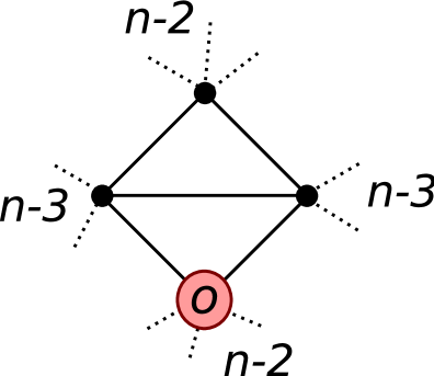
(a)

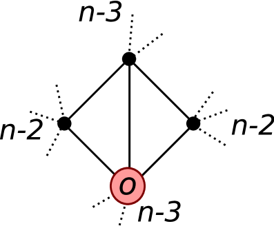
(b)

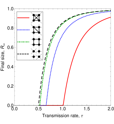
(c)

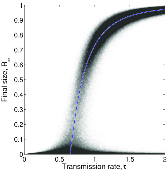
(d)

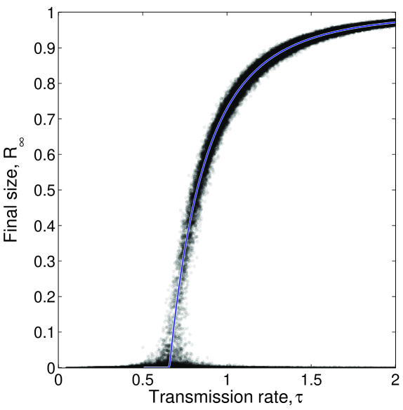
(e)

(f)

Figure 1: Epidemic final sizes on regular graphs with different generalised clustering. (a) and (b) show the two locales involved in general ‘envelope’-based graphs. For $n=4$, $\gamma=1$, (c) shows asymptotic final sizes for four different graphs, while remaining plots illustrate the rate of convergence to the asymptotic result by showing final sizes for $M$ runs on envelope-based networks of size $N$ where (d) $M=10^{6},N=10^{3}$, (e) $M=10^{5},N=10^{4}$, (f) $M=10^{5},N=5\times{}10^{4}$. Each dot represents a realisation, and blue lines are asymptotic results.

We consider invasion on the two locales shown in Figure 1(a,b). These networks are constructed from the envelope / diamond motif as shown, so that every individual has exactly $n$ links. This means that all differences between this model and an $n$-regular random graph derive from the presence and structure of short loops in the network and not heterogeneity in node degree. The locale basic reproductive ratio is given (after straightforward but tedious manipulations probably best carried out using a computer algebra system) by:

$$R_{L}=\big{(}\tau\big{(}2(n-3)^{2}+(n(25n-142)+204)\tau+(n(133n-716)+982)\tau^{2}\\ +(n(377n-1948)+2570)\tau^{3}+(n(563n-2846)+3672)\tau^{4}\\ +2(n(193n-968)+1239)\tau^{5}+12(8(n-5)n+51)\tau^{6}\big{)}\big{)}\\ /\big{(}(2n-5)(1+\tau)^{4}(1+2\tau)^{2}(1+3\tau)\big{)}\text{ .}$$ (53)

It is also possible to compare this envelope-based network to other networks that are also $n$-regular, but have different generalised clustering. This comparison is shown for final sizes where $n=4$ in Plot (c) of Figure 1; as would be expected, networks with more short loops are harder for a disease to invade.

The question might also be asked as to how quickly epidemics simulated using Monte Carlo methods on finite networks converge to the asymptotic results, which is considered in Figure 1(d,e,f). These show that even for networks of a few thousand nodes, asymptotic results provide a useful guide to expected behaviour.

3.2 Full Dynamics

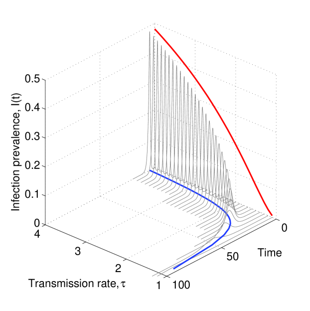
(c)

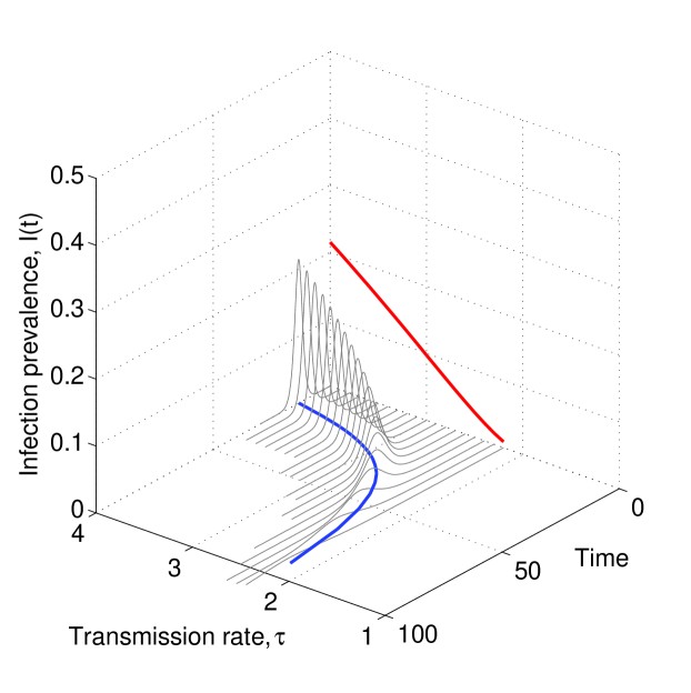
(d)

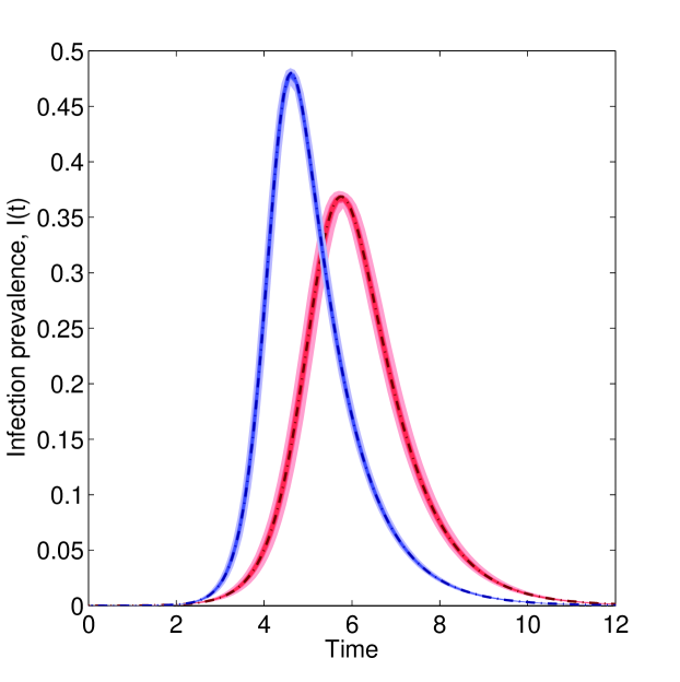
(e)

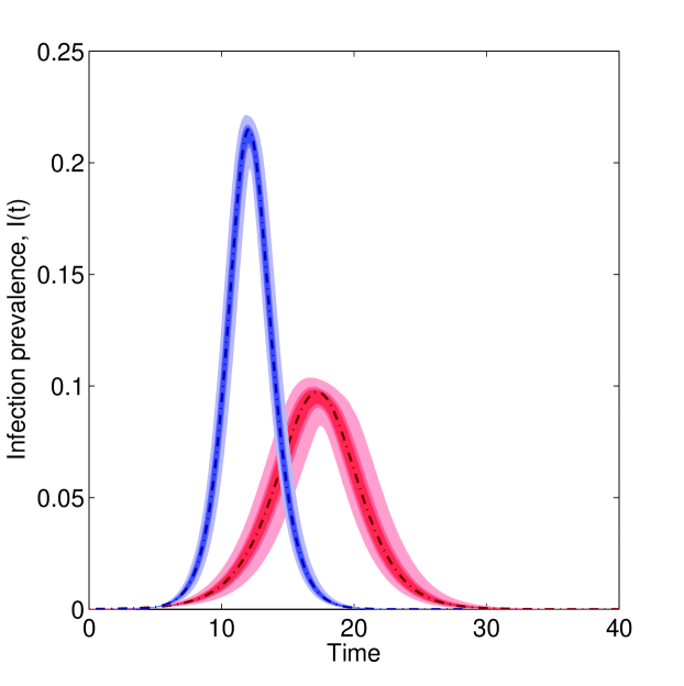
(f)

Figure 2: Exact transient epidemic dynamics for two special networks. (a) shows a typical location in the unclustered graph, and (b) shows a typical location in the clustered graph. Epidemic curves (grey) for different parameter values are shown in (c), (d) respectively. Peak times (blue) and peak heights (red) are projected onto the appropriate axes. (e) and (f) compare the asymptotic results (dot-dashed lines) to simulations on networks of size $N=10^{4}$ for $\tau=3$ (red) and $\tau=4$ (blue). Simulation prediction intervals at 50%, 67% and 95% are shown as shaded regions.

While invasion thresholds are of practical interest, transient dynamical features of epidemics are also important, and are not always simply determined by consideration of thresholds. Figure 2 shows the transient behaviour in the large system-size limit for two special graphs, both of which 3-regular: (a) a configuration-model network where each node has 3 stubs; (b) a stubby-subnet graph composed of triangles with each node having one stub. The dynamics as defined above give the epidemic curves shown in (c) for the CM network and (d) for the triangle-based network respectively. As above, we consider the relationship between these results and direct stochastic simulation, with results shown in (e) and (f). Clearly, convergence is fast for epidemics with a transmission rate much greater than the threshold, but near threshold stochastic, finite-size effects are much more significant.

4 Other solvable networks

It has been clear for some time that a network (or otherwise structured population) with a local-global distinction will admit a solution to an SIR epidemic on that network [3]. As a practical adjunct to this, both the local and global features of the network must individually admit solution. The stubby-subnet networks here propose one such distinction: each node can be uniquely assigned to a local unit of clustered structure; and global mixing happens through a configuration model network.

We now consider three other versions of this concept, firstly by introducing assortative mixing outside the subnet, secondly using the recently defined role-based networks, and finally to weighted networks.

4.1 Assortativity

In [21], a generalisation of the configuration model was developed to incorporate the notion of assortativity. Such assortativity (or even disassortativity) is a mainstay of epidemiology, and much theoretical effort has been expended to model its effects [9]. To describe assortativity, we introduce a correlation matrix ${C}_{\bar{\lambda},\lambda}$ (analogous to the $e_{kl}$ of [21]) that multiplies the probabilities that two locales are linked globally compared to the configuration model. For such a network, the locale next generation matrix is

$$\mathcal{K}^{L}_{\bar{\lambda}\lambda}=T\frac{M_{\bar{\sigma}}s^{\bar{\sigma}}_{\bar{o}}}{s_{\mathrm{tot}}}\left(\left(s_{o}-1\right)C_{\bar{\lambda},\lambda}+\sum_{j\in v_{\sigma}\ominus o}P_{\sigma}(j|o)s_{j}C_{\bar{\lambda},(\sigma,j)}\right)\text{ ,}$$ (54)

and an appropriate threshold parameter will be given by the dominant eigenvalue of this matrix. Exact transient dynamics for such a system should also be straightforward to write down: in addition to indexing a node with its effective remaining half-links and disease state, each node should also be indexed by locale. Instead of having homogeneous transmission on the basis of pairing half-links at rate $\tau$, the rate should then be multiplied by ${C}_{\bar{\lambda},\lambda}$. Of course, this yields equations that are at least quadratic rather than linear in maximum node degree, making numerical integration correspondingly more difficult.

4.2 Role-based networks

Role-based networks as considered in [20, 17, 15] involve a different definition of local and global. In these networks, it is links that can be uniquely assigned to a local unit of clustered structure, meaning that nodes can be attached to many different clustered subgraphs. This clearly allows a next-generation matrix to be established by indexing cases by the unit of structure through which they acquired infection, as in [17]. The definition of asymptotically exact dynamics is less clear in this case, however dynamical approaches such as [26] that are in extremely good numerical agreement with simulation, and may turn out to be large system-size limits through further work, can clearly be extended to role-based networks. The primary differences between stubby-subnet and role-based networks are that the former can specify an exact structure of stubs for each node in a clustered motif, while the latter can involve each node in several motifs. As such, these are best seen as complementary approaches to the fast-moving field of solvable clustered networks.

4.3 Weighted networks

While all networks discussed above have been topological (i.e. links are either present or not) all of the analysis above carries through exactly if within-subnet links are weighted, so that values $a^{\sigma}_{ij}\in\mathbb{R}_{+}$ can be substituted into e.g. (52). It is also possible to stratify global links into multiple contexts, each with a given strength (i.e. different values of $T$) although this latter modification does increase the system dimensionality, while weighting within-subnet dynamics does this only if the weighting breaks a discrete symmetry of the topological network.

5 Discussion

This paper has presented a manifestly asymptotically exact way to calculate transient epidemic dynamics on a class of clustered networks. As such, it complements existing work based on simpler network structure or moment closure; however, this is done at the cost of extremely high dimensional ODE systems, with even the simplest triangle-based example above involving 216 equations. Of course, computational resources continue to improve, and so the possibility of considering more complex networks and disease natural history cannot be ruled out, but is not currently easily done. At present, there is no perfect technique for the consideration of epidemic dynamics on networks: direct simulation is versatile, but hard to interpret; moment closure is numerically fast but the criteria under which it is accurate are currently unclear; and analytic approaches are either extremely high dimensional or restricted to special network types. In particular, local tree-like structure of some form has been a feature of all analytic approaches to date, and may be an indispensable assumption. This means that there is merit to development of all available approaches, and it is hoped that this paper broadens the range of networks on which certain epidemiological results can be computed, contributing to our understanding of the fast-moving but complex field of contact network epidemiology.

(a)

(b)

References

- [1] N. Bailey. The Mathematical Theory of Infectious Diseases and its Applications. Charles Griffin and Company, London, 1975.
- [2] F. Ball. A unified approach to the distribution of total size and total area under the trajectory of infectives in epidemic models. Advances in Applied Probability, 18(2):289–310, 1986.
- [3] F. Ball and P. Neal. A general model for stochastic SIR epidemics with two levels of mixing. Mathematical Biosciences, 180:73–102, Jan 2002.
- [4] F. Ball and P. Neal. Network epidemic models with two levels of mixing. Mathematical Biosciences, 212(1):69–87, Jan 2008.
- [5] F. Ball, D. Sirl, and P. Trapman. Threshold behaviour and final outcome of an epidemic on a random network with household structure. Advances in Applied Probability, 41(3):765–796, Jan 2009.
- [6] F. Ball, D. Sirl, and P. Trapman. Analysis of a stochastic SIR epidemic on a random network incorporating household structure. Mathematical Biosciences, 224(2):53–73, Apr 2010.
- [7] B. Bollobás, S. Janson, and O. Riordan. Sparse random graphs with clustering. Random Structures & Algorithms, 38(3):269–323, 2011.
- [8] P. Dennery and A. Krzymicki. Mathematics for Physicists. Harper and Row, 1967.
- [9] O. Diekmann and J. Heesterbeek. Mathematical Epidemiology of Infectious Diseases: Model Building, Analysis and Interpretation. J Wiley, 2000.
- [10] P. J. Dodd and N. M. Ferguson. A many-body field theory approach to stochastic models in population biology. PLoS ONE, 4(9):e6855, 09 2009.
- [11] R. Durrett. Random Graph Dynamics. Cambridge University Press, 2007.
- [12] J. P. Gleeson. Bond percolation on a class of clustered random networks. Physical Review E, 80(3):036107, Sep 2009.
- [13] J. P. Gleeson and S. Melnik. Analytical results for bond percolation and -core sizes on clustered networks. Physical Review E, 80(4):046121, Oct 2009.
- [14] T. House, G. Davies, L. Danon, and M. J. Keeling. A motif-based approach to network epidemics. Bulletin of Mathematical Biology, 71:1693–1706, Apr 2009.
- [15] B. Karrer and M. E. J. Newman. Random graphs containing arbitrary distributions of subgraphs. Physical Review E, 82(6):066118, Dec 2010.
- [16] M. J. Keeling. The effects of local spatial structure on epidemiological invasions. Proceedings of the Royal Society B, 266(1421):859–67, Apr 1999.
- [17] J. Miller. Percolation and epidemics in random clustered networks. Physical Review E, 80(2):020901, Aug 2009.
- [18] M. Molloy and B. Reed. A critical point for random graphs with a given degree sequence. Random Structures & Algorithms, 6(2/3):161–179, 1995.
- [19] M. F. Neuts. Probability distributions of phase type. In Liber amicorum Professor emeritus Dr. H. Florin, pages 173–206. Katholieke Universiteit Leuven, Departement Wiskunde, 1975.
- [20] M. Newman. Random graphs with clustering. Physical Review Letters, 103(5):1–4, Jul 2009.
- [21] M. E. J. Newman. Assortative mixing in networks. Physical Review Letters, 89(20):208701, Jan 2002.
- [22] P. K. Pollett and V. E. Stefanov. Path integrals for continuous-time Markov chains. Journal of Applied Probability, 39:901–904, 2002.
- [23] J. V. Ross, T. House, and M. J. Keeling. Calculation of disease dynamics in a population of households. PLoS ONE, 5:e9666, Jan 2010.
- [24] P. Simon, M. Taylor, and I. Kiss. Exact epidemic models on graphs using graph-automorphism driven lumping. Journal of Mathematical Biology, 62:479–508, 2011.
- [25] P. Trapman. On analytical approaches to epidemics on networks. Theoretical Population Biology, 71:160–173, March 2007.
- [26] E. M. Volz, J. C. Miller, A. Galvani, and L. Ancel Meyers. Effects of heterogeneous and clustered contact patterns on infectious disease dynamics. PLoS Computational Biology, 7(6):e1002042, June 2011.