Particle Acceleration and Magnetic Field Structure in PKS 2155-304: Optical Polarimetric Observations

Abstract

In this paper we present multiband optical polarimetric observations of the VHE blazar PKS 2155-304 made simultaneously with a H.E.S.S./Fermi high-energy campaign in 2008, when the source was found to be in a low state. The intense daily coverage of the dataset allowed us to study in detail the temporal evolution of the emission and we found that the particle acceleration timescales are decoupled from the changes in the polarimetric properties of the source. We present a model in which the optical polarimetric emission originates at the polarised mm-wave core and propose an explanation for the lack of correlation between the photometric and polarimetric fluxes. The optical emission is consistent with an inhomogeneous synchrotron source in which the large scale field is locally organised by a shock in which particle acceleration takes place. Finally, we use these optical polarimetric observations of PKS 2155-304 at a low state to propose an origin for the quiescent gamma-ray flux of the object, in an attempt to provide clues for the source of its recently established persistent TeV emission.

1 Introduction

Figure 1: R-band optical light-curve for PKS 2155-304 from 01 to 07 September 2008, showing the total flux variability (upper panel), fractional polarisation degree (middle panel) and EVPA rotation (lower panel). Each data point corresponds to an integration time of about 6 min. The flux points and polarisation degree are not corrected for the host galaxy contribution. Error bars are of the order of the size of the points.

Strong and variable linear polarisation is a defining property of BL Lacs, which unavoidably associates the observed emission with beamed synchrotron radiation from a relativistic jet viewed face-on. The polarimetric properties of these sources have been thoroughly studied at radio and optical wavelengths for over three decades, displaying rich phenomenology (e.g. Angel & Stockman 1980 and Saikia & Salter 1988). The inner jets of active galaxies present a morphology characterised by a stationary region of enhanced brightness, the “core”, and other luminous components (“knots”) moving at relativistic speeds and thought to be associated with the propagation of shock perturbations. These structures tend to be highly polarised in radio and are widely recognised as potential sites of particle acceleration and as responsible for the observed flux variability (Hughes et al., 1989). Core brightening and the appearance of new knots in the jet have been linked to flaring activity extending to gamma-ray energies (Jorstad et al., 2001).

These shocked regions are persistent and bright structures in the X-ray images of mis-aligned pc-scale jets, and have also been invoked to explain the quiescent level of emission observed from some blazars at these energies (e.g. Giebels et al. 2002). In blazars, these knots are not resolved due to the close alignment of the jet to the line of sight, but their existence is implied by analogy with similar objects, such as M 87 (Marshall et al., 2002). Despite the fact that in mis-aligned objects the knots are responsible for only a fraction of the flux emitted from the source, the geometrical alignment in blazars provides the required amount of Doppler boosting necessary to produce the low-level of continuous emission observed (Giebels et al., 2002).

Katarzyński et al. (2008) have recently modeled the full spectral energy distribution (SED) of PKS 2155-304 and identified the presence of such a background synchrotron component, which is associated with an extended jet component (presumably the integrated contribution from all X-ray-bright knots along the jet) capable of sustaining the low state X-ray flux observed from the source. At very-high energies (VHE), consistent detection of the BL Lac PKS 2155-304 by the H.E.S.S. telescopes has also established a low-level of $\gamma$-ray emission for this object which is stable over several years and strongly constrains the blazar’s VHE quiescent state (Aharonian et al., 2010), but whose origin is still unknown.

The low state of PKS 2155-304 ($z=0.116$) has been studied recently in a multiwavelength campaign by H.E.S.S. and the LAT instrument onboard Fermi (Aharonian et al., 2009), with which the observations presented here are simultaneous. The time-averaged SED of the source was modeled as a single-zone synchrotron-self Compton (SSC) process which fitted the entire profile. The derived relations between the optical and VHE fluxes suggest that the former provides the target photons for the inverse-Compton (IC) emission, but a detailed study of the energetics of the model shows that a single-zone description cannot accommodate the entire multiband temporal behaviour of the light-curve. Part of the aim of this paper is to exploit the contemporaneity of our data to propose an explanation for the lack of temporal correlation observed between the optical and the high-energy components of the SED, and to give further support to the proposal by Aharonian et al. (2009) that a multi-zone model is necessary to describe the quiescent state emission of this BL Lac.

PKS 2155-304 has been the target of several optical polarimetric campaigns which have probed its long and short term behaviour. The polarisation degree is observed to assume typical values between $\sim$ 3-7%, with significant variability registered down to sub-hour timescales (e.g. Andruchow et al. 2005). The polarisation vector shows evidence of a preferential direction within the range 100-140^∘ (Tommasi et al. (2001) and references therein). Frequency dependent polarisation (FDP) has also been detected on several occasions (Smith & Sitko, 1991; Smith et al., 1992; Allen et al., 1993) and determined to be intrinsic to the synchrotron source. In radio, the parsec-scale jet of PKS 2155-304 was imaged twice at 15 GHz by Piner & Edwards (2004) and Piner et al. (2008). A single jet component is resolved downstream from the radio core, moving with a derived bulk Lorentz factor $\Gamma\sim$ 3. Polarised radio flux was detected in those images coming from the core component alone, and the polarisation vector ($131^{\circ}$) was seen to be closely aligned with the jet-projected position angle (P.A. $\sim$ 140-160^∘). In the optically thin regime this is evidence for the presence of a dominant magnetic field component transverse to the flow. The polarisation degree of the core exhibited a spatial gradient between 3-8% that increased in the upstream direction.

The existence of a preferred position angle in optical similar to that of the mm-wave core favours the presence of a dominant or large scale component with a regular magnetic field which is associated with both emissions. Furthermore, similar values of the polarisation degree seen in both bands and the lack of polarised emission from other parts of the jet in the VLBI images suggests the unresolved polarised optical emission originates in the pc-scale radio core. This hypothesis will be adopted here, motivated as well by recent studies which used VLBI maps to compare the optical polarisation properties of the jet with the radio images, and associated the variable emission with the position of the 43 GHz core (Lister & Smith, 2000; Jorstad et al., 2007; Gabuzda et al., 2006).

2 Description of the Observations

The optical polarimetric campaign was conducted in early September 2008, between MJD 54710-54716. Observations were made with the 1.6 m Perkin-Elmer telescope at Pico dos Dias Observatory of the National Astrophysics Laboratory (OPD/LNA, Brazil), using the imaging polarimeter IAGPOL in linear polarisation mode. Multi-band images in the V, R and I filters were taken on all nights but the last of the campaign. The configuration of the polarimeter provides simultaneous measurements of the ordinary and extra-ordinary rays, allowing us to perform observations under non-ideal atmospheric conditions, since any atmospheric contributions will affect both rays equally; additionally, any sky contribution is expected to cancel out in the process. Photometric flux measurements are obtained simultaneously with the polarimetric ones. Standard polarisation stars from Smith et al. (1991) and Rector & Perlman (2003) were used for calibration. Single polarisation images were integrated from 8 $\times$ 45 s exposures, each at a different position of the polarimetric wheel. A precision of better than 1% in the polarisation degree was achieved. The temporal resolution of consecutive measurements in the R band was of the order of 8-10 min, whereas V and I images were taken at the beginning and end of each night to monitor the spectral evolution of the source. Data reduction was made with a specially developed analysis package for LNA polarimetric data, PCCDPACK (Pereyra, 2000).

3 Discussion of the Optical Polarimetric Data

Figure 2: Polarised versus total flux relation for the six nights of the campaign. The straight lines are fits to the data used to derive the polarisation properties of the variable component.

Table 1: Polarisation parameters of variable component.

MJD	$p_{\rm{var}}$	$\theta_{\rm{var}}$	$I_{\rm{var}}$
	(%)	(∘)	(mJy)
54711	$12.5\pm 1.3$	$84.9\pm 5.6$	$2.3\pm 0.6$
54712	$1.0\pm 0.6$	$70.0\pm 12.0$	$2.0\pm 0.2$
54713	$5.6\pm 1.4$	$102.2\pm 7.0$	$3.8\pm 0.6$
54714	$7.5\pm 1.4$	$120.1\pm 6.4$	$1.8\pm 0.8$
54715	$6.8\pm 1.3$	$123.6\pm 6.2$	$5.8\pm 0.8$
54716	$3.4\pm 1.9$	$125.4\pm 6.5$	$7.5\pm 1.0$

Figure 1 shows the R band light-curve for the total flux, polarisation fraction and electric vector position angle (EVPA) for all six nights of the optical campaign. The data presented in this figure (see also Table 2 at the end of the paper) represents the directly observed quantities, not corrected for the unpolarised contribution of the stellar continuum. For the remainder of the analysis, flux estimates as quoted in Dominici et al. (2006) were used to subtract the host galaxy contribution to the total emission.

The source was observed for three to six hours during each night with a minimum temporal resolution in the R band of $\sim$ 10 min, resulting in a week of well sampled intranight light-curves. The overall flux behaviour is qualitatively distinct from the changes in the polarisation properties of the emission, as noted before by Courvoisier et al. (1995) and Tommasi et al. (2001) for this same object. Flux variability is dominated by intranight activity, superimposed on a baseline level which increases towards the end of the campaign and is in agreement with the measurements from the ATOM telescope presented in Aharonian et al. (2009). A Lomb-Scargle power spectrum analysis (Scargle, 1982) reveals that the flux microvariability is describable as random fluctuations, with minimum variability timescales $<$ 1 hr, limited by the sampling of the lightcurve.

Although presenting some intranight activity, the temporal behaviour of the polarised flux was dominated by inter-night variations with larger relative amplitude than those of the unpolarised flux, varying by a factor of 3 during the campaign. The host-corrected polarisation degree varied smoothly between 3-11% along the six nights of observations, within the range typically registered for the source and similar to those seen for the radio core. A very similar “oscillatory” behaviour for the polarisation fraction can be seen in the optical lightcurves of Courvoisier et al. (1995), but the behaviour of the polarisation vector is very distinct at both epochs.

Visual inspection of the light-curves shows that the total photometric variability cannot be explained by variations in the polarised flux alone. Subtraction of the polarised flux from the photometric light-curves leave residual variability both in the intranight and the long-term flux variations. Conversely, dilution of a constant polarised component on a variable, unpolarised background cannot account for the observed behaviour of the polarisation degree, which changes in an uncorrelated fashion with respect to the total flux. Throughout our observations the EVPA underwent a quasi-linear counter-clockwise rotation of about $40^{\circ}$, at a rate of $\approx$ 7^∘ per day. The lack of correlation between the smooth, long-term evolution of the polarisation parameters and the flux behaviour is a common property of BL Lacs (Qian et al., 1991) in optical and must be explained.

3.1 Modelling of the Polarised Emission

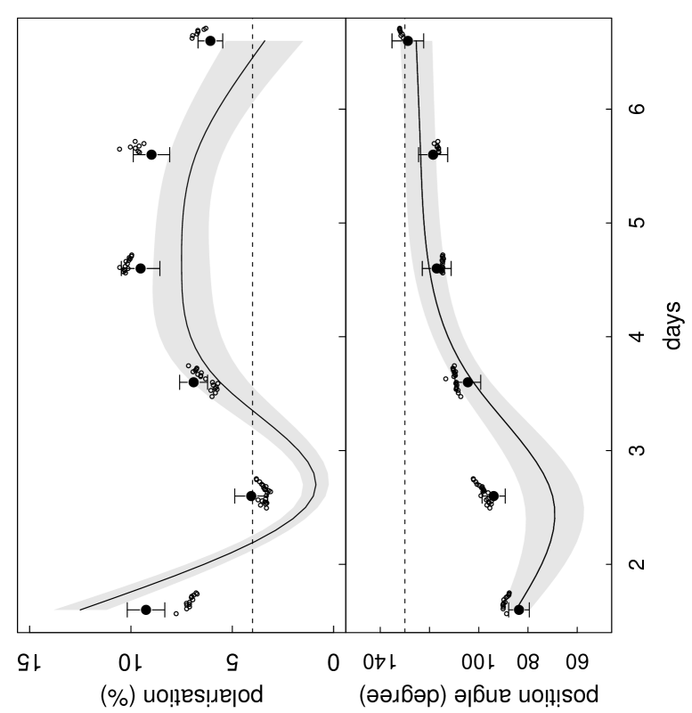
Figure 3: Results of the two-component synchrotron model fit to the optical polarimetric data of PKS 2155-304 (small dots). Large filled circles are the resulting model values for each night, obtained as the result of the superposition of a constant (dashed lines) and variable polarised component (smooth solid line) using the law of addition of polarised sources (Equations (1) and (2)). The smooth curves are a spline interpolation to the model values presented in Table 1 and show the temporal evolution of the variable component. Grey shades represent the confidence intervals as quoted in Table 1. The values for the constant component presented in the plots are $p_{\rm{cons}}=4\pm 1\%$ and $\theta_{\rm{var}}=130^{\circ}\pm 10^{\circ}$ for a ratio of fluxes $I_{\rm{var}}/I_{\rm{cons}}<1$. Notice in the bottom plot the rotation of the position angle of the model variable component towards a gradual alignment with the direction of the constant component.

If the observed variability within a given time interval is due to a single variable component with constant polarisation properties, a linear relationship exists between the absolute Stokes parameters Q and U and the total flux, as described in Hagen-Thorn et al. (2008). Figure 2 shows that although this relation is not obeyed by the entire dataset collectively, intranight measurements taken individually clearly follow a linear trend. This suggests that the flux microvariability could be either the result of a single variable component whose Stokes parameters evolve on longer timescales than those of the intranight monitoring, or represent the manifestation of several different components with different polarisation properties dominating the emission on each night. The smoothness of the temporal evolution of the polarisation parameters seen in Figure 1 seems nevertheless to disfavour the presence of a great number of components, each active at different times. In particular, the fact that the polarisation properties of PKS 2155-304 change more slowly than the total flux argues against the polarised flux being the resultant of the contribution of a large number of independent components.

From the fits to each set of intranight measurements presented in Figure 2, relative Stokes parameters can be directly determined as the slopes of the lines and these are used to model the polarisation properties for the variable component, $p_{\rm{var}}$ and $\theta_{\rm{var}}$, presented in Table 1. Although an appropriate physical description for this variable component has not yet been given, its existence is directly implied from the analysis shown in Figure 2 and the observational motivation behind its identification is to single out a particular region of the source through which all photo-polarimetric variability might be explained. The presence of this hypothetical component will now be tested by means of a formal modeling of the emission.

The polarisation degree for the putative variable component as determined from Figure 2 varied in the range 1-13% during the campaign, reaching a minimum on the second night, when its intrinsic polarisation almost disappeared. Although the temporal evolution of $p_{\rm{var}}$ and $\theta_{\rm{var}}$ broadly follows the same trend of the integrated source’s polarisation, it does not match exactly the observed parameters in Figure 1. This mis-match in the polarisation properties suggests the presence of another polarised component by which this variable emission is “diluted”. This is particularly evident from the fact that the EVPA derived for the variable component does not agree with the values measured for the source’s polarisation angle at all epochs.

The interplay between a constant polarised component, associated with the underlying jet, and a variable one due to the propagation of a shock has been proposed by a number of authors to explain a variety of variability behaviours in blazars (e.g., Holmes et al. 1984, Qian 1993, Brindle et al. 1996). Due to the lack of strictly simultaneous multi-band data, we will attempt a model only to the monocromatic R-band observations. The resulting polarisation properties of the superposition of two optically thin synchrotron components are given by the following equations (Holmes et al., 1984):

$$p^{2}=\frac{p_{\rm{cons}}^{2}+p_{\rm{var}}^{2}~{}I_{\rm{v/c}}^{2}+2~{}p_{\rm{cons}}~{}p_{\rm{var}}~{}I_{\rm{v/c}}\cos 2\xi}{(1+I_{\rm{v/c}})^{2}}$$ (1)

$$\tan 2\theta=\frac{p_{\rm{cons}}~{}\sin 2\theta_{\rm{cons}}+p_{\rm{var}}~{}I_{\rm{v/c}}~{}\sin 2\theta_{\rm{var}}}{p_{\rm{cons}}~{}\cos 2\theta_{\rm{cons}}+p_{\rm{var}}~{}I_{\rm{v/c}}~{}\cos 2\theta_{\rm{var}}}$$ (2)

where $\xi=\theta_{\rm{cons}}-\theta_{\rm{var}}$ and $I_{{\rm{v/c}}}$ is the ratio of fluxes of the variable and constant components.

In order to determine the values for the parameters of the constant component and the ratio of fluxes $I_{{\rm{v/c}}}$, we followed a fitting procedure similar to that of Qian (1993). Given the uncertainties in $p_{\rm{var}}$ and $\theta_{\rm{var}}$, and the complex trigonometric relations in Equations (1) and (2) which prevent a straightforward analytical solution, the fitting process had to be done iteratively. We chose to start from the second night, where the contribution of the variable component was likely to be smallest and used Equations (1) and (2) to find the best fitting values for the parameters $p$ and $\theta$ for both the variable and constant components. This was done automatically by searching the entire parameter space and minimising the model residuals. This procedure gave us an estimate for the flux level of the constant underlying jet component, $I_{\rm{cons}}\approx$ 20 mJy. Its polarisation degree $p_{\rm{cons}}$ was also estimated from the same dataset to be $\sim 3\%$. The best-fit value for $\theta_{\rm{cons}}$ corresponding to these polarisation parameters was of $\approx 120^{\circ}$. Analysis then proceeded by applying this set of values as a starting point for the fit to each individual night. The parameters of the constant component were allowed to vary within the same error range of those of the variable component as quoted in Table 1, since they indicate the limiting accuracy of the model fitting. We looked for the values of the variable component on each night which minimise the residuals while keeping our pre-determined bounds for the constant component, i.e. $I_{\rm{cons}}\approx$ 19-21 mJy, $p_{\rm{cons}}\approx$ 1-5 $\%$ and $\theta_{\rm{var}}\approx$ 110-140^∘. An acceptable solution was found for every night, and the residuals were kept below 10% for each dataset.

A good indication of the appropriateness of this model in describing the entire dataset is that a reasonable fit was obtained for each night without the need for the parameters of the constant component to depart from the boundaries mentioned above. Such boundaries are regarded as indicating the range of accuracy within which the component’s parameters can be regarded as “constant”, since they reflect the intrinsic uncertainty of the fitting as defined by the errors in the parameters of Table 1. Final confidence intervals for the polarisation parameters of the constant component were estimated from the range of night-to-night variations in its best-fit parameters, and are given by $p_{\rm{cons}}=4\pm 1\%$ and $\theta_{\rm{cons}}=130^{\circ}\pm 10^{\circ}$. They are therefore compatible with a set of constant parameters throughout the campaing within the observational errors. This best-fit model is shown in Figure 3. For all nights we had $I_{\rm{v/c}}<1$, indicating that the background component dominates the photometric flux emission. The values of $I_{\rm{var}}$ derived for each individual night are presented in Table 1, corresponding to 15-45% $I_{\rm{cons}}$.

The derived parameters for the constant component are found to match the regular values of the polarisation compiled by Tommasi et al. (2001) for PKS 2155-304, suggesting its association with a persistent optical jet component. The degree of polarisation $p_{\rm{cons}}$ is also similar to the minimum values measured for this source at 43 GHz and in historical optical data, and the corresponding position angle is well aligned with the radio-core EVPA as determined by Piner et al. (2008). This coincidence also attests to the presence of a field component in the jet which is common both to the radio and optical wavelengths and persistent in time, and whose direction is transverse to the flow, as expected from a shock-compressed tangled field.

From the second night of the campaign onwards, the position angle of the variable component rotated continuously from $70^{\circ}$ (i.e. approximately $90^{\circ}$ mis-aligned with the jet-projected P.A.) to $\approx 120^{\circ}$, in close alignment with the direction of the persistent jet component. The rotation of $\theta_{\rm{var}}$ could be interpreted as the gradual alignment of the field of a new “blob” of material, as it encounters a shock in the core that re-organises its field. The maximum value observed for the source’s polarisation degree coincides with the epochs of greatest alignment between the two fields, and the start of the rotation in $\theta_{\rm{var}}$ marks the onset of the increase on the baseline photometric flux seen towards the end of the campaign. Such a scenario, where both optical position angles $\theta_{\rm{var}}$ and $\theta_{\rm{cons}}$ tend to align with the direction of the radio EVPA when the observed polarisation is high, was considered before by Valtaoja et al. (1991b) for the quasar 3C 273 during a radio-to-optical flare. In such a scenario a correlation is expected between the optical and polarised fluxes which is marginally observed in our dataset, and more observations at more active source states are necessary to better establish the validity of the correlation for this object.

3.2 Origin of the Flux Variability

As noted before, the observed flux variability happens on two different timescales, its amplitude being dominated by intranight variability, superimposed on a background level that steadily increases towards the end of the campaign, and which we have associated to the evolution of the variable (or shocked) component in the model of the previous section.

3.2.1 Microvariability

To try to identify the physical origin of these variations and in particular the nature of the flux microvariability, we observe that the intranight flux changes were accompanied by changes in the spectral index. The source presented colour variations both in intranight timescales and in the nightly averages. The intranight $(V-I)$ colours varied in the range 0.12 – 0.27, with greatest amplitude in the third night of the campaign, when variability was the greatest. Colour variations can be linked to radiative cooling of electrons in a magnetised plasma, implying synchrotron lifetimes of the order of the intraday timescales of a few hours. The synchrotron lifetime in the observer’s frame, written in terms of the observed photon frequency in units of GHz, $\nu_{GHz}$, is given by (Pacholczyk, 1970):

$$t_{sync}\approx 1.1\times 10^{4}\left(\frac{1+z}{\delta\nu_{GHz}B_{G}^{3}}\right)^{1/2}\rm{hours}$$ (3)

For $t_{\rm{sync}}$ equal to the timescales of intranight variations in the R band, and using typical Doppler factors for PKS 2155-304 of about $\delta\sim 30$ (e.g. as for the compact components in Katarzyński et al. 2008) we obtain a magnetic field $B\lesssim 0.5$ G for the variable component.

The fact that we see such changes in colour simultaneously with the intranight variations, suggests they can be taken as a direct signature of particle acceleration and cooling at the source, with $t_{\rm{acc}}<t_{\rm{sync}}$. An upper limit to the size of the acceleration region can then be set to $r_{\rm{s}}<\delta t_{\rm{sync}}c/(1+z)\approx 10^{16}\rm{cm}\sim 5\times 10^{-3}\rm{pc}$. This limit is in accordance with predictions for the thickness of shocks given by Marscher & Gear (1985) and points to an origin for the flux microvariability as the result of particle acceleration taking place at a shock front, with high magnetic field due to plasma compression. Magnetic fields of this order have also been considered by Marscher & Gear (1985) as typical estimates for the field intensity in blazar cores, and are of the same order of magnitude of those recently found to explain the low-activity state of Fermi-detected blazars (Fermi/LAT Collab., 2010). In the SED model of Katarzyński et al. (2008) such values for the B-field and Doppler factor are also associated with the variable shocked components, as opposed to the extended jet which had lower values for both parameters.

Our values for $\mathbf{B}$ are in fact an order of magnitude higher than those derived by Aharonian et al. (2009) from an SED fit to the data of the H.E.S.S./Fermi campaign. The parameters calculated by Aharonian et al. (2009) correspond to those obtained by Katarzyński et al. (2008) for an SSC description of the steady component in the SED of PKS 2155-304. A steady jet component with these properties, although showed to be responsible for the persistent X-ray emission, cannot explain the rapid flux and spectral variability that we observe, nor can it properly account for all aspects of the IC emission, as discussed by Aharonian et al. (2009). Katarzyński et al. (2008) noticed that the IC emission of their background component was in fact negligible in the TeV range at the time of their observations. This suggests that whereas the bulk of the optical-to-X-ray synchrotron emission could be related to the extended jet component (in fact $I_{\rm{c}}$ contributes the most to the optical flux in our model), the highly polarised and variable optical emission (and possibly also the VHE inverse-Compton flux) is most likely associated to the more energetic region, with stronger B-fields and $\delta$, which we identified with the variable component modeled in the previous section.

The success obtained by Aharonian et al. (2009) on explaining the broad features of the time-averaged SED of PKS 2155-304 by a single-zone SSC component, with parameters similar to those of the extended jet as determined by Katarzyński et al. (2008), could be attributed to the flux dominance on the part of the extended component, which in our observations accounted in average for 3/4 of the total optical emission. The dominance of a single extended component to the optical synchrotron flux could also explain why the quiescent states of BL Lacs are usually well described as a single-zone SSC.

The necessity of a multi-zone scenario as postulated by Aharonian et al. (2009) to explain the temporal behaviour of the source during the 2008 quiescent state is nevertheless in agreement with the view proposed here that the polarised emission needs two dominant components to be satisfactorily explained. This scenario could also suggest that the variable polarised emission in BL Lacs might be more clearly linked to the IC flux and thus be a better tracer of the high-energy behaviour than the total integrated optical flux. It also demonstrates that optical polarimetric measurements can give crucial information about the source structure which otherwise cannot be unambiguously obtained, even in the context of contemporaneous multiwavelength observations.

3.2.2 Internight Variations

In the model presented in Section 3.1, the long-term increase of about 5 mJy in the “baseline” flux level of the variable component towards the end of the campaign was associated to a flux increase of the variable component. The intrinsic (host-corrected) average nightly $(V-I)$ colours for the source varied between -0.17 to -0.01 mag, and were bluest towards the end of the campaign, correlating with the increase observed in the baseline photometric flux level. If we assume that the intrinsic colours observed for the second night (when the source’s flux was the lowest; $(V-I)_{\rm{cons}}$ = -0.01) are representative of the colours of the extended jet component, then we can explain the changes in the average nightly colours as the superposition of a redder, stable spectral component (due to the jet) and a bluer one, variable at both intranight and internight timescales and due to the shock. In this case, the changes in colour by $\Delta(V-I)=$ -0.16 mag, associated with the brightening of the source during the last nights of the campaign would be due to the relative increase in the flux of the variable component, as expected from the evolution of a growing shock.

4 Magnetic Field Structure

Synchrotron emission from an optically thin plasma will produce radiation that is naturally linearly polarised, with a degree of polarisation which is dependent on the amount of ordering of the magnetic field within the source, its spatial orientation and the pitch-angle distribution of the radiating electrons, the latter usually assumed to be uniform (Pacholczyk, 1970) In the optically thin regime, the polarisation is a direct indicator of the state of the magnetic field B inside the emission volume. If the source is inhomogeneous its observational properties will result from the integrated characteristics of all different emitting regions, and will generally lead to a decrease of the net polarisation degree while revealing any large-scale anisotropy or symmetry in the structure of the magnetic field (Jones et al., 1985). Wavelength or time-dependent polarisation properties will result from inhomogeneities and can be used to trace the internal structure of the source. Turbulence in the flow is one such possible source of inhomogeneities, affecting the magnetic field structure and breaking its overall coherence beyond some characteristic scale $l_{B}$ (Jones, 1988).

4.1 Polarisation Variability

The absence of correlation between the variations of the polarisation degree and photometric flux and in particular the lack of counterparts in the polarisation degree for the microvariability suggests that the timescales of evolution of the magnetic field are decoupled from those of particle acceleration by the shock. To investigate the magnetic field structure in our shock-in-jet scenario, we follow a stochastic analysis proposed by Jones et al. (1985). He shows that the spatial scale of magnetic field disorder $l_{B}$ can be directly estimated from the intrinsic degree of polarisation of the source $\kappa$, after correcting for the contribution of any unpolarised emission. Here we adopt the properties of the underlying component in the model of Section 3.2 as representative of the underlying jet parameters. We take the internight scatter in the polarisation degree to be of the order of the uncertainty in the parameter $p_{\rm{cons}}$, that is $\delta p\sim 2\%$. With this, we can estimate the coherence length of the large-scale field as being $l_{B}=(\kappa\Pi_{0}/\delta p)^{-2/3}l\sim 0.15~{}l$, where $\Pi_{0}=0.7$ is the polarisation fraction of a perfectly ordered field region, and $l$ is the size of the emitting source. If the optical emission comes from a region with size of the order of the VLBI radio core, then $l\approx 1$ mas (Piner et al., 2008) and $l_{B}\approx 0.3~{}\rm{pc}$.

This linear scale can be compared with shocked-jet models (e.g., Marscher & Gear 1985), in which the inter-day variability is associated with the distance along the jet travelled by the relativistic shock in the time between two extrema of the light-curve. The expression of the distance travelled by the shock is (Qian et al., 1991; Rees, 1967):

$$\Delta t=\left(\frac{D(1+z)}{c\beta_{s}\delta_{s}\Gamma_{s}}\right)$$ (4)

Using values derived by Piner & Edwards (2004) and Piner et al. (2008) for the shock speed ($\beta_{s}=1-4$), bulk Doppler factor ($\delta_{s}\sim 30$) and Lorentz factor ($\Gamma_{s}\approx 3$), and taking $\Delta t=2$ days, the timescale between extrema in the polarisation lightcurve, we obtain $D\approx 0.3$ pc for the distance traveled by the shock. This distance, being consistent with the field turbulence scale $l_{B}$, suggests a connection between the internight variations observed in the polarisation degree and the spatial changes in the magnetic field, induced by inhomogeneities in the jet. As pointed out by Qian et al. (1991), if these inhomogeneous structures are “illuminated” by the shock through amplification of the magnetic field and increased electron density, it will induce changes in the integrated polarisation parameters. The timescales for these variations are thus not necessarily associated to the fast variations in flux observed due to particle acceleration and cooling at the shock front. On the other hand, the increase on the total optical flux that is seen towards the final nights of the camapign can still be associated with these inhomogeneities since the associated changes in the electron density will enhance the emissivity of the variable component.

McKinney (2005a, b) have performed general-relativistic MHD simulations of jets which show the development of current-driven instabilities beyond the Alfven surface ($\gtrsim 10^{3}$ gravitational radii, $r_{g}$). These instabilities can induce the formation of structures in the jet (called “patches” – see Figure 2 in McKinney 2005a) characterised by an enhanced Lorentz factor and distinct physical properties to the rest of the jet, such as magnetic field intensity and particle density, which can drive internal shocks. The typical sizes of these “patches” can be as large as $\sim 10^{3}r_{g}$, which in the case of PKS 2155-304 is equivalent to $0.1-0.2$ pc, and thus not very different from the estimated coherence length of the field derived above. If such structures indeed develop in the inner regions of AGN jets, they could provide the right scale of inhomogeneities necessary to explain the variations on flux and polarimetric properties that we observe as the timescale necessary for the shock to traverse one of these “patches”.

As noted by Tommasi et al. (2001), the lack of correlation in the photo-polarimetric properties of blazars, such as observed here, is not easily solved by simply invoking models where the variability of both components has origin at distinct physical regions. Stochastic models which advocate the appearance/fading of a number of short-lived components with independent polarimetric properties (such as proposed by Moore et al. 1982), though able to explain the randomness of the variability as well as the lack of photo-polarimetric correlation and the relatively low polarisation levels observed during low states, cannot account for the existence of a preferred position angle to the source’s polarisation. Courvoisier et al. (1995) also observes that changes in the beaming factor would require a complex geometry of the source to accomodate the poor correlation between the total and polarised fluxes, and so an explanation relying on aberration was also disfavoured by us.

In the picture we put forward, particle accceleration and cooling happening at the shock front are responsible for the fast flux variability. Variations on the polarisation degree are associated to the propagation of this same shock through an inhomogeneous plasma, compressing and re-ordering its otherwise tangled field (Laing, 1980). The longer timescales for the change of the polarisation degree thus result from the shock encountering portions of the jet which have different magnetic field properties, leading to a changing ratio of ordered to chaotic magnetic field intensity, as derived from the integrated source emission. It is important to stress that this scenario can naturally explain the lack of correlation between the photometric and polarised fluxes, whilst associating the origin of both phenomena to the same physical region, namely an evolving shock. If the scenario proposed by us is correct, than polarimetric observations can serve as important diagnostics of the structure of the magnetic field in the source, on scales that are directly related to those of the variability of the polarised flux and provide tighter constraints to the location and nature of the emission sites.

Figure 4: Frequency dependence of the polarisation degree. Each sequence of points of the same type are connected by a solid line and represent quasi-simultaneous I, R and V measurements of the polarisation degree. The annotations to the left of the data points indicate the dates of the campaign corresponding to each set of measurements. The vertical scale orders the measurements according to total intensity of polarisation and show that FDP increasing with frequency is present at high polarisation levels.

4.2 Frequency Dependent Polarisation

Spectral dependence of the polarisation is a common feature of blazars and its study gives information about the structure of the synchrotron source. To search for the presence of FDP we use the I and V band measurements taken at the beginning and end of each night, within approximately 30 min of observations in the R-band. Ginzburg & Syrovatskii (1965) showed that the polarisation of radiation from a homogeneous synchrotron source with a power-law distribution of electron energies is frequency-independent, and so the presence of FDP is indicative of inhomogeneities in the particle distribution or magnetic field structure of the source (Björnsson & Blumenthal, 1982). Curvature in the spectrum of electrons or the superposition of two or more independent components with different spectral indices would also naturally lead to FDP (Nordsieck, 1976).

FDP can be manifested in relation to both the polarisation degree and the polarisation vector (FDPA), but our dataset contains little indication of the latter. An appreciable level of FDPA ($\theta_{I}-\theta_{V}\lesssim 5^{\circ}$) is only seen during the first and second nights of observations (see Table A1), after which it gradually vanishes as the emission of the variable component increases towards the end of the campaign and starts to dominate the contribution to the polarised emission. The polarisation degree $p$ has nevertheless shown significant dependence on the observing frequency, and a trend of increasing polarisation with frequency is apparent when the source is at a high polarisation state (see Figure 4). The magnitude of the observed FDP, measured as $p_{\rm{V}}/p_{\rm{I}}$, varied from 0.8 at low polarisation levels to 1.1 when the polarisation was the highest. This trend in FDP has been observed before for this source and the $p(\nu)-p$ dependency was discussed in detail by Holmes et al. (1984).

No significant intranight variations in the FDP are observed, in connection with changes in the spectral index. This can be understood from the fact that the flux of the extended component, with roughly constant polarisation and spectral properties, is dominant, and therefore masks the intranight changes which would be induced in association with the flux microvariability. In fact, only for the third night, where the amplitude of the intranight variations were largest, have we seen any significant signature for intranight changes in the degree of FDP. On the other hand, when the longer-term increase in the photometric flux of the source is combined with an increase on the intrinsic polarisation degree of the variable component, as seem towards the final nights of the campaign, the dependency becomes noticiable.

The data presented in Figure 4 are corrected for the host galaxy’s contribution according to Dominici et al. (2006), and it is clear that a constant source of unpolarised emission such as the red stellar continuum cannot account for the observed time-variability of the FDP (Smith et al., 1991, 1992). A similar argument can be invoked to rule out contributions from thermal accretion disc emission, whose effect would be to dilute the observed blue trend (Smith & Sitko, 1991). These arguments point to a FDP that is intrinsic to the synchrotron source.

In this case, a positive FDP, associated with an increase in the polarisation degree and optical flux, can be directly associated with the temporal evolution of a growing shock in the jet as discussed by Valtaoja et al. (1991). In their model, a shock is responsible for the production of highly polarised radiation with a flat-spectrum distribution that will appear superposed on the low-level polarised emission from the extended jet, which has a steeper spectrum (i.e. an older particle population). The newly developed shock will therefore introduce an excess of high-frequency radiation from freshly accelerated particles which, being more polarised than the extended component, will lead to a strong FDP towards the blue, coinciding with a maximum in both flux and polarisation degree. As the shock-accelerated electrons cool, the flux decreases and the spectrum of the shocked component steepens, causing the excess contribution of the highly polarised synchrotron component to shift towards the red, supressing or changing the sign of the FDP that now is greater towards the red. Figure 4 shows this trend very clearly, as we observe FDP increasing towards the blue during the high states which inverts towards the red when the polarised flux is minimum.

Figure 5: Plot of the V-band polarisation degree versus V-I spectral index. The dashed lines indicate positions of constant degree of ordering of the magnetic field $B_{o}/B_{c}$, as indicated by the labels. Same symbols refer to data taken during a specific night: day 1 ($\circ$), day 2 ($\triangle$), day 3 (+), day 4 ($\times$) and day 5 ($\diamond$). No multi-band observations are available for the last night of the campaign.

4.3 Timescales of Magnetic Field Evolution

Björnsson (1985) suggests that multiple-component models can be regarded as an approximation to what is in reality a more complex synchrotron source whose properties vary from one point to another, and in which one or more components dominate the emission at given epochs. More insight into the structure of the source’s magnetic field structure can then be obtained following an argument by Korchakov & Syrovatskii (1962). Changes in the degree of polarisation $p$ of a synchrotron source are directly related to the evolution of the magnetic field structure in the emitting region, which consists of the superposition of an ordered ($B_{o}$, provided by the shock) plus a chaotic magnetic field component ($B_{c}$). Those authors show that the magnitude of $p$ at any given time depends only on the spectral index of the emission $\alpha=(\gamma-1)/2$ and the amount of field ordering $\beta=B_{o}/B_{c}$. At the limit of small $\beta$, we have:

$$p=f(\gamma)\beta^{2}=\frac{(\gamma+3)(\gamma+5)}{32}~{}\Pi_{0}~{}\beta^{2}$$ (5)

Here $f(\gamma)$ is a slowly varying function of $\alpha$ (Sazonov, 1972), and $\Pi_{0}=(\gamma+1)/(\gamma+7/3)$ is the polarisation degree of a perfectly uniform magnetic field. The observed range of spectral indices, resulting from the acceleration and cooling of particles in the variable shock component, imply only a narrow range for $f(\gamma)$ (0.5 - 0.8), which is in itself insufficient to explain the entire range of variations observed in $p$. This means that significant internight changes of the degree of field ordering must also be present to account for the observed polarisation variability, as also expected from the discussion of an inhomogeneous jet in Section 4.1.

The variation in the degree of ordering of the field is shown in Figure 5, where the dashed lines correspond to different fractions of $B_{o}/B_{c}$, calculated from equation (5). During our observations, $\beta$ varied between 10-25%. Figure 5 also shows that values for $\alpha$ corresponding to a same night tend to align along the directions of constant $\beta$ indicating that changes in the spectral index happen on shorter timescales than those of the magnetic field and that therefore the timescales for particle cooling and acceleration are decoupled from those of changes in $B$. If the ordering of the field is provided by shock compression, the relative amount of ordering can be related to the shock strenght at a given instant. In this sense, one can notice that the increase in flux level seen towards the end of the campaign correlates with the two nights with higher $B_{0}/B_{c}$ in Figure 5.

5 Conclusions

In this paper we presented optical polarimetric observations of PKS 2155-304 observed in quiescence. Supported by correlated optical and radio VLBI polarisation properties, we conducted a detailed analysis of the source’s variability. We showed that its emission properties are consistent with the optical polarised flux having origin at the polarised radio core. The structure of the source is modeled as an inhomogeneous synchrotron source consisting of an underlying jet with tangled field which is locally ordered by shock compression of the flow.

It is a common feature of BL Lacs that the flux and polarisation variations show no obvious temporal correlations. We have analysed the possible sources of variability within a shock-in-jet model and have concluded that the flux micro-variability can be interpreted as direct signature of particle acceleration and cooling at the shock front. We have also observed variations of the spectral index on timescales of a few hours which support this picture. The longer timescales of the polarisation variability are associated with the propagation of the shock along a structured jet with changing physical properties. This picture was suggested to be linked with results of general-relativistic MHD simulations by Mckinney, which predict the formation of instability-induced “patches” in the jet at sub-parsec scales.

Our model for the optical emission shows that most of the optical flux originates in the weakly polarised, stable jet component, whereas the photo-polarimetric variability results from the development and propagation of a shock in the jet. We used this multi-zone jet scenario to support the idea proposed by Aharonian et al. (2009) that a multi-zone scenario is necessary to describe the temporal beahviour of BL Lacs in the quiescent state. Whereas most of the optical flux has its origin in the extended jet component, the variable optical emission seems to originate in a shock component, with higher Doppler factors and magnetic field intensities than modeled by Katarzyński et al. (2008) and Aharonian et al. (2009) for the extended jet. A consequence of this scenario is that the optical polarimetric emission is potentially a better tracer of the high-energy emission, revealing the importance of optical polarimetric monitoring in multiwavelenght campaigns.

In fact, if the variable and polarised optical and TeV emissions are indeed associated, then the radio core could be identified as the source of the quiescent TeV flux, but this hypothesis must be thoroughly tested with further simultaneous observations of this and other objects. Furthermore, in the case this association holds, the IC flux would be correlated rather with the behaviour of the variable shock component, responsible for the polarimetric variability than the extended jet component. This fact also needs to be tested, preferentially via multiwavelenght and optical polarimetric observations of the source conducted during a high state.

Polarimetric observations are an essential ingredient of MWL campaigns if one wishes to put strong constraints to the site and physical properties of the emission. The present paper is the first as part of a long-term project under development at the National Astrophysics Laboratorory (LNA/Brazil) to study the optical polarimetric properties of TeV blazars. Results of other campaigns will be presented in due course.

Table 2: Journal of LNA polarimetric observations

MJD	Filter	Flux	P	P.A.
(-54000)		(mJy)	(%)	$(^{\circ})$
Sep.01
712.54	V	27.550 (.011)	6.73 (.06)	89.0 (0.2)
712.57	R	28.748 (.011)	6.36 (.05)	88.7 (0.2)
712.58	I	31.458 (.013)	5.96 (.03)	86.0 (0.1)
712.61	R	27.105 (.011)	5.86 (.05)	90.1 (0.2)
712.63	R	27.411 (.011)	5.76 (.05)	90.0 (0.2)
712.64	R	26.313 (.014)	5.81 (.09)	90.2 (0.4)
712.65	R	27.366 (.014)	5.76 (.08)	90.1 (0.3)
712.66	R	27.882 (.011)	5.90 (.08)	89.9 (0.4)
712.67	R	27.325 (.011)	5.75 (.04)	89.3 (0.1)
712.67	V	27.736 (.011)	5.85 (.02)	91.4 (0.1)
712.69	R	27.947 (.014)	5.65 (.02)	89.8 (0.1)
712.69	I	30.864 (.014)	5.55 (.06)	85.6 (0.3)
712.71	R	27.678 (.020)	5.70 (.05)	88.9 (0.2)
712.72	R	26.723 (.081)	5.63 (.06)	88.3 (0.3)
712.73	R	27.117 (.054)	5.58 (.07)	87.8 (0.3)
712.74	R	26.615 (.088)	5.41 (.05)	87.7 (0.2)
712.75	R	25.716 (.065)	5.41 (.07)	87.6 (0.4)
Sep.02
713.48	V	25.017 (.013)	2.59 (.05)	95.0 (0.5)
713.49	R	25.688 (.021)	2.64 (.04)	95.5 (0.4)
713.50	I	29.440 (.030)	2.77 (.04)	91.0 (0.4)
713.52	R	26.016 (.022)	2.88 (.07)	96.7 (0.7)
713.53	R	25.448 (.137)	2.67 (.13)	94.9 (1.4)
713.54	R	24.946 (.011)	2.60 (.08)	95.7 (0.9)
713.55	R	25.377 (.026)	2.69 (.10)	96.0 (1.1)
713.56	R	24.665 (.116)	2.78 (.11)	94.8 (1.1)
713.57	R	23.993 (.010)	2.92 (.06)	96.9 (0.6)
713.58	R	25.723 (.010)	2.67 (.05)	96.2 (0.5)
713.59	V	25.158 (.010)	2.64 (.05)	97.5 (0.5)
713.60	R	26.079 (.010)	2.65 (.06)	99.1 (0.6)
713.61	I	28.203 (.015)	2.64 (.06)	93.1 (0.7)
713.63	R	25.427 (.012)	2.59 (.03)	96.2 (0.3)
713.64	R	25.608 (.010)	2.48 (.05)	98.3 (0.5)
713.65	R	25.697 (.011)	2.55 (.05)	97.8 (0.5)
713.66	R	25.247 (.010)	2.69 (.03)	98.1 (0.3)
713.67	R	25.436 (.013)	2.70 (.05)	98.3 (0.5)
713.67	R	25.457 (.012)	2.74 (.02)	98.9 (0.3)
713.68	R	26.637 (.010)	2.68 (.05)	98.6 (0.5)
713.69	R	25.567 (.011)	2.77 (.04)	99.8 (0.5)
713.70	R	24.992 (.010)	2.81 (.03)	100.7 (0.3)
713.71	V	24.338 (.011)	2.95 (.04)	99.5 (0.4)
713.72	R	24.960 (.013)	2.88 (.01)	101.2 (0.1)
713.73	I	29.701 (.012)	3.00 (.09)	98.8 (0.8)
713.74	R	25.352 (.011)	3.02 (.03)	102.1 (0.3)
713.75	R	25.235 (.021)	3.02 (.03)	102.2 (0.3)
Sep.03
714.46	V	26.182 (.047)	4.80 (.02)	108.1 (1.5)
714.47	R	25.648 (.015)	4.78 (.05)	107.3 (0.3)
714.49	I	30.217 (.014)	4.25 (.02)	107.0 (1.7)
714.51	R	25.873 (.012)	4.66 (.06)	108.3 (0.3)
714.53	R	24.405 (.016)	4.76 (.05)	108.4 (0.3)
714.54	R	26.439 (.012)	4.62 (.05)	109.2 (0.3)
714.55	R	25.636 (.011)	4.65 (.02)	109.1 (0.1)
714.56	R	26.000 (.012)	4.63 (.04)	109.0 (0.2)
714.58	R	25.420 (.025)	4.72 (.03)	108.9 (0.2)
714.59	R	31.513 (.030)	4.76 (.06)	109.3 (0.4)
714.60	R	27.238 (.011)	4.83 (.04)	109.1 (0.2)
714.61	V	25.163 (.014)	5.17 (.04)	109.9 (0.2)
714.63	R	32.653 (.015)	5.31 (.06)	113.4 (0.3)
714.64	I	29.723 (.016)	4.96 (.06)	109.7 (0.3)
714.65	R	25.942 (.010)	5.24 (.05)	110.1 (0.3)
714.66	R	26.953 (.011)	5.29 (.04)	109.5 (0.2)
714.67	R	26.921 (.018)	5.40 (.05)	109.7 (0.2)
714.68	R	28.521 (.022)	5.33 (.09)	109.9 (0.4)
714.69	R	24.525 (.022)	5.46 (.05)	109.4 (0.3)
714.70	R	25.589 (.016)	5.43 (.03)	110.3 (0.1)
714.71	R	27.348 (.016)	5.48 (.02)	110.3 (0.1)
714.72	R	26.461 (.018)	5.42 (.03)	110.5 (0.1)
714.73	V	23.475 (.021)	5.71 (.10)	111.4 (0.5)
714.75	R	24.800 (.059)	5.65 (.05)	109.9 (0.2)
714.75	I	29.973 (.064)	5.44 (.07)	109.2 (0.3)
Sep.04
715.56	R	26.323 (.073)	8.24 (.10)	114.6 (0.3)
715.57	R	25.697 (.031)	8.26 (.06)	115.1 (0.2)
715.58	R	26.340 (.011)	8.26 (.06)	114.7 (0.2)
715.59	R	26.004 (.054)	8.27 (.07)	114.8 (0.2)
715.60	R	26.566 (.019)	8.15 (.02)	115.1 (0.1)
715.61	R	26.088 (.035)	8.45 (.06)	114.6 (0.2)
715.62	R	25.598 (.011)	8.19 (.05)	115.0 (0.1)
715.63	V	26.745 (.078)	8.56 (.02)	115.7 (0.1)
715.64	R	26.366 (.011)	8.17 (.06)	114.7 (0.2)
715.65	I	31.219 (.013)	7.60 (.08)	114.9 (0.2)
715.66	R	26.293 (.010)	8.21 (.04)	114.6 (0.1)
715.67	R	26.603 (.013)	8.12 (.04)	114.9 (0.1)
715.68	R	26.427 (.010)	8.06 (.02)	114.3 (0.1)
715.70	R	25.667 (.010)	8.04 (.03)	114.5 (0.1)
715.71	R	26.795 (.011)	8.03 (.05)	114.8 (0.1)
715.72	R	25.930 (.011)	7.96 (.07)	114.6 (0.2)
Sep.05
716.62	R	27.500 (.011)	7.76 (.02)	116.2 (0.8)
716.63	R	27.190 (.012)	7.79 (.14)	116.3 (0.5)
716.65	R	23.736 (.032)	8.24 (.16)	116.3 (0.5)
716.66	R	25.617 (.013)	7.79 (.21)	116.3 (0.7)
716.67	R	24.193 (.018)	7.87 (.17)	116.9 (0.6)
716.68	R	28.050 (.012)	7.81 (.21)	116.8 (0.7)
716.68	V	26.767 (.011)	8.18 (.01)	119.9 (0.6)
716.70	R	28.764 (.011)	7.66 (.18)	118.1 (0.6)
716.70	I	30.864 (.012)	7.12 (.06)	119.0 (0.2)
716.72	R	27.295 (.012)	7.92 (.17)	116.6 (0.6)
Sep.06
717.62	R	30.691 (.098)	5.80 (.09)	130.6 (0.4)
717.65	R	31.227 (.174)	5.79 (.40)	131.6 (1.9)
717.66	R	31.331 (.168)	5.62 (.07)	131.1 (0.4)
717.68	R	30.747 (.063)	5.55 (.05)	131.8 (0.2)
717.69	R	31.253 (.085)	5.58 (.14)	132.0 (0.7)
717.70	R	30.847 (.243)	5.36 (.07)	132.2 (0.4)
717.71	R	32.223 (.239)	5.28 (.08)	132.1 (0.4)

References

- Aharonian et al. (2005) Aharonian F. et al., 2005, A&A, 442, 895
- Aharonian et al. (2009) Aharonian F. et al., 2009, ApJ, 696, L150
- Aharonian et al. (2010) Aharonian F. et al., 2010, arXiv:1005.3702
- Allen et al. (1993) Allen R.G., Smith P.S. et al. 1993, ApJ, 403, 610
- Andruchow et al. (2005) Andruchow I., Romero G. & Celone S. 2005, A&A, 442, 97
- Angel & Stockman (1980) Angel J.R.P. & Sotckman H.S., 1980, ARA&A, 18, 321
- Björnsson & Blumenthal (1982) Björnsson C.-I. & Blumenthal G.R. 1982, ApJ, 259, 805.
- Björnsson (1985) Björnsson C.-I. 1985, MNRAS, 216, 241.
- Brindle et al. (1996) Brindle C., 1996, MNRAS, 282, 788
- Courvoisier et al. (1995) Courvoisier T.J.-L., Blecha A. et al. 1995, ApJ, 438, 108.
- Dominici et al. (2006) Dominici T., Abraham Z. & Galo, A. 2006, A&A, 460, 665.
- Fermi/LAT Collab. (2010) Fermi/LAT Collab. et al. 2010, arXiv:1004.2857
- Gabuzda et al. (2006) Gabuzda D.C. et al. 2006, MNRAS, 369, 1596.
- Giebels et al. (2002) Giebels B., Bloom E.D., et al., 2002, ApJ, 571, 763.
- Ginzburg & Syrovatskii (1965) Ginzburg V.L. & Syrovatskii S.I., 1965, ARA&A, 3, 297.
- Hagen-Thorn et al. (2008) Hagen-Thorn V.A. et al., 2008, AJ, 672, 40
- Holmes et al. (1984) Holmes V.A., Brand W.J.L. et al., 1984, MNRAS, 211, 497
- Hughes et al. (1989) Hughes P.A., Aller H.D.& Aller M.F. 1989, ApJ, 341, 68.
- Jones et al. (1985) Jones T.W., Rudnik L., et al. 1985, AJ, 290, 627
- Jones (1988) Jones T.W. 1988, AJ, 332, 678
- Jorstad et al. (2001) Jorstad S.G., Marscher A.P. et al. 2001, ApJ, 556, 738.
- Jorstad et al. (2007) Jorstad S.G., Marscher A.P. et al. 2007, AJ, 134, 799.
- Katarzyński et al. (2008) Katarzyński K., Lenain J.P. et al., 2008, MNRAS, 390, 371
- Korchakov & Syrovatskii (1962) Korchakov A.A. & Syrovatskii S.I., 1962, Sov. Astr., 5, 5.
- Laing (1980) Laing R.A. 1980, MNRAS, 193, 439.
- Lister & Smith (2000) Lister M.L. & Smith P.S. 2000, ApJ, 541, 66.
- Marshall et al. (2002) Marshall H.L., Miller B.P., Davis D.S. et al. 2002, ApJ, 564, 683.
- Marscher & Gear (1985) Marscher A.P. & Gear W.K. 1985, ApJ, 298, 114.
- McKinney (2005a) McKinney J.C., 2005a, astro.ph..6368
- McKinney (2005b) McKinney J.C., 2005b, astro.ph..6369
- Moore et al. (1982) Moore R.L., McGraw J.T., Angel J.R.P. et al.1982, ApJ, 260, 415.
- Nordsieck (1976) Nordsieck K.H., 1976, ApJ, 209, 653
- Pacholczyk (1970) Pacholczyk A.G., 1970, Radio Astrophysics, Freeman, San Francisco.
- Pereyra (2000) Pereyra A., 2000, Ph.D. Thesis, University of São Paulo
- Piner & Edwards (2004) Piner B.G. & Edwards P.G., 2004, ApJ, 600, 115.
- Piner et al. (2008) Piner B.G., Pant N. & Edwards P.G., 2008, ApJ, 678, 64.
- Qian et al. (1991) Qian S.J., Quirrenbach A. et al. 1991, A&A, 241, 15.
- Qian (1993) Qian S.J., 1993, CA&A, 17, 229.
- Rector & Perlman (2003) Rector T.A. & Perlman E.S. 2003, AJ, 126, 47.
- Rees (1967) Rees M.J., 1967, MNRAS, 135, 345
- Saikia & Salter (1988) Saikia D.J. & Salter C.J., 1988, ARA&A, 26, 93.
- Sazonov (1972) Sazonov V.N., 1972, Ap&SS, 19, 25.
- Scargle (1982) Scargle J.D., 1982, ApJ, 263, 835.
- Smith & Sitko (1991) Smith P.S. & Sitko M.L., 1991, ApJ, 383, 580
- Smith et al. (1991) Smith P.S., Jannuzi B.T. & Elston R., 1991, ApJS, 77, 67
- Smith et al. (1992) Smith P.S., Hall P.B. et al., 1992, ApJ, 400, 115
- Tommasi et al. (2001) Tommasi L., Díaz R., Palazzi E., et al. 2001, ApJ, 132, 73
- Valtaoja et al. (1991) Valtaoja L., Valtaoja E. et al. 1991, AJ, 101, 78
- Valtaoja et al. (1991b) Valtaoja L., Valtaoja E. et al. 1991b, AJ, 102, 1946.