Knudsen’s law and random billiards in irrational triangles

Abstract

We prove Knudsen’s law for a gas of particles bouncing freely in a two dimensional pipeline with serrated walls consisting of irrational triangles. Dynamics are randomly perturbed and the corresponding random map studied under a skew-type deterministic representation which is shown to be ergodic and exact.

Keywords: Knudsen’s law, random billiards, random maps, irrational polygons, ergodic billiards.

1 Introduction

In his nowadays classical studies on the kinetic theory of gases, the Danish physicist M. Knudsen experimentally observed that, no matter how an inert gas was injected into a pipeline, the direction in which a molecule rebounds from the pipeline’s solid wall is asymptotically independent of its initial trajectory. That is, the fraction of particles leaving the surface in a given direction is proportional to $\cos\left(\theta\right)$, where $\theta$ is the angle that such a particle’s trajectory defines, measured with respect to the normal to the surface ([11]). This behaviour is referred to as the Knudsen’s (cosine) law ever since. In the experiment, the gas is injected at a very low pressure so that interactions between particles are negligible.

The physical justification of Knudsen’s law is the following. First of all, one assumes that particles bounce at the pipeline’s wall elastically. This means that the energy of a particle is preserved in a collision which, in turn, implies the refection law: the angle that the incident direction forms with the normal to a surface, $\theta_{in}$, equals the angle $\theta_{ref}$ of the reflected direction, $\theta_{in}=\theta_{ref}$. It has been proved that this law is valid in a first approximation if we do not take into account thermal effects. Since we also assume that particles do not interact with one another, we must conclude that the microscopic irregularities on the pipeline’s surface are responsible for the destruction of any particular pattern in the original gas distribution. Indeed, even if we assume that the bounces are perfectly elastic, microscopic holes in the boundary of the pipeline and imperfections in relief are dimensionally comparable to the molecules of the gas and have therefore a disruptive (i.e., unpredictable) effect on particle collisions: after many bounces, we are in the so-called Knudsen’s regime in which the reflected direction is independent of the incident one. However, this argument does not explain by itself why the reflected angles are distributed according to the cosine law. The theory of billiards helps clarify this point ([8], [7]).

The irregularities of the pipeline surface can be reasonably modelled as cavities or microscopic cells with a dispersive geometry such that, once a particle has entered one of them, it comes out of it with a rather arbitrary direction, even if all the collisions inside that cavity are elastic. If the pipeline is made of a uniform material, we can model one such cell as a billiard table and the pipeline wall as an infinite row of such billiard tables that a particle moving freely enters and exits. With this description, Knudsen’s cosine law can be then seen as a consequence of the fact that, for sufficiently dispersive billiard geometries, the Liouville measure is the unique measure preserved by the billiard flow (see [3] for more details). Unfortunately, this need not be the case for polygonal (i.e., non-dispersive) tables such as Fig. 2.1. So polygonal geometries require a slightly different approach.

Since the characteristic size of this cell is infinitely small compared with the diameter of the pipeline, the exact position along the open side of the cell (dotted line in Fig. 2.1) at which the particle enters a cell coming from the previous one is considered to be randomly distributed with uniform probability. Following [8], we will refer to these billiards as random billiards. More concretely, the dynamics of a particle bouncing inside the pipeline are given by the first return map to the open side of a the billiard cell, which defines a Markov process. Thus, the dynamics are characterised by a transition operator $K\left(\theta,A\right)$ such that, for any reflected direction $\theta\in[0,\pi]$, $K\left(\theta,A\right)$ is the probability that a molecule takes a direction in $A\subseteq[0,\pi]$ after the next rebound. These concepts will be reviewed in Sections 3 and 4. In this formalism, Knudsen’s law can be mathematically written as follows.

Let $\nu$ be the initial angle distribution with which the gas is injected into the pipeline. That is, if $A\subseteq[0,\pi]$, $\nu(A)$ represents the proportion of particles that will hit the pipeline’s wall for the first time with an incident angle $\theta\in A$. Denote by $\nu^{(n)}$ the distribution after $n$ collisions. In this context, Knudsen’s cosine law can be expressed in two different ways. The strong Knudsen’s law claims that, for almost any initial distribution $\nu$, after many collisions $\nu^{(n)}$ converges to the cosine distribution,

$$\nu^{(n)}(A)\underset{n\rightarrow\infty}{\longrightarrow}\frac{1}{2}\int_{A}\cos\left(\theta\right)d\theta,\text{ \ }A\subseteq[0,\pi].$$ (1.1)

On the other hand, the weak Knudsen’s law states that if, after any collision, we count the number of particles reflected with a given angle $\theta$ and then divide by the total number of particles, this quantity is proportional to $\cos(\theta)$. Explicitly,

$$\frac{1}{n}\sum_{i=1}^{n}\nu^{(i)}(A)\underset{n\rightarrow\infty}{\longrightarrow}\frac{1}{2}\int_{A}\cos\left(\theta\right)d\theta.$$ (1.2)

Obviously (1.1) implies (1.2), so the strong Knudsen’s law implies the weak one.

Deterministic dynamical systems can be sometimes understood as idealizations of real systems, the latter usually subjected to negligible perturbations in a first approximation. The use of a dynamical approach to study a gas is one such example. In this paper, we will study the properties of the random billiard obtained as a result of modelling the rough surface of the pipeline by a zig-zag geometry as shown in Fig. 2.1. Our billiard cell is an isosceles triangle with open side $\overline{pq}$ defined by an angle $\alpha$. This model was introduced in [7] but has not been studied in depth yet. For example, in [7] nothing is said about the ergodic properties of this billiard table when $\alpha/2\pi\notin\mathbb{Q}$ (it is shown that it is not ergodic under the Liouville measure if $\alpha/2\pi\in\mathbb{Q}$ though). Thus it is not at all clear if the dynamics resulting from a random billiard as in Fig. 2.2 will in fact follow Knudsen’s law (weak or strong). In this paper, we will prove that it is actually the case. More concretely, the main contributions of our paper are the following:

1. Little is known about the ergodicity of the flow of deterministic billiards given by irrational polygon tables ([10]). Remarkably, we show that, for a concrete example, randomising the billiard in a sensible way (i.e., choosing the point at which the particle enters the billiard randomly but uniformly distributed on one side of the table) implies its ergodicity and exactness with respect to the Liouville measure.

2. Unlike other attempts to prove (weak) Knudsen’s law, where one usually assumes very irregular geometries at a microscopic level responsible for the dispersive effects, we deal with an extremely simple pattern. This has additional advantages as a simpler model capturing the main features of a system can be simulated and developed more easily.

3. In the literature, ergodicity of random billiards relies on the ergodicity of the first return map (see [7]). We use here a different approach and take advantage of a skew-type representation of random maps recently introduced in [1]. The techniques used to prove the exactness of our model can be certainly adapted to study other (random) billiard tables and random maps in general.

4. Finally, we prove that the strong Knudsen’s law holds for our model. As we mentioned before, even if one assumes dispersive billiard geometries, one will only prove that the first return map is ergodic, i.e., the weak law.

The paper is structured as follows: in Section 2 we introduce the random billiard behind our model. We recall some basic definitions and properties of billiards in Section 3 and the concept of random billiard in Section 4. In Section 5, we review the skew-type representation of random maps introduced in [1] and show the relationship between this representation and the dynamical evolution of absolutely continuous measures. We prove that this skew-type representation is exact in Section 7, which uses some auxiliary results presented separately in Section 6. Finally, in Section 8, we illustrate our results with numerical simulations.

2 The Model

Suppose we have a gas of non-interacting particles moving freely inside a pipeline. Our model consists of a two dimensional infinite pipeline whose rough walls are modelled as a sequence of cells built as a juxtaposition of a fundamental cell (Fig. 2.2). In this section, we are going to fix the geometry of such cell and introduce the main hypothesis behind the dynamics of the particles. The content of this section is extracted from [7].

Both the geometry and dynamics of our model are summarised in Figure 2.1. We assume that the walls of the pipeline are not smooth but describe a serrated regular pattern built from a fixed isosceles triangle with an open side. We characterise that triangle by one of its angles $\alpha$. The dynamics of a particle moving freely inside the pipeline are as follows: the particle enters one of the cells with some angle $\theta_{in}$ and bounces on its sides elastically, that is, according to the reflection law. The particle eventually comes out of the cell with a given direction $\theta_{out}$, then crosses the pipeline, and reaches another cell on the opposite wall, and the process recurs. Since the diameter of the pipeline is several orders of magnitude bigger than the characteristic length $\overline{pq}$ of the cell, it is plausible to think that, every time the particle enters a new cell through the open side, it does so at a point uniformly distributed on $\overline{pq}$.

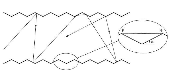
Figure 2.1: Particle bouncing in a pipeline with serrated triangular boundaries.

In the literature, one encounters examples of particle dynamics on bounded domains where the random perturbation is introduced in the observations of $\theta_{out}$ every time the particles bounces off the wall (see for example [5]), which implies that collisions are no longer elastic. This perturbation is explained as a consequence of the roughness of the wall. Observe that, in our model, randomness is introduced in a completely different way. We assume elastic collisions but, instead of considering dispersive geometries responsible for the random bounces, the noise is introduced in a sensible way without modifying the (rather elementary) geometry of the problem.

The trajectory that a particle describes after it comes out of a billiard cell until it enters another one on the opposite wall is completely irrelevant for dynamical purposes. In practice, we can better understand our dynamical system as the closed billiard table obtained by fixing together two triangular cells so that they share the same open side as in Figure 2.2. When the particle crosses that open side, it retains its direction but it is assigned a different position on $\overline{pq}$ according to a uniform law.

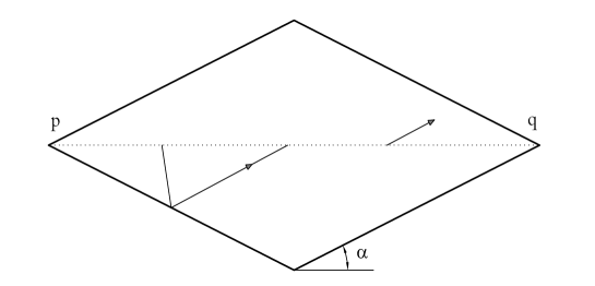
Figure 2.2: Fundamental cell. A particle crosses the open side $\overline{pq}$ at a uniformly distributed random point.

The incoming angle $\theta_{in}$ (resp. outgoing angle) is then the angle in $[-\pi/2,\pi/2]$ with which the particle enters (resp. leaves) the cell measured with respect to the normal to the open side $\overline{pq}$. One often shifts $[-\pi/2,\pi/2]$ by $\pi/2$ and measure $\theta$ in $[0,\pi]$, i.e. with respect to horizontal. In [7], for any incoming angle $\theta\in[0,\pi]$, Feres gives the different possible directions with which a particle may come out of the fundamental cell (Fig. 2.2). They are four, given by maps $\tau_{i}:[0,\pi]\rightarrow\mathbb{R}$ defined as

$$\tau_{1}\left(\theta\right) =\theta+2\alpha,~{}~{}\tau_{2}\left(\theta\right)=-\theta+2\pi-4\alpha$$

$$\tau_{3}\left(\theta\right) =\theta-2\alpha,~{}~{}\tau_{4}\left(\theta\right)=-\theta+4\alpha,$$ (M1)

and any $\tau_{i}$ applies with certain probability $p_{i}$. The probabilities associated to the maps (M1) are as follows:

$$p_{1}\left(\theta\right) =\left\{\begin{array}[c]{ll}1&\theta\in[0,\alpha)\\ u_{\alpha}\left(\theta\right)&\theta\in[\alpha,\pi-3\alpha)\\ 2\cos(2\alpha)u_{2\alpha}(\theta)&\theta\in[\pi-3\alpha,\pi-2\alpha)\\ 0&\theta\in[\pi-2\alpha,\pi]\end{array}\right.\vskip 3.0pt plus 1.0pt minus 1.0pt$$ (2.5)

$$p_{2}\left(\theta\right) =\left\{\begin{array}[c]{ll}0&\theta\in[0,\pi-3\alpha)\\ u_{\alpha}\left(\theta\right)-2\cos(2\alpha)u_{2\alpha}(\theta)&\theta\in[\pi-3\alpha,\pi-2\alpha)\\ u_{\alpha}\left(\theta\right)&\theta\in[\pi-2\alpha,\pi-\alpha)\\ 0&\theta\in[\pi-\alpha,\pi]\end{array}\right.\vskip 3.0pt plus 1.0pt minus 1.0pt$$ (2.10)

$$p_{3}\left(\theta\right) =\left\{\begin{array}[c]{ll}0&\theta\in[0,2\alpha)\\ 2\cos(2\alpha)u_{2\alpha}(-\theta)&\theta\in[2\alpha,3\alpha)\\ u_{\alpha}\left(-\theta\right)&\theta\in[3\alpha,\pi-\alpha)\\ 1&\theta\in[\pi-\alpha,\pi]\end{array}\right.\vskip 3.0pt plus 1.0pt minus 1.0pt$$ (2.15)

$$p_{4}\left(\theta\right) =\left\{\begin{array}[c]{ll}0&\theta\in[0,\alpha)\\ u_{\alpha}\left(-\theta\right)&\theta\in[\alpha,2\alpha)\\ u_{\alpha}\left(-\theta\right)-2\cos(2\alpha)u_{2\alpha}(-\theta)&\theta\in[2\alpha,3\alpha)\\ 0&\theta\in[3\alpha,\pi],\end{array}\right.$$ (M2)

where

$$u_{\alpha}\left(\theta\right)=\frac{1}{2}\left(1+\frac{\tan\alpha}{\tan\theta}\right)$$ (2.20)

and $\alpha$ is assumed to be smaller than $\pi/6$. As we will see later, this family of maps and probabilities is all we need to prove Knudsen’s law.

3 Preliminaries on Billiard Dynamics

This section aims at recalling the main concepts of the theory of (deterministic) billiards and one of its key results, namely, that the billiard map preserves the Liouville measure. The content of this section was extracted from [3], which the reader is referred to for an exhaustive exposition on billiards.

A billiard table $D$ is the closure of a bounded open domain $D_{0}\subset\mathbb{R}^{2}$ whose boundary $\partial D=\Gamma_{1}\cup\cdots\cup\Gamma_{m}$ is a finite union of smooth compact curves ($C^{l}$, $l\geq 3$). $\Gamma_{1},...,\Gamma_{n}$ are called the walls of the billiard table and are assumed to intersect each other only at their endpoints or corners. For any $i=1,...,n$, $\Gamma_{i}$ is defined by a $C^{l}$ map $f_{i}:[a_{i},b_{i}]\subset\mathbb{R}\rightarrow\mathbb{R}^{2}$ such that the second derivative $f_{i}^{\prime\prime}$ either vanishes or is identically zero. This condition prevents the wall $\Gamma_{i}$ from having inflection points or line segments. A wall such that $f^{\prime\prime}\neq 0$ is called focusing or dispersing if $f^{\prime\prime}$ points inwards or outwards $D$, respectively. Otherwise $f^{\prime\prime}=0$ and the wall is called flat. In this framework, we consider the dynamics of a point particle moving freely within $D$.

Let $q\in D$ denote the position of a free particle moving within a billiard table. We suppose that the particle bounces at $\partial D$ elastically. That is, if it collides with the wall $\Gamma$ at a point $p$ that is not a corner, the incident angle $\theta_{in}$ that the velocity $v$ forms with the normal vector $n$ to $\Gamma$ at $p$ equals the angle of reflection $\theta_{ref}$ between $n$ and $v$ after the collision, i.e. $\theta_{in}=\theta_{ref}$. This implies that $v$ has constant norm, which we will assume equal to $1$ for the sake of simplicity. Under these assumptions, the billiard flow $\Phi$ is the flow that this particle defines on the phase space $D\times\mathbb{S}^{1}$. Since the particle follows a straight trajectory between two consecutive collisions, the dynamical information of the system is contained in the geometry of the boundary $\partial D$ and how the particle bounces off it. Therefore, instead of studying the billiard flow, first one introduces the cross-section $M=\partial D\times[-\pi/2,\pi/2]$ as the set of all postcollisional velocity vectors, where $\theta\in[-\pi/2,\pi/2]$ measures the angle between $v$ and the normal vector $n$ pointing to the interior of $D$, and then considers the first return map $F$ that the billiard flow induces on $M$. That is, given a point of $M$, $F$ gives the next position at where the particle collides and its velocity after that collision. The map $F$ is often called the billiard map.

It is a well known result in the theory of billiards that the billiard map preserves the Liouville measure $\lambda\otimes\mu$ on $M$, where $\lambda$ is the Lebesgue measure on $\partial D$ and $\mu$ is the measure on $[-\pi/2,\pi/2]$ given by $\mu(A)=\frac{1}{2}\int_{A}\cos(\theta)d\theta$, $A\subseteq\mathcal{B}\left([-\pi/2,\pi/2]\right)$ ([3, Lemma 2.35]). However, except for a few general results, little is known about the ergodicity of billiard maps with respect to the Liouville measure for explicit examples of boundary geometries. For example, dispersive billiards are ergodic ([3, Theorem 6.20]) while regular polygons are not.

Finally, as we pointed out in Section 2, it is customary in the literature to translate $[-\pi/2,\pi/2]$ and measure $\theta$ in $[0,\pi]$, in which case $\mu$ is given by $\mu(A)=\frac{1}{2}\int_{A}\sin(\theta)d\theta$, $A\subseteq\mathcal{B}\left([0,\pi]\right)$. We will follow this convention throughout the paper.

4 First Return Map. Random Billiards

In this section we are going to get back to the concept of random billiard and its different representations.

Let $D$ be a billiard table with boundary $\partial D=\Gamma_{1}\cup\cdots\cup\Gamma_{m}$. Remove one of the walls of $\partial D$, for example $\Gamma_{1}$, so that we obtain a billiard table with an open side. Without loss of generality, we can assume that the open side is just a line segment $\overline{pq}$ as in Figure 2.2. This identification can be carried out by the map $f_{1}:[a_{1},b_{1}]\subset\mathbb{R}\rightarrow\mathbb{R}^{2}$ defining $\Gamma_{1}$. On the other hand, suppose a particle enters the billiard from the open side at $x\in\overline{pq}$ with an angle $\theta_{in}\in[0,\pi]$ with respect to $\Gamma_{1}$. Denote by $\Psi_{x}(\theta_{in})\in[0,\pi]$ the angle associated to the velocity of that particle when it returns to the open side for the first time. The first return map (to the open side) is then the map $T:\overline{pq}\times[0,\pi]\rightarrow\overline{pq}\times[0,\pi]$ induced from the billiard map $F$ such that $T\left(x,\theta_{in}\right)=\left(y,\Psi_{x}(\theta_{in})\right)$, i.e., the particle leaves the billiard at $y\in\overline{pq}$ with an angle $\theta_{out}=\Psi_{x}(\theta_{in})$.

The Liouville measure $\lambda\otimes\mu$ on $\partial D\times[0,\pi]$ induces a measure on $\overline{pq}\times[0,\pi]$ by restriction in a natural way. We will continue referring to this measure as the Liouville measure and denoting it by $\lambda\otimes\mu$, where $\lambda$ now stands for the Lebesgue measure on $\overline{pq}$. It can be proved that the first return map $T$ also preserves the Liouville measure ([4, Exercise I.5.1]). Furthermore,

Lemma 1

If the billiard map $F:\partial D\times[0,\pi]\rightarrow\partial D\times[0,\pi]$ is ergodic with respect to $\lambda\otimes\mu$, so is the first return map $T:\overline{pq}\times[0,\pi]\rightarrow\overline{pq}\times[0,\pi]$.

Proof. Let $A\in\mathcal{B}(\overline{pq})\otimes\mathcal{B}([0,\pi])$ be an invariant set, i.e., $T^{-1}\left(A\right)=A$. This set can be naturally regarded as a measurable set of $\partial D\times[0,\pi]$ since $\overline{pq}\subset\partial D$ is identified with the wall $\Gamma_{1}$. Since $F$ is ergodic, ${\textstyle\bigcup\nolimits_{n\geq 1}}F^{-n}\left(A\right)$ has full $\left.\lambda\otimes\mu\right|_{\partial D\times[0,\pi]}$-measure, which means that

$$\left.\lambda\otimes\mu\right|_{\partial D\times[0,\pi]}(({\textstyle\bigcup\nolimits_{n\geq 1}}F^{-n}\left(A\right))\bigcap\left(\overline{pq}\times[0,\pi]\right))=1.$$

If $y\in F^{-n}\left(A\right)\bigcap\left(\overline{pq}\times[0,\pi]\right)$, then $y=F^{-n}\left(x\right)$ for some $x\in A$ and, from the very definition of the first return map that, $y=T^{-m_{n}}\left(x\right)$ for some $m_{n}\leq n$. Therefore,

$$\left(\bigcup\nolimits_{n\geq 1}F^{-n}\left(A\right)\right)\bigcap\left(\overline{pq}\times[0,\pi]\right)=\bigcup\nolimits_{m\geq 1}T^{-m}\left(A\right)=A,$$

where the last equality follows from the invariance of $A$. Consequently, $\left.\lambda\otimes\mu\right|_{\overline{pq}\times[0,\pi]}(A)=1$ and $T$ is ergodic.  

Let $\left(\overline{pq},\mathcal{B}(\overline{pq}),\lambda\right)$ be the probability space built upon $\overline{pq}$ with the normalised Lebesgue measure $\lambda$ on the Borel $\sigma$-algebra $\mathcal{B}(\overline{pq})$. The random billiard associated to $D$ is then the time-discrete random dynamical system $\left\{\Psi_{x}:[0,\pi]\rightarrow[0,\pi]~{}|~{}x\in\overline{pq}\right\}$, where $\overline{pq}$ is regarded as a probability space. Roughly speaking, the random billiard thus built models the outgoing state a free particle that entered the billiard through the open side at a point uniformly distributed along $\overline{pq}$. When regarded as a probability space, $\overline{pq}$ will be denoted by $\Omega$.

The random billiard $\left\{\Psi_{x}:[0,\pi]\rightarrow[0,\pi]~{}|~{}x\in\Omega\right\}$ defines a transition probability kernel $K:[0,\pi]\times\mathcal{B}\left([0,\pi]\right)\rightarrow[0,1]$ given by

$$K(\theta,A)=\lambda\left(\{x\in\Omega~{}|~{}\Psi_{x}(\theta)\in A\}\right)\text{, where }x\in[0,\pi]\text{ and }A\in\mathcal{B}\left([0,\pi]\right).$$ (4.1)

We say that $\nu$ is invariant with respect to $\left\{\Psi_{x}:[0,\pi]\rightarrow[0,\pi]~{}|~{}x\in\Omega\right\}$ if

$$\nu(A)=\int_{[0,\pi]}K(\theta,A)d\nu(\theta)\text{ for any }A\in\mathcal{B}\left([0,\pi]\right)$$

and that the random billiard is ergodic with respect to $\nu$ if $T$ is ergodic with respect to $\lambda\otimes\nu$. For example, $\mu(A)=\frac{1}{2}\int_{A}\sin\theta d\theta$, $A\in\mathcal{B}\left([0,\pi]\right)$, is an invariant measure because $\lambda\otimes\mu$ is invariant with respect to the first return map $T$ ([7, Proposition 2.1]). Moreover, since dispersive billiards are ergodic with respect to the Liouville measure, the corresponding random billiard is also ergodic with respect to $\mu$ (Lemma 1). In this situation, Birkhoff’s Ergodic Theorem implies that

$$\frac{1}{n}\sum_{i=1}^{n}\mathbf{1}_{A}\left(\pi_{2}\circ T^{n}\right)\underset{n\rightarrow\infty}{\longrightarrow}\frac{1}{2}\int_{A}\sin(\theta)d\theta\text{~{}~{}a.s.,}$$ (4.2)

where $\pi_{2}:\overline{pq}\times[0,\pi]\rightarrow[0,\pi]$ is the projection onto the second factor. That is, the average number of particles reflected with some angle $\theta\in A$ converges to $\frac{1}{2}\int_{A}\sin(\theta)d\theta$ so (weak) Knudsen’s law holds for dispersive billiards.

In general, for non-dispersive billiards, little is know about the ergodicity of the first return map. This is indeed the case of the random billiard introduced in Section 2 (Fig. 2.2). Recall that, as far as we know, determining whether a general irrational triangular billiard is ergodic is still an open problem ([9, Section 7]) and only a few particular examples were proved to be ergodic ([14]). Therefore, at this point, it is not clear at all if Knudsen’s law holds for the pipeline model introduced in Section 2. To prove it, the first return map must be replaced with a more convenient representation.

5 Skew-Type Representation of Random Maps

Given a random billiard, the probability kernel (4.1) contains all the dynamical information of the system and determines its properties. This implies that, as far as the dynamics is concerned, the underlying probability space $\Omega$ (which in Section 4 was equal to $\left(\overline{pq},\mathcal{B}(\overline{pq}),\lambda\right)$) plays a secondary role. In particular, other probability spaces $\left(\Omega,\mathcal{F},P\right)$ giving rise to the same probability kernel are available. Indeed, if $K:X\times\mathcal{B}\rightarrow[0,1]$ is a transition probability kernel on a measurable space $\left(X,\mathcal{B}\right)$, Kolmogorov’s Existence Theorem on Markov processes guarantees that there exists a probability $P$ defined on the Borel $\sigma$-algebra of the topological space $\Omega={\textstyle\prod\nolimits_{i=1}^{\infty}}X_{i}$, $X_{i}:=X$ for all $i\geq 1$, such that the chain $\Phi_{i}:=\pi_{i}$ is Markovian and has transition probability kernel $K$ ([2, Theorem 2.11]), where $\pi_{i}:{\textstyle\prod\nolimits_{i=1}^{\infty}}X_{i}\rightarrow X$ is the projection onto the $i$th factor. In this statement, $X$ has to be a $\sigma$-compact Hausdorff space and $\mathcal{B}$ the Borel $\sigma$-algebra. Unfortunately, ${\textstyle\prod\nolimits_{i=1}^{\infty}}X_{i}$ is not very manageable to work with explicitly. For instance, the representation $T:\overline{pq}\times[0,\pi]\rightarrow\overline{pq}\times[0,\pi]$ given by the first return map introduced in Section 4 only involves finite dimensional spaces and hence seems more convenient. We are now going to consider another skew-type representation for random maps recently introduced in [1]. As we will show in Section 7, this representation will be crucial to prove the asymptotic properties of the random map defined by our random billiard Fig. 2.2.

Let $\left(X,\mathcal{B},\nu\right)$ be a general measure space and let $\left([0,1),\mathcal{B}\left([0,1)\right),\lambda\right)$ be the unit interval regarded as a probability space, where $\lambda$ stands for the Lebesgue measure. Later on, we will apply the results of this section to $X=[0,\pi]$. For any $k=1,...,N$, let $\tau_{k}:X\rightarrow X$ and $p_{k}:X\rightarrow[0,1]$ be measurable mappings such that $\{p_{k}\}_{k=1,...,N}$ is a measurable partition of the unity, i.e., $\sum_{k=1}^{N}p_{k}(x)=1$ for any $x\in X$ (compare to (M2) and (M1) in Section 2). We define the random dynamical system $\tau:X\rightarrow X$ such that $\tau\left(x\right)=\tau_{i}\left(x\right)$ with probability $p_{i}\left(x\right)$. The transition probability kernel of $\tau$ is given by

$$K\left(x,A\right)=\sum_{i=1}^{N}p_{i}\left(x\right)\mathbf{1}_{A}\left(\tau_{i}(x)\right).$$ (5.1)

This probability kernel defines the evolution of an initial distribution (probability measure) $\nu$ on $\left(X,\mathcal{B}\right)$ under the random map $\tau$ iteratively as

$$\nu^{(0)}:=\nu,~{}~{}\nu^{(n+1)}(A)=\int_{[0,\pi]}K(\theta,A)d\nu^{(n)}(\theta),~{}~{}n\geq 1,$$ (5.2)

where $A\in\mathcal{B}$. A measure $\nu$ is called invariant if $\nu^{(1)}=\nu$.

Following [1], consider now $\Omega=[0,1)\times X$ and set $J_{k}:=\{(y,x)\in\Omega~{}|~{}\sum_{i<k}p_{i}(x)\leq y<\sum_{i\leq k}p_{i}(x)\}$ such that $\{J_{k}\}_{k=1,...,N}$ is a finite measurable partition of $\Omega$. We define the skew-type representation of the random map $\tau$ as the map $S:[0,1)\times X\rightarrow[0,1)\times X$ such that

$$S\left(y,x\right)=\left(\varphi_{k}(y,x),\tau_{k}(x)\right)\text{ for }\left(y,x\right)\in J_{k}$$ (5.3)

where

$$\varphi_{k}\left(y,x\right)=\frac{1}{p_{k}(x)}\left(y-\sum_{i=1}^{k-1}p_{i}(x)\right).$$

The map $\varphi_{k}$ is well defined because if $\left(y,x\right)\in J_{k}$ then $p_{k}(x)>0$ necessarily. Moreover, $S$ thus defined is $\mathcal{B}\left([0,1)\right)\otimes\mathcal{B}$-measurable ([1, Lemma 3.1]) and it is a skew-type representation of the random dynamical system $\tau$.

As we will see, the map $S$ is extremely useful to study the properties of $\tau$. For example, $\nu$ is an invariant measure of $\tau$ on $\left(X,\mathcal{B}\right)$ if and only if $\lambda\otimes\nu$ is an invariant measure of $S$ on $\left([0,1)\times X,\mathcal{B}\left([0,1)\right)\otimes\mathcal{B},\lambda\otimes\nu\right)$ ([1, Lemma 3.2]). Moreover, since we know that the sine $\mu(A)=\frac{1}{2}\int_{A}\sin(\theta)d\theta$ is invariant by the transition probability kernel (5.1) of our billiard table, we conclude that $\mu$ is invariant by $\tau$ built from (M2) and (M1), and therefore $\lambda\otimes\mu$ is invariant by the corresponding map $S$. In an abuse of terminology, we will continue calling $\lambda\otimes\mu$ the Liouville measure when referring to $S$. In this context, we will say that the random map $\tau$ with initial distribution $\nu$ is ergodic (resp. mixing, exact) if $S$ is ergodic (resp. mixing, exact) with respect to $\lambda\otimes\nu$. In Section 7, we are going to prove that the $S$ associated to (M2) and (M1) is exact.

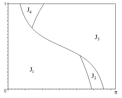
Figure 5.1: The sets $J_{i}$, $i=1,...,4$, for the random dynamical system defined in Section 2.

Unlike the first return map $T$ (Section 4), the map $S$ has no dynamical interpretation and is a purely auxiliary tool to represent and study $\tau$. Therefore, we need to establish the relationship between $S$ and the transition probability kernel (5.1), which carries all the dynamical information. This is the content of Theorem 4. Before stating that relationship, we need to introduce some notation and an auxiliary lemma, whose proof is included separately in the Appendix for the sake of a clearer exposition.

Definition 2

We define iteratively the sets $J_{i_{1}\cdots i_{n}}$, where $i_{j}\in\{1,...,N\}$ for any $j=1,...,n$, as

$$J_{i_{1}\cdots i_{n}}:=\left\{\omega\in J_{i_{n}}~{}|~{}S\left(\omega\right)\in J_{i_{n-1}},S^{2}\left(\omega\right)\in J_{i_{n-2}},....,S^{n-1}(\omega)\in J_{i_{1}}\right\}.$$ (5.4)

Lemma 3

Let $I_{x}:=[0,1)\times\{x\}$ the fibre through $x\in X$.  If $I_{x}\bigcap J_{i_{1}\cdots i_{n}}\neq\emptyset$, then

$$\lambda\left(\pi_{1}\left(I_{x}\bigcap J_{i_{1}\cdots i_{n}}\right)\right)=p_{i_{n}}(x)p_{i_{n-1}}\left(\tau_{i_{n}}(x)\right)\cdots p_{i_{1}}(\tau_{i_{2}}\circ\cdots\circ\tau_{i_{n}}(x)).$$

Theorem 4

Let $\nu$ be a measure on $\left(X,\mathcal{B}\right)$ and $A\in\mathcal{B}$. Then,

$$\operatorname*{E}\nolimits_{\lambda\otimes\nu}\left[\mathbf{1}_{A}\left(\pi_{2}\circ S^{n}\right)\right]:=\int_{[0,1)\times X}\mathbf{1}_{A}\left(\pi_{2}\circ S^{n}\right)d\left(\lambda\otimes\nu\right)=\nu^{(n)}\left(A\right).$$

Proof. First of all, it is not difficult to check that

$$\nu^{(n)}\left(A\right)=\sum_{i_{1},...,i_{n}}\int dv\left(x\right)p_{i_{n}}\left(x\right)p_{i_{n-1}}\left(\tau_{i_{n}}\left(x\right)\right)\cdots p_{i_{1}}\left(\tau_{i_{2}}\circ...\circ\tau_{i_{n}}(x)\right)\mathbf{1}_{A}\left(\tau_{i_{1}}\circ...\circ\tau_{i_{n}}(x)\right).$$

This can be proved iteratively rewriting $K$ in terms of (auxiliary) Dirac deltas, $K\left(x,dy\right)=\sum_{i=1}^{K}p_{i}\left(x\right)\delta\left(y-\tau_{k}\left(x\right)\right)dy$ where $\int f\left(y\right)\delta\left(y-a\right)dy=f\left(a\right)$, $f\in C\left(\mathbb{R}\right)$.

On the other hand, since $[0,1)\times X=\bigcup\nolimits_{i_{1},...,i_{n}}J_{i_{1}...i_{n}}$ is the disjoint union of the sets $J_{i_{1}...i_{n}}$, $i_{j}\in\{1,...,N\}$,

$$\int_{[0,1)\times X}\mathbf{1}_{A}\left(\pi_{2}\circ S^{n}\right)d\left(\lambda\otimes\nu\right) =\sum_{i_{1},...,i_{n}}\int_{J_{i_{1}...i_{n}}}\mathbf{1}_{A}\left(\pi_{2}\circ S^{n}\right)d\left(\lambda\otimes\nu\right)$$

$$=\sum_{i_{1},...,i_{n}}\int_{J_{i_{1}...i_{n}}}\mathbf{1}_{A}\left(\tau_{i_{1}}\circ...\circ\tau_{i_{n}}\right)d\left(\lambda\otimes\nu\right)$$

$$=\sum_{i_{1},...,i_{n}}\int_{[0,1)\times X}\mathbf{1}_{J_{i_{1}...i_{n}}}\mathbf{1}_{A}\left(\tau_{i_{1}}\circ...\circ\tau_{i_{n}}\right)d\left(\lambda\otimes\nu\right),$$

where, in the second line, we have used that $\mathbf{1}_{A}\left(\pi_{2}\circ S^{n}\right)=\mathbf{1}_{A}\left(\tau_{i_{1}}\circ...\circ\tau_{i_{n}}\right)$ on the set $J_{i_{1}...i_{n}}$. If now we apply Fubini’s theorem,

$$\int_{[0,1)\times X}\mathbf{1}_{J_{i_{1}...i_{n}}}\mathbf{1}_{A}\left(\tau_{i_{1}}\circ...\circ\tau_{i_{n}}\right)d\left(\lambda\otimes\nu\right)=\int_{X}\mathbf{1}_{A}\left(\tau_{i_{1}}\circ...\circ\tau_{i_{n}}(x)\right)dv\left(x\right)\int_{[0,1)}\mathbf{1}_{J_{i_{1}...i_{n}}}\left(y,x\right)d\lambda\left(y\right),$$

but by Lemma 3, for any fixed $x\in X$,

$$\int_{[0,1)}\mathbf{1}_{J_{i_{1}...i_{n}}}\left(y,x\right)d\lambda\left(y\right)=p_{i_{n}}(x)\cdots p_{i_{1}}(\tau_{i_{2}}\circ\cdots\circ\tau_{i_{n}}(x)).$$

Therefore,

$$\int_{[0,1)\times X}\mathbf{1}_{A}\left(\pi_{2}\circ S^{n}\right)d\left(\lambda\otimes\nu\right)=\sum_{i_{1},...,i_{n}}\int_{X}p_{i_{n}}\left(x\right)\cdots p_{i_{1}}\left(\tau_{i_{2}}\circ...\circ\tau_{i_{n}}(x)\right)\mathbf{1}_{A}\left(\tau_{i_{1}}\circ...\circ\tau_{i_{n}}(x)\right)dv\left(x\right).$$

 

Corollary 5

Let $U_{S}:L^{p}\left([0,1)\times X,\lambda\otimes\mu\right)\rightarrow L^{p}\left([0,1)\times X,\lambda\otimes\mu\right)$, $p\geq 1$, be the Koopman operator associated to $S$, i.e., $U_{S}f=f\circ S$. Let $\pi_{2}:[0,1)\times X\rightarrow X$ be the projection onto the second factor. If $\nu$ is a measure on $\left(X,\mathcal{B}\right)$, then

$$\nu^{(n)}\left(A\right)=\int_{[0,1)\times[0,\pi]}U_{S}^{n}\left(1_{\pi_{2}^{-1}(A)}\right)d\left(\lambda\otimes\nu\right),~{}A\in\mathcal{B},~{}n\in\mathbb{N}.$$

Let $S$ be the skew-type representation of the random billiard introduced in Section 2 and let $\nu\ll\mu$ be a probability measure absolutely continuous with respect to the Liouville measure $\mu$ with Radon-Nikodym derivative $f\in L^{1}\left([0,\pi],\mu\right)$. One can easily check that $\frac{d\left(\lambda\otimes\nu\right)}{d\left(\lambda\otimes\mu\right)}=\pi_{2}^{\ast}(f)$, where $\pi_{2}^{\ast}(f)\left(\omega\right):=f\left(\pi_{2}\left(\omega\right)\right)$ and $\omega\in[0,1)\times[0,\pi]$. If $S$ is mixing (or exact) then, from Corollary 5,

$$\int\pi_{2}^{\ast}\left(f\right)U_{S}^{n}\left(1_{\pi_{2}^{-1}(A)}\right)d\left(\lambda\otimes\mu\right)\underset{n\rightarrow\infty}{\longrightarrow}\int\pi_{2}^{\ast}\left(f\right)d\left(\lambda\otimes\mu\right)\int\mathbf{1}_{\pi_{2}^{-1}\left(A\right)}d\left(\lambda\otimes\mu\right)=\mu\left(A\right)$$ (5.5)

([12, Proposition 4.4.1 (b)]), which implies the strong Knudsen’s law. We will prove that $S$ is exact in Section 7 and give more details about the strong law in Section 8. The proof uses the fact that the pull-back $\pi_{2}^{\ast}\left(\mathbf{1}_{C}\right)$ of a characteristic function $\mathbf{1}_{C}$, $C\in\mathcal{B}\left(\left[0,\pi\right]\right)$, cannot be invariant by $S^{2}:=S\circ S$ (Section 6). It is worth observing that the strong law, unlike the standard approach to random billiards available in the literature from the first return map (see 4.2), is a consequence of the asymptotic properties of the skew-type representation $S$.

6 Properties of $S^{2}$

Let $S$ be the skew-type representation of the random map (M1) and (M2). In this section, we are going to show that $S^{2}=S\circ S:[0,1)\times[0,\pi]\rightarrow[0,1)\times[0,\pi]$ cannot leave invariant any characteristic function $\pi_{2}^{\ast}\left(\mathbf{1}_{C}\right)$, where $C\in\mathcal{B}\left(\left[0,\pi\right]\right)$ has probability $0<\mu\left(C\right)<1$ and $\pi_{2}:[0,1)\times X\rightarrow X$ denotes the projection onto the second factor. This result will be used in the next section to prove that $S$ is exact. First, we will show that our model exhibits a very useful symmetry.

Proposition 6

Let $S$ be the skew-type representation of the random map (M1) and (M2). Let $g:[0,\pi]\rightarrow\mathbb{R}$ be a function such that $\pi_{2}^{\ast}(g)$ is $S^{2}$-invariant, i.e.,

$$\pi_{2}^{\ast}(g)=\pi_{2}^{\ast}(g)\circ S^{2},$$ (6.1)

and let $\phi:[0,\pi]\rightarrow[0,\pi]$ be defined by $\theta\mapsto\pi-\theta$. Then $\pi_{2}^{\ast}(g\circ\phi)$ is also $S^{2}$-invariant.

Proof. It is not difficult to realise from (M2) that

$$p_{1}\circ\phi=p_{3},~{}~{}p_{3}\circ\phi=p_{1},~{}\text{~{}}p_{2}\circ\phi=p_{4},\text{ and }p_{4}\circ\phi=p_{2}$$

just using that the the function $u_{\alpha}(\theta)$ introduced in (2.20) has period $\pi$. Furthermore, straightforward computations shows that

$$\phi\circ\tau_{1}\circ\phi=\tau_{3},~{}~{}\phi\circ\tau_{3}\circ\phi=\tau_{1},~{}~{}\phi\circ\tau_{2}\circ\phi=\tau_{4},\text{ and }\phi\circ\tau_{4}\circ\phi=\tau_{2}.$$

Given an index $k\in\{1,...,4\}$, we define its conjugate index $\widetilde{k}$ in the following manner:

$$\widetilde{1}=3,~{}~{}\widetilde{3}=1,~{}~{}\widetilde{2}=4,\text{ and }\widetilde{4}=2.$$

On the other hand, (6.1) is equivalent to

$$g\left(x\right)=g\left(\tau_{j}\left(\tau_{i}(x)\right)\right)\text{ if }p_{i}\left(x\right)p_{j}\left(\tau_{i}\left(x\right)\right)>0.$$ (6.2)

We have to check that this property holds for $g\circ\phi$. So let $x\in[0,\pi]$ such that $p_{i}\left(x\right)p_{j}\left(\tau_{i}\left(x\right)\right)>0$. Since $p_{i}=p_{\widetilde{i}}\circ\phi$ and $\phi\circ\tau_{{}_{\widetilde{i}}}=\tau_{i}\circ\phi$ for any $i=1,...,4$, we have that $p_{i}\left(x\right)p_{j}\left(\tau_{i}\left(x\right)\right)>0$ implies

$$\left.\begin{array}[c]{r}p_{i}\left(x\right)=p_{\widetilde{i}}\circ\phi\left(x\right)>0\\ p_{j}\left(\tau_{i}\left(x\right)\right)=p_{\widetilde{j}}\circ\phi\circ\tau_{i}\left(x\right)=p_{\widetilde{j}}\circ\tau_{{}_{\widetilde{j}}}\circ\phi\left(x\right)>0\end{array}\right\}\Longrightarrow(p_{\widetilde{i}}\cdot(p_{\widetilde{j}}\circ\tau_{{}_{\widetilde{j}}}))\circ\phi\left(x\right)>0.$$

Therefore, using the invariance of $g$ expressed in (6.2)

$$g\left(\phi(x)\right)=g\left(\tau_{\widetilde{j}}\circ\tau_{\widetilde{i}}\circ\phi(x)\right)=g\left(\tau_{\widetilde{j}}\circ\phi\circ\tau_{i}(x)\right)=\left(g\circ\phi\right)\left(\tau_{j}\circ\tau_{i}(x)\right),$$

so $g\circ\phi$ also satisfies (6.2) and is $S^{2}$-invariant.   

Proposition 7

Let $g\in L^{1}\left([0,\pi],\mu\right)$ and suppose that $\pi_{2}^{\ast}(g)$ is invariant by $S^{2}$ and $\phi$. If $\alpha$ in (M2) and (M1) is irrational, then $g$ is constant.

Proof. Let $\left.[0,\pi]\right/_{0\sim\pi}$ be the quotient space obtained by identifying $0\sim\pi$. This space is homeomorphic to the unit circle $\mathbb{S}^{1}$. The function $g:[0,\pi]\rightarrow\mathbb{R}$ induces a function $[g]:\left.[0,\pi]\right/_{0\sim\pi}-\{[0]\}\rightarrow\mathbb{R}$ on the quotient that is well defined except at $[0]$, the equivalence class of $0$, because maybe $g(0)\neq g\left(\pi\right)$. We are going to prove that $[g]$ is invariant by an irrational rotation. Since constants are the only integrable functions invariant by irrational rotations, $[g]$ must be constant and $g$ too.

Recall that $\pi_{2}^{\ast}\left(g\right)=\pi_{2}^{\ast}\left(g\right)\circ S^{2}$ reads as

$$g\left(x\right)=g\left(\tau_{j}\left(\tau_{i}(x)\right)\right)\text{ if }p_{i}\left(x\right)p_{j}\left(\tau_{i}\left(x\right)\right)>0.$$ (6.2)

We are going split the interval $\left[0,\pi\right]$ into subintervals and, for each of them, we will explore the invariance properties of $g$ implied by (6.2).

(i)

If $x\in(0,\pi-4\alpha)$, then $p_{1}\left(x\right)p_{1}\left(\tau_{1}\left(x\right)\right)=p_{1}\left(x\right)p_{1}\left(x+2\alpha\right)>0$ so

$$g\left(x\right)=g\left(\tau_{1}\left(\tau_{1}(x)\right)\right)=g\left(x+4\alpha\right).$$

(ii)

If $x\in[\pi-4\alpha,\pi-3\alpha)$, then $p_{1}\left(x\right)p_{2}\left(\tau_{1}\left(x\right)\right)=p_{1}\left(x\right)p_{2}\left(x+2\alpha\right)>0$. Writing $x=\pi-4\alpha+z$ with $z\in[0,\alpha)$,

$$g\left(\pi-4\alpha+z\right)=g\left(\tau_{2}\left(\tau_{1}(\pi-4\alpha+z)\right)\right)=g\left(\pi-2\alpha-z\right).$$

Now, since $g$ is $\phi$-invariant,

$$g\left(\pi-2\alpha-z\right)=g\left(\phi\left(\pi-2\alpha-z\right)\right)=g\left(2\alpha+z\right)$$

Therefore,

$$\left[g\right]\left(\left[x\right]\right)=\left[g\right]\left(\left[x+6\alpha\right]\right)\text{ if }x\in[\pi-4\alpha,\pi-3\alpha).$$

(iii)

If $x\in[\pi-3\alpha,\pi-2\alpha)$ then $p_{2}\left(x\right)p_{3}\left(\tau_{2}\left(x\right)\right)>0$. Writing $x=\pi-2\alpha-z$ with $z\in[0,\alpha)$,

$$g\left(\pi-2\alpha-z\right)=g\left(\tau_{3}\left(\tau_{2}(\pi-2\alpha-z)\right)\right)=g\left(\pi-4\alpha+z\right).$$

Using $g=g\circ\phi$,

$$g\left(\pi-4\alpha+z\right)=g\left(\phi\left(\pi-4\alpha+z\right)\right)=g\left(4\alpha-z\right).$$

That is,

$$\left[g\right]\left(\left[x\right]\right)=\left[g\right]\left(\left[x+6\alpha\right]\right)\text{ if }x\in[\pi-3\alpha,\pi-2\alpha).$$

(iv)

Suppose $x\in[\pi-2\alpha,\pi-\alpha)$, $x=\pi-2\alpha+z$ with $z\in[0,\alpha)$. Since $p_{2}\left(x\right)p_{1}\left(\tau_{2}\left(x\right)\right)>0$ on $[\pi-2\alpha,\pi-\alpha)$, by (6.2),

$$g\left(x\right)=g\left(\tau_{2}\circ\tau_{1}(x)\right),~{}~{}\tau_{2}\circ\tau_{1}(x)=\pi-z.$$

Since $g$ is invariant by $\phi$,

$$g(\pi-z)=g\left(\phi\left(\pi-z\right)\right)=g\left(z\right),~{}~{}z\in[0,\alpha).$$

Summarising, $g\left(\pi-2\alpha+z\right)=g(z)$ which implies

$$[g]\left([x]\right)=[g]\left([x+2\alpha]\right)\text{ if }x\in[\pi-2\alpha,\pi-\alpha).$$

Now $z\in[0,\alpha)$ and we can use the $S^{2}$-invariance expressed in the first item so that

$$\left[g\right]\left(\left[x\right]\right)=\left[g\right]\left(\left[x+2\alpha\right]\right)=\left[g\right]\left(\left[x+6\alpha\right]\right).$$

(v)

Finally, let $x\in[\pi-\alpha,\pi)$, $x=\pi-\alpha+z$ with $z\in[0,\alpha)$. Since $p_{3}\left(x\right)p_{2}\left(\tau_{3}\left(x\right)\right)>0$ on $[\pi-\alpha,\pi)$

$$g\left(x\right)=g\left(\tau_{2}\circ\tau_{3}(x)\right),~{}~{}\tau_{2}\circ\tau_{3}(x)=\pi-\alpha-z.$$

by (6.2). Using the $\phi$-invariance of $g$,

$$g(\pi-\alpha-z)=g\left(\phi\left(\pi-\alpha-z\right)\right)=g\left(z+\alpha\right).$$

That is, $g\left(x\right)=g(z+\alpha)$, which again implies

$$[g]\left([x]\right)=[g]\left([x+2\alpha]\right)\text{ if }x\in[\pi-\alpha,\pi).$$

Now $x+2\alpha\in[\alpha,2\alpha)$ and $2\alpha<\pi-4\alpha$ as by assumption $\alpha<\pi/6$; we are in the situation of (i) so

$$\left[g\right]\left(\left[x\right]\right)=\left[g\right]\left(\left[x+2\alpha\right]\right)=\left[g\right]\left(\left[x+6\alpha\right]\right).$$

In conclusion, if $g$ is invariant by $S^{2}$ and $\phi$, then

$$\left[g\right]\left(\left[x\right]\right)=\left\{\begin{array}[c]{l}\left[g\right]\left(\left[x+4\alpha\right]\right)\text{ \ if }x\in(0,\pi-4\alpha)\\ \left[g\right]\left(\left[x+6\alpha\right]\right)\text{ \ if }x\in[\pi-4\alpha,\pi).\end{array}\right.$$ (6.3)

Let $k\in\mathbb{N}$ such that $\left(4k+6\right)\alpha>\pi>\left(4\left(k-1\right)+6\right)\alpha$. Observe that $k\geq 1$ because $\alpha<\pi/6$. Applying the invariance expressed in (6.3) iteratively, we have

$$\left[g\right]\left(\left[x\right]\right)=\left[g\right]\left(\left[x+\left(4k+6\right)\alpha\right]\right)\text{ for any }x\in\left(0,\pi\right).$$ (6.4)

In other words, $\left[g\right]$ is invariant by the rotation of angle $\left(4k+6\right)\alpha$. If $\alpha/2\pi$ is irrational, $g$ must be constant.   

Proposition 8

Let $C\in\mathcal{B}\left([0,\pi]\right)$ and suppose that $\pi_{2}^{\ast}(\mathbf{1}_{C})$ is $S^{2}$-invariant. If $\alpha$ in (M2) and (M1) is irrational, then $\mu\left(C\right)$ equals either $1$ or $0$.

Proof. Suppose that $0<\mu\left(C\right)<1$. We want to prove that $\pi_{2}^{\ast}(\mathbf{1}_{C})$ cannot be $S^{2}$-invariant. Since constants are trivially $S^{2}$-invariant, we can subtract $\mu\left(C\right)$ from $\mathbf{1}_{C}$ so that $\mathbf{1}_{C}-\mu\left(C\right)$ is still $S^{2}$-invariant and has expectation $0$. Let $g:=\mathbf{1}_{C}-\mu\left(C\right)$ and define $\overline{g}:=\frac{1}{2}\left(g+g\circ\phi\right)$, which is clearly $\phi$-invariant because $\phi^{2}=\operatorname*{Id}$. Since $\pi_{2}^{\ast}(g)$ is $S$-invariant, so are $\pi_{2}^{\ast}(g\circ\phi)$ (Proposition 6) and $\pi_{2}^{\ast}(\overline{g})$. By Proposition 7, $\overline{g}$ is constant and equal to its expectation $\operatorname*{E}_{\mu}\left[\overline{g}\right]$. But $\operatorname*{E}\nolimits_{\mu}\left[g\circ\phi\right]=\operatorname*{E}\nolimits_{\mu}\left[g\right]=0$ because $d\mu=\sin\left(x\right)dx$ and $\sin\left(x\right)$ are invariant by $\phi$. Therefore, $\operatorname*{E}_{\mu}\left[\overline{g}\right]=0$ and $\overline{g}$, which is constant, must be equal to $0$. That is,

$$g=-g\circ\phi.$$ (6.5)

Since

$$g\left(x\right)=\mathbf{1}_{C}\left(x\right)-\mu\left(C\right)=\left\{\begin{array}[c]{l}1-\mu\left(C\right)>0\text{ if }x\in C\\ -\mu\left(C\right)<0\text{ if }x\notin C,\end{array}\right.$$

(remember that we assumed $0<\mu\left(C\right)<1$), we conclude from (6.5) that $1-\mu\left(C\right)=-\left(-\mu\left(C\right)\right)\Longrightarrow\mu\left(C\right)=1/2$ and

$$\begin{array}[c]{l}g\left(x\right)=1/2\Longleftrightarrow x\in C,\\ g(x)=-1/2\Longleftrightarrow x\in C^{c}.\end{array}$$

Moreover, looking carefully at the proof of Proposition 7, we have

$$\left[g\right]\left(\left[x\right]\right)=\left\{\begin{array}[c]{l}\left[g\right]\left(\left[x+4\alpha\right]\right)\text{ \ if }x\in(0,\pi-4\alpha)\\ -\left[g\right]\left(\left[x+6\alpha\right]\right)\text{ \ if }x\in[\pi-4\alpha,\pi),\end{array}\right.$$

where instead of $g=g\circ\phi$ we have now used $g=-g\circ\phi$. Therefore, (see (6.4))

$$\left[g\right]\left(\left[x\right]\right)=-\left[g\right]\left(\left[x+\left(4k+6\right)\alpha\right]\right)\text{ for any }x\in(0,\pi),$$ (6.6)

where $k\geq 1$ is such that $\left(4k+6\right)\alpha>\pi>\left(4\left(k-1\right)+6\right)\alpha$. The minus sign in (6.6) tells us that the rotation $R_{\beta}$ of angle $\beta:=\left(4k+6\right)\alpha-\pi$ sends $C$ to $C^{c}$ and vice versa.

Let $\mathbf{1}_{C}=\sum_{n=-\infty}^{\infty}a_{n}\operatorname*{e}\nolimits^{2inx}$ and $\mathbf{1}_{C^{c}}=\sum_{n=-\infty}^{\infty}\widetilde{a}_{n}\operatorname*{e}\nolimits^{2inx}$ the Fourier expansions of $\mathbf{1}_{C}$ and $\mathbf{1}_{C^{c}}$ respectively. Since $\mathbf{1}_{C}+\mathbf{1}_{C^{c}}=\mathbf{1}_{[0,\pi]}$, we have that

$$\widetilde{a}_{n}=-a_{n}\text{ if }n\neq 0$$

$$a_{0}+\widetilde{a}_{0}=1.$$

On the other hand, we already argued that $\mathbf{1}_{C}\circ R_{\beta}=\mathbf{1}_{C^{c}}$. Imposing that the Fourier coefficients of $\mathbf{1}_{C}$ and $\mathbf{1}_{C^{c}}$ are unique, we deduce that

$$a_{n}\operatorname*{e}\nolimits^{2in\beta}=\widetilde{a}_{n}=-a_{n}\text{ for any }n\neq 0.$$

As $\beta/2\pi$ is irrational, $\operatorname*{e}\nolimits^{2in\beta}\neq-1$ for any $n\neq 0$, which implies that $a_{n}=0$ for any $n\neq 0$ so $\mathbf{1}_{C}$ is constant a.s.. But this is clearly a contradiction because (6.5) implied $\mu\left(C\right)=1/2$.   

7 Exactness of $S$

In this section, we are going to prove that $S$ is exact. This will imply Knudsen’s strong law for the random billiard introduced in Section 2.

Let $T:\Omega\rightarrow\Omega$ be a measurable transformation of a probability space $\left(\Omega,\mathcal{F},\mu\right)$. From the measurability of $T$, we have the chain of $\sigma$-algebras

$$...\subseteq T^{-n}\left(\mathcal{F}\right)\subseteq...\subseteq T^{-2}\left(\mathcal{F}\right)\subseteq T^{-1}\left(\mathcal{F}\right)\subseteq\mathcal{F}.$$ (7.1)

The map $T$ is called exact if the $\sigma$-algebra $\mathcal{G}:=\bigcap\nolimits_{n\geq 0}T^{-n}\left(\mathcal{F}\right)$ only contains sets of measure either $0$ or $1$. It is not difficult to prove that sets in $\mathcal{G}$ are characterised by the property

$$A\in\mathcal{G}\Longleftrightarrow A=T^{-n}\left(T^{n}\left(A\right)\right)\text{ for any }n\in\mathbb{N}.$$

This characterisation, in turn, implies that a map $T$ is exact if and only if

$$\lim_{n\rightarrow\infty}\mu\left(T^{n}\left(A\right)\right)=1$$

for any $A\in\mathcal{\mathcal{F}}$ such that $\mu\left(A\right)>0$ ([13, Section 2.2]). Equation (7.1) reads at the level of $L^{2}$ spaces as

$$...\subseteq U_{T}^{n}L^{2}\subseteq...\subseteq U_{T}^{2}L^{2}\subseteq U_{T}L^{2}\subseteq L^{2}$$

where $L^{2}=L_{\mathbb{C}}^{2}\left(\Omega,\mathcal{F},\mu\right)$ and $U_{T}\left(f\right)=f\circ T$ is the Koopman operator defined on $L^{2}$. If a map is exact, then

$$\bigcap\nolimits_{n=0}^{\infty}U_{T}^{n}L^{2}=\mathbb{C},$$

which means that $U_{T}^{n}\left(f\right)\rightarrow\operatorname*{E}_{\mu}\left[f\right]$ in $L^{2}$ as $n\rightarrow\infty$ (see [13, Section 2.5]). If $\nu$ is a probability absolutely continuous with respect to $\mu$ with Radon-Nikodym derivative $f\in L^{1}$, then

$$T_{\ast}^{n}\nu\left(A\right)=\operatorname*{E}\nolimits_{\mu}\left[fU_{T}^{n}\left(\mathbf{1}_{A}\right)\right]\underset{n\rightarrow\infty}{\longrightarrow}\mu\left(A\right)\operatorname*{E}\nolimits_{\mu}\left[f\right]=\mu(A),$$

that is, the sequence of measures $T_{\ast}^{n}\nu$ converges (weakly) to $\mu$ for any absolutely continuous measure $\nu\ll\mu$ ([12, Proposition 4.4.1 (b)], [13, Section 2.6]).

We want to show that the skew-type representation $S:[0,1)\times[0,\pi]\rightarrow[0,1)\times[0,\pi]$ of the model introduced in Section 2 is exact with respect to the Liouville measure to conclude that, for any absolutely continuous measure $\nu\ll\mu$ on $\mathcal{B}\left([0,\pi]\right)$ and any $A\in\mathcal{B(}[0,\pi])$,

$$\nu^{(n)}\left(A\right)=\int_{[0,\pi]}\mathbf{1}_{A}\left(\pi_{2}\circ S^{n}\right)d\nu=\int_{[0,\pi]}U_{S}^{n}\left(\mathbf{1}_{\pi_{2}^{-1}(A)}\right)d\lambda\otimes\nu\underset{n\rightarrow\infty}{\longrightarrow}\mu\left(A\right),$$ (7.2)

i.e., that the strong Knudsen’s law holds. Observe from (7.2) that we only need to consider the action of the Koopman operator $U_{S}$ on square integrable functions that are the pull-back by $\pi_{2}$ of functions in $L_{\mathbb{C}}^{2}\left([0,\pi],\mathcal{B}\left([0,\pi]\right),\mu\right)$. We are going to denote $L_{\mathbb{C}}^{2}\left([0,\pi],\mathcal{B}\left([0,\pi]\right),\mu\right)$ simply by $L^{2}\left([0,\pi]\right)$ for the sake of a clearer notation. Consequently, we do not need to check that $S$ is exact for the Borel $\sigma$-algebra of $[0,1)\times[0,\pi]$ but it is enough to consider a smaller one, namely, the smallest $\sigma$-algebra that makes both the functions in $\pi_{2}^{\ast}\left(L^{2}\left([0,\pi]\right)\right)$ and $S$ measurable.

Definition 9

For any $n\in\mathbb{N}$, let

$$\mathcal{F}_{n}:=\sigma\left(\left\{\pi_{2}^{-1}\left(U\right)\bigcap J_{i_{1}...i_{n}}~{}|~{}U\in\mathcal{B}\left([0,\pi]\right)\right\}\right),$$

where $J_{i_{1}...i_{n}}$ are as in Definition 2. For any $U\in\mathcal{B}\left([0,\pi]\right)$, the sets $\pi_{2}^{-1}\left(U\right)\bigcap J_{i_{1}...i_{n}}$ and $\pi_{2}^{-1}\left(U\right)$ will be called generators (of $\mathcal{F}_{n}$).

The sequence of $\sigma$-algebras $\left\{\mathcal{F}_{n}\right\}_{n\in\mathbb{N}}$ define a filtration,

$$\mathcal{F}_{1}\subseteq\mathcal{F}_{2}\subseteq...\subseteq\mathcal{F}_{n}\subseteq...$$

Indeed, for any $U\in\mathcal{B}\left([0,\pi]\right)$ and any $n\geq 1$, a generator $\pi_{2}^{-1}\left(U\right)\bigcap J_{i_{1}...i_{n}}$ can be written as

$$\pi_{2}^{-1}\left(U\right)\bigcap J_{i_{1}...i_{n}}=\bigcup_{k=1}^{N}\left(\pi_{2}^{-1}\left(U\right)\bigcap J_{ki_{1}...i_{n}}\right),$$

which implies $\mathcal{F}_{n}\subseteq\mathcal{F}_{n+1}$. We define $\mathcal{F}$ as the limit of this filtration.

Definition 10

$$\mathcal{F}:=\sigma\left(\bigcup\nolimits_{n\geq 1}\mathcal{F}_{n}\right).$$

Proposition 11

$S:[0,1)\times[0,\pi]\rightarrow[0,1)\times[0,\pi]$ is $\mathcal{F}$-measurable. For any $f\in L^{2}\left([0,\pi]\right)$, $\pi_{2}^{\ast}\left(f\right)$ is also $\mathcal{F}$-measurable.

Proof. The second statement of the proposition is obvious. To prove that $S$ is $\mathcal{F}$-measurable it is enough to show that $S^{-1}\left(A\right)\in\mathcal{F}$ for the generators of $\mathcal{F}$. So let $A\in\mathcal{F}$ such that $A=\pi_{2}^{-1}\left(U\right)\bigcap J_{i_{1}...i_{n}}$ where $U\in\mathcal{B}\left([0,\pi]\right)$ and $n\geq 1$. Then, by definition of the sets $J_{i_{1}...i_{n}}$

$$S^{-1}\left(A\right)=\bigcup_{k=1}^{N}\left(\pi_{2}^{-1}\left(\tau_{k}^{-1}\left(U\right)\right)\bigcap J_{i_{1}...i_{n}k}\right)$$

which clearly belongs to $\mathcal{F}$.  

The following two lemmas aim at getting a better insight of the structure of the $\sigma$-algebra $\mathcal{F}$. As an immediate consequence of them, it will be enough to show that $S$ is exact by looking at its action on the generators of $\mathcal{F}$.

Lemma 12

Any set $A\in\mathcal{F}_{n}$ can be expressed as a finite union of disjoint generators.

Proof. First to all, observe that, for a fixed $n\in\mathbb{N}$, the sets $J_{i_{1}...i_{n}}$ are disjoint and form a partition of $[0,1)\times[0,\pi]$.

The complement of a generator $\pi_{2}^{-1}\left(U\right)\bigcap J_{i_{1}...i_{n}}$ is

$$\left(\pi_{2}^{-1}\left(U\right)\bigcap J_{i_{1}...i_{n}}\right)^{c}=\left(\biguplus_{j_{1}\neq i_{1},...,j_{n}\neq i_{n}}\pi_{2}^{-1}\left(U\right)\bigcap J_{j_{1}...j_{n}}\right)\biguplus\pi_{2}^{-1}\left(\left[0,\pi\right]\backslash U\right),$$

where $\biguplus$ denotes the disjoint union, so it can be expressed as a finite union of generators. On the other hand, if we take a countable union of generators $\left\{C_{k}\right\}_{k\geq 1}$, $C_{k}=\pi_{2}^{-1}\left(U_{k}\right)\bigcap J_{i_{1}^{k}...i_{n}^{k}}$,

$$\bigcup_{k\geq 1}\left(\pi_{2}^{-1}\left(U_{k}\right)\bigcap J_{i_{1}^{k}...i_{n}^{k}}\right)=\biguplus_{i_{1}^{k},...,i_{n}^{k}}\left(\bigcup\nolimits_{m\in I_{i_{1}^{k}...i_{n}^{k}}}\pi_{2}^{-1}\left(U_{m}\right)\right)\bigcap J_{i_{1}^{k}...i_{n}^{k}}$$

where $I_{i_{1}^{k}...i_{n}^{k}}:=\{k\geq 1~{}|~{}\pi_{2}^{-1}\left(U_{k}\right)\bigcap J_{i_{1}^{k}...i_{n}^{k}}$ is in $\left\{C_{m}\right\}_{m\geq 1}\}$. But

$$\biguplus_{i_{1}^{k},...,i_{n}^{k}}\left(\bigcup\nolimits_{m\in I_{i_{1}^{k}...i_{n}^{k}}}\pi_{2}^{-1}\left(U_{m}\right)\right)\bigcap J_{i_{1}^{k}...i_{n}^{k}}=\biguplus_{i_{1}^{k},...,i_{n}^{k}}\left(\pi_{2}^{-1}\left(\bigcup\nolimits_{m\in I_{i_{1}^{k}...i_{n}^{k}}}U_{k}\right)\right)\bigcap J_{i_{1}^{k}...i_{n}^{k}}.$$

where the indices $i_{1}^{k},...,i_{n}^{k}$ can only take finite number of possibilities. Therefore, a countable union of generators reduces to a finite union.  

The union $\bigcup\nolimits_{n\geq 1}\mathcal{F}_{n}$ of a filtration $\mathcal{F}_{1}\subseteq\mathcal{F}_{2}\subseteq...$ is an algebra of sets. The $\sigma$-algebra generated by an algebra of sets $\mathcal{A}$ is characterised by containing all the sets in $\mathcal{A}$ and the limit of all monotone sequence of sets. That is, $\sigma\left(\mathcal{A}\right)$ coincides with the monotone class generated by $\mathcal{A}$ ([6, Section 1.3, Theorem 1]). This observation is the key to proving the following Lemma:

Lemma 13

If $A\in\mathcal{F=}\sigma\left(\bigcup\nolimits_{n\geq 1}\mathcal{F}_{n}\right)$ has positive probability, then $A$ contains a generator of positive probability.

Proof. Let $A\in\sigma({\textstyle\bigcup\nolimits_{n\geq 1}}\mathcal{F}_{n})$. If $A\in\bigcup\nolimits_{n\geq 1}\mathcal{F}_{n}$, then $A\in\mathcal{F}_{n}$ for some $n\in\mathbb{N}$. By Proposition 12, $A$ can be expressed as a finite union of generators and at least one of them must have positive probability. If $A\notin\bigcup\nolimits_{n\geq 1}\mathcal{F}_{n}$, then there exists a monotone sequence of sets $\left\{B_{n}\right\}_{n\in\mathbb{N}}\subset\bigcup\nolimits_{n\geq 1}\mathcal{F}_{n}$ such that $A=\lim_{n}B_{n}$. We are going to deal with the cases $\left\{B_{n}\right\}_{n\in\mathbb{N}}$ increasing or decreasing separately.

• If $\left\{B_{n}\right\}_{n\in\mathbb{N}}$ is increasing, then $A=\bigcup\nolimits_{n\geq 1}B_{n}$. Since $\lambda\otimes\mu\left(A\right)>0$, at least one $B_{n}$ must have positive measure, $\lambda\otimes\mu\left(B_{n}\right)>0$. But $B_{n}\in\mathcal{F}_{m}$ for some $m$, so it contains a generator of positive probability.

• Let $\left\{B_{n}\right\}_{n\in\mathbb{N}}\subset\bigcup\nolimits_{n\geq 1}\mathcal{F}_{n}$ be a decreasing sequence such that $A=\bigcap\nolimits_{n\geq 1}B_{n}$. Suppose that $0<\mu\left(A\right)<1$ (otherwise there is nothing to prove). We have

  $$A=\left(\bigcup\nolimits_{n\geq 1}B_{n}^{c}\right)^{c}=\left(\left(\biguplus\nolimits_{n\geq 1}\left.B_{n+1}^{c}\right\backslash B_{n}^{c}\right)\biguplus B_{1}^{c}\right)^{c},$$

  so that $A$ can be expressed as the complement of a countable union of disjoint sets. Rename $C_{1}:=B_{1}^{c}$ and $C_{n}:=\left.B_{n+1}^{c}\right\backslash B_{n}^{c}$, and express any $C_{n}$ as a disjoint union of generators (Lemma 12),

  $$C_{n}=\biguplus_{r=1}^{k_{n}}\pi_{2}^{-1}\left(U_{r_{n}}\right)\bigcap J_{i_{1}^{n}...i_{r}^{n}}.$$

  In this decomposition, we only consider sets of strictly positive probability. Then,

  $$A^{c}=\biguplus_{n\geq 1}\biguplus_{r_{n}=1}^{k_{n}}\pi_{2}^{-1}\left(U_{r_{n}}\right)\bigcap J_{i_{1}^{n}...i_{r}^{n}}=\biguplus_{i_{1}^{n}...i_{r}^{n}}\left(\bigcup\nolimits_{m\in I_{i_{1}^{n}...i_{r}^{n}}}\pi_{2}^{-1}\left(U_{m}\right)\right)\bigcap J_{i_{1}^{n}...i_{r}^{n}}$$ (7.3)

  where $I_{i_{1}^{n}...i_{r}^{n}}:=\{m\geq 1~{}|~{}\pi_{2}^{-1}\left(U_{m}\right)\bigcap J_{i_{1}^{n}...i_{r}^{n}}\subseteq A^{c}=\biguplus\nolimits_{n}C_{n}\}$. We claim that there exists a generator $G$ of strictly positive probability that does not intersect $A^{c}$, i.e., $G\subseteq A$.

  Let $i_{1}^{n}...i_{r}^{n}$ be a sequence appearing in the decomposition (7.3). If $\mu(\bigcup\nolimits_{m\in I_{i_{1}^{n}...i_{r}^{n}}}U_{m})<1$, then

  $$\left(\left.\left[0,\pi\right]\right\backslash\pi_{2}^{-1}\left(\bigcup\nolimits_{m\in I_{i_{1}^{n}...i_{r}^{n}}}U_{m}\right)\right)\bigcap J_{i_{1}^{n}...i_{r}^{n}}$$

  is a generator of strictly positive measure that does not intersect $A^{c}$. If $\mu(\bigcup\nolimits_{m\in I_{i_{1}^{n}...i_{r}^{n}}}U_{m})=1$ for any finite sequence $i_{1}^{n}...i_{r}^{n}$ in (7.3), then $A^{c}=\biguplus_{i_{1}^{n}...i_{r}^{n}}J_{i_{1}^{n}...i_{r}^{n}}$ a.s. and since we assumed that $0<\mu\left(A^{c}\right)<1$, there must exist some set $J_{i_{1}...i_{k}}$ with positive probability that does not appear in the decomposition of $A^{c}$. That is, $J_{i_{1}...i_{k}}=\pi_{2}^{-1}\left([0,\pi]\right)\bigcap J_{i_{1}...i_{k}}\subseteq A$.

 

Theorem 14

For any $A\in\mathcal{F}$,

$$\lim_{n\rightarrow\infty}\lambda\otimes\mu\left(S^{n}\left(A\right)\right)=1.$$

In other words, $S:[0,1)\times[0,\pi]\rightarrow[0,1)\times[0,\pi]$ is an exact endomorphism of $\left([0,1)\times[0,\pi],\mathcal{F},\lambda\otimes\mu\right)$.

Proof. Let $A\in\mathcal{F}$ be such that $\lambda\otimes\mu\left(A\right)>0$. By Lemma 13, $A$ contains a generator $G=\pi_{2}^{-1}\left(U\right)\bigcap J_{i_{1}...i_{n}}$ of positive measure for some $U\in\mathcal{B}\left([0,\pi]\right)$, $n\geq 0$. It is an immediate consequence of the definitions that, after $n$ iterations, the set $S^{n}\left(G\right)$ has all its fibers of length $1$, that is,

$$\lambda\left(\left([0,1)\times\{x\}\right)\bigcap S^{n}\left(G\right)\right)=1\text{ for any }x=\tau_{i_{1}}\circ...\circ\tau_{i_{n}}\left(u\right),~{}u\in U.$$

Let $B:=S^{n}\left(G\right)$ and let $I_{x}:=[0,1)\times\{x\}$ be the fiber at $x\in[0,\pi]$. Looking carefully at (M1) and (M2), one can see that

$$\tau_{2}\circ\tau_{2}=\tau_{4}\circ\tau_{4}=\tau_{1}\circ\tau_{3}=\tau_{3}\circ\tau_{1}=\operatorname*{Id},$$

where $\operatorname*{Id}$ denotes the identity on $[0,\pi]$, and

$$p_{2}\left(x\right) >0\Rightarrow p_{2}\left(x\right)p_{2}\left(\tau_{2}\left(x\right)\right)>0$$

$$p_{4}\left(x\right) >0\Rightarrow p_{4}\left(x\right)p_{4}\left(\tau_{4}\left(x\right)\right)>0$$

$$p_{1}\left(x\right) >0\Rightarrow p_{1}\left(x\right)p_{3}\left(\tau_{1}\left(x\right)\right)>0$$

$$p_{3}\left(x\right) >0\Rightarrow p_{3}\left(x\right)p_{1}\left(\tau_{3}\left(x\right)\right)>0.$$

These remarks imply that, if $I_{x}\cap J_{i}\neq\emptyset$,

$$I_{x}\cap J_{i}\subseteq S^{2}\left(I_{x}\cap J_{i}\right).$$

Since all the fibers of $B$ have length $1$, $B\subseteq S^{2}\left(B\right)$ and, iteratively,

$$B\subseteq S^{2}\left(B\right)\subseteq...\subseteq S^{2n}\left(B\right)\subseteq...$$

Define $C:=\bigcup\nolimits_{n\geq 0}S^{2n}\left(B\right)$. Obviously $S^{2}\left(C\right)=C$, the fibers of $C$ have all length $1$, and $\lambda\otimes\mu\left(C\right)=\lim_{n\rightarrow\infty}\lambda\otimes\mu\left(S^{2n}\left(B\right)\right)$. We want to show that $\lambda\otimes\mu\left(C\right)=1$. Observe that $\lambda\otimes\mu\left(C\right)>0$ because $\lambda\otimes\mu\left(B\right)>0$. From $S^{2}\left(C\right)=C$ we have

$$C\subseteq S^{-2}\left(S^{2}\left(C\right)\right)=S^{-2}\left(C\right);$$

but $C$ and $S^{-2}\left(S^{2}\left(C\right)\right)$ have the same measure ($S^{2}$ is $\lambda\otimes\mu$-preserving), so $\mathbf{1}_{C}$ is a $S^{2}$-invariant function a.s.. Since $\mathbf{1}_{C}=\pi_{2}^{\ast}(\mathbf{1}_{\pi_{2}(C)})$ a.s. (the fibers of $C$ have all length $1$ a.s.), $\pi_{2}\left(C\right)$ has full measure by Proposition 8. Therefore, $\lambda\otimes\mu\left(C\right)=1$ and

$$\lim_{n\rightarrow\infty}S^{2n}\left(B\right)=1.$$

This proves that $S^{2}$ is exact. In general, we have

$$S^{2n}\left(B\right) \subseteq S^{-1}\left(S\left(S^{2n}\left(B\right)\right)\right)\subseteq S^{-1}\left(S^{2n+1}\left(B\right)\right)$$

$$S^{2n+1}\left(B\right) \subseteq S^{-1}\left(S\left(S^{2n+1}\left(B\right)\right)\right)\subseteq S^{-1}\left(S^{2(n+1)}\left(B\right)\right)$$

so that, using again that $S$ is $\lambda\otimes\mu$-preserving,

$$\lambda\otimes\mu\left(S^{2n}\left(B\right)\right)\leq\lambda\otimes\mu\left(S^{2n+1}\left(B\right)\right)\leq\lambda\otimes\mu\left(S^{2(n+1)}\left(B\right)\right),$$

which proves that $\left\{\lambda\otimes\mu\left(S^{n}\left(B\right)\right)\right\}_{n\in\mathbb{N}}$ is increasing and converges to $1$, i.e., $S$ is also exact.  

To sum up, the skew-type representation $S:[0,1)\times[0,\pi]\rightarrow[0,1)\times[0,\pi]$ associated to the random map (M1) and (M2) is exact which implies, by (7.2), that $\nu^{(n)}\rightarrow\mu$ as $n\rightarrow\infty$ for any initial distribution $\nu$ on $[0,\pi]$ absolutely continuous with respect to the law $\mu\left(A\right)=\frac{1}{2}\int_{A}\sin\left(\theta\right)d\theta$, $A\in\mathcal{B}\left([0,\pi]\right)$. Since $\sin\left(\theta\right)>0$ on $\left(0,\pi\right)$, $\mu$ and the Lebesgue measure $\lambda$ are absolutely continuous with respect to each other on $\left(0,\pi\right)$. In other words, strong Knudsen’s law $\nu^{(n)}\rightarrow\mu$ holds for any initial distribution absolutely continuous with respect to $\lambda$.

8 Knudsen’s law. Simulations

In this section, we are going to show that numerical simulations are in accordance with theoretical results. With this aim, we take an arbitrary initial distribution on $\left[0,\pi\right]$ such as in the following picture and we make it evolve according to our random system (M1) and (M2).

Initial normalised distribution of particles.

Since we can only simulate a finite number particles in a computer, in this experiment we take a total amount of 30000 balls and divide $\left[0,\pi\right]$ in subintervals of the same length (45 in our experiment). That is, we approximate the initial distribution by a step function. In each subinterval, we put the proportion of balls according to the probability density function above. The initial angle associated to any of those balls is the middle point of the interval where they fall. The simulation then goes as follows. At the $i$-th step, we take the $j$-th particle with angle $\theta_{j}^{(i)}$ and a random number $y_{j}^{(i)}$ uniformly distributed between $0$ and $1$, one for each particle. If $(y_{j}^{(i)},\theta_{j}^{(i)})\in J_{k}$, then $\theta_{j}^{(i+1)}=\tau_{k}(\theta_{j}^{(i)})$, where $\{\tau_{k}\}_{k=1,...,4}$ are as in (M1), and so on. After a long number of iterations, the distribution stabilises as follows:

Final normalised distribution of particles. In red, $\frac{1}{2}\sin(x)$.

As we can see, the outline of the final distribution tends to the graph of $\frac{1}{2}\sin\left(x\right)$. The small inaccuracy is explained by the fact that only a finite (i.e., a discrete) number of initial angles is considered. The smaller the subintervals in which $\left[0,\pi\right]$ is divided are, the better the final distribution approximates $\frac{1}{2}\sin\left(x\right)$. We have repeated this experiment over several initial distributions obtaining always similar results, which experimentally confirms the validity of Knudsen’s law for our model.

Appendix A Appendix

Proof of Lemma 3. To start with, will prove that

$$S\left(I_{x}\bigcap J_{i_{1}\cdots i_{n}}\right)=I_{\tau_{i_{n}}(x)}\bigcap J_{i_{1}\cdots i_{n-1}}.$$

From the very definition of $S$ and $J_{i_{1}\cdots i_{n}}$, we have

$$S\left(I_{x}\bigcap J_{i_{1}\cdots i_{n}}\right)\subseteq I_{\tau_{i_{n}}(x)}\bigcap J_{i_{1}\cdots i_{n-1}}.$$

On the other hand, let $\omega\in I_{\tau_{i_{n}}(x)}\bigcap J_{i_{1}\cdots i_{n-1}}$. Then $\omega=(y,\tau_{i_{n}}(x))$ for some $y\in[0,1)$. Let $\omega^{\prime}=(p_{i_{n}}(x)y+{\textstyle\sum\nolimits_{j=1}^{i_{n}-1}}p_{j}(x),x)$. It is obvious that $\omega^{\prime}\in J_{i_{n}}$ as $p_{i_{n}}(x)>0$ because $I_{x}\bigcap J_{i_{1}\cdots i_{n}}$ is not empty. Moreover, $S\left(\omega^{\prime}\right)=\omega$. Therefore $\omega\in S\left(I_{x}\bigcap J_{i_{1}\cdots i_{n}}\right)$ and

$$S\left(I_{x}\bigcap J_{i_{1}\cdots i_{n}}\right)\supseteq I_{\tau_{i_{n}}(x)}\bigcap J_{i_{1}\cdots i_{n-1}}.$$

Identifying both fibers $I_{x}\bigcap J_{i_{1}\cdots i_{n}}$ and $I_{\tau_{i_{n}}(x)}\bigcap J_{i_{1}\cdots i_{n-1}}$ as subsets of $[0,1)$, the map

$$\begin{array}[c]{rcl}S_{x}:I_{x}\bigcap J_{i_{1}\cdots i_{n}}\subset[0,1)&\longrightarrow&I_{\tau_{i_{n}}(x)}\bigcap J_{i_{1}\cdots i_{n-1}}\\ y&\longmapsto&\varphi_{i_{n}}(y,\tau_{i_{n}}(x))=\frac{1}{p_{i_{n}}(x)}\left(y-{\textstyle\sum\nolimits_{j=1}^{i_{n}-1}}p_{j}(x)\right),\end{array}$$ (A.1)

is then a diffeomorphism. After having identified $I_{x}\bigcap J_{i_{1}\cdots i_{n}}$ as a subset of $[0,1)$, we can compute its Lebesgue measure $\lambda\left(I_{x}\bigcap J_{i_{1}\cdots i_{n}}\right)$. Consequently,

$$\lambda\left(I_{x}\bigcap J_{i_{1}\cdots i_{n}}\right)=\int_{{}_{I_{x}\bigcap J_{i_{1}\cdots i_{n}}}}d\lambda=\int_{I_{\tau_{i_{n}}(x)}\bigcap J_{i_{1}\cdots i_{n-1}}}\frac{d(S_{x})^{-1}}{dy}d\lambda$$

$$=\int_{I_{\tau_{i_{n}}(x)}\bigcap J_{i_{1}\cdots i_{n-1}}}p_{i_{n}}(x)d\lambda=p_{i_{n}}(x)\int_{I_{\tau_{i_{n}}(x)}\bigcap J_{i_{1}\cdots i_{n-1}}}d\lambda$$

$$=p_{i_{n}}(x)\lambda\left(I_{\tau_{i_{n}}(x)}\bigcap J_{i_{1}\cdots i_{n-1}}\right).$$ (A.2)

Applying iteratively (A.2), we obtain

$$\lambda\left(I_{x}\bigcap J_{i_{1}\cdots i_{n}}\right)=p_{i_{n}}(x)p_{i_{n-1}}\left(\tau_{i_{n}}(x)\right)\cdots p_{1}(\tau_{i_{2}}\circ\cdots\circ\tau_{i_{n}}(x)).$$

 

Acknowledgements. The authors would like to thank Wael Bahsoun and Renato Feres for their enlightening comments and suggestions.

References

[1]W. Bahsoun, C. Bose, and A. Quas. Deterministic
representation for position dependent random maps. Discrete and
Continuous Dynamical Systems22 (3), 529-540, 2008.
[2]R. M. Blumenthal and R. K. Getoor. Markov
Processes and Potential Theory. Pure and Applied Mathematics. A Series of
Monographs and Textbooks, Vol. 29. Academic Press, 1968.
[3]N. Chernov and R. Markarian. Chaotic
Billiards, 3rd Edition. Mathematical Surveys and Monographs, vol.
127. American Mathematical Society, 2006.
[4]N. Chernov and R. Markarian.
Introduction to the Ergodic Theory of Chaotic Billiards.
Monografías del Instituto de Matemática y Ciencias Afines
19. Instituto de Matemática y Ciencias Afines; Pontificia
Universidad Católica del Perú, Lima, 2001.
[5]F. Comets, S. Popov, G. M. Schütz, and M. Vachkovskaia.
Billiards in a general domain with random reflections. Arch. Rational
Mech. Anal.191, 497–537, 2009.
[6]Y. S. Chow and H. Teicher.
Probability Theory: independence, interchangeability, martingales.
Springer-Verlag, 1978.
[7]R. Feres. Random walks derived from billiards.
Dynamics, ergodic theory, and geometry. Math. Sci. Res. Inst. Publ.
54, 179–222. Cambridge Univ. Press, Cambridge, 2007.
[8]R. Feres and G. Yablonsky. Knudsen’s cosine law
and random billiards. Chemical Engineering Sciences59,
1541-1556, 2001.
[9]A. Gorodnik. Open problems in dynamics and
related fields. Journal of Modern Dynamics1 (1), 1–35, 2007
[10]E. Gutkin. Billiard dynamics: a survey on
emphasis on open problems. Regular and Chaotic Dynamics8
(1), 2003.
[11]M. Knudsen. The Kinetic Theory of Gases, 1934.
[12]A. Lasota and M. Mackey. Probabilistic Properties of
Deterministic Systems. Cambridge University Press, 1985.
[13]V. A. Rohlin. Exact endomorphisms of a Lebesgue space.
Am. Math. Soc. Transl.Series 239, 1-36, 1964.
[14]Ya. B. Vorobets. Ergodicity of billiards in polygons.
Sbornik: Mathematics188 (3), 389-434, 1997