Frequency locking of modulated waves

Abstract.

We consider the behavior of a modulated wave solution to an $\mathbb{S}^{1}$-equivariant autonomous system of differential equations under an external forcing of modulated wave type. The modulation frequency of the forcing is assumed to be close to the modulation frequency of the modulated wave solution, while the wave frequency of the forcing is supposed to be far from that of the modulated wave solution. We describe the domain in the three-dimensional control parameter space (of frequencies and amplitude of the forcing) where stable locking of the modulation frequencies of the forcing and the modulated wave solution occurs.

Our system is a simplest case scenario for the behavior of self-pulsating lasers under the influence of external periodically modulated optical signals.

Lutz Recke

Institute of Mathematics, Humboldt University of Berlin,

Unter den Linden 6, 10099 Berlin, Germany

Anatoly Samoilenko, Alexey Teplinsky and Viktor Tkachenko,

Institute of Mathematics, National Academy of Sciences of Ukraine

3 Tereschenkivska St., 01601 Kiev, Ukraine

Serhiy Yanchuk

Institute of Mathematics, Humboldt University of Berlin,

Unter den Linden 6, 10099 Berlin, Germany

(Communicated by the associate editor name)

1. Introduction

This paper investigates systems of differential equations of the type

$$\frac{dx}{dt} = f(x)+g(x)|y|^{2},$$ (1.1)

$$\frac{dy}{dt} = h(x)y+\gamma e^{i\alpha t}a(\beta t),$$ (1.2)

where $x\in\mathbb{R}^{n},$ $y\in\mathbb{C}$, the functions $f,g:\mathbb{R}^{n}\to\mathbb{R}^{n},$ $h:\mathbb{R}^{n}\to\mathbb{C}$, and $a:\mathbb{R}\to\mathbb{C}$ are sufficiently smooth of class $C^{l}$ with some positive integer $l$. The function $a$ is $2\pi$-periodic, and $\alpha>0$, $\beta>0$ and $\gamma\geq 0$ are parameters. We assume that for $\gamma=0$ the unperturbed system

$$\frac{dx}{dt} = f(x)+g(x)|y|^{2},$$ (1.3)

$$\frac{dy}{dt} = h(x)y,$$ (1.4)

has an exponentially orbitally stable quasi-periodic solution of modulated wave type

$$x(t)=x_{0}(\beta_{0}t),\ y(t)=y_{0}(\beta_{0}t)e^{i\alpha_{0}t}.$$ (1.5)

Here $\alpha_{0}>0$ and $\beta_{0}>0$ are constants, while $x_{0}:\mathbb{R}\to\mathbb{R}^{n}$ and $y_{0}:\mathbb{R}\to\mathbb{C}$ are smooth $2\pi$-periodic functions. We assume that the following nondegeneracy condition holds:

$$\mbox{rank}\left[\begin{array}[]{cc}x_{0}^{\prime}(\psi)&0\\ \Re y_{0}^{\prime}(\psi)&-\Im y_{0}(\psi)\\ \Im y_{0}^{\prime}(\psi)&\Re y_{0}(\psi)\end{array}\right]=2.$$ (1.6)

It is easy to verify that (1.6) is true for all $\psi\in\mathbb{R}$ if it is true for one $\psi$. Moreover, without loss of generality we assume that $\psi\mapsto\arg y_{0}(\psi)$ is periodic, i.e. the curve $y=y_{0}(\psi)$ in $\mathbb{C}$ does not loop around the origin (otherwise we should replace $y_{0}(\beta_{0}t)$ by $y_{0}(\beta_{0}t)e^{ik\beta_{0}t}$ and $\alpha_{0}$ by $\alpha_{0}-k\beta_{0}$ with an appropriate $k\in\mathbb{Z}$).

It follows from assumption (1.6) that the set

$$\mathcal{T}_{2}:=\{(x_{0}(\psi),y_{0}(\psi)e^{i\varphi})\in\mathbb{R}^{n}\times\mathbb{C}:\;\varphi,\psi\in\mathbb{T}_{1}\},$$

where $\mathbb{T}_{1}=\mathbb{R}/(2\pi\mathbb{Z})$ is the unit circle, is diffeomorphic to a two-dimensional torus. Obviously, $\mathcal{T}_{2}$ is invariant with respect to the flow of (1.3)–(1.4), and the solution (1.5) lies on $\mathcal{T}_{2}$.

Roughly speaking, our main result describes the domain in the three-dimensional space of the control parameters $\alpha$, $\beta$ and $\gamma$ with $|\alpha-\alpha_{0}|\gg 1$ and $\beta\approx\beta_{0}$ such that the following holds: For almost any solution $(x(t),y(t))$ to (1.1)–(1.2), which is at a certain moment close to $\mathcal{T}_{2}$, there exists $\sigma\in\mathbb{R}$ such that

$$\|x(t)-x_{0}(\beta t+\sigma)\|+\bigl{|}|y(t)|-|y_{0}(\beta t+\sigma)|\bigr{|}\approx 0\mbox{ for large }t.$$

Let us reformulate our result in a more abstract language as well as in the language of a physical application.

Abstractly speaking, (1.3)–(1.4) is an autonomous system which is equivariant under the $\mathbb{T}_{1}$-action $(x,y)\mapsto(x,e^{i\varphi}y)$, $\varphi\in\mathbb{T}_{1}$, on the phase space. The solution (1.5) is a so-called modulated wave solution or relative periodic orbit to the $\mathbb{T}_{1}$-equivariant system (1.3)–(1.4). It is well-known that generically those solutions are structurally stable under small perturbations that do not destroy the autonomy and the $\mathbb{T}_{1}$-equivariance of the system. Thus, our results describe the behavior of exponentially orbitally stable modulated wave solutions to $\mathbb{T}_{1}$-equivariant systems under external forcings of modulated wave type in the case when the difference between the internal and the external modulation frequencies $\beta-\beta_{0}$ is small while the difference between the internal and the external wave frequencies $\alpha-\alpha_{0}$ is large. Note that in [12] related results are described for the case when both differences of modulation and wave frequencies are small, and [11] considers the case when the internal state as well as the external forcing are not modulated. For an even more abstract setting of these results see [4].

System (1.1)–(1.2) is a paradigmatic model for the dynamical behavior of self-pulsating lasers under the influence of external periodically modulated optical signals. For more involved mathematical models see, e.g., [1, 7, 8, 9, 10, 17, 18] and for related experimental results see [6, 15]. In (1.1)–(1.2), the state variables $x$ and $y$ describe the electron density and the optical field of the laser, respectively. In particular, the absolute value $|y|$ describes the intensity of the optical field. The $\mathbb{T}_{1}$-equivariance of (1.3)–(1.4) is the result of the invariance of autonomous optical models with respect to shifts of optical phases. The solution (1.5) describes a so-called self-pulsating state of the laser in the case when the laser is driven by electric currents which are constant in time. In those states the electron density and the intensity of the optical field are time periodic with the same frequency. Self-pulsating states usually appear as a result of Hopf bifurcations from so-called continuous wave states, where the electron density and the intensity of the optical field are constant in time.

The structure of our paper is as follows. The main results are formulated in Sec. 2. The proof is splitted into four sections. In Sec. 3 we use averaging transformations [2] in order to eliminate the fast oscillating terms with the frequency $\alpha$. It appears that the first non-vanishing terms after the averaging procedure are of order $\gamma^{2}/\alpha^{2}$. Local coordinates in the vicinity of the stable invariant toroidal manifold are introduced in Sec. 4 and then in Sec. 5 the existence of perturbed manifold is proved. The global behavior of a system on the perturbed torus is described in Sec. 6. Among others, the methods of perturbation theory [13, 14] are used in our analysis.

2. Main results

In new coordinates $x=x,y=re^{i\varphi}$, $r,\varphi\in\mathbb{R}$, the unperturbed system (1.3)–(1.4) has the form

$$\frac{dx}{dt}=f(x)+g(x)r^{2},$$ (2.1)

$$\frac{dr}{dt}=\Re h(x)r,$$ (2.2)

$$\frac{d\varphi}{dt}=\Im h(x).$$ (2.3)

This system has, by assumption, the two-frequency solution

$$x(t)=x_{0}(\beta_{0}t),\ r(t)=r_{0}(\beta_{0}t):=|y_{0}(\beta_{0}t)|,\ \varphi(t)=\alpha_{0}t+\arg y_{0}(\beta_{0}t).$$

The subsystem (2.1)–(2.2) does not depend on $\varphi$ and has an exponentially orbitally stable periodic solution $x(t)=x_{0}(\beta_{0}t),\ r(t)=r_{0}(\beta_{0}t).$ The corresponding variational system has the following form

$$\frac{dz}{d\psi}=A(\psi)z,\quad z\in\mathbb{R}^{n+1},$$ (2.4)

where

$$A(\psi):=\frac{1}{\beta_{0}}\left[\begin{array}[]{cc}{\displaystyle f^{\prime}(x_{0}(\psi))+g^{\prime}(x_{0}(\psi))r_{0}^{2}(\psi)}&{\displaystyle 2g(x_{0}(\psi))r_{0}(\psi)}\\[5.69054pt] {\displaystyle\Re h^{\prime}(x_{0}(\psi))r_{0}(\psi)}&{\displaystyle\Re h(x_{0}(\psi))}\end{array}\right].$$

We assume that

$$\left\{\begin{array}[]{l}\mbox{the trivial multiplier $1$ of the monodromy matrix of linear periodic}\\ \mbox{system (\ref{eq:VAR}) has multiplicity one, and the absolute values of all}\\ \mbox{other multipliers are less than $1$.}\end{array}\right.$$ (2.5)

The adjoint system

$$\frac{dp}{d\psi}=-A^{T}(\psi)p,$$

has a nontrivial periodic solution $p(\psi)$ ($A^{T}$ denotes the transpose of $A$), which can be normalized such that

$$p^{T}(\psi)\left[\begin{array}[]{c}x^{\prime}_{0}(\psi)\\ r^{\prime}_{0}(\psi)\end{array}\right]=1\mbox{ for all }\psi.$$

Let us define the function $\mathcal{G}:\mathbb{R}^{n}\times\mathbb{T}_{1}\to\mathbb{R}^{n+1}$ as follows

$${\mathcal{G}}(x,\psi):=\left[\begin{array}[]{c}g(x)|a(\psi)|^{2}\\ 0\end{array}\right].$$ (2.6)

Our first result describes the behavior (under the perturbation by the forcing term with $\gamma>0$) of $\mathcal{T}_{2}\times\mathbb{R}$, which is an integral manifold to (1.1)–(1.2) with $\gamma=0$, as well as the dynamics of the system (1.1)–(1.2) on the perturbed manifold.

Theorem 2.1.

Let us assume that the conditions (1.6) and (2.5) are met.

Then for all $\beta_{1}<\beta_{2}$ there exist positive constants $\mu_{*}$, $\alpha_{*}$, $\delta$, $L$ and $\kappa$ such that for all $(\alpha,\beta,\gamma)$ with

$$\alpha>\alpha_{*},\;\beta_{1}<\beta<\beta_{2}\mbox{ and }0\leq\frac{\gamma}{\alpha}<\mu_{*}$$ (2.7)

the following holds:

(i) The system (1.1)–(1.2) has a three-dimensional integral manifold $\mathfrak{M}(\alpha,\beta,\gamma)$ which can be parametrized by $\psi,\varphi,t\in\mathbb{R}$ in the form

$$x=x_{0}(\psi)+\frac{\gamma}{\alpha^{2}}X_{1}\left(\psi,\varphi,\beta t,\alpha t,\frac{1}{\alpha},\beta,\frac{\gamma}{\alpha}\right)+\frac{\gamma^{2}}{\alpha^{2}}X_{2}\left(\psi,\varphi,\beta t,\alpha t,\frac{1}{\alpha},\beta,\frac{\gamma}{\alpha}\right),$$

$$y=r_{0}(\psi)e^{i(\varphi+\phi(\psi))}-i\frac{\gamma}{\alpha}e^{i\alpha t}a(\beta t)+\frac{\gamma}{\alpha^{2}}Y_{1}\left(\psi,\varphi,\beta t,\alpha t,\frac{1}{\alpha},\beta,\frac{\gamma}{\alpha}\right)$$

$$\hskip 28.45274pt+\frac{\gamma^{2}}{\alpha^{2}}Y_{2}\left(\psi,\varphi,\beta t,\alpha t,\frac{1}{\alpha},\beta,\frac{\gamma}{\alpha}\right)\mbox{ \rm with }\phi(\psi):=\frac{1}{\beta_{0}}\int_{0}^{\psi}[\Im h(x_{0}(\xi))-\alpha_{0}]d\xi.$$

Here $X_{j}:\mathbb{R}^{4}\times U\to\mathbb{R}$ and $Y_{j}:\mathbb{R}^{4}\times U\to\mathbb{C}$ are $C^{l-4}$ smooth, $4\pi$-periodic with respect to $\psi$ and $2\pi$-periodic with respect to $\varphi,\beta t$ and $\alpha t$ and

$$U:=\left\{(\nu,\beta,\mu)\in\mathbb{R}^{3}:\;0<\nu<\frac{1}{\alpha_{*}},\;\beta_{1}<\beta<\beta_{2},\;0\leq\mu<\mu_{*}\right\}.$$

(ii) The dynamics of (1.1)–(1.2) on $\mathfrak{M}(\alpha,\beta,\gamma)$ in coordinates $\psi,\varphi$ and $t$ is determined by a system of the type

$$\frac{d\psi}{dt}=\beta_{0}+\frac{\gamma^{2}}{\alpha^{2}}p^{T}(\psi){\mathcal{G}}(x_{0}(\psi),\beta t)+\frac{\gamma^{4}}{\alpha^{4}}\Psi_{1}\left(\psi,\beta t,\frac{\gamma}{\alpha}\right)$$

$$\hskip 14.22636pt+\frac{\gamma^{2}}{\alpha^{3}}\Psi_{2}\left(\psi,\varphi,\beta t,\alpha t,\frac{1}{\alpha},\beta,\frac{\gamma}{\alpha}\right)+\frac{\gamma}{\alpha^{3}}\Psi_{3}\left(\psi,\varphi,\beta t,\alpha t,\frac{1}{\alpha},\beta,\frac{\gamma}{\alpha}\right),$$ (2.8)

$$\frac{d\varphi}{dt}=\alpha_{0}+\frac{\gamma^{2}}{\alpha^{2}}\Phi_{1}\left(\psi,\beta t,\frac{\gamma}{\alpha}\right)+\frac{\gamma^{2}}{\alpha^{3}}\Phi_{2}\left(\psi,\varphi,\beta t,\alpha t,\frac{1}{\alpha},\beta,\frac{\gamma}{\alpha}\right)$$

$$\hskip 71.13188pt+\frac{\gamma}{\alpha^{3}}\Phi_{3}\left(\psi,\varphi,\beta t,\alpha t,\frac{1}{\alpha},\beta,\frac{\gamma}{\alpha}\right),$$ (2.9)

where the functions $\Psi_{1},\Phi_{1}:\mathbb{R}^{2}\times[0,\mu_{*})\to\mathbb{R}$ and $\Psi_{j},\Phi_{j}:\mathbb{R}^{4}\times U\to\mathbb{R}$ $(j=2,3)$ are $C^{l-4}$-smooth, $4\pi$-periodic with respect to $\psi$ and $2\pi$-periodic with respect to $\varphi,\beta t$ and $\alpha t.$

(iii) The integral manifold $\mathfrak{M}(\alpha,\beta,\gamma)$ is exponentially attracting (uniformly with respect to $(\alpha,\beta,\gamma)$ satisfying (2.7)) in the following sense: For any solution $(x(t),y(t))$ to (1.1)–(1.2) such that $\mbox{\rm dist}((x(t_{0}),y(t_{0})),\mathcal{T}_{2})<\delta$ for certain $t_{0}\in\mathbb{R}$ there is a unique solution $(\psi(t),\varphi(t))$ to (2.8)– (2.9) such that

$$\Bigl{\|}x(t)-x_{0}(\psi(t))-\frac{\gamma}{\alpha^{2}}\tilde{X}_{1}(t)-\frac{\gamma^{2}}{\alpha^{2}}\tilde{X}_{2}(t)\Bigl{\|}+$$

$$+\Bigl{|}y(t)-i\frac{\gamma}{\alpha}e^{i\alpha t}a(\beta t)-r_{0}(\psi(t))e^{i(\varphi(t)+\phi(\psi(t)))}-\frac{\gamma}{\alpha^{2}}\tilde{Y}_{1}(t)-\frac{\gamma^{2}}{\alpha^{2}}\tilde{Y}_{2}(t)\Bigl{|}\leq$$

$$\leq Le^{-\kappa(t-t_{0})}\mbox{\rm dist}\left(\left(x(t_{0}),y(t_{0})\right),\mathcal{T}_{2}\right),\ t\geq t_{0},$$

where

$$\tilde{X}_{j}(t):=X_{j}\left(\psi(t),\varphi(t),\beta t,\alpha t,\frac{1}{\alpha},\beta,\frac{\gamma}{\alpha}\right),\quad j=1,2,$$

$$\tilde{Y}_{j}(t):=Y_{j}\left(\psi(t),\varphi(t),\beta t,\alpha t,\frac{1}{\alpha},\beta,\frac{\gamma}{\alpha}\right),\quad j=1,2.$$

Let us define the function

$$G(\psi):=\frac{1}{2\pi}\int_{0}^{2\pi}p^{T}(\psi+\theta){\mathcal{G}}(x_{0}(\psi+\theta),\psi)d\theta$$

and the numbers

$$G_{+}:=\max_{\psi\in[0,2\pi]}G(\psi),\quad G_{-}:=\min_{\psi\in[0,2\pi]}G(\psi).$$

For the sake of simplicity we will suppose that all singular points of $G$ are non-degenerate, i.e.

$$G^{\prime\prime}(\psi)\not=0\mbox{ for all }\psi\mbox{ such that }G^{\prime}(\psi)=0.$$ (2.10)

This implies that the set of singular points of $G$ consists of an even number $2N$ of different points:

$$\{\psi\in[0,2\pi):\,G^{\prime}(\psi)=0\}=\{\psi_{1},\ldots,\psi_{2N}\}.$$

The set of singular values of $G$ will be denoted by

$$S:=\{G(\psi_{1}),\ldots,G(\psi_{2N})\}.$$

The following two theorems describe the dynamics on $\mathfrak{M}(\alpha,\beta,\gamma)$ in more details. In particular, they show that for appropriate parameters $(\alpha,\beta,\gamma)$ there appears an even number of two-dimensional integral submanifolds, which determine the frequency locking behavior we are interested in.

Theorem 2.2.

Assume that (1.6), (2.5) and (2.10) hold.

Then for any $\varepsilon>0$ there exist positive $\mu^{*}$, $\mu_{*}$, and $\delta$ such that for all parameters $(\alpha,\beta,\gamma)$ satisfying

$$\frac{\mu^{*}}{\alpha}<\gamma<\mu_{*}\alpha,$$ (2.11)

$$G_{-}<\frac{\alpha^{2}}{\gamma^{2}}(\beta-\beta_{0})<G_{+},$$ (2.12)

$$\mathrm{\rm dist}\left(\frac{\alpha^{2}}{\gamma^{2}}\left(\beta-\beta_{0}\right),S\right)>\varepsilon$$ (2.13)

the following statements hold:

(i) The system (1.1)–(1.2) has an even number of two-dimensional integral manifolds $\mathfrak{N}_{j}(\alpha,\beta,\gamma)\subset\mathfrak{M}(\alpha,\beta,\gamma),\;j=1,...,2\hat{N}(\alpha,\beta,\gamma),\;0<\hat{N}(\alpha,\beta,\gamma)\leq N$ which can be parametrized by $\varphi,t\in\mathbb{R}$ in the form

$$x = x_{0}(\beta t+\vartheta_{j})+\frac{\gamma}{\alpha}X_{1j}\left(\varphi,\beta t,\alpha t,\frac{1}{\alpha},\beta,\frac{\gamma}{\alpha}\right)+\frac{1}{\alpha}X_{2j}\left(\varphi,\beta t,\alpha t,\frac{1}{\alpha},\beta,\frac{\gamma}{\alpha}\right),$$

$$y = r_{0}(\beta t+\vartheta_{j})e^{i\varphi+\phi(\beta t+\vartheta_{j})}$$

$$\hskip 42.67912pt+\frac{\gamma}{\alpha}Y_{1j}\left(\varphi,\beta t,\alpha t,\frac{1}{\alpha},\beta,\frac{\gamma}{\alpha}\right)+\frac{1}{\alpha}Y_{2j}\left(\varphi,\beta t,\alpha t,\frac{1}{\alpha},\beta,\frac{\gamma}{\alpha}\right),$$

where $\vartheta_{j}$ are constants, and the functions $X_{kj},Y_{kj}:\mathbb{R}^{4}\times V\to\mathbb{R}$ are $C^{l-4}$-smooth and $2\pi$-periodic with respect to $\varphi,\beta t$ and $\alpha t$, and

$$V:=\left\{(\nu,\beta,\mu):G_{-}<\mu^{2}(\beta-\beta_{0})<G_{+},\mu^{*}\nu^{2}<\mu<\mu_{*},\mbox{\rm dist}(\mu^{2}(\beta-\beta_{0}),S)>\varepsilon\right\}.$$

(ii) The dynamics of (1.1)–(1.2) on $\mathfrak{N}_{j}(\alpha,\beta,\gamma)$ in coordinates $\varphi$ and $t$ is determined by an equation of the type

$$\frac{d\varphi}{dt}=\alpha_{0}+\frac{\gamma^{2}}{\alpha^{3}}\Phi_{1j}\left(\varphi,\beta t,\alpha t,\frac{1}{\alpha},\beta,\frac{\gamma}{\alpha}\right)+\frac{\gamma}{\alpha^{3}}\Phi_{2j}\left(\varphi,\beta t,\alpha t,\frac{1}{\alpha},\beta,\frac{\gamma}{\alpha}\right),$$

where the functions $\Phi_{kj}:\mathbb{R}^{3}\times V\to\mathbb{R}$ are $C^{l-4}$ smooth and $2\pi$-periodic in $\varphi,\beta t$ and $\alpha t$.

(iii) Any solution $(x(t),y(t))$ to (1.1)–(1.2) such that $\mbox{\rm dist}((x(t_{0}),y(t_{0})),\mathcal{T}_{2})<\delta$ for certain $t_{0}\in\mathbb{R}$ tends to one of the manifolds $\mathfrak{N}_{j}(\alpha,\beta,\gamma)$ as $t\to\infty.$

Theorem 2.3.

Assume that (1.6), (2.5) and (2.10) hold.

Then for any $\varepsilon>0$ and $\varepsilon_{1}>0$ there exist positive $\mu^{*}$, $\mu_{*}$ and $\delta$ such that for all parameters $(\alpha,\beta,\gamma)$ satisfying the conditions (2.11)–(2.13) and for any solution $(x(t),y(t))$ of system (1.1)–(1.2) such that $\mbox{\rm dist}((x(t_{0}),y(t_{0})),\mathcal{T}_{2})<\delta$ for certain $t_{0}\in\mathbb{R}$ there exist $\sigma,T\in\mathbb{R}$ such that

$$\|x(t)-x_{0}(\beta t+\sigma)\|+\bigl{|}|y(t)|-|y_{0}(\beta t+\sigma)|\bigr{|}<\varepsilon_{1}\mbox{ for all }t>T.$$

The conditions (2.11)–(2.13) from Theorems 2.2 and 2.3 determine the so-called locking region, i.e. the set of all triples $(\alpha,\beta,\gamma)$ for which modulation frequency locking takes place. These domains are illustrated in the figures 1–4.

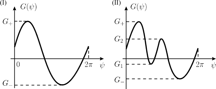
Figure 1. Graphs of the function $G$.

In Fig. 1 we show two typical cases of graphs of the function $G$. In the case (I) there exist one positive and one negative local extremum and in the case (II) two positive and two negative local extrema, i.e.,

$$\mbox{(I) }: \ N=1,\;S=\{G_{-},G_{+}\},\;G_{-}<0<G_{+},$$

$$\mbox{(II)}: \ N=2,\;S=\{G_{-},G_{1},G_{2},G_{+}\},\;G_{-}<G_{1}<0<G_{2}<G_{+}.$$

Figure 2. Cross-sections of the locking region $\alpha={\mathrm{c}onst}$.

In Fig. 2 we show $\alpha$=const sections of the locking region. In the case (I) this section is

$$\left\{(\beta,\gamma):\;\frac{\mu^{*}}{\alpha}<\gamma<\mu_{*}\alpha,\;G_{-}+\varepsilon<\frac{\alpha^{2}}{\gamma^{2}}(\beta-\beta_{0})<G_{+}-\varepsilon\right\}.$$

It is bounded by two straight lines $\gamma=\mu^{*}/\alpha$ and $\gamma=\mu_{*}\alpha$ and by two square root like curves

$$\gamma=\alpha\sqrt{\frac{\beta-\beta_{0}}{\tilde{G}}}\mbox{ with }\tilde{G}\in\{G_{-}+\varepsilon,G_{+}-\varepsilon\}.$$

In the case (II) the $\alpha$=const section is bounded by the same two horizontal straight lines and by six square root like curves

$$\gamma=\alpha\sqrt{\frac{\beta-\beta_{0}}{\tilde{G}}}\mbox{ with }\tilde{G}\in\{G_{-}+\varepsilon,G_{1}-\varepsilon,G_{1}+\varepsilon,G_{2}-\varepsilon,G_{2}+\varepsilon,G_{+}-\varepsilon\}.$$

Figure 3. Cross-sections of the locking region $\beta={\mathrm{const}}$.

Finally, in Fig. 3 we show $\beta$=const sections of the locking region in the $(1/\alpha,\gamma)$ plane. We consider the parameter $\alpha$ in the region $\alpha>\alpha_{*}$ with sufficiently large $\alpha_{*}>0$

$$\alpha_{*}^{2}>\frac{\mu^{*}}{\mu_{*}}\sqrt{\frac{G_{+}-\varepsilon}{G_{2}-\varepsilon}}.$$ (2.14)

If (2.14) is satisfied, consider the set of all $\beta>\beta_{0}$ such that

$$\frac{\mu^{*}}{\alpha_{*}}<\alpha_{*}\sqrt{\frac{\beta-\beta_{0}}{G_{+}-\varepsilon}}\mbox{ and }\sqrt{\frac{\beta-\beta_{0}}{G_{2}-\varepsilon}}<\mu_{*}.$$ (2.15)

For any fixed $\alpha>\alpha_{*}$, where $\alpha_{*}$ satisfies (2.14), and for any fixed $\beta>\beta_{0}$ with (2.15), the line $\{(\alpha,\beta,\gamma):\gamma\in\mathbb{R}\}$ crosses the boundary of the locking region in two points $\gamma=\mu_{1}\alpha$ and $\gamma=\mu_{*}\alpha$ in case (I) and in four points $\gamma=\mu_{1}\alpha$, $\gamma=\mu_{2}\alpha$, $\gamma=\mu_{3}\alpha$ and $\gamma=\mu_{*}\alpha$ in case (II) (see also Fig. 4). Here we denoted

$$\mu_{1}=\sqrt{\frac{\beta-\beta_{0}}{G_{+}-\varepsilon}},\;\mu_{2}=\sqrt{\frac{\beta-\beta_{0}}{G_{2}+\varepsilon}},\;\mu_{3}=\sqrt{\frac{\beta-\beta_{0}}{G_{2}-\varepsilon}}.$$

Figure 4. Intersection of a line $\beta={\mathrm{const}}$ with the boundary of the locking region.

3. Averaging

In this section we perform changes of variables with the aim to average the nonautonomous terms with fast oscillating arguments $\alpha t$. As the result of these transformations, we obtain an equivalent system, where the fast oscillating terms have the order of magnitude of $\gamma^{2}/\alpha^{2}$ and smaller. The principles and details of the averaging procedure can be found e.g. in [2].

Performing the change of variables

$$x = x_{1},$$

$$y = y_{1}-i\frac{\gamma}{\alpha}e^{i\alpha t}a(\beta t)$$

in (1.1)–(1.2), we obtain the transformed system

$$\frac{dx_{1}}{dt}=f(x_{1})+g(x_{1})|y_{1}|^{2}+\frac{\gamma^{2}}{\alpha^{2}}g(x_{1})|a(\beta t)|^{2}-\frac{2\gamma}{\alpha}g(x_{1})\Im\{y_{1}e^{-i\alpha t}a^{*}(\beta t)\},\quad$$ (3.1)

$$\frac{dy_{1}}{dt}=h(x_{1})y_{1}-i\frac{\gamma}{\alpha}e^{i\alpha t}\left(h(x_{1})a(\beta t)-\beta\frac{da}{dt}(\beta t)\right),$$ (3.2)

where $*$ denotes complex conjugation. In system (3.1)–(3.2), the fast oscillatory terms with frequency $\alpha t$ are now proportional to $\gamma/\alpha$. Since the first averaging has not produced any nontrivial contributions on the zeroth order, the second averaging transformation is necessary:

$$x_{1}=x_{2}-2\frac{\gamma}{\alpha^{2}}g(x_{1})\Re\{y_{1}e^{-i\alpha t}a^{*}(\beta t)\},$$

$$y_{1}=y_{2}-\frac{\gamma}{\alpha^{2}}e^{i\alpha t}\left(h(x_{1})a(\beta t)-\beta\frac{da}{dt}(\beta t)\right),$$

which allows eliminating fast oscillating terms of order $\gamma/\alpha$.

$$\frac{dx_{2}}{dt} = f(x_{2})+g(x_{2})|y_{2}|^{2}+\frac{\gamma^{2}}{\alpha^{2}}g(x_{2})|a(\beta t)|^{2}$$

$$+ 2\frac{\gamma}{\alpha^{2}}\left(\frac{dg(x_{2})}{dx_{2}}f(x_{2})-\frac{df(x_{2})}{dx_{2}}g(x_{2})\right)\Re\{y_{2}e^{-i\alpha t}a^{*}(\beta t)\}$$

$$+ 2\frac{\gamma}{\alpha^{2}}g(x_{2})\Re\left\{e^{i\alpha t}(h^{*}(x_{2})a(\beta t)+2\beta\frac{da}{dt}(\beta t)-h(x_{2})a(\beta t))\right\}$$

$$+ \frac{\gamma^{2}}{\alpha^{3}}r_{1}(x_{2},y_{2},\alpha t,\beta t,\frac{\gamma}{\alpha},\frac{1}{\alpha}),$$

$$\frac{dy_{2}}{dt} = h(x_{2})y_{2}+\frac{\gamma}{\alpha^{2}}e^{i\alpha t}\biggl{(}2\beta h(x_{2})\frac{da}{dt}(\beta t)-h^{2}(x_{2})a(\beta t)$$

$$- \beta^{2}\frac{d^{2}a}{dt^{2}}(\beta t)+\frac{dh(x_{2})}{dx_{2}}(f(x_{2})+g(x_{2})|y_{2}|^{2})a(\beta t)\biggl{)}$$

$$- 2\frac{\gamma}{\alpha^{2}}g(x_{2})\frac{dh(x_{2})}{dx_{2}}\Re\{y_{2}e^{-i\alpha t}a^{*}(\beta t)\}+\frac{\gamma^{2}}{\alpha^{3}}r_{2}(x_{2},y_{2},e^{i\alpha t},\beta t,\frac{\gamma}{\alpha},\frac{1}{\alpha}),$$

where the remainder terms $r_{1},r_{2}$ are $C^{l-2}$ smooth functions in all arguments and $2\pi$-periodic in $\alpha t$ and in $\beta t$.

Again, the second transformation has not produced any nontrivial contributions of the order $1/\alpha$. Let us perform the third change of variables

$$x_{2} = x_{3}-2\frac{\gamma}{\alpha^{3}}\left(\frac{dg(x_{2})}{dx_{2}}f(x_{2})-\frac{df(x_{2})}{dx_{2}}g(x_{2})\right)\Im\{y_{2}e^{-i\alpha t}a^{*}(\beta t)\}$$

$$+ 2\frac{\gamma}{\alpha^{3}}g(x_{2})\Im\{e^{i\alpha t}(h^{*}(x_{2})a(\beta t)+2\beta\frac{da}{dt}(\beta t)-h(x_{2})a(\beta t))\},$$

$$y_{2} = y_{3}-i\frac{\gamma}{\alpha^{3}}e^{i\alpha t}\biggl{(}2h(x_{2})\beta\frac{da}{dt}(\beta t)-h^{2}(x_{2})a(\beta t)-\beta^{2}\frac{d^{2}a}{dt^{2}}(\beta t)$$

$$+ \frac{dh(x_{2})}{dx_{2}}(f(x_{2})+g(x_{2})|y_{2}|^{2})a(\beta t)\biggr{)}+2\frac{\gamma}{\alpha^{3}}\frac{dh(x_{2})}{dx_{2}}g(x_{2})\Im\{y_{2}e^{-i\alpha t}a^{*}(\beta t)\},$$

which transforms the system to the following form:

$$\frac{dx_{3}}{dt} = f(x_{3})+g(x_{3})|y_{3}|^{2}+\frac{\gamma^{2}}{\alpha^{2}}g(x_{3})|a(\beta t)|^{2}$$ (3.3)

$$+ \frac{\gamma}{\alpha^{3}}r_{3}\left(x_{3},y_{3},\alpha t,\beta t,\frac{\gamma}{\alpha},\frac{1}{\alpha}\right)+\frac{\gamma^{2}}{\alpha^{3}}r_{4}\left(x_{3},y_{3},\alpha t,\beta t,\frac{\gamma}{\alpha},\frac{1}{\alpha}\right),$$

$$\frac{dy_{3}}{dt} = h(x_{3})y_{3}$$ (3.4)

$$+ \frac{\gamma}{\alpha^{3}}r_{5}\left(x_{3},y_{3},\alpha t,\beta t,\frac{\gamma}{\alpha},\frac{1}{\alpha}\right)+\frac{\gamma^{2}}{\alpha^{3}}r_{6}\left(x_{3},y_{3},\alpha t,\beta t,\frac{\gamma}{\alpha},\frac{1}{\alpha}\right),$$

where the remainder terms $r_{3},...,r_{6}$ are $2\pi$-periodic in $\alpha t$ and in $\beta t$, of class $C^{l-3}$ in all variables. The obtained system (3.3)–(3.4) contains a nontrivial contribution of the order $\gamma^{2}/\alpha^{2}$ and all fast oscillatory terms of the orders $\gamma/\alpha^{3}$, $\gamma^{2}/\alpha^{3}$ and smaller. The next section proceeds with the analysis of the averaged system (3.3)–(3.4).

4. Local coordinates.

Let us introduce two new parameters

$$\mu:=\frac{\gamma}{\alpha},\quad\varepsilon:=\frac{1}{\alpha}.$$

We assume that $\mu\in(0,\mu_{0})$ and $\varepsilon\in(0,\varepsilon_{0})$ with some sufficiently small $\mu_{0}>0,$ $\varepsilon_{0}>0$. The system (3.3)–(3.4) can be re-written as

$$\frac{dx_{3}}{dt} = f(x_{3})+g(x_{3})|y_{3}|^{2}+\mu^{2}g(x_{3})|a(\beta t)|^{2}$$

$$\qquad+\varepsilon^{2}\mu r_{3}(x_{3},y_{3},\beta t,\alpha t,\mu,\varepsilon)+\varepsilon\mu^{2}r_{4}(x_{3},y_{3},\beta t,\alpha t,\mu,\varepsilon),$$

$$\frac{dy_{3}}{dt} = h(x_{3})y_{3}+\varepsilon^{2}\mu r_{5}(x_{3},y_{3},\beta t,\alpha t,\mu,\varepsilon)+\varepsilon\mu^{2}r_{6}(x_{3},y_{3},\beta t,\alpha t,\mu,\varepsilon).$$ (4.2)

After the change of variables

$$y_{3}=re^{i\theta},$$ (4.3)

in polar coordinates $(r,\theta)$ the system (4)–(4.2) takes the form

$$\frac{dx_{3}}{dt} = f(x_{3})+g(x_{3})r^{2}+\mu^{2}g(x_{3})|a(\beta t)|^{2}+\varepsilon\mu^{2}f_{1}+\varepsilon^{2}\mu f_{2},$$ (4.4)

$$\frac{dr}{dt} = \Re h(x_{3})r+\varepsilon\mu^{2}f_{3}+\varepsilon^{2}\mu f_{4},$$ (4.5)

$$\frac{d\theta}{dt} = \Im h(x_{3})+\varepsilon\mu^{2}f_{5}+\varepsilon^{2}\mu f_{6},$$ (4.6)

where $f_{j}=f_{j}(x_{3},r,\theta,\beta t,\alpha t,\mu,\varepsilon)$, $j=1,\dots,6,$ are $C^{l-3}$-smooth and $2\pi$-periodic in $\theta,\beta t$, $\alpha t$ functions. Here we assume $r\geq r_{*}=\frac{1}{2}\min_{\psi}|y_{0}(\psi)|>0$.

By substituting $z=(x_{3},r),$ system (4.4) - (4.6) takes the following form

$$\frac{dz}{dt}=F(z)+\mu^{2}{\mathcal{G}}(z,\beta t)+\varepsilon\mu^{2}F_{1}+\varepsilon^{2}\mu F_{2},$$ (4.7)

$$\frac{d\theta}{dt}=h_{2}(z)+\varepsilon\mu^{2}F_{3}+\varepsilon^{2}\mu F_{4},$$ (4.8)

where the functions $h_{2}$, $F$, and $\mathcal{G}$ are defined by $h_{2}(z):=\Im h(x_{3})$,

$$F(z):=\left[\begin{array}[]{c}f(x_{3})+g(x_{3})r^{2}\\ \Re h(x_{3})r\end{array}\right],\quad\mathcal{G}(z,\beta t):=\left[\begin{array}[]{c}g(x_{3})|a(\beta t)|^{2}\\ 0\end{array}\right],$$

$F_{j}=F_{j}(z,\theta,\beta t,\alpha t,\mu,\varepsilon)$, $j=1,\dots,4$ are $C^{l-3}$-smooth and $2\pi$-periodic in $\theta,\beta t$ and $\alpha t$ functions. The above defined function $\mathcal{G}$, which is defined for $z=(r,x_{3})\in\mathbb{R}^{n+1}$, on the subspace $r=0$, i.e. of all vectors $(0,x_{3})$, is just the function $\mathcal{G}$ defined in (2.6). Therefore, the use of the same notations should not lead to misunderstanding.

Equation

$$\frac{dz}{dt}=F(z)$$

has the periodic solution $z(t)=z_{0}(\beta_{0}t)=(x_{0}(\beta_{0}t),r_{0}(\beta_{0}t))$ and the corresponding limit cycle in $\mathbb{R}^{n+1}$ is $z=z_{0}(\psi),\ \psi\in\mathbb{T}_{1},$ i.e.,

$$\frac{dz_{0}(\psi)}{d\psi}=\frac{F(z_{0}(\psi))}{\beta_{0}},\ \psi\in\mathbb{T}_{1}.$$ (4.9)

Let $\Omega_{1}(\psi)$ be the fundamental matrix solution for the variational equation

$$\frac{d\delta z}{d\psi} = \frac{1}{\beta_{0}}\frac{\partial F(z_{0}(\psi))}{\partial z}\delta z.$$ (4.10)

along the periodic solution $z_{0}(\psi)$.

By the Floquet theorem, the fundamental matrix $\Omega_{1}(\psi)$ can be represented in the form

$$\Omega_{1}(\psi) = \Phi_{1}(\psi)e^{H_{1}\psi/\beta_{0}},$$ (4.11)

where $\Phi_{1}(\psi)$ is $4\pi$-periodic $(n+1)\times(n+1)$ real matrix and $H_{1}$ is $(n+1)\times(n+1)$ constant real matrix.

Since $dz_{0}(\psi)/d\psi$ is a periodic solution of (4.10), we can choose

$$\Omega_{1}(\psi)=\left[\frac{dz_{0}(\psi)}{d\psi},\Omega(\psi)\right],\quad\Phi_{1}(\psi)=\left[\frac{dz_{0}(\psi)}{d\psi},\Phi(\psi)\right],$$

where $\Omega(\psi)$ and $\Phi(\psi)$ are $(n+1)\times n$ matrices and $H_{1}=\mathrm{diag}\{0,H\}$ with $n\times n$ constant matrix $H.$ Since the periodic solution $z_{0}(\psi)$ is orbitally stable, all eigenvalues of matrix $H$ have negative real parts.

Let us find the inverse matrix for $\Phi_{1}(\psi):$

$$\Phi_{1}^{-1}(\psi)=\left(\Omega_{1}(\psi)e^{-H_{1}\psi/\beta_{0}}\right)^{-1}=e^{H_{1}\psi/\beta_{0}}\Omega_{1}^{-1}(\psi).$$

Taking into account that

$$\tilde{\Omega}_{1}^{T}(\psi)\Omega_{1}(\psi)=I,\quad\psi\in\mathbb{R},$$ (4.12)

where $I$ is the identity matrix and $\tilde{\Omega}_{1}(\psi)$ is the fundamental matrix solution of the adjoint system

$$\frac{dw}{d\psi}=-\left(\frac{1}{\beta_{0}}\frac{\partial F(z_{0}(\psi))}{\partial\psi}\right)^{T}w,$$ (4.13)

we conclude that $\Omega_{1}^{-1}(\psi)=\tilde{\Omega}_{1}^{T}(\psi)$ (see [5]). Accordingly to Floquet theorem

$$\tilde{\Omega}_{1}(\psi)=\tilde{\Phi}_{1}(\psi)e^{\tilde{H}_{1}\psi/\beta_{0}}.$$

It follows from (4.11) and (4.12) that

$$\tilde{\Omega}_{1}(\psi)=\left(\Omega_{1}^{-1}(\psi)\right)^{T}=\left(\Phi_{1}^{-1}(\psi)\right)^{T}e^{-H_{1}^{T}\psi/\beta_{0}}.$$

Hence

$$\tilde{\Phi}_{1}^{T}(\psi)=\Phi_{1}^{-1}(\psi),\quad\tilde{H}_{1}^{T}=-H_{1}.$$

Since the linear periodic system (4.10) has one nonzero linearly independent periodic solution, the adjoint system (4.13) has also one nonzero linearly independent periodic solution. Then

$$\tilde{\Omega}_{1}(\psi)=\left[p(\psi),\tilde{\Omega}(\psi)\right],\quad\tilde{\Phi}_{1}(\psi)=\left[p(\psi),\tilde{\Phi}(\psi)\right],$$

where $p(\psi)$ is $2\pi$-periodic solution of adjoint system (4.13) and $\tilde{\Omega}(\psi)$ and $\tilde{\Phi}(\psi)$ are $(n+1)\times n$ matrices, $\tilde{\Phi}(\psi)$ is $4\pi$ periodic. Taking into account (4.12), we obtain that the scalar product in $\mathbb{R}^{n+1}$ of two vectors $dz_{0}(\psi)/d\psi$ and $p(\psi)$ is equal to $1$ for all $\psi\in\mathbb{T}_{1}.$

It can be verified that

$$\beta_{0}\frac{d\Phi_{1}(\psi)}{d\psi}+\Phi_{1}(\psi)H_{1}=\frac{\partial F(z_{0}(\psi))}{\partial\psi}\Phi_{1}(\psi).$$

Then $(n+1)\times n$-matrix $\Phi(\psi)$ satisfies relation

$$\beta_{0}\frac{d\Phi(\psi)}{d\psi}+\Phi(\psi)H = \frac{\partial F(z_{0}(\psi))}{\partial\psi}\Phi(\psi).$$ (4.14)

We introduce new coordinates $\psi$ and $h$ instead of $z$ in the neighborhood of the periodic solution $z_{0}$ by the formula

$$z=z_{0}(\psi)+\Phi(\psi)h,$$ (4.15)

where $h\in\mathbb{R}^{n}$, $\|h\|\leq h_{0}$ with some $h_{0}>0$. After substituting (4.15) into (4.7) we obtain

$$\left(\frac{dz_{0}(\psi)}{d\psi}+\frac{d\Phi(\psi)}{d\psi}h\right)\frac{d\psi}{dt}+\Phi(\psi)\frac{dh}{dt}$$

$$=F(z_{0}(\psi)+\Phi(\psi)h)+\mu^{2}\mathcal{G}(z_{0}(\psi)+\Phi(\psi)h,\beta t)$$

$$+\varepsilon\mu^{2}F_{1}(z_{0}(\psi)+\Phi(\psi)h,\theta,\beta t,\alpha t,\mu,\varepsilon))$$

$$+\varepsilon^{2}\mu F_{2}(z_{0}(\psi)+\Phi(\psi)h,\theta,\beta t,\alpha t,\mu,\varepsilon)).$$ (4.16)

With regard for (4.9) and (4.14), the relation (4.16) yields

$$\left(\frac{dz_{0}(\psi)}{d\psi}+\frac{d\Phi(\psi)}{d\psi}h\right)\left(\frac{d\psi}{dt}-\beta_{0}\right)+\Phi(\psi)\left(\frac{dh}{dt}-Hh\right)$$

$$=F(z_{0}(\psi)+\Phi(\psi)h)-F(z_{0}(\psi))-\frac{\partial F(z_{0}(\psi))}{\partial\psi}\Phi(\psi)h$$

$$+\mu^{2}\mathcal{G}(z_{0}(\psi)+\Phi(\psi)h,\beta t)+\varepsilon\mu^{2}F_{1}(z_{0}(\psi)+\Phi(\psi)h,\theta,\beta t,\alpha t,\mu,\varepsilon)$$

$$+\varepsilon^{2}\mu F_{2}(z_{0}(\psi)+\Phi(\psi)h,\theta,\beta t,\alpha t,\mu,\varepsilon).$$ (4.17)

Since by our construction $\det\left[\frac{dz_{0}(\psi)}{d\psi},\Phi(\psi)\right]=\det\Phi_{1}(\psi)\neq 0$ for all $\psi,$ the matrix

$$\left[\frac{dz_{0}(\psi)}{d\psi}+\frac{d\Phi(\psi)}{d\psi}h,\Phi(\psi)\right]$$

is invertible for sufficiently small $h$. Therefore taking into account the expansion

$$(A+B)^{-1}=A^{-1}-A^{-1}BA^{-1}+A^{-1}BA^{-1}BA^{-1}-...,$$

we obtain for sufficiently small $h:$

$$\left[\frac{dz_{0}(\psi)}{d\psi}+\frac{d\Phi(\psi)}{d\psi}h,\Phi(\psi)\right]^{-1}=\left[\Phi_{1}(\psi)+\left[\frac{d\Phi(\psi)}{d\psi}h,0\right]\right]^{-1}$$

$$=\Phi_{1}^{-1}(\psi)+\tilde{H}(h,\psi,\mu)=\tilde{\Phi}_{1}^{T}(\psi)+\tilde{H}(h,\psi,\mu)$$

$$=\left[\begin{array}[]{c}p^{T}(\psi)\\ \tilde{\Phi}^{T}(\psi)\end{array}\right]+\left[\begin{array}[]{c}\tilde{H}_{1}(h,\psi,\mu)\\ \tilde{H}_{2}(h,\psi,\mu)\end{array}\right],$$

where the $C^{l-4}$-smooth function $\tilde{H}(h,\psi,\mu)=\mathcal{O}(\|h\|)$ is periodic in $\psi$.

Hence, the equation (4.17) can be solved with respect to the derivatives $d\psi/dt$ and $dh/dt:$

$$\frac{dh}{dt}=Hh+\mu^{2}[\tilde{\Phi}^{T}(\psi)+\tilde{H}_{2}(h,\psi,\mu)]\mathcal{G}(z_{0}(\psi)+\Phi(\psi)h,\beta t)$$

$$\qquad\qquad+[\tilde{\Phi}^{T}(\psi)+\tilde{H}_{2}(h,\psi,\mu)][F_{5}+\varepsilon\mu^{2}F_{1}+\varepsilon^{2}\mu F_{2}],$$ (4.19)

$$\frac{d\psi}{dt}=\beta_{0}+\mu^{2}p^{T}(\psi)\mathcal{G}(z_{0}(\psi),\beta t)+\mu^{2}\tilde{H}_{1}(h,\psi,\mu)\mathcal{G}(z_{0}(\psi),\beta t)$$

$$\qquad\qquad+[p^{T}(\psi)+\tilde{H}_{1}(h,\psi,\mu)][\mu^{2}G_{1}+F_{5}+\varepsilon\mu^{2}F_{1}+\varepsilon^{2}\mu F_{2}],$$ (4.20)

where

$$F_{5}(h,\psi,\mu)=F(z_{0}(\psi)+\Phi(\psi)h)-F(z_{0}(\psi))-\frac{\partial F(z_{0}(\psi))}{\partial\psi}\Phi(\psi)h,$$

$$G_{1}(h,\psi,\beta t,\mu)=\mathcal{G}(z_{0}(\psi)+\Phi(\psi)h,\beta t)-\mathcal{G}(z_{0}(\psi),\beta t).$$

$$F_{j}=F_{j}(z_{0}+\Phi(\psi)h,\theta,\beta t,\alpha t,\mu,\varepsilon),\quad j=1,2.$$

We supplement this system with equation (4.8):

$$\frac{d\theta}{dt} = h_{2}(z_{0}(\psi)+\Phi(\psi)h)+\varepsilon\mu^{2}F_{3}(z_{0}+\Phi(\psi)h,\theta,\beta t,\alpha t,\mu,\varepsilon)$$ (4.21)

$$+\varepsilon^{2}\mu F_{4}(z_{0}+\Phi(\psi)h,\theta,\beta t,\alpha t,\mu,\varepsilon).$$

Using the equality

$$\frac{1}{2\pi}\int_{0}^{2\pi}h_{2}(z_{0}(\psi))d\psi=\alpha_{0},$$

we replace the angular variable $\theta$ in system (4.19) – (4.21) by $\varphi$ accordingly to the formula

$$\theta=\varphi+\frac{1}{\beta_{0}}\int^{\psi}[h_{2}(z_{0}(\xi))-\alpha_{0}]d\xi,$$

where $\int^{\psi}$ is a certain antiderivative of the function $h_{2}(z_{0}(\xi))-\alpha_{0}.$

As a result we obtain the following system

$$\frac{dh}{dt}=Hh+\mu^{2}R_{11}+R_{12}+\varepsilon\mu^{2}R_{13}+\varepsilon^{2}\mu R_{14},$$ (4.22)

$$\frac{d\psi}{dt}=\beta_{0}+\mu^{2}p^{T}(\psi)\mathcal{G}(z_{0}(\psi),\beta t)+\mu^{2}R_{21}+R_{22}+\varepsilon\mu^{2}R_{23}+\varepsilon^{2}\mu R_{24},$$ (4.23)

$$\frac{d\varphi}{dt}=\alpha_{0}+\mu^{2}R_{31}+R_{32}+\varepsilon\mu^{2}R_{33}+\varepsilon^{2}\mu R_{34},$$ (4.24)

where functions

$$R_{11} = R_{11}(h,\psi,\beta t,\mu)=[\tilde{\Phi}^{T}(\psi)+\tilde{H}_{2}(h,\psi,\mu)]\mathcal{G}(z_{0}(\psi)+\Phi(\psi)h,\beta t),$$

$$R_{12} = R_{12}(h,\psi,\beta t,\mu)=[\tilde{\Phi}^{T}(\psi)+\tilde{H}_{2}(h,\psi,\mu)]F_{5}=\mathcal{O}(\|h\|^{2}),$$

$$R_{21} = R_{21}(h,\psi,\beta t,\mu)=\tilde{H}_{1}(h,\psi,\mu)\mathcal{G}(z_{0}(\psi),\beta t),$$

$$\hskip 71.13188pt+[p^{T}(\psi)+\tilde{H}_{1}(h,\psi,\mu)]G_{1}(h,\psi,\beta t,\mu)=\mathcal{O}(\|h\|)$$

$$R_{22} = R_{22}(h,\psi,\beta t,\mu)=[p^{T}(\psi)+\tilde{H}_{1}(h,\psi,\mu)]F_{5}(h,\psi,\beta t,\mu)=\mathcal{O}(\|h\|^{2}),$$

$$R_{31} = R_{31}(h,\psi,\beta t,\mu)=\frac{1}{\beta_{0}}[\alpha_{0}-h_{2}(z_{0}(\psi))]\left(p^{T}(\psi)\mathcal{G}(z_{0}(\psi),\beta t)+R_{21}\right),$$

$$R_{32} = R_{32}(h,\psi,\beta t,\mu)=h_{2}(z_{0}(\psi)+\Phi(\psi)h)-h_{2}(z_{0}(\psi))$$

$$\hskip 71.13188pt-\frac{1}{\beta_{0}}[h_{2}(z_{0}(\psi))-\alpha_{0}]R_{22}=\mathcal{O}(\|h\|)$$

are $C^{l-4}$-smooth, $4\pi$-periodic in $\psi$ and $2\pi$-periodic in $\beta t$. $R_{13},R_{14},$ $R_{23},R_{24},$ $R_{33},$ and $R_{34}$ are $C^{l-4}$-smooth functions of $(h,\psi,\varphi,\beta t,\alpha t,\mu,\varepsilon)$, $4\pi$-periodic in $\psi$ and $2\pi$-periodic in $\varphi\beta t,\alpha t.$

5. Existence of the perturbed manifold

Using the local coordinates introduced in the previous section, we investigate here the existence and properties of the perturbed manifold. In addition to the circle $\mathbb{T}_{1}=\mathbb{R}/(2\pi\mathbb{Z})$ we will use the notation $\mathbb{T}^{\prime}_{1}=\mathbb{R}/(4\pi\mathbb{Z})$ for the circle of length $4\pi$ and $\mathbb{T}_{k}=\underbrace{\mathbb{T}_{1}\times\cdots\times\mathbb{T}_{1}}_{k\,\mathrm{times}}$ for $k-$dimensional torus.

Lemma 5.1.

For $\mu\in[0,\mu_{0}]$ and $\varepsilon\in[0,\varepsilon_{0}]$ with sufficiently small $\mu_{0}$ and $\varepsilon_{0}$, the system (4.22)–(4.24) has an integral manifold

$$\mathfrak{M}_{\mu,\varepsilon}=\{(h,\psi,\varphi,t):\,h=u(\psi,\varphi,\beta t,\alpha t,\mu,\varepsilon),\,(\psi,\varphi)\in\mathbb{T}^{\prime}_{1}\times\mathbb{T}_{1},t\in\mathbb{R}\},$$

where the function $u$ has the form

$$u(\psi,\varphi,\beta t,\alpha t,\mu,\varepsilon)=\mu^{2}u_{0}(\psi,\beta t,\mu)+$$

$$\hskip 42.67912pt+\varepsilon\mu^{2}u_{1}(\psi,\varphi,\beta t,\alpha t,\mu,\varepsilon)+\varepsilon^{2}\mu u_{2}(\psi,\varphi,\beta t,\alpha t,\mu,\varepsilon)$$ (5.1)

with $C^{l-4}$-smooth $4\pi$-periodic in $\psi,$ $2\pi$-periodic in $\varphi,\beta t,\alpha t$ functions $u_{0},u_{1}$ and $u_{2}$ such that $\|u_{j}\|_{C^{l-4}}\leq M_{1},\ j=0,1,2,$ where positive constant $M_{1}$ does not depend on $\alpha,\mu,\varepsilon.$ Here $\left\|\cdot\right\|_{C^{l-4}}$ is the norm of functions from $C^{l-4}(\mathbb{T}^{\prime}_{1}\times\mathbb{T}_{3})$ with fixed parameters $\mu$ and $\varepsilon$.

The integral manifold $\mathfrak{M}_{\mu,\varepsilon}$ is asymptotically stable in the following sense: there exists $\nu_{0}=\nu_{0}(\mu_{0},\varepsilon_{0})$ such that for every initial value $(h,\psi,\varphi)$ at time $\tau$ with $\|h\|\leq\nu_{0}$, there exists a unique $(\psi_{0},\varphi_{0})$ such that

$$\|N(t,\tau,h,\psi,\varphi)-N(t,\tau,u(\psi_{0},\varphi_{0},\beta\tau,\alpha\tau,\mu,\varepsilon),\psi_{0},\varphi_{0})\|$$

$$\hskip 28.45274pt\leq Le^{-\kappa(t-\tau)}\|(h,\psi,\varphi)-(u(\psi_{0},\varphi_{0},\beta\tau,\alpha\tau,\mu,\varepsilon),\psi_{0},\varphi_{0})\|,\ t\geq\tau,$$

where constants $L\geq 1$ and $\kappa>0$ do not depend on $\alpha,\mu,\varepsilon$. $N(t,\tau,h,\psi,\varphi)$ is the solution of the system (4.22) - (4.24) with an initial value $N(\tau,\tau,h,\psi,\varphi)=(h,\psi,\varphi)$.

Proof.

Setting $\zeta_{1}=\beta t,\zeta_{2}=\alpha t$ in the system (4.22) - (4.24), we obtain an autonomous system

$$\frac{dh}{dt}=Hh+Q_{1}(h,\psi,\varphi,\zeta_{1},\zeta_{2},\mu,\varepsilon),$$ (5.2)

$$\frac{d\psi}{dt}=\beta_{0}+Q_{2}(h,\psi,\varphi,\zeta_{1},\zeta_{2},\mu,\varepsilon),$$ (5.3)

$$\frac{d\varphi}{dt}=\alpha_{0}+Q_{3}(h,\psi,\varphi,\zeta_{1},\zeta_{2},\mu,\varepsilon),$$ (5.4)

$$\frac{d\zeta_{1}}{dt}=\beta,\ \ \frac{d\zeta_{2}}{dt}=\alpha,$$ (5.5)

where $C^{l-4}$-smooth functions $Q_{1},Q_{2}$ and $Q_{3}$ are obtained from the right-hand sides of (4.22)–(4.24) with regard in $\beta t=\zeta_{1},\alpha t=\zeta_{2}.$ The corresponding reduced system has the form

$$\frac{dh}{dt}=Hh,\quad\frac{d\psi}{dt}=\beta_{0},\quad\frac{d\varphi}{dt}=\alpha_{0},\quad\frac{d\zeta_{1}}{dt}=\beta,\quad\frac{d\zeta_{2}}{dt}=\alpha.$$

The eigenvalues of the constant matrix $H$ have negative real parts, hence

$$\|e^{Ht}\|\leq\mathcal{L}e^{-\kappa_{0}t},\ t>0,$$ (5.6)

where $\mathcal{L}=\mathrm{const}\geq 1,\ \kappa_{0}=\mathrm{const}>0.$

By introducing new variables $\zeta=(\psi,\varphi,\zeta_{1},\zeta_{2})$ and new parameters $\lambda=(\eta_{1}$, $\eta_{2}$, $\eta_{3},\mu,\varepsilon)$ the following system

$$\frac{dh}{dt}=Hh+\tilde{Q}_{1}(h,\zeta,\lambda),$$ (5.7)

$$\frac{d\zeta}{dt}=\omega_{0}+\tilde{Q}(h,\zeta,\lambda),$$ (5.8)

coincides with (4.22)–(4.24) if $\eta_{1}=\mu^{2}$, $\eta_{2}=\varepsilon\mu^{2}$, $\eta_{3}=\varepsilon^{2}\mu,$ $\zeta_{1}=\beta t,\zeta_{2}=\alpha t,$ and

$$\tilde{Q}_{1}(h,\zeta,\lambda)=\eta_{1}R_{11}+R_{12}+\eta_{2}R_{13}+\eta_{3}R_{14},$$

$$\tilde{Q}=(\tilde{Q}_{2},\tilde{Q}_{3},\tilde{Q}_{4},\tilde{Q}_{5}),\ \ \omega_{0}=(\beta_{0},\alpha_{0},\beta,\alpha),$$

$$\tilde{Q}_{2}=\eta_{1}p^{T}(\psi)\mathcal{G}(z_{0}(\psi),\beta t)+\eta_{1}R_{21}+R_{22}+\eta_{2}R_{23}+\eta_{3}R_{24},$$

$$\tilde{Q}_{3}=\eta_{1}R_{31}+R_{32}+\eta_{2}R_{33}+\eta_{3}R_{34},\ \ \tilde{Q}_{4}=\tilde{Q}_{5}=0.$$

By [13] or [20], for all parameters $\lambda\in I_{\lambda_{0}}=\left\{\lambda:\,\|\lambda\|\leq\lambda_{0}\right\}$, with sufficiently small $\lambda_{0}$ system (5.7)–(5.8) has a unique invariant manifold

$$h=w_{0}(\zeta,\lambda),\ \ \zeta\in\mathbb{T}^{\prime}_{1}\times\mathbb{T}_{3},\ \lambda\in I_{\lambda_{0}},$$ (5.9)

where $w_{0}(\zeta,\lambda)$ is bounded Lipschitz in $\zeta,\lambda$ and $w_{0}(\zeta,\lambda)\to 0$ uniformly as $(\eta_{1},\eta_{2},\eta_{3})\to 0.$

In order to show this, for $\lambda\in I_{\lambda_{0}}$ the mapping $T_{\lambda}:\,\mathcal{F}_{\rho}\to\mathcal{F}_{\rho}$ has been used,

$$T_{\lambda}(w)(\zeta)=\int_{-\infty}^{0}e^{-H\tau}\tilde{Q}_{1}\left(w\left(\zeta_{\tau},\lambda\right),\zeta_{\tau},\lambda\right)d\tau,$$

where $\zeta_{\tau}$ is solution of (5.8) for $h=w(\zeta,\lambda)$ with initial conditions $\zeta_{0}=\zeta.$ $\mathcal{F}_{\rho}$ is the space of Lipschitz continuous functions $w:\,\mathbb{T}_{1}^{\prime}\times\mathbb{T}_{3}\to\mathbb{R}^{n}$ such that $\|w\|_{C}\leq\rho,\ {\rm Lip}\,w\leq\rho,$  ${\rm Lip}\,w$ is Lipschitz constant of $w$ with respect to $\zeta.$

Denote $\eta=\eta_{1}+\eta_{2}+\eta_{3}.$ Let $M_{0}$ be a positive constant such that

$$\|D^{j}R_{11}\|\leq M_{0},\ \|D^{j}R_{12}\|\leq\|h\|^{2}M_{0},\ \|D^{j}R_{13}\|\leq M_{0},\ \|D^{j}R_{14}\|\leq M_{0},$$

for $\|h\|\leq\rho_{0},|\lambda|\leq\lambda_{0},\zeta\in\mathbb{T}^{\prime}_{1}\times\mathbb{T}_{3}$ with some $\rho_{0}>0,\lambda_{0}>0.$ $D^{j}$ are derivatives of order $|j|\leq l-4$ with respect to $h,\zeta,\lambda$ (first derivatives of $R_{12}$ with respect to $h$ have estimate $\|h\|M_{0}$ and higher derivatives have estimate $M_{0}$).

We consider the subset $\mathcal{F}_{\eta a_{0}}$ of $\mathcal{F}_{\rho_{0}}$ which consists of functions $w$ with $\|w\|_{C}\leq\eta a_{0},Lip_{\zeta}w\leq\eta a_{0},$ where $a_{0}$ is some positive constant.

For sufficiently small $\eta,$ the mapping

$$T_{\lambda(\eta)}:\ \mathcal{F}_{\eta a_{0}}\to\mathcal{F}_{\eta a_{0}}$$ (5.10)

is well defined. Here $\lambda(\eta)$ means $\lambda=(\eta_{1}$, $\eta_{2}$, $\eta_{3},\mu,\varepsilon)$ with $\eta_{1}+\eta_{2}+\eta_{3}=\eta.$ Really, for $w\in\mathcal{F}_{\eta a_{0}},$ the function $\tilde{Q}_{1}$ has the following estimate

$$\|\tilde{Q}_{1}(w(\zeta,\lambda),\zeta,\lambda)\|_{C}\leq\eta M_{0}+\eta^{2}a_{0}^{2}M_{0},$$

hence, taking into account (5.6),

$$\|T_{\lambda(\eta)}(w)\|_{C}\leq\frac{\mathcal{L}}{\kappa_{0}}(\eta+\eta^{2}a_{0}^{2})M_{0}.$$ (5.11)

Let $\zeta_{\tau}^{1}$ and $\zeta_{\tau}^{2}$ be two solutions of (5.8) with $h=w(\zeta,\lambda),\|w\|_{C}\leq\eta a_{0},$ $Lip_{\zeta}w\leq\eta a_{0}$ and initial values $\zeta_{0}^{1}$ and $\zeta_{0}^{2}.$ Then

$$\|\zeta_{t}^{1}-\zeta_{t}^{2}\|\leq\|\zeta_{0}^{1}-\zeta_{0}^{2}\|e^{(\eta a_{0}Lip_{h}\tilde{Q}+Lip_{\zeta}\tilde{Q})t}\leq\|\zeta_{0}^{1}-\zeta_{0}^{2}\|e^{\eta a_{1}t},$$ (5.12)

where $a_{1}$ is a positive constant independent on $\eta.$ Inequality (5.12) permits to estimate Lipschitz constant of $T(w):$

$$\|T_{\lambda(\eta)}(w)(\zeta^{1}_{0})-T_{\lambda(\eta)}(w)(\zeta_{0}^{2})\|\leq$$

$$\leq\int_{\infty}^{0}\mathcal{L}e^{-\kappa_{0}\tau}\left(Lip_{h}\tilde{Q}_{1}Lip_{\zeta}w+Lip_{\zeta}\tilde{Q}_{1}\right)\|\zeta_{\tau}^{1}-\zeta_{\tau}^{2}\|d\tau\leq$$

$$\leq\frac{\mathcal{L}}{\kappa_{0}-a_{1}\eta}\left(\eta a_{0}Lip_{h}\tilde{Q}_{1}+Lip_{\zeta}\tilde{Q}_{1}\right)\|\zeta_{0}^{1}-\zeta_{0}^{2}\|.$$ (5.13)

One can verify that

$$Lip_{h}\tilde{Q}_{1}\leq\eta M_{0}+3\eta a_{0}M_{0},\ \ Lip_{\zeta}\tilde{Q}_{1}\leq\eta M_{0}+\eta^{2}a_{0}^{2}M_{0}$$ (5.14)

if $\|h\|\leq\eta a_{0}.$

There exist positive $a_{0}$ and $\eta_{0}$ such that

$$\frac{\mathcal{L}}{\kappa_{0}-a_{1}\eta}\left(\eta a_{0}Lip_{h}\tilde{Q}_{1}+Lip_{\zeta}\tilde{Q}_{1}\right)\leq\eta a_{0},\ \ \frac{\mathcal{L}M_{0}}{\kappa_{0}}(\eta+\eta^{2}a_{0}^{2})\leq\eta a_{0}$$

for all $\eta\leq\eta_{0}.$ Taking into account (5.14), to this end it suffices

$$\frac{a_{0}\kappa_{0}}{M_{0}\mathcal{L}}-1\geq\eta a_{0}^{2},\ \ \frac{M_{0}\mathcal{L}}{\kappa_{0}-a_{1}\eta}(1+4\eta a_{0}^{2}+a_{0}\eta)\leq a_{0}.$$

Hence, mapping (5.10) is well defined for $\eta\leq\eta_{0}.$

Analogously to [20] (Theorem 6.1), we show that the map $T_{\lambda(\eta)}(w)$ is a contraction of set $\mathcal{F}_{\eta a_{0}}$ for all $\eta\leq\eta_{1}$ with some $\eta_{1}\leq\eta_{0}.$ The mapping $T_{\lambda(\eta)}$ has unique fixed point $w_{0}(\zeta,\lambda)$ for all $\lambda\in I_{\lambda_{0}}$ with $\eta\leq\eta_{1}.$

Expressions in right-hand sides of (5.11) and (5.13) don’t depend on $\alpha\in[\alpha_{0},\infty)$ (note, that $\alpha$ is contained explicitly only in equation $d\zeta_{2}/dt=\alpha$). Hence, values $a_{0}$ and $\eta_{0}$ can be chosen independent on $\alpha\in[\alpha_{0},\infty).$ By construction, $w_{0}$ satisfies $\|w_{0}(\zeta,\lambda)\|\leq\eta a_{0}$ with positive constant $a_{0}$ independent on $\alpha.$

Note that by [20], for sufficiently small $\lambda$ the map

$$T_{\lambda}(w):C^{l-4}(\mathbb{T}_{1}^{\prime}\times\mathbb{T}_{3},\mathbb{R}^{n})\to C^{l-4}(\mathbb{T}_{1}^{\prime}\times\mathbb{T}_{3},\mathbb{R}^{n})$$

is well defined.

For proving $C^{l-4}$ smoothness of integral manifold $w_{0}(\zeta,\lambda)$ we use the fiber contraction theorem [3], p. 127. At first we show that invariant manifold is $C^{1}$ with respect to $\zeta.$ The continuous differentiability with respect to $\lambda$ is proved analogously. The smoothness up to $C^{l-4}$ can be improved inductively.

Following [3], p. 336, we introduce the set $\mathcal{F}^{1}$ of all bounded continuous functions $\Phi$ that map $\mathbb{T}_{1}^{\prime}\times\mathbb{T}_{3}$ into the set of all $n\times 4$ matrices. Let $\mathcal{F}^{1}_{\rho}$ denote the closed ball in $\mathcal{F}^{1}$ with radius $\rho.$

For $w\in\mathcal{F}_{\eta a_{0}},$ we consider the map $T^{1}_{\lambda}(w,\Phi):\,\mathcal{F}_{\eta a_{0}}\times\mathcal{F}^{1}_{\eta a_{2}}\to\mathcal{F}^{1}_{\eta a_{2}},$

$$T^{1}_{\lambda}(w,\Phi)(\zeta)=\int_{-\infty}^{0}e^{-H\tau}\Biggl{(}\frac{\partial\tilde{Q}_{1}(w(\zeta_{\tau},\lambda),\zeta_{\tau},\lambda)}{\partial\zeta}+$$

$$+\frac{\partial\tilde{Q}_{1}(w(\zeta_{\tau},\lambda),\zeta_{\tau},\lambda)}{\partial h}\Phi(\zeta_{\tau},\lambda)\Biggl{)}W(\tau,\lambda)d\tau,$$ (5.15)

where $\zeta_{t},W(t,\lambda)$ are solutions of the system

$$\frac{d\zeta}{dt}=\omega_{0}+\tilde{Q}(w(\zeta,\lambda),\zeta,\lambda),$$ (5.16)

$$\frac{dW}{dt}=\frac{\partial\tilde{Q}(w(\zeta,\lambda),\zeta,\lambda)}{\partial\zeta}W+\frac{\partial\tilde{Q}(w(\zeta,\lambda),\zeta,\lambda)}{\partial h}\Phi(\zeta,\lambda)W.$$ (5.17)

Taking into account the structure of the function $\tilde{Q},$ we see that

$$\|\frac{\partial\tilde{Q}(w,\zeta,\lambda)}{\partial\zeta}\|\leq\eta K,\ \|\frac{\partial\tilde{Q}(w,\zeta,\lambda)}{\partial h}\|\leq K$$

with some positive constant $K$ independent on $\eta.$ Choosing $\eta$ such that $K\eta(1+a_{2})\leq\kappa_{0}/4$ and applying Gronwall’s inequality, we obtain

$$\|W(t,\lambda)\|\leq Me^{(\kappa_{0}/4)(t-t_{0})},$$ (5.18)

where $M$ is some positive constant.

Taking into account (5.18) and inequalities

$$\left\|\frac{\partial\tilde{Q}_{1}}{\partial\zeta}\right\|\leq M_{0}\eta+M_{0}\eta^{2}a_{0}^{2},\ \left\|\frac{\partial\tilde{Q}_{1}}{\partial h}\right\|\leq M_{0}\eta+3M_{0}\eta a_{0},$$

we get

$$\|T^{1}_{\lambda}(w,\Phi)\|\leq\int_{-\infty}^{0}\mathcal{L}e^{-\kappa_{0}\tau}(1+\eta a_{0}^{2}+\eta a_{2}+3\eta a_{0}a_{2})\eta M_{0}Me^{\kappa_{0}\tau/4}d\tau\leq$$

$$\leq\frac{4\mathcal{L}MM_{0}}{3\kappa_{0}}(1+\eta a_{0}^{2}+\eta a_{2}+3\eta a_{0}a_{2})\eta.$$

There exist $a_{2}>0$ and $\eta_{2}$ such that the last expression is less then $\eta a_{2}$ for $\eta\leq\eta_{2}.$ Hence,the mapping $T^{1}_{\lambda}(w,\Phi)$ is well defined.

Let us consider the mapping

$$(w,\Phi)\to(T_{\eta a_{0}}(w),T^{1}_{\lambda}(w,\Phi)).$$ (5.19)

Analogously to [3], p. 337, it can be shown that (5.19) is continuous with respect to $w.$ Now we prove that the mapping (5.19) is a fiber contraction. For $w\in\mathcal{\mathcal{F}}_{\eta a_{0}}$ and $\Phi_{1},\Phi_{2}\in\mathcal{\mathcal{F}}_{\eta a_{2}}^{1}$ we get

$$\|T^{1}_{\lambda}(w,\Phi_{1})-T^{1}_{\lambda}(w,\Phi_{2})\|\leq$$

$$\leq\|\int_{-\infty}^{0}e^{-H\tau}\Biggl{(}\frac{\partial\tilde{Q}_{1}}{\partial\zeta}(W_{1}-W_{2})+\frac{\partial\tilde{Q}_{1}}{\partial h}(\Phi_{1}W_{1}-\Phi_{2}W_{2})\Biggl{)}d\tau\|\leq$$

$$\leq\int_{-\infty}^{0}e^{-H\tau}\Biggl{(}\|\frac{\partial\tilde{Q}_{1}}{\partial h}\|\|W_{2}\|\|\Phi_{1}-\Phi_{2}\|+$$

$$+\Bigl{(}\|\frac{\partial\tilde{Q}_{1}}{\partial\zeta}\|+\|\frac{\partial\tilde{Q}_{1}}{\partial h}\|\|\Phi_{1}\|\Bigl{)}\|W_{1}-W_{2}\|\Biggl{)}d\tau.$$ (5.20)

By (5.17), we obtain following estimate for $\|W_{1}-W_{2}\|:$

$$\frac{d(W_{1}-W_{2})}{dt}=\frac{\partial\tilde{Q}(w,\zeta,\lambda)}{\partial\zeta}(W_{1}-W_{2})+\frac{\partial\tilde{Q}(w,\zeta,\lambda)}{\partial h}(\Phi_{1}W_{1}-\Phi_{2}W_{2}),$$

$$\|W_{1}(t,\lambda)-W_{2}(t,\lambda)\|\leq\int_{0}^{t}\left(\|\frac{\partial\tilde{Q}}{\partial\zeta}\|+\|\frac{\partial\tilde{Q}}{\partial h}\|\|\Phi_{1}\|\right)\|W_{1}(s,\lambda)-W_{2}(s,\lambda)\|ds+$$

$$+\int_{0}^{t}\|\frac{\partial\tilde{Q}}{\partial h}\|\|W_{2}\|\|\Phi_{1}-\Phi_{2}\|_{C}ds.$$

Inserting (5.18) into the second integral and applying the Gronwall’s inequality, we get

$$\|W_{1}(t,\lambda)-W_{2}(t,\lambda)\|\leq\frac{4KM}{\kappa_{0}}e^{(\kappa_{0}/2)t}\|\Phi_{1}-\Phi_{2}\|_{C}.$$ (5.21)

Putting (5.21) into (5.20), we obtain

$$\|T^{1}_{\lambda}(w,\Phi_{1})-T^{1}_{\lambda}(w,\Phi_{2})\|\leq\varsigma\|\Phi_{1}-\Phi_{2}\|_{C},$$

where

$$\varsigma=\frac{2\mathcal{L}MM_{0}\eta}{\kappa_{0}}\left(1+a_{0}+\frac{4K}{\kappa_{0}}(1+\eta a_{0}^{2}+\eta a_{2}+3\eta a_{0}a_{2})\right).$$

We can choose $\varsigma<1$ for sufficiently small $\eta$ hence the mapping (5.19) is a fiber contraction. It has unique globally attracting fixed point $(w_{0},w_{1}).$ By (5.15), it is easy to see that $w_{1}(\zeta,\lambda)$ is bounded uniformly to $\alpha\in[\alpha_{0},\infty).$ Repeating [3], p.296, one can show that $w_{0}$ is continuously differentiable and $Dw_{0}=w_{1}.$

Taking into account that the invariant manifold (5.9) for $\eta_{1}=\eta_{2}=\eta_{3}=0$ equals to zero $h=0$, it can be represented as

$$h=\eta_{1}w_{0}(\psi,\zeta_{1},\mu,\eta_{1})+\eta_{2}w_{1}(\psi,\varphi,\zeta_{1},\zeta_{2},\lambda)+\eta_{3}w_{2}(\psi,\varphi,\zeta_{1},\zeta_{2},\lambda).$$

Note that $w_{0}$ does not depend on $\zeta_{2}$, $\eta_{2},\eta_{3}$, and $\varepsilon$, since system (5.7)–(5.8) is independent on $\zeta_{2}$ for $\eta_{2}=\eta_{3}=\varepsilon=0$. Taking into account the dependence of $\eta_{1},$ $\eta_{2}$, and $\eta_{3}$ on $\mu$ and $\varepsilon$, we obtain that the invariant manifold of (5.2)–(5.5) has the following form

$$h=u(\psi,\varphi,\zeta_{1},\zeta_{2},\mu,\varepsilon)=\mu^{2}u_{0}(\psi,\zeta_{1},\mu)+$$

$$\hskip 42.67912pt+\varepsilon\mu^{2}u_{1}(\psi,\varphi,\zeta_{1},\zeta_{2},\mu,\varepsilon)+\varepsilon^{2}\mu u_{2}(\psi,\varphi,\zeta_{1},\zeta_{2},\mu,\varepsilon).$$ (5.22)

Respectively, system (4.22) - (4.24) has integral manifold $\mathfrak{M}_{\mu,\varepsilon}$ defined by the function $u(\psi,\varphi,\beta t,\alpha t,\mu,\varepsilon).$

Since manifold (5.22) is smooth, it satisfies the following relation

$$\frac{\partial u}{\partial\psi}(\beta_{0}+Q_{2}(u,\psi,\varphi,\zeta_{1},\zeta_{2},\mu,\varepsilon))+\frac{\partial u}{\partial\varphi}(\alpha_{0}+Q_{3}(u,\psi,\varphi,\zeta_{1},\zeta_{2},\mu,\varepsilon))$$

$$+\frac{\partial u}{\partial\zeta_{1}}\beta+\frac{\partial u}{\partial\zeta_{2}}\alpha=Hu+Q_{1}(u,\psi,\varphi,\zeta_{1},\zeta_{2},\mu,\varepsilon).$$ (5.23)

Taking into account this expression and performing the change of variables $h=\tilde{h}+u(\psi,\varphi,\zeta_{1},\zeta_{2},\mu,\varepsilon)$ in system (5.2)–(5.5), we obtain

$$\frac{d\tilde{h}}{dt}=\left(H+Q_{0}(\tilde{h},\psi,\varphi,\zeta_{1},\zeta_{2},\mu,\varepsilon)\right)\tilde{h},$$ (5.24)

where

$$Q_{0}(\tilde{h},\psi,\varphi,\zeta_{1},\zeta_{2},\mu,\varepsilon)\tilde{h}=Q_{1}(u+\tilde{h},\psi,\varphi,\zeta_{1},\zeta_{2},\mu,\varepsilon)-Q_{1}(u,\psi,\varphi,\zeta_{1},\zeta_{2},\mu,\varepsilon)$$

$$-\frac{\partial u}{\partial\psi}(Q_{2}(u+\tilde{h},\psi,\varphi,\zeta_{1},\zeta_{2},\mu,\varepsilon)-Q_{2}(u,\psi,\varphi,\zeta_{1},\zeta_{2},\mu,\varepsilon))$$

$$-\frac{\partial u}{\partial\varphi}(Q_{3}(u+\tilde{h},\psi,\varphi,\zeta_{1},\zeta_{2},\mu,\varepsilon)-Q_{3}(u,\psi,\varphi,\zeta_{1},\zeta_{2},\mu,\varepsilon)).$$

The function $Q_{0}$ can be represented as a sum of two terms $Q_{0}=Q_{01}+Q_{02}$ such that $Q_{01}=\mathcal{O}(\|\tilde{h}\|)$ and $Q_{02}=\mathcal{O}(\mu)$. Therefore there exist $a_{0}>0$ and $\mu_{1}>0$ such that $\|Q_{0}\|_{C}<\kappa_{0}/\left(2\mathcal{L}\right)$ for all $\tilde{h}$ and $\mu$ with $\|\tilde{h}\|\leq a_{0}$ and $\mu\leq\mu_{1}$. Here $a_{0}$ does not depend on $\mu_{1}$. Taking into account (5.6) and an estimate of the fundamental solution for perturbed linear system [13], we obtain the following estimate for solutions of (5.24):

$$\|\tilde{h}(t)\|\leq\|\tilde{h}(t_{0})\|\mathcal{L}e^{(-\kappa_{0}+\mathcal{L}\|Q_{0}\|_{C})(t-t_{0})}\leq\|\tilde{h}(t_{0})\|\mathcal{L}e^{-(\kappa_{0}/2)(t-t_{0})}.$$ (5.25)

Since $u$ is proportional to $\mu$ and $a_{0}$ does not depend on $\mu$, for all small enough $\mu_{1}$ it holds $h_{0}=a_{0}-\sup_{0\leq\mu\leq\mu_{1}}\|u\|_{C}>0$. Taking into account that $h=\tilde{h}+u$, one can conclude that for all $h$ with $\|h\|\leq h_{0}$ the inequality $\|\tilde{h}\|\leq a_{0}$ and estimate (5.25) hold.

As result, if $\mu\leq\mu_{1}$ and solution $(h(t),\psi(t),\varphi(t))$ of (5.2)–(5.5) satisfies the condition $\|h(t_{0})\|\leq h_{0}$ at initial moment of time $t=t_{0}$ then

$$\|h(t)-u(\psi(t),\varphi(t),\beta t,\alpha t,\mu,\varepsilon)\|$$

$$\hskip 42.67912pt\leq\mathcal{L}e^{-\frac{\kappa_{0}}{2}(t-t_{0})}\|h(t_{0})-u(\psi(t_{0}),\varphi(t_{0}),\beta t_{0},\alpha t_{0},\mu,\varepsilon)\|$$ (5.26)

for all $t\geq t_{0}.$

By [13] and [19], the integral manifold $\mathfrak{M}_{\mu,\varepsilon}$ is asymptotically stable, i.e. there exists $\nu_{1}=\nu_{1}(\mu_{0},\varepsilon_{0})$ such that if $\rho((h,\psi,\varphi),\mathfrak{M}_{\mu,\varepsilon}(\tau))\leq\nu_{1}$ at time $\tau$ then there is a unique $(\psi_{0},\varphi_{0})$ such that

$$\|N(t,\tau,h,\psi,\varphi)-N(t,\tau,u(\psi_{0},\varphi_{0},\beta\tau,\alpha\tau,\mu,\varepsilon),\psi_{0},\varphi_{0})\|$$

$$\hskip 17.07164pt\leq Le^{-\kappa(t-\tau)}\|(h,\psi,\varphi)-(u(\psi_{0},\varphi_{0},\beta\tau,\alpha\tau,\mu,\varepsilon),\psi_{0},\varphi_{0})\|,\ t\geq\tau,$$ (5.27)

where constants $L\geq 1$ $\kappa>0$ don’t depend on $\alpha,\mu,\varepsilon,$ $\rho(.,.)$ is the metric in $\mathbb{R}^{n}\times\mathbb{T}^{\prime}_{1}\times\mathbb{T}_{1},$ $N(t,\tau,h,\psi,\varphi)$ is the solution of the system (4.22)–(4.24) with an initial value $N(\tau,\tau,h,\psi,\varphi)=(h,\psi,\varphi)$, and $\mathfrak{M}_{\mu,\varepsilon}(\tau)$ is the cross-section of $\mathfrak{M}_{\mu,\varepsilon}$ for $t=\tau:$

$$\mathfrak{M}_{\mu,\varepsilon}(\tau)=\{(u(\psi,\varphi,\beta\tau,\alpha\tau,\mu,\varepsilon),\psi,\varphi):\,(\psi,\varphi)\in\mathbb{T}^{\prime}_{1}\times\mathbb{T}_{1}\}.$$

Inequalities (5.26) and (5.27) assure the exponential attraction of all solutions of (4.22)–(4.24) that start at $t=t_{0}$ from a small neighborhood of the unperturbed manifold $h=0$ to solutions on the perturbed manifold $\mathfrak{M}_{\mu,\varepsilon}$ with the rate of attraction, which is independent on $\mu\in(0,\mu_{0}],\varepsilon\in(0,\varepsilon_{0}],\alpha\geq\alpha_{*}$. ∎

Corollary 1.

The system (4.7)–(4.8) has the integral manifold

$$\mathfrak{M}_{\mu,\varepsilon}^{0} = \{(z_{0}(\psi)+\mu^{2}\Phi(\psi)u_{0}(\psi,\beta t,\mu)+\varepsilon\mu^{2}\Phi(\psi)u_{1}(\psi,\varphi,\beta t,\alpha t,\mu,\varepsilon)$$

$$+\varepsilon^{2}\mu\Phi(\psi)u_{2}(\psi,\varphi,\beta t,\alpha t,\mu,\varepsilon),\psi,\varphi,t):\ (\psi,\varphi)\in\mathbb{T}_{1}\times\mathbb{T}^{\prime}_{1},t\in\mathbb{R}\}.$$

6. Investigation of the system on the manifold

Substituting the expression for the invariant manifold (5.1) into the equations (4.23)–(4.24), we obtain the system on the manifold

$$\frac{d\psi}{dt}=\beta_{0}+\mu^{2}p^{T}(\psi)\mathcal{G}(z_{0}(\psi),\beta t)+\mu^{4}S_{11}(\psi,\beta t,\mu)$$

$$\hskip 42.67912pt+\varepsilon\mu^{2}S_{12}(\psi,\varphi,\beta t,\alpha t,\mu,\varepsilon))+\varepsilon^{2}\mu S_{13}(\psi,\varphi,\beta t,\alpha t,\mu,\varepsilon),$$ (6.1)

$$\frac{d\varphi}{dt}=\alpha_{0}+\mu^{2}S_{21}(\psi,\beta t,\mu)+\varepsilon\mu^{2}S_{22}(\psi,\varphi,\beta t,\alpha t,\mu,\varepsilon)+$$

$$\hskip 42.67912pt+\varepsilon^{2}\mu S_{23}(\psi,\varphi,\beta t,\alpha t,\mu,\varepsilon),$$ (6.2)

where $C^{l-4}$-smooth functions $S_{j},j=1,2,3$ are periodic in $\psi,\varphi,\beta t,\alpha t.$

Now we assume that the frequencies $\beta_{0}$ and $\beta$ are close to each other

$$\beta-\beta_{0}=\mu^{2}\Delta.$$

In the system (6.1)–(6.2), we change the variables according to the formula

$$\psi=\beta t+\psi_{1}$$

and obtain the following system

$$\frac{d\psi_{1}}{dt}=-\mu^{2}\Delta+\mu^{2}p^{T}(\beta t+\psi_{1})\mathcal{G}(z_{0}(\beta t+\psi_{1}),\beta t)+\mu^{4}S_{11}(\beta t+\psi_{1},\beta t,\mu)$$

$$\quad\quad+\varepsilon\mu^{2}S_{12}(\beta t+\psi_{1},\varphi,\beta t,\alpha t,\mu,\varepsilon)+\varepsilon^{2}\mu S_{13}(\beta t+\psi_{1},\varphi,\beta t,\alpha t,\mu,\varepsilon),$$ (6.3)

$$\frac{d\varphi}{dt}=\alpha_{0}+\mu^{2}S_{21}(\beta t+\psi_{1},\beta t,\mu)+\varepsilon\mu^{2}S_{22}(\beta t+\psi_{1},\varphi,\beta t,\alpha t,\mu,\varepsilon)$$

$$\hskip 128.0374pt+\varepsilon^{2}\mu S_{23}(\beta t+\psi_{1},\varphi,\beta t,\alpha t,\mu,\varepsilon).$$ (6.4)

Performing now the change of variables

$$\psi_{1}=\psi_{2}+\frac{\mu^{2}}{\beta}\int_{0}^{\beta t}[p^{T}(\xi+\psi_{1})\mathcal{G}(z_{0}(\xi+\psi_{1}),\xi)-G(\psi_{1})]d\xi,$$

$$\varphi=\varphi_{2}+\frac{\mu^{2}}{\beta}\int_{0}^{\beta t}[S_{21}(\xi+\psi_{1},\xi,\mu)-{S}_{21}(\psi_{1},\mu)]d\xi,$$

where

$$G(\psi_{1}):=\frac{1}{2\pi}\int_{0}^{2\pi}p^{T}(\xi+\psi_{1})\mathcal{G}(z_{0}(\xi+\psi_{1}),\xi)d\xi,$$

$$\bar{S}_{21}(\psi_{1},\mu):=\frac{1}{2\pi}\int_{0}^{2\pi}S_{21}(\xi+\psi_{1},\xi,\mu)d\xi,$$

the system (6.3)–(6.4) takes the form

$$\frac{d\psi_{2}}{dt}=-\Delta\mu^{2}+\mu^{2}{G}(\psi_{2})+\mu^{4}\tilde{S}_{11}(\psi_{2},\beta t,\mu)$$

$$\hskip 42.67912pt+\varepsilon\mu^{2}\tilde{S}_{12}(\psi_{2},\varphi_{2},\beta t,\alpha t,\mu,\varepsilon)+\varepsilon^{2}\mu\tilde{S}_{13}(\psi_{2},\varphi_{2},\beta t,\alpha t,\mu,\varepsilon),$$ (6.5)

$$\frac{d\varphi_{2}}{dt}=\alpha_{0}+\mu^{2}\bar{S}_{21}(\psi_{2},\mu)+\mu^{4}\tilde{S}_{21}(\psi_{2},\beta t,\mu)$$

$$\hskip 42.67912pt+\varepsilon\mu^{2}\tilde{S}_{22}(\psi_{2},\varphi_{2},\beta t,\alpha t,\mu,\varepsilon)+\varepsilon^{2}\mu\tilde{S}_{23}(\psi_{2},\varphi_{2},\beta t,\alpha t,\mu,\varepsilon),$$ (6.6)

where the functions in the right hand side are $C^{l-4}$-smooth and periodic in $\theta_{1},\varphi_{1},\beta t,\alpha t.$

Together with (6.5)–(6.6) we consider the averaged system

$$\frac{d\psi_{2}}{dt}=-\Delta\mu^{2}+\mu^{2}{G}(\psi_{2}),$$ (6.7)

$$\frac{d\varphi_{2}}{dt}=\alpha_{0}+\mu^{2}\bar{S}_{21}(\psi_{2},\mu).$$ (6.8)

Denote

$$G_{-}:=\min_{\xi\in[0,2\pi]}{G}(\xi),\quad G_{+}:=\max_{\xi\in[0,2\pi]}{G}(\xi).$$

Then for $\Delta=(\beta-\beta_{0})/\mu^{2}\in[{G}_{-},{G}_{+}]$ the equation

$$\Delta={G}(\xi)$$

has real solutions.

Assume that $\Delta$ is a regular value of the map ${G}$, i.e. all pre-images $\xi=\vartheta_{j}^{0}$ of $\Delta$ by ${G}(\xi)$ are non-degenerate ${G}^{\prime}(\vartheta_{j}^{0})\neq 0.$ Then the number of pre-images is finite and even due to the periodicity of ${G}(\xi)$. The signs of every two sequential values ${G}^{\prime}(\vartheta_{j}^{0})$ and ${G}^{\prime}(\vartheta_{j+1}^{0})$ are opposite

$${G}^{\prime}(\vartheta_{2k-1}^{0})=\alpha_{k}>0,\quad{G}^{\prime}(\vartheta_{2k}^{0})=-\beta_{k}<0,\quad k=1,...,N.$$

At every interval $(\vartheta_{2k-1}^{0},\vartheta_{2k}^{0})$ the function ${G}(\theta)-\Delta$ is positive and

$$\min_{\theta\in[\vartheta_{2k-1}^{0}+\delta,\vartheta_{2k}^{0}-\delta]}{G}(\theta)>\Delta$$

for every sufficiently small $\delta.$

Analogously, at every interval $(\vartheta_{2k}^{0},\vartheta_{2k+1}^{0})$ the function ${G}(\theta)-\Delta$ is negative and

$$\max_{\theta\in[\vartheta_{2k}^{0}+\delta,\vartheta_{2k+1}^{0}-\delta]}{G}(\theta)<\Delta$$

for every sufficiently small $\delta.$ Due to the periodicity of ${G}(\theta)$ we identify $\vartheta_{2N+1}^{0}$ with $\vartheta_{1}^{0}$ and $\vartheta_{0}^{0}$ with $\vartheta_{2N}^{0}.$

The averaged system (6.7)–(6.8) has $2N$ one-dimensional invariant manifolds

$$\Pi_{j}^{0}=\{(\vartheta_{j}^{0},\varphi_{2}):\ \varphi_{2}\in\mathbb{T}_{1}\}.$$

The system on the manifold $\Pi_{j}^{0}$ reduces to

$$\frac{d\varphi_{2}}{dt}=\alpha_{0}+\mu^{2}\bar{S}_{21}(\vartheta_{j}^{0},\mu).$$

Manifolds $\Pi_{2k}^{0},k=1,...,N,$ are exponentially stable and manifolds $\Pi_{2k-1}^{0},k=1,...,N,$ are exponentially unstable.

Lemma 6.1.

There exist $\mu_{0}>0$ and $c_{0}>0$ such that for all $0<\mu\leq\mu_{0}$ and $\varepsilon\leq c_{0}\sqrt{\mu}$ the system (6.5)–(6.6) has $2N$ integral manifolds

$$\Pi_{j}=\left\{\left(\psi_{2},\varphi_{2},t\right):\ \psi_{2}=\vartheta_{j}^{0}+v_{j}(\varphi_{2},\beta t,\alpha t,\mu,\varepsilon),\,\varphi_{2}\in\mathbb{T}_{1},t\in\mathbb{R}\right\},$$

where

$$v_{j}=\mu^{2}v_{j0}(\beta t,\mu)+\varepsilon v_{j1}(\varphi_{2},\beta t,\alpha t,\mu,\varepsilon)+\frac{\varepsilon^{2}}{\mu}v_{j2}(\varphi_{2},\beta t,\alpha t,\mu,\varepsilon),$$

with $C^{l-4}$ smooth, periodic in $\varphi_{2},\beta t,\alpha t$ functions $v_{jk}$, such that $\left\|v_{jk}\right\|_{C^{l-4}}\leq M_{3}$ with the constant $M_{3}$ independent on $\alpha,\mu,\varepsilon.$

The manifolds $\Pi_{2k}$, $k=1,...,N,$ are exponentially stable in the following sense: there exists $\delta_{0}$ such that if $|\psi_{20}-\vartheta_{2k}^{0}|\leq\delta_{0}$ and $\varphi_{0}\in\mathbb{T}_{1}$, then there exists an unique $\varphi_{01}$ such that for $t\geq t_{0}$ the following inequality holds

$$|\psi_{2}(t,t_{0},\psi_{20},\varphi_{0})-\psi_{2}(t,t_{0},\vartheta_{2k}^{0}+v_{2k}(\varphi_{01},\beta t_{0},\alpha t_{0},\mu,\varepsilon),\varphi_{01})|$$

$$+|\varphi_{2}(t,t_{0},\psi_{20},\varphi_{0})-\varphi_{2}(t,t_{0},\vartheta_{2k}^{0}+v_{2k}(\varphi_{01},\beta t_{0},\alpha t_{0},\mu,\varepsilon),\varphi_{01})|$$

$$\leq\mathcal{L}_{2}e^{-\mu^{2}\kappa_{2}(t-t_{0})}\left(|\varphi_{0}-\varphi_{01}|+|\psi_{20}-\vartheta_{2k}^{0}-v_{2k}(\varphi_{01},\beta t_{0},\alpha t_{0},\mu,\varepsilon)|\right),$$ (6.9)

where constants $\mathcal{L}_{2}\geq 1$ and $\kappa_{2}>0$ are independent on $\alpha,\mu$, and $\varepsilon.$

The manifolds $\Pi_{2k-1}$, $k=1,...,N,$ are exponentially unstable in the following sense: there exists $\delta_{0}$ such that if $|\psi_{20}-\vartheta_{2k-1}^{0}|\leq\delta_{0}$ and $\varphi_{0}\in\mathbb{T}_{1}$, then there exists a unique $\varphi_{01}$ such that for $t\leq t_{0}$ the following inequality holds

$$|\psi_{2}(t,t_{0},\psi_{20},\varphi_{0})-\psi_{2}(t,t_{0},\vartheta_{2k-1}^{0}+v_{2k-1}(\varphi_{01},\beta t_{0},\alpha t_{0},\mu,\varepsilon),\varphi_{01})|$$

$$+|\varphi_{2}(t,t_{0},\psi_{20},\varphi_{0})-\varphi_{2}(t,t_{0},\vartheta_{2k-1}^{0}+v_{2k-1}(\varphi_{01},\beta t_{0},\alpha t_{0},\mu,\varepsilon),\varphi_{01})|$$

$$\leq\mathcal{L}_{3}e^{\mu^{2}\kappa_{3}(t-t_{0})}\left(|\varphi_{0}-\varphi_{01}|+|\psi_{20}-\vartheta_{2k-1}^{0}-v_{2k-1}(\varphi_{01},\beta t_{0},\alpha t_{0},\mu,\varepsilon)|\right),$$ (6.10)

where constants $\mathcal{L}_{3}\geq 1$ and $\kappa_{3}>0$ are independent on $\alpha,\mu$, and $\varepsilon.$

Proof. Setting $\zeta_{1}=\beta t,\zeta_{2}=\alpha t$ in (6.5)–(6.6) we obtain the following autonomous system on $4$-dimensional torus $\mathbb{T}_{4}:$

$$\frac{d\psi_{2}}{dt}=-\Delta\mu^{2}+\mu^{2}{G}(\psi_{2})+\mu^{4}\tilde{S}_{11}(\psi_{2},\zeta_{1},\mu)$$

$$\hskip 28.45274pt+\varepsilon\mu^{2}\tilde{S}_{12}(\psi_{2},\varphi_{2},\zeta_{1},\zeta_{2},\mu,\varepsilon)+\varepsilon^{2}\mu\tilde{S}_{13}(\psi_{2},\varphi_{2},\zeta_{1},\zeta_{2},\mu,\varepsilon),$$ (6.11)

$$\frac{d\varphi_{2}}{dt}=\alpha_{0}+\mu^{2}\bar{S}_{21}(\psi_{2},\mu)+\mu^{4}\tilde{S}_{21}(\psi_{2},\zeta_{1},\mu)$$

$$\hskip 28.45274pt+\varepsilon\mu^{2}\tilde{S}_{22}(\psi_{2},\varphi_{2},\zeta_{1},\zeta_{2},\mu,\varepsilon)+\varepsilon^{2}\mu\tilde{S}_{23}(\psi_{2},\varphi_{2},\zeta_{1},\zeta_{2},\mu,\varepsilon),$$ (6.12)

$$\frac{d\zeta_{1}}{dt}=\beta,\qquad\frac{d\zeta_{2}}{dt}=\alpha.$$ (6.13)

Let us consider a neighborhood of the point $\psi_{2}=\vartheta_{2k}^{0}$ where $k\in\{1,...,N\}.$ Neighborhoods of points $\psi_{2}=\vartheta_{2k-1}^{0},k=1,...,N,$ are considered analogously. In system (6.11)–(6.13), we change the variables $\psi_{2}=\vartheta_{2k}^{0}+b_{1}$ and introduce the new time $\tau=\mu^{2}t$

$$\frac{db_{1}}{d\tau}=-\beta_{k}b_{1}+\bar{G}_{2}(b_{1})b_{1}^{2}+\mu^{2}\tilde{S}_{11}(\vartheta_{2k}^{0}+b_{1},\zeta_{1},\mu)$$

$$\hskip 14.22636pt+\varepsilon\tilde{S}_{12}(\vartheta_{2k}^{0}+b_{1},\varphi_{2},\zeta_{1},\zeta_{2},\mu,\varepsilon)+\frac{\varepsilon^{2}}{\mu}\tilde{S}_{13}(\vartheta_{2k}^{0}+b_{1},\varphi_{2},\zeta_{1},\zeta_{2},\mu,\varepsilon),$$ (6.14)

$$\frac{d\varphi_{2}}{d\tau}=\frac{\alpha_{0}}{\mu^{2}}+\bar{S}_{21}(\vartheta_{2k}^{0}+b_{1},\mu)+\mu^{2}\tilde{S}_{21}(\vartheta_{2k}^{0}+b_{1},\zeta_{1},\mu)$$

$$\hskip 14.22636pt+\varepsilon\tilde{S}_{22}(\vartheta_{2k}^{0}+b_{1},\varphi_{2},\zeta_{1},\zeta_{2},\mu,\varepsilon)+\frac{\varepsilon^{2}}{\mu}\tilde{S}_{23}(\vartheta_{2k}^{0}+b_{1},\varphi_{2},\zeta_{1},\zeta_{2},\mu,\varepsilon),$$ (6.15)

$$\frac{d\zeta_{1}}{d\tau}=\frac{\beta}{\mu^{2}},\qquad\frac{d\zeta_{2}}{d\tau}=\frac{\alpha}{\mu^{2}},$$ (6.16)

where $\bar{G}_{2}(b_{1})b_{1}^{2}:=({G}(\vartheta_{2l}^{0}+b_{1})-\Delta)+\beta_{k}b_{1}$.

Extending the system (6.14)–(6.16) by introducing new parameters $\eta_{1}$, $\eta_{2}$, $\eta_{3}$ and $\chi$ we obtain the system

$$\frac{db_{1}}{d\tau}=-\beta_{k}b_{1}+\bar{G}_{2}(b_{1})b_{1}^{2}+\eta_{1}\tilde{S}_{11}(\vartheta_{2k}^{0}+b_{1},\zeta_{1},\mu)$$

$$\hskip 14.22636pt+\eta_{2}\tilde{S}_{12}(\vartheta_{2k}^{0}+b_{1},\varphi_{2},\zeta_{1},\zeta_{2},\mu,\varepsilon)+\eta_{3}\tilde{S}_{13}(\vartheta_{2k}^{0}+b_{1},\varphi_{2},\zeta_{1},\zeta_{2},\mu,\varepsilon),$$ (6.17)

$$\frac{d\varphi_{2}}{d\tau}=\chi\alpha_{0}+\bar{S}_{21}(\vartheta_{2k}^{0}+b_{1},\mu)+\eta_{1}\tilde{S}_{21}(\vartheta_{2k}^{0}+b_{1},\zeta_{1},\mu)$$

$$\hskip 14.22636pt+\eta_{2}\tilde{S}_{22}(\vartheta_{2k}^{0}+b_{1},\varphi_{2},\zeta_{1},\zeta_{2},\mu,\varepsilon)+\eta_{3}\tilde{S}_{23}(\vartheta_{2k}^{0}+b_{1},\varphi_{2},\zeta_{1},\zeta_{2},\mu,\varepsilon),$$ (6.18)

$$\frac{d\zeta_{1}}{d\tau}=\chi\beta,\qquad\frac{d\zeta_{2}}{d\tau}=\chi\alpha,$$ (6.19)

which coincides with (6.14)–(6.16) for $\eta_{1}=\mu^{2}$, $\eta_{2}=\varepsilon$, $\eta_{3}=\varepsilon^{2}/\mu,$ $\chi=1/\mu^{2}.$ We assume that $\lambda=(\eta_{1},\eta_{2},\eta_{1},\mu,\varepsilon)\in I_{\lambda_{0}}=\{\lambda:\ \|\lambda\|\leq\lambda_{0}\},$ and $\chi\geq\chi_{0}$ with some positive $\lambda_{0}$ and $\chi_{0}.$

Let $\beta_{k}\in[\beta_{m},\beta_{M}]$ with some constants $\beta_{M}\geq\beta_{m}>0.$

We consider the function space

$$C^{l-4}(\mathbb{T}_{3}\times I_{\lambda_{0}}\times[\chi_{0},\infty)\times[\beta_{m},\beta_{M}])$$ (6.20)

of bounded together with their $l-4$ derivatives functions $w(\varphi_{2},\zeta_{1},\zeta_{2},\lambda,\chi,\beta_{k})$ defined on $(\varphi_{2},\zeta_{1},\zeta_{2})\in\mathbb{T}_{3},\ \lambda\in I_{\lambda_{0}},\ \chi\in[\chi_{0},\infty),\ \beta_{k}\in[\beta_{m},\beta_{M}],$ and mapping

$$T(w)=\int_{-\infty}^{0}e^{\beta_{k}\xi}Q_{4}(w(\varphi_{2\xi},\zeta_{1\xi},\zeta_{2\xi},\lambda,\chi,\beta_{k}),\varphi_{2\xi},\zeta_{1\xi},\zeta_{1\xi},\lambda)d\xi,$$

where $Q_{4}$ is the right hand side of (6.17), and $\varphi_{2\xi}=\varphi_{2}(\xi,\varphi,\zeta_{1},\zeta_{2},\lambda)$, $\zeta_{1\xi}=\beta\xi+\zeta_{1}$, $\zeta_{2\xi}=\alpha\xi+\zeta_{2}$ is the solution of (6.18)–(6.19) for $b_{1}=w(\varphi_{2},\zeta_{1},\zeta_{2},\lambda,\chi,\beta_{k})$.

One can verify that the mapping $T(w)$ maps the space (6.20) into itself.

Analogously to the proof of Lemma 5.1, we apply the fiber contraction theorem and show that there exists a unique fixed point

$$w=\eta_{1}v_{k1}(\zeta_{1},\chi,\lambda)+\eta_{2}v_{k2}(\varphi_{2},\zeta_{1},\zeta_{2},\chi,\lambda)+\eta_{3}v_{k3}(\varphi_{2},\zeta_{1},\zeta_{2},\chi,\lambda)$$ (6.21)

of $T(w)$ in the neighborhood of $(0,0)\in C^{l-4}(\mathbb{T}_{1}^{\prime}\times\mathbb{T}_{3})\times I_{\lambda_{0}}$.

Functions in right-hand side of (6.21) are $C^{l-4}$ smooth and $2\pi$-periodic in $\varphi_{2},\zeta_{1},\zeta_{2},$ such that $\|v_{kj}\|_{C^{l-4}}\leq M_{2},$ where positive constant $M_{2}$ does not depend on $\lambda,$ $\chi$ and $\beta_{k}.$

Respectively, there exist $\mu_{0}>0$ and $c_{0}>0$ such that for all $0<\mu\leq\mu_{0}$ and $\varepsilon\leq c_{0}\sqrt{\mu}$ the system (6.14)–(6.16) possesses the invariant manifold

$$b_{1}=\mu^{2}v_{k1}(\zeta_{1},\mu)+\varepsilon v_{k2}(\varphi_{2},\zeta_{1},\zeta_{2},\mu,\varepsilon)+\frac{\varepsilon^{2}}{\mu}v_{k3}(\varphi_{2},\zeta_{1},\zeta_{2},\mu,\varepsilon).$$ (6.22)

Here we have used the same notations $v_{k1}$, $v_{k2},$ and $v_{k3}$ for the functions depending on parameters $\lambda,\mu$ in (6.21) and the corresponding functions depending on $\mu,\varepsilon$ in (6.22).

Therefore the system (6.5)–(6.6) has $2N$ integral manifolds

$$\Pi_{j}=\{(\vartheta_{j}^{0}+\mu^{2}v_{j0}(\beta t,\mu)+\varepsilon v_{j1}(\varphi_{2},\beta t,\alpha t,\mu,\varepsilon)+$$

$$+\frac{\varepsilon^{2}}{\mu}v_{j2}(\varphi_{2},\beta t,\alpha t,\mu,\varepsilon):\ \varphi_{2}\in\mathbb{T}_{1},t\in\mathbb{R}\}.$$

The manifolds $\Pi_{2k}$, $k=1,...,N,$ are asymptotically stable [13, 19], i.e. there exists $\nu_{0}=\nu_{0}(\mu_{0},c_{0})$ such that if $\rho((\psi_{20},\varphi_{20}),\Pi_{2k}(t_{0}))\leq\nu_{0}$ at time $t_{0}$ then there is a unique $\tilde{\varphi}_{20}$ such that

$$|\psi_{2}(t,t_{0},\psi_{20},\varphi_{20})-\psi_{2}(t,t_{0},\vartheta_{2k}^{0}+v_{2k}(\tilde{\varphi}_{20},\beta t_{0},\alpha t_{0},\mu,\varepsilon),\tilde{\varphi}_{20})|$$

$$+|\varphi_{2}(t,t_{0},\psi_{20},\varphi_{20})-\varphi_{2}(t,t_{0},\vartheta_{2k}^{0}+v_{2k}(\tilde{\varphi}_{20},\beta t_{0},\alpha t_{0},\mu,\varepsilon),\tilde{\varphi}_{20})|$$

$$\leq\mathcal{L}_{3}e^{-\mu^{2}\kappa_{3}(t-t_{0})}\left(|\varphi_{20}-\tilde{\varphi}_{20}|+|\psi_{20}-\vartheta_{2k}^{0}-v_{2k}(\tilde{\varphi}_{20},\beta t_{0},\alpha t_{0},\mu,\varepsilon)|\right),$$ (6.23)

where $t\geq t_{0},$ constants $\mathcal{L}_{3}\geq 1$ and $\kappa_{3}>0$ are independent on $\mu,\varepsilon,\alpha,$ $\rho(.,.)$ is metric in $\mathbb{R}\times\mathbb{T}_{1},$ $\Pi_{2k}(t_{0})$ is the cross-section of $\Pi_{2k}$ for $t=t_{0}.$

Since the function $b_{1}=v_{2k}(\varphi_{2},\zeta_{1},\zeta_{2},\mu,\varepsilon)$ is a smooth invariant manifold of (6.14)–(6.16) we obtain

$$\frac{\partial v_{2k}}{\partial\varphi_{2}}\Biggl{(}\frac{\alpha_{0}}{\mu^{2}}+\bar{S}_{21}(\vartheta_{2k}^{0}+v_{2k},\mu)+\mu^{2}\tilde{S}_{21}(\vartheta_{2k}^{0}+v_{2k},\zeta_{1},\mu)+$$

$$+\varepsilon\tilde{S}_{22}(\vartheta_{2k}^{0}+v_{2k},\varphi_{2},\zeta_{1},\zeta_{2},\mu,\varepsilon)+\frac{\varepsilon^{2}}{\mu}\tilde{S}_{23}(\vartheta_{2k}^{0}+v_{2k},\varphi_{2},\zeta_{1},\zeta_{2},\mu,\varepsilon)\Biggl{)}$$

$$+\frac{\partial v_{2k}}{\partial\zeta_{1}}\frac{\beta}{\mu^{2}}+\frac{\partial v_{2k}}{\partial\zeta_{2}}\frac{\alpha}{\mu^{2}}=-\beta_{k}v_{2k}+\bar{G}_{2}(v_{2k})v_{2k}^{2}+\mu^{2}\tilde{S}_{11}(\vartheta_{2k}^{0}+v_{2k},\zeta_{1},\mu)$$

$$+\varepsilon\tilde{S}_{12}(\vartheta_{2k}^{0}+v_{2k},\varphi_{2},\zeta_{1},\zeta_{2},\mu,\varepsilon)+\frac{\varepsilon^{2}}{\mu}\tilde{S}_{13}(\vartheta_{2k}^{0}+v_{2k},\varphi_{2},\zeta_{1},\zeta_{2},\mu,\varepsilon).$$ (6.24)

Taking into account (6.24) and making the change of variables

$$b_{1}=v_{2k}(\varphi_{2},\zeta_{1},\zeta_{2},\mu,\varepsilon)+b_{2}$$

in (6.11)–(6.13), we obtain the following system (analogously as in the proof of Lemma 5.1)

$$\frac{db_{2}}{d\tau}=\left[-\beta_{k}+T_{0}b_{2}+\mu^{2}T_{1}+\varepsilon T_{2}+\frac{\varepsilon^{2}}{\mu}T_{3}\right]b_{2}$$

$$\frac{d\varphi_{2}}{d\tau}=\frac{\alpha_{0}}{\mu^{2}}+\bar{S}_{21}(\vartheta_{2k}^{0}+v_{2k}+b_{2},\mu)+\mu^{2}\tilde{S}_{21}(\vartheta_{2k}^{0}+v_{2k}+b_{2},\zeta_{1},\mu)$$

$$+\varepsilon\tilde{S}_{22}(\vartheta_{2k}^{0}+v_{2k}+b_{2},\varphi_{2},\zeta_{1},\zeta_{2},\mu,\varepsilon)+\frac{\varepsilon^{2}}{\mu}\tilde{S}_{23}(\vartheta_{2k}^{0}+v_{2k}+b_{2},\varphi_{2},\zeta_{1},\zeta_{2},\mu,\varepsilon),$$

$$\frac{d\zeta_{1}}{d\tau}=\frac{\beta}{\mu^{2}},\quad\frac{d\zeta_{2}}{d\tau}=\frac{\alpha}{\mu^{2}},$$

with $C^{l-4}$-smooth functions $T_{j}$ of $(b_{2},\varphi_{2},\zeta_{1},\zeta_{2},\mu,\varepsilon)$, periodic in $\varphi_{2},\zeta_{1},\zeta_{2}$ and uniformly bounded for $b_{2}$ from some neighborhood of zero.

For sufficiently small $b_{2}$, $\mu^{2}$, $\varepsilon$, and $\varepsilon^{2}/\mu$, we can obtain the uniform estimate

$$\left|T_{0}b_{2}+\mu^{2}T_{1}+\varepsilon T_{2}+\frac{\varepsilon^{2}}{\mu}T_{3}\right|\leq\beta_{k}/2.$$

Therefore the following inequality holds

$$\left|b_{2}(t)\right|\leq\left|b_{2}(t_{0})\right|e^{-\mu^{2}\frac{\beta_{k}}{2}(t-t_{0})}$$ (6.25)

for all $b_{2}(t_{0})$ such that $\left|b_{2}(t_{0})\right|\leq b_{20}$ with some $b_{20}>0$. Since $v_{2k}$ is a sum of three terms proportional to $\mu^{2}$, $\varepsilon$, and $\varepsilon^{2}/\mu$ respectively and $b_{20}$ is independent on these parameters, for small enough $\mu^{2}$, $\varepsilon$, and $\varepsilon^{2}/\mu$, it holds $b_{20}-\|v_{2k}\|_{C}\geq\delta_{0}>0$. Using $b_{1}=b_{2}+v_{2k}$, one can conclude that for all $b_{1}$ with $\left|b_{1}\right|\leq\delta_{0}$ the inequality $\left|b_{2}\right|\leq b_{20}$ and estimate (6.25) holds.

As a result, if $0<\mu\leq\mu_{0}$ and $\varepsilon\leq c_{0}\sqrt{\mu}$ and solution ($\psi_{2}(t),\varphi_{2}(t)$) of the system (6.5) – (6.6) satisfies the condition $|\psi_{2}(t_{0})-\vartheta_{2k}^{0}|\leq\delta_{0}$ at initial moment of time $t_{0}$ then

$$\left|\psi_{2}(t)-\vartheta_{2k}^{0}-v_{2k}(\varphi_{2}(t),\beta t,\alpha t,\mu,\varepsilon)\right|$$

$$\hskip 42.67912pt\leq\left|\psi_{2}(t_{0})-\vartheta_{2k}^{0}-v_{2k}(\varphi_{2}(t_{0}),\beta t_{0},\alpha t_{0},\mu,\varepsilon)\right|e^{-\mu^{2}\frac{\beta_{k}}{2}(t-t_{0})}$$ (6.26)

for all $t\geq t_{0}$.

Inequalities (6.23) and (6.26) assure the exponential attraction of all solutions of (6.5)–(6.6) that start at $t=t_{0}$ from a small neighborhood of the unperturbed manifold $\psi_{2}=\vartheta_{2k}^{0}$ to solutions of the perturbed manifold $\Pi_{2k}$ according to the estimation (6.23).

Considering the system (6.5)–(6.6) in the neighborhood of the manifolds $\Pi_{2k-1}$, $k=1,\dots,N$, we obtain similarly that these manifolds are exponentially unstable according to (6.10).

Corollary 2.

The system (6.1)–(6.2) has $2N$ integral manifolds

$$\mathcal{P}_{j}^{0}=\{(\beta t+\vartheta_{j}^{0}+\tilde{v}_{j}(\varphi,\beta t,\alpha t,\mu,\varepsilon),\varphi,t):\ \varphi\in\mathbb{T}_{1},t\in\mathbb{R}\},$$ (6.27)

where the $C^{l-4}$-smooth function

$$\tilde{v}_{j}=\mu^{2}\tilde{v}_{j0}(\beta t,\mu)+\varepsilon\tilde{v}_{j1}(\varphi,\beta t,\alpha t,\mu,\varepsilon)+\frac{\varepsilon^{2}}{\mu}\tilde{v}_{j2}(\varphi,\beta t,\alpha t,\mu,\varepsilon),$$

is periodic in $\varphi,\beta t,$ and $\alpha t$. On the manifolds (6.27), the system (6.1)–(6.2) reduces to

$$\frac{d\varphi}{dt} =\alpha_{0}+\mu^{2}S_{21}(\beta t+\vartheta_{j}^{0}+\tilde{v}_{j},\beta t,\mu)+\varepsilon\mu^{2}S_{22}(\beta t+\vartheta_{j}^{0}+\tilde{v}_{j},\varphi,\beta t,\alpha t,\mu,\varepsilon)$$

$$\hskip 42.67912pt+\varepsilon^{2}\mu S_{23}(\beta t+\vartheta_{j}^{0}+\tilde{v}_{j},\varphi,\beta t,\alpha t,\mu,\varepsilon).$$ (6.28)

The manifolds corresponding to $j=2k,k=1,...,N,$ are exponentially stable for $t\to+\infty$ and the manifolds corresponding to $j=2k-1,k=1,...,N,$ are exponentially stable for $t\to-\infty.$

Lemma 6.2.

There exist $\mu_{0}>0$ and $c_{0}>0$ such that for all $0<\mu\leq\mu_{0}$ and $\varepsilon\leq c_{0}\sqrt{\mu}$ the solutions of (6.5)–(6.6) have the following properties:

(i) if a solution $(\psi_{2}(t),\varphi_{2}(t))$ at a certain time $t=t_{0}$ has the value $\psi_{2}(t_{0})=\vartheta_{2k-1}^{0}+\delta,$ then it reaches the value $\psi_{2}(t_{0}+T)=\vartheta_{2k}^{0}-\delta$ after a finite time interval of the length $T=T(\delta,\mu,\varepsilon)$;

(ii) if a solution $(\psi_{2}(t),\varphi_{2}(t))$ at a certain time $t=t_{0}$ has the value $\psi_{2}(t_{0})=\vartheta_{2k+1}^{0}-\delta,$ then it reaches the value $\psi_{2}(t_{0}+T)=\vartheta_{2k}^{0}+\delta$ after a finite time interval of the length $T=T(\delta,\mu,\varepsilon)$. (Here we identify $\vartheta_{2N+1}^{0}$ with $\vartheta_{1}^{0}$ and $\vartheta_{0}^{0}$ with $\vartheta_{2N}^{0}$).

Proof. Let us consider the interval $(\vartheta_{2k-1}^{0},\vartheta_{2k}^{0}).$ The intervals $(\vartheta_{2k}^{0},\vartheta_{2k+1}^{0})$ can be considered similarly. Denote

$$m=\min_{\xi\in[\vartheta_{2k-1}^{0}+\delta,\vartheta_{2k}^{0}-\delta]}({G}(\xi)-\Delta)>0.$$

The right-hand side of (6.5) can be estimated as follows

$$\frac{d\psi_{2}(t)}{dt}=\mu^{2}({G}(\psi_{2})-\Delta)+\mu^{4}\tilde{S}_{11}+\varepsilon\mu^{2}\tilde{S}_{12}+\varepsilon^{2}\mu\tilde{S}_{13}\geq\mu^{2}\left(m-m_{0}\right),$$

where $m_{0}=m_{0}(\mu_{0},c_{0})=\sup\left(\mu^{2}\tilde{S}_{11}+\varepsilon\tilde{S}_{12}+\frac{\varepsilon^{2}}{\mu}\tilde{S}_{13}\right).$ By choosing sufficiently small $\mu_{0}$ and $c_{0}$ , one can obtain $m_{0}<m$. Hence

$$\psi_{2}(t)\geq\psi_{2}(t_{0})+\mu^{2}(m-m_{0})(t-t_{0}),$$

$$t-t_{0}\leq\frac{\psi_{2}(t)-\psi_{2}(t_{0})}{\mu^{2}(m-m_{0})}\leq\frac{\vartheta_{2k}^{0}-\vartheta_{2k-1}^{0}}{\mu^{2}(m-m_{0})}\leq\frac{2\pi}{\mu^{2}(m-m_{0})}=T(\delta,\mu,\varepsilon).$$

Proof of Theorem 2.1. Theorem 2.1 follows from Lemma 5.1 and the following chain of coordinate changes: averaging transformations from section 3, (4.3), and the local coordinates (4.15) in the neighborhood of the invariant manifold $\mathcal{T}_{2}$.

Proof of Theorem 2.2. In Lemma 6.1, the existence and local stability properties of the integral manifolds $\Pi_{j}$, $j=1,...,2N$ have been proved. The integral manifolds $\mathfrak{N}_{j}$ correspond to the manifolds $\Pi_{j}$ after the averaging and transformations (4.3) and (4.15).

It has been proved in Theorem 2.1 that all solutions from some neighborhood of the torus $\mathcal{T}_{2}$ are approaching the perturbed integral manifold $\mathfrak{M}(\alpha,\beta,\gamma)$. Therefore, for the proof of the statement 2 of Theorem 2.2 it is enough to show that the solutions on this manifold are approaching the solutions on one of the manifolds $\mathfrak{N}_{j}$.

Let us fix any positive $\varepsilon_{1}.$ For the set $S$ of singular values of $G$ we define two following sets:

$$\mathcal{B}(\varepsilon_{1})=\{g\in[G_{-},G_{+}];\ dist(g,S)\geq\varepsilon_{1}\},$$

$$\mathcal{A}(\varepsilon_{1})=\{\theta\in[0,2\pi]:\ G(\theta)\in\mathcal{B}(\varepsilon_{1})\}.$$

Taking into account that the sets $\mathcal{B}(\varepsilon_{1})$ and $\mathcal{A}(\varepsilon_{1})$ are compact one can prove that there exists a positive constant $\varsigma$ such that

$$\left|\frac{dG(\theta)}{d\theta}\right|\geq\varsigma\quad{\rm for\ all}\quad\theta\in\mathcal{A}(\varepsilon_{1}).$$ (6.29)

Let us consider the system (6.5)–(6.6), which describes the dynamics on the manifold $\mathfrak{M}(\alpha,\beta,\gamma)$. For any $\alpha,\gamma$ and $\beta$ satisfying (2.12) and (2.13) there exists a finite number of points $\vartheta_{j}^{0},j=1,...,2N,$ (solutions of the equation $\beta-\beta_{0}=\mu^{2}G(\theta)$), which define the integral manifolds $\Pi^{0}_{j},j=1,...,2N,$ of the averaged system (6.7) - (6.8). Note that number $N$ depends on the parameters $\alpha,\gamma$ and $\beta.$

By Lemma 6.1, for fixed $\Delta\in\mathcal{B}(\varepsilon_{1})$, there exist $\mu_{0}>0$ and $c_{0}>0$ such that for all $0<\mu\leq\mu_{0}$ and $\varepsilon\leq c_{0}\sqrt{\mu}$ the system (6.5)–(6.6) has $2N$ integral manifolds $\Pi_{j}.$ Due to the uniform estimate (6.29), it follows from the proof of Lemma 6.1 that constants $\mu_{0}>0$ and $c_{0}>0$ can be chosen the same for all $\Delta\in\mathcal{B}(\varepsilon_{1}),$ and therefore for all $\alpha,\gamma$ and $\beta$ satisfying (2.12) and (2.13).

All the manifolds $\Pi_{2k}$ are asymptotically stable in the sense of the formula (6.9) and the manifolds $\Pi_{2k-1}$, $1\leq k\leq N$ are asymptotically unstable in the sense of the formula (6.10). Therefore, if $|\psi_{20}-\vartheta_{2k-1}^{0}|<\delta_{0}$ and $(\psi_{20},\varphi_{20})\notin\Pi_{2k-1}$ then

$$|b_{2}(t)|\geq K_{2}e^{\mu^{2}\kappa_{2}(t-t_{0})}|b_{2}(t_{0})|,\ t\geq t_{0},$$ (6.30)

where $K_{2}\geq 1,$ $\kappa_{2}>0$ are some constants and $b_{2}(t)=\psi_{2}(t,t_{0},\psi_{20},\varphi_{20},\varepsilon,\mu)-\psi_{2}(t,t_{0},\vartheta_{2k-1}^{0}+\varepsilon v_{2k-1}(\varphi_{20},\beta t_{0},\alpha t_{0},\varepsilon,\mu),\varphi_{20},\varepsilon,\mu).$

It follows from (6.30) that on a finite time interval $T$ depending on values $\psi_{20}$ and $\mu,\varepsilon$ the solution $(\psi_{2}(t),\varphi_{2}(t))$ of (6.5)–(6.6), whose initial value $(\psi_{2}(t_{0}),\varphi_{2}(t_{0}))$ for $t=t_{0}$ does not belong to the manifold $\Pi_{2k-1}$, i.e.

$$\psi_{2}(t_{0})\neq\vartheta_{2k-1}^{0}+v_{2k-1}(\varphi_{2}(t_{0}),\beta t_{0},\alpha t_{0},\varepsilon,\mu),$$

and $|\psi_{2}(t_{0})-\vartheta_{2k-1}^{0}|<\delta_{0}$, reaches the boundary of $\delta_{0}$-neighborhood of $\vartheta_{2k-1}^{0},$ more exactly, values $\psi_{2}(t_{1})=\vartheta_{2k-1}^{0}-\delta_{0}$ or $\psi_{2}(t_{2})=\vartheta_{2k-1}^{0}+\delta_{0}.$

Then, by Lemma 6.2, on a finite time interval, this solution reaches $\delta_{0}$-neighborhood of point $\vartheta_{2k}^{0}$ or, respectively, $\delta_{0}$-neighborhood of point $\vartheta_{2k+2}^{0}$, where $\delta_{0}$ is defined from Lemma 6.1.

Next, by Lemma 6.1, as $t$ further increases, the solution is attracted to one of the stable integral manifolds $\Pi_{2k}$ or $\Pi_{2k+2}.$

As a result, solutions $(\psi(t),\varphi(t))$ of the system (6.1) – (6.2) that, at initial point $t=t_{0}$ do not belong to the unstable integral manifolds $\mathcal{P}_{2k-1},k=1,...,N,$ i.e.,

$$\psi(t_{0})\neq\vartheta_{2k-1}^{0}+\beta t_{0}+\tilde{v}_{2k-1}(\varphi(t_{0}),\beta t_{0},\alpha t_{0},\mu,\varepsilon),$$

are attracted for $t\geq t_{0}$ to solutions $(\bar{\psi}(t),\bar{\varphi}(t))$ on one of the stable integral manifolds $\mathcal{P}_{2k}$

$$\bar{\psi}(t) =\beta t+\vartheta_{2k}^{0}+\tilde{v}_{2k}(\varphi(t),\beta t,\alpha t,\mu,\varepsilon),$$

$$\bar{\varphi}(t) \mbox{\,\, is a solution of system (\ref{ma3na}) for }j=2k,$$

so that

$$|\psi(t)-\bar{\psi}(t)|+|\varphi(t)-\bar{\varphi}(t)|\leq\mathcal{L}_{2}e^{-\mu^{2}\kappa_{2}(t-T)}\left(|\psi(T)-\bar{\psi}(T)|+|\varphi(T)-\bar{\varphi}(T)|\right),\ t\geq T,$$

for some $T=T(\psi(t_{0}),\mu,\varepsilon)$ and some $\mathcal{L}_{2}\geq 1$.

If a solution $(\psi(t),\varphi(t))$ of (6.1)–(6.2) at the initial point $t=t_{0}$ belongs to one of integral manifolds $\mathcal{P}_{2k+1}$ then this solution has the following form

$$\psi(t)=\beta t+\vartheta_{2k+1}^{0}+\tilde{v}_{2k+1}(\varphi(t),\beta t,\alpha t,\mu,\varepsilon),$$

$$\varphi(t)\mbox{\,\, is a solution of system (\ref{ma3na}) for }j=2k+1.$$

Using the last formulas and Lemma 5.1, we conclude that any solution $(h(t),\psi(t),\varphi(t))$ of (4.22) – (4.24) that starts from the $\nu_{0}$-neighborhood of the integral manifold $\mathcal{T}_{2}$ is attracted to one of the solutions $(\bar{h}(t),\bar{\psi}(t),\bar{\varphi}(t))$ on the integral manifold $\mathfrak{M}_{\mu,\varepsilon}$ such that

$$\bar{h}(t)=u(\bar{\psi}(t),\bar{\varphi}(t),\beta t,\alpha t,\mu,\varepsilon),$$

$$\bar{\psi}(t)=\beta t+\vartheta_{j}^{0}+\tilde{v}_{j}(\bar{\varphi}(t),\beta t,\alpha t,\mu,\varepsilon),$$

$$\bar{\varphi}(t)\mbox{\,\, is a solution of system (\ref{ma3na})}$$

with some $j,\ 1\leq j\leq 2N.$ More exactly, there exist constants $L\geq 1,\kappa>0$ and $T=T(h(t_{0}),\psi(t_{0}),\varphi(t_{0}))\geq t_{0}$ such that for $t\geq T:$

$$|h(t)-u(\bar{\psi}(t),\bar{\varphi}(t),\beta t,\alpha t,\mu,\varepsilon)|+|\psi(t)-\bar{\psi}(t)|+|\varphi(t)-\bar{\varphi}(t)|\leq$$

$$\leq Le^{-\kappa(t-T)}\Bigl{(}|h(T)-u(\bar{\psi}(T),\bar{\varphi}(T),\beta T,\alpha T,\mu,\varepsilon)|+$$

$$+|\psi(T)-\bar{\psi}(T)|+|\varphi(T)-\bar{\varphi}(T)|\Bigl{)}.$$

Proof of Theorem 2.3. Under the conditions of Theorem 2.3, the conditions of Theorem 2.2 are satisfied. Therefore, every solution $(x(t),y(t))$ of the system (1.1)–(1.2) that at a certain moment of time $t_{0}$ belongs to a $\delta$-neighborhood of the torus $\mathcal{T}_{2}$ tends to some solution on one of the integral manifolds $\mathfrak{N}_{j}(\alpha,\beta,\gamma),j=1,...,2N.$ Hence, for any $\varepsilon>0$ the following inequality holds

$$\biggl{\|}x(t)-x_{0}(\beta t+\vartheta_{j}^{0})\biggr{\|}+\biggl{|}|y(t)|-|y_{0}(\beta t+\vartheta_{j}^{0})|\biggr{|}<\epsilon$$

with some $1\leq j\leq N$ for all moments of time starting from $T(x(t_{0}),y(t_{0}))$.

Received xxxx 20xx; revised xxxx 20xx.