Nonlinear Scattering of a Bose-Einstein Condensate on a Rectangular Barrier

Abstract

We consider the nonlinear scattering and transmission of an atom laser, or Bose-Einstein condensate (BEC) on a finite rectangular potential barrier. The nonlinearity inherent in this problem leads to several new physical features beyond the well-known picture from single-particle quantum mechanics. We find numerical evidence for a denumerably infinite string of bifurcations in the transmission resonances as a function of nonlinearity and chemical potential, when the potential barrier is wide compared to the wavelength of oscillations in the condensate. Near the bifurcations, we observe extended regions of near-perfect resonance, in which the barrier is effectively invisible to the BEC. Unlike in the linear case, it is mainly the barrier width, not the height, that controls the transmission behavior. We show that the potential barrier can be used to create and localize a dark soliton or dark soliton train from a phonon-like standing wave.

I Introduction

Bose-Einstein condensates (BECs) in the dilute gas limit and in the presence of many kinds of external potentials are modeled very well by the nonlinear Schrödinger equation (NLSE) dalfovo1999 ; ketterle1999 . BECs with potential barriers have many practical applications, including atom lasers anderson1998 ; hagley1 ; bloch2 and high-resolution holography zobay1999 ; helmerson1 . Two recent experiments at Washington State engelsP2007 and Rice dries2010 have considered the dynamics of a finite barrier dragged over an effectively 1D BEC, giving one the opportunity to investigate the Landau criterion dalfovo1999 under the constraint of a 1D system. Instead of the quantized vortices common to superfluids in two and higher dimensions, dark solitons appear in 1D. As the stationary NLSE with a delta function potential can be solved exactly hakim1 ; pavloff2002 ; carr2005a ; witthaut2005 , it is convenient for theory to model localized potential barriers with delta functions. For instance, multiple delta functions have been used to investigate intriguing problems such as nonlinear band structure carr2005d and Anderson localization paulT2007 . However, as we show in this article, when the delta function is replaced with a potential of finite width new features arise, including a denumerably infinite series of bifurcations in the transmission resonances, and one or more dark solitons localized on the barrier.

Since the stationary NLSE can be solved exactly for any piece-wise constant potential, we take the potential of finite width to be rectangular in form footnote1 . In single-particle quantum mechanics, stationary solutions of the Schrödinger equation for a rectangular potential barrier or well is a classic problem taught in undergraduate quantum mechanics courses. The nonlinearity inherent in the mean-field description of the BEC as captured by the NLSE substantially changes this well-known problem, as we will show. The physical context of our problem is the steady-state transmission behavior of an atom laser incident on a barrier. We assume that the BEC is confined in the transverse directions by a harmonic oscillator trap, and that its behavior is quasi-one-dimensional olshanii1998 ; petrov2000b ; carr2000e ; dunjko2001 ; that is, the longitudinal direction of the BEC is much larger than the transverse directions and the healing length, and the chemical potential is much larger than the transverse excitation energy. Further, we assume that the width of the potential barrier is much less than the longitudinal dimension of the BEC, so that the system is effectively longitudinally infinite and far-field effects may be neglected. This physical situation was experimentally produced in the Washington State and Rice experiments engelsP2007 ; dries2010 .

Past studies of the 1D stationary NLSE with various boundary conditions and potentials are very extensive, including both repulsive and attractive interactions; see kevrekidisPG2008 and references therein. In this article we focus on the more common case of repulsive interactions, although our techniques work for general interactions in the NLSE. Our own work has often treated cases described by piecewise constant potentials, starting with a uniform potential with periodic or box boundary conditions carr2000e ; carr2000a ; carr2000b . This work was later extended to a discontinuous potential step and to a delta-function potential carr2005a . Other studies in this direction included the Kronig-Penney potential carr2005d and the bichromatic lattice carr2005e .

The potential barrier or well has been treated previously in restricted circumstances in three previous studies. First, Carr, Mahmud, and Reinhardt carr2001f found particular classes of bound states in the potential well. Such bound states are localized or partially localized, and it was found that experimental parameters could be tuned to achieve different regimes of tunneling. Second, Rapedius, Witthaut and Korsch rapedius2006 took the region outside the well to be strictly linear. They found a bistable behavior in the transmitted flux for unbound states. The critical nonlinearity at which bound states appear was discovered. Third, Ishkhanyan and Krainov ishkhanyan2009 considered the limit of very small nonlinearity. They used perturbation theory to expand the NLSE, and a multi-scale method to find the solutions. The reflection coefficient $R$ could then be determined by the usual methods of linear quantum mechanics, decomposing the wave functions in each region into left- and right-traveling waves via the superposition principle. The latter two studies had in common that they retained the concept of the superposition principle outside the well. We discard this concept in favor of full nonlinearity, solving the complete nonlinear problem without approximations of any kind. Additional related work on scattering of a bright soliton on a potential barrier or well has treated a variety of applied and foundational issues in quantum mechanics, from bound state spectroscopy and resonant trapping ernstT2010 to macroscopic superpositions weissC2009 ; streltsov2009 (Schrödinger cat states).

In all studies of the stationary 1D NLSE solitons play a key role. In the Washington State experiment engelsP2007 , the barrier was produced by an elliptical laser beam, then dragged through the BEC. For intermediate drag speeds a train of dark solitons was observed in the presence of the barrier. Such solitons have been produced by other experimental methods, for example, by merging two coherent BECs denschlag2000 . An experiment by Weller et al. at Heidelberg studied the dynamical behavior and interactions of such solitons weller2008 . Solitons are localized, persistent, robust nonlinear structures which appear often in BEC experiments burger1999 ; carr2002b . A key feature of solitons in quasi-1D in the absence of an external potential is that they interact elastically and do not dissipate reinhardt1997 ; stellmerS2008 . Such behavior was observed in the Heidelberg experiment, and was found to agree with numerical simulations of NLSE solution dynamics weller2008 .

Our article is outlined as follows. In Sec. II we present the fundamental equations and a general solution method. We emphasize that our work is completely analytical and symbolic up to one numerical integration used to characterize transmission; the NLSE solution itself is analytical and is determined rigorously RRMthesis . The appendices contains some key brief proofs to support this rigor, as well as numerical studies to support our analysis and a brief overview of Jacobi elliptic functional relationships used in our analysis. In Sec. III we apply our solution method to scattering on the rectangular barrier and obtain characteristic solutions, highlighting cases for which solitons are localized on the barrier. In Sec. IV we study transmission of the BEC for both wide and narrow barriers. In Sec. V we focus in on the transmission resonances, where the barrier is invisible, and discover a series of bifurcations in such resonances. Finally, in Sec. VI we conclude.

II Equation and Methods

II.1 The 1D Nonlinear Schrödinger Equation

The 1D NLSE is

$$\left[-\frac{\hbar^{2}}{2M}\frac{\partial^{2}}{\partial\tilde{x}^{2}}+\tilde{g}|\tilde{\Psi}(\tilde{x},\tilde{t})|^{2}+\tilde{V}(\tilde{x})\right]\tilde{\Psi}(\tilde{x},\tilde{t})\\ =i\hbar\frac{\partial}{\partial\tilde{t}}\tilde{\Psi}(\tilde{x},\tilde{t}),$$ (1)

where $\tilde{g}=2a_{s}\hbar\omega$ is the interaction strength or nonlinearity renormalized to 1D carr2000e , $a_{s}$ is the $s$-wave scattering length for binary contact interactions, $\omega$ is the oscillation frequency of the transverse trap as described in Sec. I, $M$ is the mass of the atoms or molecules that are Bose-condensed, and $\tilde{V}(\tilde{x})$ is an external potential. We take the Landau interpretation of the wavefunction or order parameter: $\tilde{\rho}\equiv|\tilde{\Psi}|^{2}$ is the local BEC number density and $\tilde{v}=(\hbar/m)\partial_{\tilde{x}}\mathrm{Arg}(\tilde{\Psi})$ is its local velocity. Here and throughout this paper, a tilde denotes a dimensional quantity.

Non-dimensionalizing (1) by scaling everything to harmonic oscillator units leads to the dimensionless or scaled NLSE,

$$\left[-\frac{1}{2}\frac{\partial^{2}}{\partial x^{2}}+g|\Psi(x,t)|^{2}+V(x)\right]\Psi(x,t)\\ =i\frac{\partial}{\partial t}\Psi(x,t),$$ (2)

where

$$x = \frac{\tilde{x}}{\ell},$$ (3)

$$t = \omega\tilde{t},$$ (4)

$$g = \frac{\tilde{g}}{\hbar\omega\ell},$$ (5)

$$V = \frac{\tilde{V}}{\hbar\omega},$$ (6)

$$\Psi = \tilde{\Psi}\ell^{1/2},$$ (7)

and $\ell=\sqrt{\hbar/(m\omega)}$ is the harmonic oscillator length.

Equation (9) can be solved carr2000a for stationary states of the form

$$\Psi(x,t)=\sqrt{\rho(x)}\,e^{i[\phi(x)-\mu t]},$$ (8)

where $\mu$ is the eigenvalue of the stationary 1D NLSE. Then the 1D NLSE becomes

$$\left[-\frac{1}{2}\frac{\partial^{2}}{\partial x^{2}}+g|\Psi(x,t)|^{2}+V(x)\right]\Psi(x,t)=\mu\Psi(x,t).$$ (9)

We work with the non-dimensionalized stationary 1D NLSE, Eq. (9), throughout the rest of our article.

II.2 Exact Solution for a Constant Potential

When the potential $V(x)=V_{0}$ is a constant, one can prove that the dimensionless density $\rho\equiv|\Psi|^{2}$ and the phase $\phi(x)$ have the form

$$\rho(x) = A\text{sn}^{2}\,(bx+\delta_{0}|m)+B,$$ (10)

$$\frac{\partial\phi}{\partial x} = \frac{\alpha}{\rho},$$ (11)

where $A$ is the density scaling, $b$ is the translational scaling, $m$ is the elliptic parameter, $\delta_{0}$ and $B$ are offsets, and $\alpha$ is an integration constant. The function sn is one of twelve Jacobi elliptic functions abramowitz1964 , which can be interpreted geometrically as the elliptical analog of the circular trigonometric functions. In this interpretation, the square root of the elliptic parameter $m$ represents the eccentricity of an ellipse. In the limit that $m\to 0$, the Jacobi functions become the circular functions; in the limit $m\to 1$, the Jacobi functions become the hyperbolic functions.

Relationships between parameters may be obtained by substituting the solutions (10) and (11) into Eq. (9) and equating coefficients of linearly independent powers of Jacobi elliptic functions. The relevant proofs of linear independence are given in Appendix B. We obtain the relationships

$$m = \frac{A}{b^{2}}g,$$ (12)

$$\mu = \frac{1}{2}[b^{2}+(A+3B)g]+V_{0},$$ (13)

$$\alpha^{2} = B(A+B)(b^{2}+Bg).$$ (14)

Since $\alpha$ appears only in its square, and $\rho(x)$ does not depend on $\alpha$, all solutions with $\alpha\neq 0$ are doubly degenerate. That is, $\pm\alpha$ result in solutions with the same density $\rho(x)$ and eigenvalue $\mu$, but phases of opposite sign.

Mathematical and physical considerations lead us to conclude that not all possible parameter values are relevant to this problem RRMthesis . The relevant parameter space is summarized in Table  1.

Table 1: Mathematical conditions on both NLSE parameters and solution parameters.

Parameter	Condition
$A$	Real
$B$	Real
$b$	Either $\text{Re}(b)=0$ or $\text{Im}(b)=0$
$\delta_{0}$	No constraints
$m$	Real
$g$	Real
$\mu$	Real
$\alpha$	Real

II.3 Calculation of Transmission

We consider a potential barrier of form

$$V(x)=\begin{cases}0,\quad&x<x_{1},\\ V_{0},\quad&x_{1}<x<x_{2},\\ 0,\quad&x_{2}<x.\end{cases}$$ (15)

We will take $V_{0}$ to be positive definite. The barrier can have any width and height, with the boundaries $x_{1}$ and $x_{2}$ located at any positions along the $x$-axis. We define regions I and III to be the left and right sides of the barrier, respectively, and region II as the region over the barrier. We apply our fully general solution from Sec. II.2 to a numerical study of the transmission of the BEC across the barrier. We note that the solution and our code can be generalized to arbitrary piecewise-constant potentials with a finite number of jump discontinuities.

Using the solution to the constant potential one can treat any piecewise constant potential by the use of appropriate boundary conditions, similar to the well-known method for finding stationary solutions of the linear Schrödinger equation with a rectangular well/barrier. Our explicit boundary conditions, expressed in terms of density and phase, are

$$\rho(x_{i}^{-}) = \rho(x_{i}^{+}),$$ (16)

$$\left.\frac{d\rho(x)}{dx}\right|_{x_{i}^{-}} = \left.\frac{d\rho(x)}{dx}\right|_{x_{i}^{+}},$$ (17)

$$\phi(x_{i}^{-}) = \phi(x_{i}^{+})+2\pi n,\,n\in\mathbb{Z},$$ (18)

$$\alpha^{-} = \alpha^{+}$$ (19)

$$\mu^{-} = \mu^{+}$$ (20)

where $x_{i}$ is the location of the $i$th boundary and $\pm$ indicates the right/left side of the boundary footnote2 .

The effective potential experienced by the BEC in the region over the barrier is

$$V_{\rm eff}\equiv V_{0}+g\rho(x).$$ (21)

In the regime $\mu>\text{max}(V_{\rm eff})$, transmission over the barrier is classically allowed. For $\mu<\text{max}(V_{\rm eff})$, transmission is classically forbidden. In both regimes, our scattering displays quantum or wave-like effects, modified by the nonlinearity. The effective potential is why the linear and nonlinear problems are so different, in addition to the lack of a superposition principle.

We briefly remind the reader of the linear case. For $g=0$ only in Eq. (9), the wave function in each region can be split into a sum of two terms representing left- and right-traveling waves, using the principle of superposition. We can take the left-hand side as the incident one. On this side, the solution contains both right- and left-traveling waves, i.e., incident and reflected waves, with only right-traveling waves on the transmission side of the barrier. In this case, we may define the transmission coefficient as

$$T=\frac{\langle|\Psi_{\text{trans}}|^{2}\rangle}{\langle|\Psi_{\text{inc}}|^{2}\rangle},$$ (22)

where $\Psi_{\text{trans}}$ is the transmitted wave function and $\Psi_{\text{inc}}$ is the incident wave function. The angle brackets, $\langle\hskip 3.0pt\cdot\hskip 3.0pt\rangle$, denote an average value over one period of the function. The definition given by Eq. (22) is standard in linear quantum mechanics. In this interpretation, $T\leq 1$ over the entire domain of the system, and $T$ represents the probability that a given particle will be transmitted across the barrier.

However, in the nonlinear case superposition does not apply. We cannot define separate left- and right-traveling waves in this case, and thus the transmission coefficient is defined simply as

$$T=\frac{\langle|\Psi_{III}|^{2}\rangle}{\langle|\Psi_{I}|^{2}\rangle}=\frac{\langle\rho_{III}\rangle}{\langle\rho_{I}\rangle},$$ (23)

where $\Psi_{I}$ and $\Psi_{III}$ are the total wave functions in regions I and III, with $\rho_{I}$ and $\rho_{III}$ the corresponding number densities. In Eq. (22) this would be equivalent to replacing the denominator with the sum of incident and reflected amplitudes and then squaring to get the total probability density to the left hand side of the barrier. In the nonlinear case, since neither region I nor region III can be said to be the incident side, we could just as easily have replaced the definition in Eq. (23) with its inverse.

Thus, in the nonlinear case, we find that $T$ may exceed unity, according to Eq. (23). Physically, output cannot exceed input, and we conclude that the “transmission” coefficient as we define it contains information for atom lasers incident on either side of the barrier. Since we cannot choose only right- or left-traveling waves in the solution, due to the nonlinearity, we cannot define $T$ to restrict incidence to only one side of the barrier, and must consider both circumstances in the same solution set.

To calculate the average over the densities, we note that the period of $\text{sn}^{2}\,(bx+\delta_{0}|m)$ is $2K(m)/b$, where $K(m)$ is the complete elliptic integral of the first kind abramowitz1964 . Thus we obtain the average density by

$$\langle\rho\rangle=\frac{b}{2K(m)}\int\!dx\,\rho(x),$$ (24)

where the integral is taken over one period of $\rho(x)$. Using the properties of Jacobi functions and elliptic integrals, one can show that if $0\leq m\leq 1$,

$$\langle\rho\rangle=B+A\left[\frac{1}{m}-\frac{E(m)}{mK(m)}\right],$$ (25)

where $E(m)$ is the complete elliptic integral of the second kind. If $m\notin[0,1]$, we must first apply a transformation to write the density in terms of Jacobi elliptic functions which depend on a parameter $m^{\prime}\in[0,1]$, then use the methods above to simplify the integral. The relevant transformations are given in Appendix A.

II.4 Transmission Coefficients for Nonlinear Scattering

As was mentioned previously, linear quantum mechanics defines transmission as a ratio between the average of the probability density function post-potential to that incident on the potential. Moreover, this definition relies on the linear decomposition of waves, which is not generally available to nonlinear problems. Consequently, the definition of transmission for nonlinear scattering problems is not unique. In this section we briefly discuss our transmission coefficient in comparison to another notable definition.

In Paul2009 Paul et al. consider a mathematical model, used to describe transport phenomenon of a BEC beam that is structurally similar to our Eq. (1). To overcome the lack of superposition principles, the authors adapt the methods of Leboeuf2003 ; Paul2007 to define a transmission coefficient valid in the limiting regimes of

1. arbitrary nonlinearity and small transmission

2. arbitrary transmission and small nonlinearity

where the decomposition of waves is approximately valid. Experimentally, one considers a state where the system is at rest with respect to the frame associated with a travelling barrier. In this case, conservation of density is recast into a first-order linear ordinary differential equation (ODE) that when used with their quasi-one-dimensional NLSE yields a nonlinear ODE on a unitless amplitude, $A$, in the traveling variable, $X=x-ct$, subject to an amplitude dependent potential, $W(A)$. In upstream free-space, for when $X\to\infty$, the first-integral of the previous ODE can be written as

$$\frac{\hbar^{2}}{2m}\left(\frac{d\rho}{dX}\right)^{2}+8F(\rho)=8\rho E^{+}\in\mathbb{R},$$ (26)

which describes a fictitious classical particle with “mass” $\hbar^{2}/2m$, “position” $A=\sqrt{\rho}$ and “time” $X$, evolving in a potential $W(A)=8F(\rho)$ Ivlev1984 ; Langer1967 . Adapting the peturbative arguments of Leboeuf2003 , the authors power-expand $F$ about $\rho=1$ and find an ODE for the perturbation $\delta\rho(X)=\rho(X)-1$ whose solution gives $\rho(X)=1+2\lambda+2\sqrt{\lambda^{2}+\lambda}\cos(2\kappa X+\theta)$, which describes upstream, $X\to\infty$, density oscillations. Using the probability density, $n$, defined by their NLSE and decomposing these oscillations into incident and reflected waves gives,

$$\psi_{\text{inc}}(X) =\sqrt{\frac{n(X)(1+\lambda)}{\rho(X)}}\mbox{exp}(-i\kappa X),$$ (27)

$$\psi_{\text{ref}}(X) =\sqrt{\frac{n(X)\lambda}{\rho(X)}}\mbox{exp}(i\kappa X+\theta),$$ (28)

which, though only approximate solutions to the original NLSE, gives an intuitive definition of transmission, $T=1-|\psi_{\text{ref}}|^{2}/|\psi_{\text{inc}}|^{2}=(1+\lambda)^{-1}$. It must be emphasized that, while intuitive, this definition is valid in regime (1), $\lambda\ll 1$, and regime (2) when the barrier speed is much larger than the BEC sound speed. However, outside of these regimes where linear wave decomposition cannot be applied, the dimensionless parameter $\lambda$ finds continued use as the independent variable of a Fokker-Plank equation whose solution defines the probability distribution for transmission.

In conclusion, we have two definitions of nonlinear transmission, both with valid linear limits, see Appendix C Subsec. C.1. Regardless, either definition corroborates the existence of grey soliton trains and sinusoidal wake in experiments where the NLSE with a potential is the appropriate mathematical model Leboeuf2001 . It is interesting to note that the nonlinearity presents itself as a balance between calculation and intuition. That is, the work of Paul et al. yields an intuitive transmission coefficient, which is regime-limited by virtue of peturbative expansions. On the other hand, our transmission coefficient is more general but not as intuitive in the linear limit.

II.5 Numerical Methods

We use Mathematica to compute the transmission coefficient, Eq. (23). We require an internal precision of 100 digits; our main reason for using Mathematica is its feature of arbitrary internal precision, which is absolutely necessary for the highly singular problem of nonlinear scattering. Besides internal precision, we use a uniform numerical tolerance of $10^{-5}$ for parameters. If a quantity is smaller than this value, it is taken to be zero; for example, we take $g<10^{-5}$ to be zero. We consider only repulsive interactions, i.e., $g\geq 0$, in our numerical analysis. In addition, we restrict analysis to positive barriers $V_{0}>0$, for consistency with the idea of scattering by an atom laser. However, as mentioned previously, our mathematics are completely general, and our solution may be applied to attractive interactions and potential wells.

To find a scattering solution, we take $A$, $B$, and $\delta_{0}$ on the left side of the barrier, denoted by a subscript $I$. These parameters can be calculated uniquely from the average number density, momentum, and energy for a physical atom laser, as described in carr2005a . We consider the physical quantities $g$ and $\mu$, as well as the barrier parameters, to be input parameters for an experiment, and take them as known. Other parameters on the left side of the barrier may be obtained from Eqs. (12)–(14). We then use the physical boundary conditions (20) to solve for parameters in regions II and III in terms of the known input parameters from region I.

Our code is completely symbolic, with the exception of one numerical integration used in computing the transmission coefficient. In order to keep the code symbolic wherever possible, we used Mathematica’s pure function routines. These are functions whose arguments are defined in terms of their position rather than being given a specific variable name. This construction avoids the possibility of errors arising from multiply-defined variables, while still allowing us to maintain a consistent convention for functional dependencies.

The analytical solution process using boundary conditions yields twelve solutions for ($A$, $B$) in regions II and III. Six of these are extraneous solutions, obtained as a result of squaring both sides of an equation. Since they are not true solutions, they do not satisfy the boundary conditions, and this is used as a filter in the code to discard these extraneous solutions. The remaining six solutions all correspond to the same functional form of the density, and we need only consider one. In our construction of Eq. (10) as the polar form of a complex function, we may take $\rho(x)$ to be real without loss of generality. Solutions with $\text{Im}(\rho)\neq 0$ are mathematically invalid, and these are encountered in the code as a result of one or more assumptions breaking down. Therefore, we take only real solutions for ($A$, $B$).

To obtain the average densities in Eq. (23), we numerically integrate the densities using Simpson’s rule press1993 . The transmission coefficient is computed as in (23), and is treated as a resonance if it is within an interval of $\pm 10^{-4}$ around unity.

In the linear limit $g\to 0$, exact analytical expressions may be obtained for the boundary conditions. We use these exact expressions, rather than Mathematica’s Solve routine, in the limit of small $g$. By doing this, we avoid problems with infinities due to internal Mathematica processes.

We also made use of several other methods to ensure the correctness of the computations performed by Mathematica. In our experience, Mathematica does not always handle $\sqrt{-1}$ correctly. Therefore, we kept $i$ as a symbol, using replacement tables to handle powers of $i$, and avoiding Mathematica’s internal complex-number routines wherever possible. In addition, we included several identities for Jacobi elliptic functions via replacement tables, as Mathematica’s default processes do not make use of these identities for simplification. Finally, rather than relying on Mathematica to handle the special cases of complex argument and $m>1$ internally, we used known transformations to write equivalent expressions in terms of Jacobi functions with real argument and parameter smaller than unity. These expressions were used in the code for computations.

Convergence was verified using several methods. These are detailed in Appendix C.

III Soliton Localization

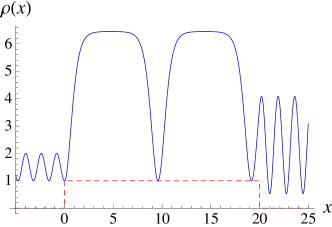
(a)

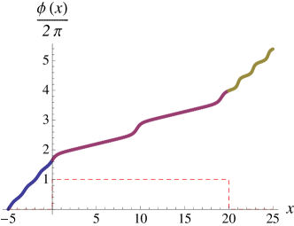
(b)

Figure 1: (Color online) Density (upper panel) and phase (lower panel) of a solution to the NLSE in which an incident near-sinusoidal wave produces a single dark soliton localized over the barrier. The density notch of a second dark soliton is formed near the far right of the barrier, around $x=19$, and a longer barrier could trap two or more dark solitons in a dark soliton train. The three colors in the phase curve denote the three scattering regions. The red dashed curve shows the potential barrier for reference.

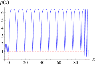
(a)

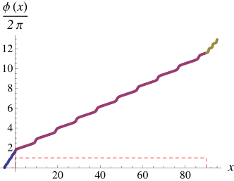
(b)

Figure 2: (Color online) Density (upper panel) and phase (lower panel), similar to Fig. 1, but with a soliton train localized on the barrier instead of a single soliton. The input parameters are identical to those of Fig. 1; only the barrier width has been changed, from 20 to 90. We observe a train of 9 very deep solitons localized on the barrier.

A large variety of solution types appear after following the methods of Sec. II. We present here some particularly interesting cases which are very far from the kinds of solutions found for the linear Schrödinger equation. We recall that, in the linear Schrödinger equation, the wavelength of the plane wave components across regions I, II, and III is the same; it is only the spatial offset in the arguments of the exponentials and the amplitudes that can be different. In the nonlinear case the wavelength can be quite different in all three regions. We present two such cases, in which a phonon-like standing wave is transformed into a strongly localized soliton or soliton train over the barrier, and then returns to a phonon-like profile. We recall that phonons are a limit of Bogoliubov quasi-particles for BECs, and appear as a small modulation on top of a large offset, qualitatively speaking, as ripples on a pond. Since we work with the fully nonlinear problem our phonons are not constrained to be small oscillations, but continue to appear as ripples of amplitude $A$ and translational offset $\delta_{0}$ on top of an offset of magnitude $B$.

Figure 1 shows the density and phase for a localized soliton. A well-localized solution can be seen above the potential barrier. The barrier, indicated with a red dashed box in the figure, has height $V_{0}=1$ and width 20. The nonlinearity is $g=2.02$ and the chemical potential $\mu=2.404$. We choose $A_{I}=1$, $B_{I}=1$, and $\delta_{0I}=0$. In regions I and III, outside the barrier, the elliptic parameter $m\ll 1$. In region II, over the barrier, $m$ approaches unity and the peaks of the $\text{sn}^{2}$ function broaden significantly. The local minimum of the density over the barrier is a dark soliton, called “grey” because it does not have a node. Such a soliton is always moving. Examining the phase profile, we observe two areas in region II: away from the dark soliton is a background superflow with a shallower slope, while over the soliton there is a characteristic phase jump displaying a sharp increase in slope. In this solution the superflow flows to the right with velocity $v=\partial_{x}\phi(x)$, while the dark soliton moves to the left with an equal and opposite velocity; the two velocities cancel each other, leading to a stationary state.

The phase has an overall linear envelope on either side of the barrier, with clearly visible oscillations on this background. The background slopes differ slightly between regions I and III, and the slope over the barrier in region II is smaller by a factor of 3. This shows that the velocity profile of the BEC need not be the same on either side of the barrier. Although we fixed parameters on the left-hand side in order to find this solution, as described in Sec. II, from the physical perspective of an atom laser the BEC is incident on the right-hand side. Thus, as happens approximately half the time in our solution method, we have in fact fixed the output rather than the input parameters. The overall transmission right to left is about 50%, and $T>1$ according to our definition from Eq. (23).

With a longer barrier of width $x_{2}-x_{1}=90$ and the same nonlinearity $g=2.02$, chemical potential $\mu=2.404$, and input parameters $A_{I}=1$, $B_{I}=1$, and $\delta_{0I}=0$ fixed on the left hand side, we obtain a soliton train localized on the barrier, as shown in Fig. 2. In Fig. 2 we again display the potential with a dashed red line for reference. The location of the dark solitons can be observed in both the density and the phase, similar to Fig. 1. Multiple solitons have been observed in a variety of BEC experiments strecker2002 ; engelsP2007 ; weller2008 . However, such solitons have so far not been phase-locked into a train in BECs. Our barrier method constitutes a totally new way of producing multiple solitons locked into a train. The length of the barrier can be used to control the number of solitons in the train. We note that dark soliton trains have been produced in nonlinear spin waves in thin magnetic films kalinikos2000 ; wuMingzhong2004 , but not via our scattering technique; also spin waves are in fact a damped driven system which are best modeled by an open-system version of the NLSE quite different from Eq. (9) carr2010g .

IV Atom Laser Transmission

We turn now to a more systematic exploration of the solution space. The nonlinear Schrödinger equation has a substantially larger parameter space to explore than the linear case. We divide this exploration into wide and narrow barriers. The barrier size $x_{2}-x_{1}$ can be compared to the BEC healing length, $\xi\equiv 1/\sqrt{8\pi\langle\rho\rangle a_{s}}$, with $\langle\rho\rangle$ the average linear number density. However, the healing length only provides a useful comparison for low-energy excitations, as it describes how a uniform ground-state BEC is perturbed by a localized potential, e.g. a hard wall. This corresponds to well-separated dark solitons, as in region II in Figs. 1 and 2. As we treat a wide variety of excitations, many of which take standing-wave form which is very far from the ground state, e.g. regions I and III in Figs. 1 and 2, the correct comparison to identify wide and narrow barriers is in fact the wavelength of the excitations,

$$\lambda\equiv\frac{2K(m)}{b}=\frac{2K\left(\frac{Ag}{2(\mu-V_{0})-(A+3B)g}\right)}{\sqrt{2(\mu-V_{0})-(A+3B)g}},$$ (29)

as can be calculated from Eqs. (12) and (10). Thus $x_{2}-x_{1}\ll\lambda_{j}$ is the narrow barrier case and $x_{2}-x_{1}\gg\lambda_{j}$ is the wide barrier case, where the subscript $j\in\{I,II,III\}$ refers to the region. For sufficiently small $\lambda$ all barriers are effectively wide. Holding other parameters fixed, including the nonlinearity, the wide barrier limit occurs for large chemical potential, since the wavelength is a decreasing function of $\mu$, as can be verified by consideration of Eq. (29).

We found that the barrier height $V_{0}$ is less important, a statement which we will support further in Sec. V. This dependence on width more than height is another sense in which the nonlinear case is very different from the linear case; in the latter it is only the effective area of the barrier, $2M\tilde{V}_{0}(\tilde{x}_{2}-\tilde{x}_{1})^{2}/\hbar^{2}$, that is important. The dependence on width arises mainly from the fact that the density in the nonlinear case can have different wavelengths in different regions for the same solution, in contrast to the linear case, as previously mentioned.

For simplicity we will keep the input parameters $A_{I}$, $B_{I}$, and $\delta_{0I}$ fixed to the same values as those used in Figs. 1-2 and Sec. III; after a massive exploration of the parameter space, we found all results to be qualitatively similar to those described below.

IV.1 Wide Barrier Case

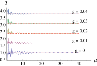
Figure 3: (Color online) Wide barrier, small nonlinearity. Transmission for wide barrier with increasing nonlinearity from bottom to top, starting with the linear case, $g=0$, in steps of $\Delta g=0.01$. Even a very small nonlinearity changes the problem because the left-right symmetry of the effective potential is broken.

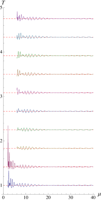
Figure 4: (Color online) Wide barrier, medium nonlinearity. Same as Fig. 3, but with steps of $\Delta g=0.1$, from $g=0.1$ to $g=1.0$ An extended region of near-perfect invisibility of the barrier in the $\mu\simeq 20$ to $\mu\simeq 30$ range translates to the right as the nonlinearity increases.

We consider a barrier whose width is much larger than its height. We take a barrier of width $x_{2}-x_{1}=20$ and height $V_{0}=1$ for the purposes of illustration. In Figs. 3-4 transmission plots are laid out on the same set of horizontal axes. The dashed red lines denote $T=1$, and solid curves are the transmission coefficient as defined in Eq. (23). The nonlinearity $g$ increases in steps of 0.01 in Fig. 4 as we move upward on the plot, and in steps of 0.1 in 3. Each transmission plot is at a convenient vertical offset for illustration, but the plots are not otherwise scaled or shifted. The nonlinearity is shown next to each curve for reference. As discussed in Section II.3, the transmission coefficient may be greater than 1. This is not a novel physical feature; it arises due to the redefinition of transmission as in Eq. (23) and the invalidity of superposition in this problem.

Comparing the linear, i.e $g=0$, transmission curve in Fig. 3 with the other transmission plots in the same figure, we observe that there is a significant change in transmission behavior when we enter the nonlinear regime, even for very small nonlinearity, $g\sim\mathcal{O}(10^{-2})$. The most significant change occurs when $\mu$ is small, meaning that the potential barrier has a greater overall effect on the condensate. In the linear case, $T$ oscillates about evenly on either side of unity for small $\mu$, and the amplitude of oscillations is similar in either direction. In the nonlinear case, we see that while transmission can still be less than unity, it does not drop as far below unity as in the linear case. We understand this difference to be due to the effective potential: for $g=0$ the operator in the NLSE is not biased, whereas for non-zero $g$ it is. Thus, by choosing parameters on the left hand side, we fix the effective potential and bias the system towards particular parameter sets.

As $g$ increases, new peaks appear in the small-$\mu$ regime, and the behavior of $T$ changes significantly for smaller $\mu$. This regime does not appear for $g\gtrsim 0.2$. The reason that the transmission curves depend strongly on $g$ in the small-$\mu$ regime is that $g$ and $\mu$ are not completely independent. For a given chemical potential $\mu$, when the nonlinearity $g$ becomes larger than a certain cut-off value, solutions are generated that have $\rho(x)\in\mathbb{C}$. This is invalid because, when we solved the NLSE, we assumed $\rho(x)\in\mathbb{R}$. We may take $\rho(x)\in\mathbb{R}$ without loss of generality, since Eq. (8) is a general polar representation of a complex number. For large $\mu$ the cut-off in $g$ is pushed to a region off the top of our plot; see figures in Sec. V for more details. The appearance of complex $\rho(x)$ means that one or more of our assumptions are breaking down in this regime. A more detailed analysis of this situation is considered in RRMthesis . One such break-down is due to the appearance of quasi-bound states with complex $\mu$ carr2004b ; carr2005c ; dekel2009 .

For larger values of $\mu$, the overall behavior of the transmission does not change significantly between each plot. However, we do see a shift in the transmission curve. For higher $\mu$, the transmission plot retains its shape and shifts to the right as $g$ increases. This feature is especially apparent when a computer is used to animate the transmission plots for increasing $g$; in Fig. 4 we have endeavored to lay such an animation out on the page. In Fig. 4, the regime of the same curve-shape translating gradually to the right with increasing $g$ occurs when $\mu\gtrsim 6$.

Another feature of note is that with the definition (23) of transmission, the amplitude of oscillations in $T$ does not decrease monotonically as in the usual linear interpretation. In all of the transmission plots of Fig. 4, we see significant oscillations on either side of a transition region between $\mu\simeq 20$ and $\mu\simeq 30$. In this region, we have almost perfect resonance, i.e., $T$ is very close to unity. Further analysis of transmission resonances will be presented in Sec. V.

IV.2 Narrow barrier

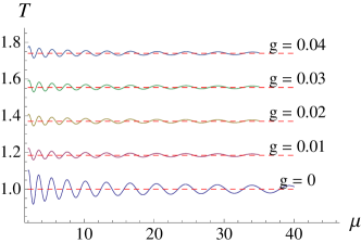
Figure 5: Transmission for narrow barrier with small nonlinearity. Note the difference in behavior between the linear and nonlinear regimes.

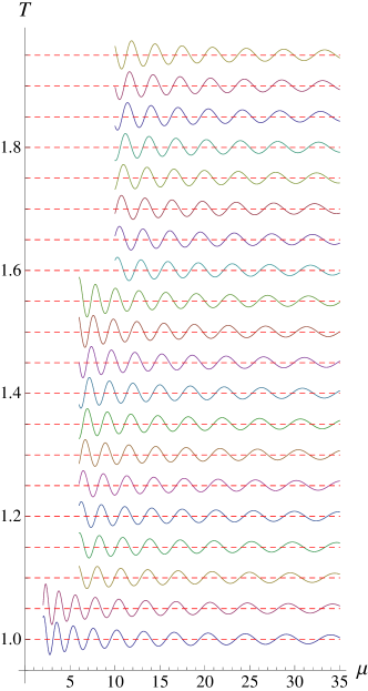
Figure 6: Transmission for narrow barrier with increasing nonlinearity from bottom to top, from $g=0.1$ to $g=2.0$ in steps of $\Delta g=0.1$.

To explore the narrow-barrier regime, we choose $x_{2}-x_{1}=0.1$ and $V_{0}=10$, so that the barrier is a factor of ten narrower than it is high; note that the height is the same as the wide-barrier case explored in Sec. IV.1. Over the full range of values of $\mu$ and $g$ that we consider, the narrow-barrier requirement, $\lambda\gg x_{x}-x_{1}$, is satisfied, as can be verified from Eq. (13); in the range we consider, $\lambda\geq 0.35$. We first focus on transmission plots for small nonlinearity, in Fig. 5. The layout of the figure is the same as in Sec. IV.1: five transmission plots are shown on the same set of horizontal axes, with vertical offsets in $T$ for illustration, the plots are not otherwise shifted or scaled, and $g$ is increased from zero in steps of $\Delta g=0.01$. Comparing the linear $g=0$ transmission curve with those for $g>0$, we again see a significant drop in the amplitude of oscillations as we go from the linear to the nonlinear regime. Again, the nonlinear transmission curves tend to stay further above unity than below unity, although the difference is less pronounced than in the wide-barrier case. As a function of $\mu$ the transmission curve is much smoother as compared to Fig. 3. This is because there is always less than one wavelength fitting into the barrier, and thus a small change in $\mu$ cannot suddenly cause an integer number of wavelengths to match the barrier width.

In Fig. 6, we turn to the regime of medium nonlinearity, increasing $g$ from 0.1 in steps of $\Delta g=0.1$ up to $g=2.0$. The amplitude of oscillations decreases smoothly for increasing $\mu$, independent of $g$. There is no region of near-perfect resonance as in the wide-barrier case: $T$ oscillates quasi-periodically about $T=1$. In fact, the entire transmission curve simply translates smoothly to the right as $g$ increases, with no real abrupt behavior even for the smallest values of $\mu$ allowed for each curve. Thus we can surmise that the abrupt behavior in Sec. IV.1 is due to the barrier width, and it is the width, not the height, that mainly controls the transmission curves. In the following section we will adduce further evidence to support this point.

V Transmission Resonances and Bifurcations

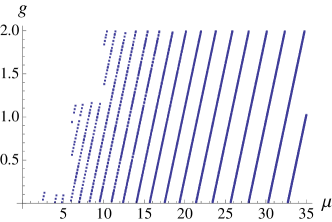
Figure 7: Transmission resonances for narrow barrier. All behavior is described by regularly spaced straight lines except for very small $\mu$, where some combinations of $g$ and $\mu$ do not produce stationary solutions.

To better understand the results of Sec. IV, in particular the extended region of near-perfect invisibility of the barrier, we focus on the transmission resonances only, i.e., the points in the $g$–$\mu$ plane for which $T=1$ to within a tolerance of $10^{-5}$.

We first treat the simpler case of the narrow barrier. The transmission resonances from Fig. 6 are shown in Fig. 7. This clearly shows that all transmission resonances translate smoothly to the right for increasing $g$, with a constant slope. This figure allows us to predict the location of all transmission resonances except for small $\mu$, where constraints in the allowed simultaneous values of $g$ and $\mu$ cut off certain regions, as discussed in Sec. IV. We also observe in Fig. 7 that the spacing between curves increases with increasing $\mu$. A functional fit to this spacing can allow us to predict transmission resonances in the entire $g$–$\mu$ plane. Since the spacing is the same starting from $g=0$, it is straightforward to find such a function for any values of $A$, $B$, and $\delta_{0}$.

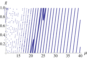
Figure 8: Transmission resonances for wide barrier. Bifurcations occur in an extended region of near-perfect invisibility of the barrier.

With the narrow-barrier case as a reference, we move on to the more intricate wide-barrier case. Figure 8 shows the transmission resonances from Fig. 4. We observe that the resonances are sparse for low values of $\mu$, with much more sporadic and abrupt behavior than the narrow barrier case. This is because an integer number of wavelengths can fit into the barrier width, an effect which is more pronounced for small $\mu$; for instance, for $g=0.02$ and $\mu=2$, $\lambda=2.27$, while for $\mu=40$, $\lambda=0.355$. In the regions where lines of resonance appear, the spacing between these lines is smaller than in Fig. 7. The spacing increases as $\mu$ increases, though not as fast as in the narrow-barrier case.

The resonances are sparse for lower values of $\mu$ and more uniform for higher values of $\mu$. For mid-range $\mu$, we see very different behavior. There are three regions between $\mu=20$ and $\mu=26$ where the resonances are extremely dense. These correspond to the region of near-constant resonance seen in the transmission plots. This region shifts to the right as $g$ increases, as observed in the transmission plots. Three bifurcations are present in this region. Bifurcations are typical of nonlinear systems; the particular example we show here for this parameter set is expected to be a generic feature for all parameter sets. Further numerical exploration found these three bifurcations continued in an apparently infinite sequence sloping away upwards to the right. We found that a linear function was not sufficient to fit such bifurcations, and they occurred near but not precisely at a value of $\lambda=1/2$. We did not find bifurcations at other rational values of $\lambda$, so this may be a coincidence; the barrier length in this parameter set is $x_{2}-x_{1}=10$. We explored up to $\mu=70$ and $g=10$. Although our computationally intensive study was only performed thoroughly for this particular choice of parameters, we did spot checks through many regions of parameter space and observed similar extended regions of near-perfect invisibility of the barrier.

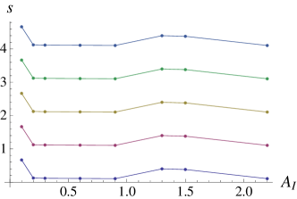
Figure 9: Slopes of resonance transmission lines, as a function of density offset, coarse sampling. The curves show $B=0.2$, 0.5, 1.0, 1.5, 2.0 from bottom to top; a vertical offset is given to each curve for visualization, since they in fact all lie on top of each other. The points represent actual data, while the curves are a guide to the eye.

We return to the narrow barrier case for further analysis. We consider the slope $s$ of these parallel lines of resonance as a function of other physical parameters. For the parameter regimes considered in this study, the slope of the resonance lines does not depend on the value of the density offset, $B$, as seen in Fig. 9. In this plot, the slope is shown for several values of $B$. Each curve has been vertically shifted by a convenient offset for illustration; all curves in fact lie on top of each other. We note that the elliptic parameter $m$, which is strongly governed by the nonlinearity of the system, depends on both $A$ and $b$, but does not depend on $B$, as described in Sec. II.2. Similarly, we found that the slopes $s$ do not depend on the spatial translational offset $\delta_{0}$. However, the slopes do depend strong on the amplitude $A$. The slope decreases as the amplitude of the input density increases. We find an exponential least-squares fit as shown in Fig. 10:

$$s(A_{I})=0.167+0.485e^{-0.549A_{I}},$$ (30)

where we fixed $B_{I}=1.0$.

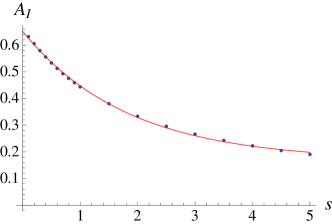
Figure 10: Slope of resonance curves as a function of input amplitude. Although the transmission resonances curves do not depend on $B$ and $\delta_{0}$, they do depend strongly on $A$. Points are numerical calculations, while the solid curve is a least squares fit.

VI Conclusions

We developed a general method for obtaining stationary states of the nonlinear Schrödinger equation for any piecewise constant potential. We applied this method to nonlinear scattering on a rectangular potential barrier, focusing on cnoidal waves, or dark soliton trains. This problem differs greatly from the textbook linear quantum mechanics problem of scattering on a rectangular barrier. Among novel nonlinear features are the following. First, the wavelength in the three regions (left of the barrier, on the barrier, and right of the barrier) need not be the same. As a consequence, such a barrier can be used to create one or more sharply localized dark solitons from a broad phonon-like input. Second, it is mainly the barrier width, not its area, that controls the kind of stationary states observed. For wide barriers in which the barrier width is larger than the wavelength extended regions of near-perfect transmission occur; the barrier is invisible over a range of interaction strength $g$ and chemical potential $\mu$. Third, in wide barriers an apparently infinite sequence of bifurcations appears in this invisibility region. Despite the parameter space for solutions being large, we showed that it is just the amplitude that determines slopes of transmission resonance lines, greatly simplifying this complex problem.

To relate our predictions to alternate physical input of average density, momentum, and energy of an atom laser formed from a Bose-Einstein condensate, the analysis laid out in Ref. carr2005a may be used directly; thus we do not repeat it here. Future possibilities for this work include applying our method to various piecewise constant potentials of interest in applications, and a more detailed mathematical study of the bifurcations we found in transmission resonances.

We acknowledge helpful discussions with Paul A. Martin and Matthew Heller. This material is based in part upon work supported by the National Science Foundation under Grant Numbers PHY-0547845 and PHY-1067973. L.D.C. thanks the Alexander von Humboldt foundation for additional support, and the Institute for Advanced Study at Tsinghua University for hosting him during completion of a significant portion of this work.

Appendix A Jacobi Elliptic Functions

There are twelve Jacobi elliptic functions in all: sn, cn, dn, sc, nc, dc, cs, ds, ns abramowitz1964 . Not all of these are independent. The Jacobi functions are doubly-periodic in the complex plane and they depend on two parameters: an independent variable $u$ and the elliptic parameter $m$. For real parameter $m$, we may assume $0\leq m\leq 1$. If $m$ is outside of this range, transformations can be made to write the Jacobi function in terms of functions whose parameter is between 0 and 1. For $\text{sn}\,(u|m)$, which appears in the density $\rho(x)$ of the BEC, these transformations are, for $m<0$,

$$\text{sn}\,(u|m) = \left(\frac{1}{1-m}\right)^{1/2}$$ (31)

$$\times\,\text{sd}\left[(1-m)^{1/2}u\bigg{|}\left(\frac{-m}{1-m}\right)\right],$$

and for $m>1$,

$$\text{sn}\,(u|m)=m^{-1/2}\text{sn}\,(um^{1/2}|m^{-1}).$$ (32)

When $m$ lies between zero and unity, the Jacobi functions can be interpreted geometrically as the analog of the hyperbolic and trigonometric functions. In this interpretation, the parameter $m$ corresponds to the eccentricity of the ellipse. For $m=0$, the Jacobi functions reduce to the trigonometric functions; for $m=1$, to the hyperbolic functions.

The Jacobi elliptic functions are defined as inverse integrals bowman1 , and by the locations of zeros and poles in the complex plane abramowitz1964 . They may be related to one another by various identities fettis1972 ; khare2002 ; dayton2002 .

Appendix B Proofs

B.1 Linear Independence of Powers of $\bm{\text{sn}\,(u|m)}$

In the following we state a particularly vital proof which we have not found elsewhere in the literature, and is required to establish our exact solutions. Other proofs can found in Ref. RRMthesis .

Theorem B.1.

The functions $\text{sn}^{p}(u|m)$ and $\text{sn}^{q}(u|m),~{}p,q\in\mathbb{Z}$, are linearly independent for $p\neq q$.

Proof.

Compute the Wronskian of the two functions:

$$W[\text{sn}^{p}(u|m),\text{sn}^{q}(u|m)]=$$

$$\qquad\qquad\begin{vmatrix}\text{sn}^{p}(u|m)&\text{sn}^{q}(u|m)\\ \frac{\partial}{\partial u}[\text{sn}^{p}(u|m)]&\frac{\partial}{\partial u}[\text{sn}^{q}(u|m)]\end{vmatrix}$$ (33)

$$=q\text{sn}^{p}(u|m)\text{sn}^{q-1}(u|m)\text{cn}\,(u|m)\text{dn}\,(u|m)$$

$$\qquad-p\text{sn}^{p-1}(u|m)\text{sn}^{q}(u|m)\text{cn}\,(u|m)\text{dn}\,(u|m)$$ (34)

$$=(q-p)\text{cn}\,(u|m)\text{dn}\,(u|m)\text{sn}^{p+q-1}(u|m).$$ (35)

The product of Jacobi elliptic functions is nonvanishing except on a set of measure zero; therefore, for $p\neq q$ the functions are linearly independent. QED.

B.2 Linear Independence of Products of Powers of $\bm{\text{sn}\,(u|m)}$

Let

$$f_{1}(x)=\text{sn}^{p}(a|m)\text{sn}^{q}(u|m),$$ (36)

$$f_{2}(x)=\text{sn}^{r}(a|m)\text{sn}^{s}(u|m),$$ (37)

where $p$, $q$, $r$, $s$ are integers, and $a$ and $u$ are linear functions of $x$. We may assume without loss of generality that $a\neq u$. The case $a=u$ is analyzed in Section B.1. Computing the Wronskian of $f_{1},f_{2}$, we find

$$W(f_{1},f_{2})=\\ (r-p)\text{cn}\,(a|m)\text{dn}\,(a|m)\text{sn}^{r+p-1}(a|m)\text{sn}^{s+q}(u|m)+\\ (q-s)\text{cn}\,(u|m)\text{dn}\,(u|m)\text{sn}^{s+q-1}(u|m)\text{sn}^{r+p}(a|m).$$ (38)

The Wronskian vanishes $\forall a,u$ only when $r=p$ and $q=s$; that is, when $f_{1}$ and $f_{2}$ are not distinct functions. In all other cases, $f_{1}$ and $f_{2}$ are linearly independent.

Appendix C Numerical Convergence

We consider several limits of the NLSE, Eq. (9). These are used to verify consistency of our code with known results.

C.1 Linear Limit

We consider the NLSE, Eq. (9), in the limit that $g\to 0$. In this limit, the solution should reduce to the well-known linear scattering solution, which is analyzed in many elementary quantum mechanics texts. In the linear limit, we find that $m\to 0$, so that the linear density is

$$\rho(x)=A\sin^{2}(bx+\delta_{0}),$$ (39)

since $B=0$ in the linear case RRMthesis . For comparison with the nonlinear case, we define transmission as $\langle\rho_{III}\rangle/\langle\rho_{I}\rangle$. The integral for $\langle\rho\rangle$ can be evaluated exactly in this case:

$$\langle\rho\rangle =\int_{0}^{2\pi/b}\!dx\,A\sin^{2}(bx+\delta_{0})\,,$$ (40)

$$=\tfrac{1}{2}A.$$ (41)

Therefore, the transmission is

$$T_{\ell}=\frac{A_{III}}{A_{I}}.$$ (42)

We can compare the value given by Eq. (42) to the value $T$ obtained numerically by the code. Transmission plots are shown in Figs. 11a and 11b. A log plot of the error,

$$\varepsilon=\frac{|T-T_{\ell}|}{T_{\text{avg}}},$$ (43)

is given in Fig. 11c. The maximum value of the error is $\mathcal{O}(10^{-7})$, which is within the numerical tolerance of the code.

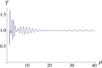
(a)

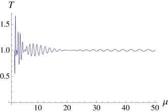
(b)

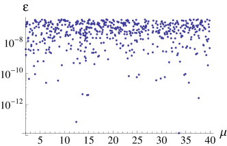
(c)

Figure 11: (a) Numerically computed transmission for linear limit. (b) Exact linear value of transmission. (c) Error in transmission for linear limit.

C.2 Constant Potential Limit

Consider the NLSE, Eq. (9), with potential barrier (15), in the limit that $V_{0}\to 0$. In this case, boundary conditions are redundant and we expect all parameters to be constant $\forall x$. By setting a “barrier” of $V_{0}=0$ in the code, we can verify that the code gives the correct solution; namely, the amplitude, period, and shifts in the density should not change at the “boundary” locations. Indeed this is the case, providing an additional verification of correctness for the code. A density plot for this case, with a “barrier” of width 5 and height 1, is shown in Fig. 12.

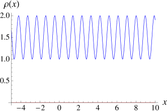
Figure 12: Density plot for zero barrier.

Since the density parameters do not change over space, we expect to find a transmission coefficient of 1. We compute and plot the error

$$\varepsilon=\ln\left(\frac{|T-1|}{T_{\text{avg}}}\right),$$ (44)

where $T_{\text{avg}}$ denotes the average value of transmission over the plot interval. A log plot of the error is given in Fig. 13.

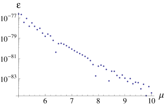
Figure 13: Error in transmission for zero barrier.

Alternatively, we can consider a constant nonzero potential: $V(x)=V_{c},~{}\forall x$ in Eq. (9). Again we expect all parameters to be constant $\forall x$. We set a “barrier” of $V_{I}=V_{II}=V_{III}=2$ and width 5 in the code and plot the density. The plot is shown in Fig. 14.

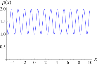
Figure 14: Density plot for nonzero flat barrier.

Again, since the density parameters do not change over space, we expect to find a transmission coefficient of 1. We compute and plot the error

$$\varepsilon=\ln\left(\frac{|T-1|}{T_{\text{avg}}}\right),$$ (45)

where $T_{\text{avg}}$ denotes the average value of transmission over the plot interval. A log plot of the error is given in Fig. 15.

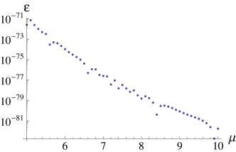
Figure 15: Error in transmission for nonzero flat barrier.

Therefore the code gives the expected results for density and transmission in the constant-potential limits.

C.3 Thomas-Fermi Limit

We consider the limit that $\hbar\partial^{2}\Psi/\partial x^{2}\to 0$ in the unscaled NLSE, Eq. (1). In this limit, the unscaled NLSE becomes

$$\left[g|\Psi(x,t)|^{2}+V(x)\right]\Psi(x,t)=i\hbar\frac{\partial}{\partial t}\Psi(x,t).$$ (46)

Substituting Eq. (8) for the wave function $\Psi$ in (46) and rearranging, we obtain

$$g\rho^{3/2}+[V(x)-\hbar\mu]\rho^{1/2}=0,$$ (47)

so that either $\rho(x)\equiv 0$, the trivial case, or else

$$\rho(x)=[\hbar\mu-V(x)]/g,$$ (48)

when $g\neq 0$. Note that Eq. (48) works for any spatially-dependent potential $V(x)$.

Equation (48) is the well-known Thomas-Fermi limit dalfovo1999 . It is relevant when the curvature of $\Psi$ is nearly zero. This can be accomplished either by taking the limit $A/B\to 0$, so that the amplitude of oscillations is small, or by taking the limit $1/b\to\infty$, so that the wavelength of oscillations is large.

References

- (1) F. Dalfovo, S. Giorgini, L. P. Pitaevskii, and S. Stringari, Rev. Mod. Phys. 71, 463 (1999).
- (2) W. Ketterle, D. S. Durfee, and D. M. Stamper-Kurn, in Proceedings of the International School of Physics “Enrico Fermi” (IOS Press, Amsterdam; Washington, D.C., 1999), pp. 67–176.
- (3) B. P. Anderson and M. A. Kasevich, Science 282, 1686 (1998).
- (4) E. W. Hagley, L. Deng, M. Kozuma, J. Wen, K. Helemerson, S. L. Rolston, and W. D. Phillips, Science 283, 1706 (1999).
- (5) I. Bloch, T. W. Hänsch, and T. Esslinger, Phys. Rev. Lett. 82, 3008 (1999).
- (6) O. Zobay, E. V. Goldstein, and P. Meystre, Phys. Rev. A 60, 3999 (1999).
- (7) K. Helmerson, D. Hutchinson, K. Burnett, and W. D. Phillips, Phys. World 12, 31 (1999).
- (8) P. Engels and C. Atherton, Phys. Rev. Lett. 99, 160405 (2007).
- (9) D. Dries, S. E. Pollack, J. M. Hitchcock, and R. G. Hulet, e-print arXiv:1004.1891 (2010).
- (10) V. Hakim, Phys. Rev. E 55, 2835 (1997).
- (11) N. Pavloff, Phys. Rev. A 66, 013610 (2002).
- (12) B. T. Seaman, L. D. Carr, and M. J. Holland, Phys. Rev. A 71, 033609 (2005).
- (13) D. Witthaut, S. Mossmann, and H. J. Korsch, J. Phys. A: Math. Gen. 38, 1777 (2005).
- (14) B. T. Seaman, L. D. Carr, and M. J. Holland, Phys. Rev. A 71, 033622 (2005).
- (15) T. Paul, P. Schlagheck, P. Leboeuf, and N. Pavloff, Phys. Rev. Lett. 98, 210602 (2007).
- (16) The results of our study can be qualitatively applied to a barrier of smooth shape with the same area as the rectangular barrier.
- (17) M. Olshanii, Phys. Rev. Lett. 81, 938 (1998).
- (18) D. S. Petrov, G. V. Shlyapnikov, and J. T. M. Walraven, Phys. Rev. Lett. 85, 3745 (2000).
- (19) L. D. Carr, M. A. Leung, and W. P. Reinhardt, J. Phys. B: At. Mol. Opt. Phys. 33, 3983 (2000).
- (20) V. Dunjko, V. Lorent, and M. Olshanii, Phys. Rev. Lett. 86, 5413 (2001).
- (21) Emergent Nonlinear Phenomena in Bose-Einstein Condensates, edited by P. G. Kevrekidis, D. J. Frantzeskakis, and R. Carretero-González (Springer-Verlag, Berlin, 2008).
- (22) L. D. Carr, C. W. Clark, and W. P. Reinhardt, Phys. Rev. A 62, 063610 (2000).
- (23) L. D. Carr, C. W. Clark, and W. P. Reinhardt, Phys. Rev. A 62, 063611 (2000).
- (24) B. T. Seaman, L. D. Carr, and M. J. Holland, Phys. Rev. A 72, 033602 (2005).
- (25) L. D. Carr, K. W. Mahmud, and W. P. Reinhardt, Phys. Rev. A 64, 033603 (2001).
- (26) K. Rapedius, D. Witthaut, and H. J. Korsch, Phys. Rev. A 73, 033608 (2006).
- (27) H. A. Ishkhanyan and V. P. Krainov, Phys. Rev. A 80, 045601 (2009).
- (28) T. Ernst and J. Brand, Phys. Rev. A 81, 033614 (2010).
- (29) C. Weiss and Y. Castin, Phys. Rev. Lett. 102, 010403 (2009).
- (30) A. I. Streltsov, O. E. Alon, and L. S. Cederbaum, Phys. Rev. A 80, 043616 (2009).
- (31) J. Denschlag, J. E. Simsarian, D. L. Feder, C. W. Clark, L. A. Collins, J. Cubizolles, L. Deng, E. W. Hagley, K. Helmerson, W. P. Reinhardt, S. L. Rolston, B. I. Schneider, and W. D. Phillips, Science 287, 97 (2000).
- (32) A. Weller, J. P. Ronzheimer, C. Gross, J. Esteve, M. K. Oberthaler, D. J. Frantzeskakis, G. Theocharis, and P. G. Kevrekidis, Phys. Rev. Lett. 101, 130401 (2008).
- (33) S. Burger, K. Bongs, S. Dettmer, W. Ertmer, K. Sengstock, A. Sanpera, G. V. Shlyapnikov, and M. Lewenstein, Phys. Rev. Lett. 83, 5198 (1999).
- (34) L. Khaykovich, F. Schreck, F. Ferrari, T. Bourdel, J. Cubizolles, L. D. Carr, Y. Castin, and C. Salomon, Science 296, 1290 (2002).
- (35) W. P. Reinhardt and C. W. Clark, J. Phys. B: At. Mol. Opt. Phys. 30, L785 (1997).
- (36) S. Stellmer, C. Becker, P. Soltan-Panahi, E.-M. Richter, S. Dörscher, M. Baumert, J. Kronjäger, K. Bongs, and K. Sengstock, Phys. Rev. Lett. 101, 120406 (2008).
- (37) R. R. Miller, Master’s thesis, Colorado School of Mines, 2010.
- (38) Handbook of Mathematical Functions, edited by M. Abramowitz and I. A. Stegun (National Bureau of Standards, Washington, D. C., 1964).
- (39) The final condition, , is not strictly required when the density vanishes on the boundary; however, in the latter case, one can argue this condition holds on physical grounds RRMthesis .
- (40) T. Paul, M. Albert, P. Schlagheck, P. Leboeuf and N. Pavloff, Phys. Rev. A 80, 033615, (2009).
- (41) P. Leboeuf, N. Pavloff, and S. Sinha, Phys. Rev. A 68, 063608 (2003).
- (42) T. Paul, M. Hartung, K. Richter, and P. Schlagheck, Phys. Rev. A 76, 063605 (2007).
- (43) B. I. Ivlev and N. B. Kopnin, Adv. Phys. 33, 47 (1984).
- (44) J. S. Langer and V. Ambegaokar, Phys. Rev. 164, 498 (1967).
- (45) P. Leboeuf and N. Pavloff, Phys. Rev. A, 64, 033602 (2001).
- (46) W. H. Press, S. A. Teukolsky, W. T. Vetterling, and B. P. Flannery, Numerical Recipes in C: The Art of Scientific Computing (Cambridge Univ. Press, Cambridge, U.K., 1993).
- (47) K. E. Strecker, G. B. Partridge, A. G. Truscott, and R. G. Hulet, Nature 417, 150 (2002).
- (48) B. A. Kalinikos, M. M. Scott, and C. E. Patton, Phys. Rev. Lett. 84, 4697 (2000).
- (49) M. Wu, B. A. Kalinikos, and C. E. Patton, Phys. Rev. Lett. 93, 157207 (2004).
- (50) Z. Wang, A. Hagerstrom, J. Q. Anderson, W. Tong, M. Wu, L. D. Carr, R. Eykholt, and B. A. Kalinikos, Phys. Rev. Lett. 107 114102 (2011).
- (51) N. Moiseyev, L. D. Carr, B. A. Malomed, and Y. B. Band, J. Phys. B: At. Mol. Opt. Phys. 37, L1 (2004).
- (52) L. D. Carr, M. J. Holland, and B. A. Malomed, J. Phys. B: At. Mol. Opt. 38, 3217 (2005).
- (53) G. Dekel, V. Farberovich, V. Fleurov, and A. Soffer, arXiv e-print:0911.1537 (2009).
- (54) F. Bowman, Introduction to Elliptic Functions, with Applications (Dover, New York, 1961).
- (55) H. E. Fettis, Mathematics of Computation 26, 965 (1972).
- (56) A. Khare, A. Lakshminarayan, and U. Sukhatme, Pramana Journal of Physics 62, 1201 (2004).
- (57) B. Dayton, in Theory of Equations (Oakton, Des Plaines, IL, 2002), Chap. Analysis – Elliptic Functions.