Role of non-collective excitations in low-energy heavy-ion reactions

Abstract

We investigate the effect of single-particle excitations on heavy-ion reactions at energies near the Coulomb barrier. To this end, we describe single-particle degrees of freedom with the random matrix theory and solve the coupled-channels equations for one-dimensional systems. We find that the single-particle excitations hinder the penetrability at energies above the barrier, leading to a smeared barrier distribution. This indicates that the single-particle excitations provide a promising way to explain the difference in a quasi-elastic barrier distribution recently observed in ²⁰Ne + ^90,92Zr systems.

I Introduction

Heavy-ion reactions near the Coulomb barrier provide a good opportunity to investigate an interplay between the reaction process and internal excitations in the colliding nuclei. For example, it is well known that subbarrier fusion cross sections are significantly enhanced as compared to a prediction of a simple barrier penetration model because of the couplings of the relative motion between the colliding nuclei to nuclear intrinsic degrees of freedom dasgupta . It has been well recognized by now that the enhancement of fusion cross sections can be explained in terms of a distribution of Coulomb barrier heights originated from the couplings fusionbar . The barrier distribution can be actually extracted directly from the experimental data by taking the second derivative of the product of fusion cross section $\sigma_{\rm fus}$ and the center of mass energy $E$ with respect to $E$, that is, $d^{2}\left(E\sigma_{\rm fus}(E)\right)/dE^{2}$ fusionbar . The experimental data have clearly shown that the barrier distribution makes a useful representation to understand the reaction dynamics of heavy-ion subbarrier fusion reactions dasgupta ; fusionexp .

A similar concept of barrier distribution has been applied also to heavy-ion quasi-elastic scattering (that is, a sum of elastic, inelastic scattering, and transfer reactions) timmers ; qelbar . In this case, the barrier distribution is defined as the first derivative of the ratio of the quasi-elastic scattering cross section at a backward angle $\sigma_{\rm qel}$ to the Rutherford cross section $\sigma_{\rm R}$, that is, $-d\left(\sigma_{\rm qel}/\sigma_{\rm R}\right)/dE$. The fusion and quasi-elastic barrier distributions have been found to behave similarly to each other at least in a qualitative way timmers ; zamrun .

In order to analyse the subbarrier enhancement of fusion cross sections and fusion and quasi-elastic barrier distributions, the coupled-channels method has been successfully employed. Typically, a few low-lying collective excitations are taken into account in a calculationdasgupta ; ccfull . With this approach, the barrier distribution arises naturally through the eigen-channel representation dasgupta ; dasso2 ; HTB97 ; NBT86 .

Recently, however, a few experimental data which cannot be accounted for by the conventional coupled-channels calculation have been obtained NBD04 ; J02 ; D07 ; S08 ; piasecki . One of these examples is the quasi-elastic scattering experiment for the ${}^{20}{\rm Ne}+^{90,92}{\rm Zr}$ systems piasecki . The experimental data show that the quasi-elastic barrier distribution for these systems behaves in a significantly different way from each other: the barrier distribution for the ²⁰Ne+${}^{92}{\rm Zr}$ system is much more smeared than that for the ²⁰Ne+${}^{90}{\rm Zr}$ system piasecki . On the other hand, the coupled-channels calculations that take into account the collective rotational excitations in ²⁰Ne as well as the vibrational excitations in ^90,92Zr lead to similar barrier distributions for both systems, because the strongly deformed ${}^{20}{\rm Ne}$ nucleus mainly determines the barrier structure while the difference in the collective excitations in the two Zr targets plays a minor role. In Ref. piasecki , it was suggested that single-particle excitations in the colliding nuclei are responsible for smearing the barrier distribution for the ²⁰Ne + ⁹²Zr system. Notice that the single-particle excitations are expected to be much more important for the ${}^{92}{\rm Zr}$ nucleus compared to the ${}^{90}{\rm Zr}$ nucleus, which has the $N=50$ shell closure. In fact, while there are only 12 states in the ⁹⁰Zr nucleus up to 4 MeV, there are 53 known states in the ⁹²Zr nucleus bnl . For 5 MeV, the number of known states is 35 and 87 for ⁹⁰Zr and ⁹²Zr, respectively (for another nucleus, ¹¹⁶Sn, there are 81 known levels up to 3.9 MeV and 112 levels up to 4.3 MeV RWK91 ; IWRK93 ).

The aim of this paper is to investigate the effect of low-lying single-particle excitations on low-energy heavy-ion reactions, as conjectured in Ref. piasecki . In order to understand qualitatively the effect of non-collective excitations, in this paper we shall use a schematic model, that is, one-dimensional barrier penetration in the presence of the couplings to intrinsic degrees of freedom. The single-particle degrees of freedom can be described in several ways diaz ; akw1 ; akw2 ; akw3 ; akw4 ; zagrebaev . For instance, Ref.diaz used the Lindblad approach to discuss the role of quantum decoherence in deep subbarier hinderance of fusion cross sections. In this paper, we employ the random matrix theory (RMT) to describe the single-particle excitations (see Refs. PW07 ; rmtrev ; rmtrev2 ; B97 for recent reviews on RMT). The random matrix approach for heavy-ion reactions has been developed in 1970’s by Weidenmüller and his collaborators in order to analyse heavy-ion deep inelastic collisions (DIC) akw1 ; akw2 ; akw3 ; akw4 . At that time, they derived the transport coefficients based on RMT BNW79 and solved the classical transport equations (see also Refs. TNOY81 ; NT83 ). The RMT has also been employed to discuss quantum dissipation W90 ; BDK96 ; MA97 . In this paper, instead of solving the classical equations, we directly solve the coupled-channels equations quantum mechanically by including the single-particle excitations described by RMT. Our approach is therefore similar to that in Ref. zagrebaev , in which the coupled-channels equations with 200 dimension were solved for a one-dimensional model using a semi-classical approximation. In contrast to Ref. zagrebaev , we apply our formalism to the subbarrier regime without using the semi-classical approximation. This will enable us to assess the effect of single-particle excitations on quantum tunneling and thus on the barrier distribution. By treating the single-particle states explicitly, we can also discuss the excitation spectra as a function of incident energy.

The paper is organized as follows. In Sec. II, we detail the coupled-channels formalism with single-particle excitations described by RMT. In Sec. III, we apply the formalism to one-dimensional models for quantum tunneling. We discuss the effect of single-particle excitations on the barrier penetrability, the barrier distribution, and the excitation spectra. Using the results for the one-dimensional model, we also discuss the effect of non-collective excitations on quasi-elastic barrier distribution for the ²⁰Ne+⁹²Zr system. We then summarize the paper in Sec. IV.

II formalism

II.1 Coupled-channels method

The aim of this paper is to discuss the effect of single-particle excitations on one-dimensional barrier penetrability. For this purpose, we assume the following Hamiltonian:

$$H=-\frac{\hbar^{2}}{2\mu}\frac{d^{2}}{dx^{2}}+V_{\rm rel}(x)+H_{0}(\xi)+V_{\rm coup}(x,\xi).$$ (1)

Here, $\mu$ is the reduced mass and $V_{\rm rel}(x)$ is a potential for the relative motion. $H_{0}(\xi)$ is a Hamiltonian for the intrinsic degrees of freedom of the colliding nuclei, and the last term, $V_{\rm coup}(x,\xi)$, is a coupling Hamiltonian between the relative motion and the internal degrees of freedom.

The coupled-channels equations for this Hamiltonian are obtained by expanding the total wave function in terms of the eigen functions of $H_{0}(\xi)$ and read,

$$\left\{-\frac{\hbar^{2}}{2\mu}\frac{d^{2}}{dx^{2}}+V_{\rm rel}(x)+\epsilon_{n}-E\right\}\psi_{n}(x)$$

$$+\sum_{m}V_{nm}(x)\psi_{m}(x) = 0.$$ (2)

Here, $\epsilon_{n}$ and $\psi_{n}(x)$ are the excitation energy and the wave function for the $n$-th channel, respectively. $V_{nm}(x)$ is a coupling matrix and is a function of the coordinate $x$.

The coupled-channels equations are solved by imposing the boundary conditions of

$$\psi_{n}(x) \rightarrow\delta_{n,0}\,e^{-ik_{0}x}+r_{n}\,e^{ik_{n}x}\ \ \ {\rm for}\ \ \ x\rightarrow+\infty$$ (3)

$$\rightarrow t_{n}\,e^{-ik_{n}x}\ \ \ {\rm for}\ \ \ x\rightarrow-\infty,$$ (4)

where $\displaystyle k_{n}=\sqrt{{2\mu(E-\epsilon_{n})}/{\hbar^{2}}}$ is the wave number for the $n$-th channel, and 0 represents the entrance channel. We have assumed that the projectile is incident from the right hand side of the potential barrier. With the transmission coefficients $t_{n}$, the penetration probability for the inclusive process is calculated as

$$P(E)=\sum_{n}P_{n}(E)=\sum_{n}\frac{k_{n}}{k_{0}}|t_{n}|^{2}.$$ (5)

The barrier distribution is obtained by taking the derivative of $P(E)$, that is, $dP(E)/dE$ HTB97 .

In order to take into account the single-particle excitations, as we will show in the next section, one has to include a large number of channels. Since it is time and memory consuming to solve the coupled-channels equations with a large dimensionality, in this paper we employ a constant coupling approximation dasso2 . In this approximation, the coupling matrix is assumed to be a constant over the whole range of $x$. Then, one can diagonalize the matrix $A=(V_{nm}+\epsilon_{n}\delta_{n,m})$ with a coordinate independent unitary matrix $U$,

$$UAU^{\dagger}=diag\left\{\lambda_{1},\lambda_{2},\cdots\right\}$$ (6)

where, $\lambda_{1},\lambda_{2},\cdots$ are the eigenvalues of $A$. Transforming the channel wave functions as

$$\widetilde{\psi}_{n}(x)=\sum_{m}U_{nm}\psi_{m}(x),$$ (7)

the coupled-channels equations are transformed to a set of the uncoupled equations,

$$\left\{-\frac{\hbar^{2}}{2\mu}\frac{d^{2}}{dx^{2}}+V_{\rm rel}(x)+\lambda_{n}-E\right\}\widetilde{\psi}_{n}(x)=0.$$ (8)

We call the transformed channels the eigen-channels and, for each eigen-channel, $V_{n}(x)=V_{\rm rel}(x)+\lambda_{n}$ the eigen-potential.

The boundary conditions for $\widetilde{\psi}_{n}(x)$ are given by

$$\widetilde{\psi}_{n}(x)\rightarrow U_{n0}\left(e^{-ik_{0}x}+\widetilde{r}_{n}e^{ik_{0}x}\right)\ \ \ {\rm for}\ \ \ x\rightarrow+\infty$$ (9)

and

$$\widetilde{\psi}_{n}(x)\rightarrow U_{n0}\ \widetilde{t}_{n}\ e^{-ik_{0}x}\ \ \ {\rm for}\ \ \ x\rightarrow-\infty$$ (10)

where the reflection and transmission coefficients are related to the original coefficients in Eqs. (3) and (4) by $\displaystyle\widetilde{r}_{n}=\sum_{m}{U_{nm}}r_{m}/{U_{n0}}$ and $\displaystyle\widetilde{t}_{n}=\sum_{m}{U_{nm}}t_{m}/{U_{n0}}$, respectively. Here, we have assumed that the excitation energies are small compared to the incident energy so that $k_{n}$ can be approximated by $k_{0}$ dasso2 . Using the coefficients $\widetilde{t}_{n}$, the penetrability is calculated as

$$P(E)=\sum_{n}|U_{n0}|^{2}|\widetilde{t}_{n}(E)|^{2}.$$ (11)

The reflection coefficients in the original basis are given by

$$r_{n}=\sum_{m}(U^{-1})_{nm}\,U_{m0}\,\widetilde{r}_{m},$$ (12)

from which the $Q$-value distribution (that is, the excitation spectrum) is computed as

$$f(\epsilon)=\sum_{n}\frac{k_{n}}{k_{0}}|r_{n}|^{2}\,\delta(\epsilon-\epsilon_{n})\sim\sum_{n}|r_{n}|^{2}\,\delta(\epsilon-\epsilon_{n}).$$ (13)

II.2 Coupling matrix elements

We solve the coupled-channels equations, (2), using the constant coupling approximation by including both collective and non-collective excitations. For the collective excitations, we assume either the vibrational or the rotational couplings. The coupling matrix for the vibrational coupling is given by

$$(V_{nm})=F\left(\begin{array}[]{rr}0&1\\ 1&0\end{array}\right),$$ (16)

if we truncate the phonon space up to 1-phonon state ccfull . Here, $F$ is a coupling constant, and we have assumed the linear coupling. For the rotational coupling, the coupling matrix is given by

$$\displaystyle(V_{nm}) = \frac{F_{2}}{\sqrt{4\pi}}\left(\begin{array}[]{ccc}0&1&0\\ 1&\frac{2\sqrt{5}}{7}&\frac{6}{7}\\ 0&\frac{6}{7}&\frac{20\sqrt{5}}{77}\end{array}\right)$$ (20)

$$+ \frac{F_{4}}{\sqrt{4\pi}}\left(\begin{array}[]{ccc}0&0&1\\ 0&\frac{6}{7}&\frac{20\sqrt{5}}{77}\\ 1&\frac{20\sqrt{5}}{77}&\frac{486}{1001}\end{array}\right),$$ (24)

up to the $4^{+}$ state in the rotational bandccfull , where $F_{2}$ and $F_{4}$ are the quadrupole and hexadecapole coupling strengths, respectively.

For the single-particle excitations, we consider an ensemble of coupling matrix elements based on the random matrix theory akw1 ; akw2 ; akw3 . We assume that the matrix elements are uncorrelated random numbers obeying a Gaussian distribution with zero mean. That is, we require that the first and the second moments of the coupling matrix elements satisfy the following equations PLB62-248

$$\overline{V_{nm}(x)}=0$$ (25)

$$\overline{V_{rs}V_{nm}}=(\delta_{r,n}\delta_{s,m}+\delta_{r,m}\delta_{s,n})g_{nm}$$ (26)

$$g_{nm}=\frac{w_{0}}{\sqrt{\rho(\epsilon_{n})\rho(\epsilon_{m})}}e^{-\frac{(\epsilon_{n}-\epsilon_{m})^{2}}{2\Delta^{2}}},$$ (27)

where the overbar denotes an ensemble average and $\rho(\epsilon)$ is the nuclear level density. Here, we have assumed the coordinate independent matrix elements according to the constant coupling approximation.

For the single-particle excitations, we generate the coupling matrix elements according to these equations many times. For each coupling matrix, we do not vary the matrix elements for the collective excitations, which are uniquely determined once the coupling is specified. For each coupling matrix, we solve the coupled-channels equations and calculate the penetrability and the reflection probability. The physical results are then obtained by taking an average of these quantities.

In the actual calculations shown in the next section, we discretize the quasi-continuum single-particle spectrum in the coupled-channels equations nemes ; lipperheide (see also Ref.KK74 ). Introducing the level density $\rho(\epsilon)$,

$$\rho(\epsilon)=\sum_{n}\delta(\epsilon-\epsilon_{n}),$$ (28)

the coupled-channels equation can be written in the following form :

$$\left\{-\frac{\hbar^{2}}{2\mu}\frac{d^{2}}{dx^{2}}+V_{\rm rel}(x)+\epsilon_{n}-E\right\}\psi_{n}(x)$$

$$+\int d\epsilon\rho(\epsilon)V_{n\epsilon}(x)\psi_{\epsilon}(x)=0.$$ (29)

In this equation, we assume a quasi-continuum spectrum for the single-particle excited states, and discretize the integral with a constant energy spacing, $\Delta\epsilon$. For the ground state and the collective excitation channels, we then obtain,

$$\left\{-\frac{\hbar^{2}}{2\mu}\frac{d^{2}}{dx^{2}}+V_{\rm rel}(x)+\epsilon_{n}-E\right\}\psi_{n}(x)$$

$$+\sum_{m\notin{\rm sp}}V_{nm}(x)\psi_{m}(x)$$

$$+\sum_{m\in{\rm sp}}\Delta\epsilon\rho(\epsilon_{m})V_{n\epsilon_{m}}(x)\psi_{\epsilon_{m}}(x)=0,$$ (30)

while for the single-particle channels denoted by $\epsilon_{n}$ we obtain

$$\left\{-\frac{\hbar^{2}}{2\mu}\frac{d^{2}}{dx^{2}}+V_{\rm rel}(x)+\epsilon_{n}-E\right\}\psi_{\epsilon_{n}}(x)$$

$$+\sum_{m\notin{\rm sp}}V_{\epsilon_{n}m}(x)\psi_{m}(x)$$

$$+\sum_{m\in{\rm sp}}\Delta\epsilon\rho(\epsilon_{m})V_{\epsilon_{n}\epsilon_{m}}(x)\psi_{\epsilon_{m}}(x)=0.$$ (31)

Here, $m\notin$ sp denotes a summation over the ground state and the collective channels, while $m\in$ sp a summation over the single-particle channels. These equations can be expressed in a simpler way by multiplying a factor $\sqrt{\rho(\epsilon_{n})\Delta\epsilon}$ for each index $\epsilon_{n}$ representing the single-particle channels. That is,

$$\widetilde{\psi}_{\epsilon_{n}}(x) =\sqrt{\rho(\epsilon_{n})\Delta\epsilon}\ \psi_{\epsilon_{n}}(x),$$ (32)

$$\widetilde{V}_{n\epsilon_{m}}(x) =\sqrt{\rho(\epsilon_{m})\Delta\epsilon}\ V_{n\epsilon_{m}}(x),$$ (33)

$$\widetilde{V}_{\epsilon_{n}\epsilon_{m}}(x) =\Delta\epsilon\sqrt{\rho(\epsilon_{n})\rho(\epsilon_{m})}\ V_{\epsilon_{n}\epsilon_{m}}(x).$$ (34)

With these wave functions and the coupling matrix elements, Eqs. (30) and (31) read,

$$\left\{-\frac{\hbar^{2}}{2\mu}\frac{d^{2}}{dx^{2}}+V_{\rm rel}(x)+\epsilon_{n}-E\right\}\psi_{n}(x)$$

$$+\sum_{m\notin{\rm sp}}V_{nm}\psi_{m}(x)+\sum_{m\in{\rm sp}}\widetilde{V}_{n\epsilon_{m}}(x)\widetilde{\psi}_{\epsilon_{m}}(x)=0,$$ (35)

and

$$\left\{-\frac{\hbar^{2}}{2\mu}\frac{d^{2}}{dx^{2}}+V_{\rm rel}(x)+\epsilon_{n}-E\right\}\widetilde{\psi}_{\epsilon_{n}}(x)$$

$$+\sum_{m\notin{\rm sp}}\widetilde{V}_{\epsilon_{n}m}\psi_{m}(x)+\sum_{m\in{\rm sp}}\widetilde{V}_{\epsilon_{n}\epsilon_{m}}(x)\widetilde{\psi}_{\epsilon_{m}}(x)=0,$$ (36)

respectively. From Eqs. (3) and (4), the boundary conditions for $\widetilde{\psi}_{\epsilon_{n}}(x)$ are given by

$$\widetilde{\psi}_{\epsilon_{n}}(x) \rightarrow\sqrt{\rho(\epsilon_{n})\Delta\epsilon}\ t_{n}e^{-ik_{n}x}$$

$$=\widetilde{t}_{n}e^{-ik_{n}x}\ \ \ {\rm for}\ \ x\rightarrow-\infty$$ (37)

and

$$\widetilde{\psi}_{\epsilon_{n}}(x) \rightarrow\sqrt{\rho(\epsilon_{n})\Delta\epsilon}\ r_{n}e^{ik_{n}x}$$

$$=\widetilde{r}_{n}e^{ik_{n}x}\ \ \ \ {\rm for}\ \ x\rightarrow+\infty,$$ (38)

where, $\widetilde{t}_{n}=\sqrt{\rho(\epsilon_{n})\Delta\epsilon}\ t_{n}$ and $\widetilde{r}_{n}=\sqrt{\rho(\epsilon_{n})\Delta\epsilon}\ r_{n}.$ The penetrability is then given by

$$P(E) =\sum_{n\notin{\rm sp}}\frac{k_{n}}{k_{0}}|t_{n}|^{2}+\sum_{n\in{\rm sp}}\frac{k_{n}}{k_{0}}\rho(\epsilon_{n})\Delta\epsilon\ |t_{n}|^{2},$$

$$=\sum_{m\notin{\rm sp}}\frac{k_{n}}{k_{0}}|t_{n}|^{2}+\sum_{n\in{\rm sp}}\frac{k_{n}}{k_{0}}|\widetilde{t}_{n}|^{2}.$$ (39)

This method with a constant energy step considerably reduces the computation time as compared to the case of treating the exponentially increasing number of single-particle levels as they are. It also validates the use of the random matrix theory. An important assumption in RMT is that the ensemble average of a quantity is equivalent to the energy average of that quantity over the spectrum rmtrev . In our case, we expect that the ensemble average of the calculated results corresponds to the energy average of the same quantities within the energy spacing of $\Delta\epsilon$.

III Results

III.1 Vibrational coupling

We now numerically solve the coupled-channels equations and discuss the effect of single-particle excitations on barrier penetrability. We first consider the vibrational coupling. We assume that there is a collective vibrational state at 1 MeV, whose coupling to the ground state is given by Eq. (16) with $F=2$ MeV. For the single-particle states, we consider a level density given by $\rho(\epsilon)=\rho_{0}\ e^{2\sqrt{a\epsilon}}$ with $\rho_{0}=0.039\ {\rm MeV^{-1}}$ and $a=29/8\ {\rm MeV^{-1}}$, starting from 2 MeV. The value of $\rho_{0}$ was determined so that the number of single-particle levels is 200 up to 5 MeV. For the parameters for the couplings in Eq. (27), we follow Ref. PLB62-248 to use $\Delta$=7 MeV. We arbitrarily choose the coupling strength to be $w_{0}=0.005$ MeV. The energy spectrum for this model is shown in Fig.1. For the potential for the relative motion, $V_{\rm rel}(x)$, we use a Gaussian function

$$V_{\rm rel}(x)=V_{\rm B}e^{-\frac{x^{2}}{2s_{0}^{2}}},$$ (40)

with $V_{\rm B}$ = 100 MeV and $s_{0}$ = 3 fm dasso2 . The reduced mass $\mu$ is taken to be 29$m_{N}$, $m_{N}$ being the nucleon mass.

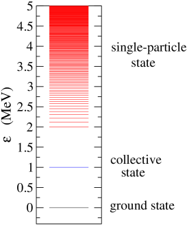
Figure 1: (Color online) The energy spectrum for the model calculation we employ. There is a collective vibrational state at 1 MeV, while single-particle states exist from 2 MeV with an exponentially increasing level density.

Figure 3 shows the penetrabilities thus obtained. The corresponding barrier distributions are shown in Fig. 3. The dotted and the dashed lines show the results without the channel couplings and those only with the collective excitation, respectively. The solid line shows the results with both the single-particle excitations and the collective excitation. We include the single-particle states up to $\epsilon_{\rm max}=$23 MeV with energy spacing of $\Delta\epsilon$=0.02 MeV. With this model space, the number of channels included is 1013 (we treat the low-lying single-particle states as discrete states when the energy spacing is larger than $\Delta\epsilon$). This result is obtained by generating the coupling matrix elements 30 times to take an ensemble average. We have found that the fluctuation around the average is small. For instance, at $E=100$ MeV, the averaged penetrability is $P=0.622$, whereas the root-mean-square deviation is 4.366$\times 10^{-3}$. As we mentioned in the previous section, the results shown in Fig. 2 are obtained with the constant coupling approximation. With a smaller value of $\epsilon_{\rm max}$, we have solved the coupled-channels equations exactly and have confirmed that the constant coupling approximation works qualitatively well.

The collective excitation leads to a double peaked structure of barrier distribution. One can see that the single-particle excitations suppress the penetrability at energies above the barrier, and at the same time smear the higher energy peak in the barrier distribution, although the main structure of the barrier distribution is still determined by the collective excitation. The single-particle excitations also lower the barrier and thus increase the penetrability at energies below the barrier, due to the well-known potential renormalization THAB94 .

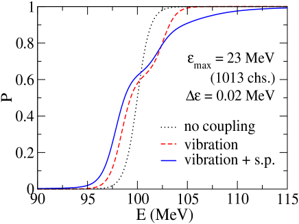
Figure 2: (Color online) The potential penetrability obtained with several methods. The dotted line is obtained without channel coupling, while the dashed line takes into account only the collective vibrational excitation. The solid line shows the result with both the collective and the single-particle excitations.

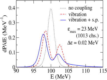
Figure 3: (Color online) The barrier distribution defined by the first derivative of the penetrability. The meaning of each line is the same as in Fig.3.

The $Q$-value distribution for the reflected flux is shown in Fig. 4 at four incident energies indicated in the figure. For a presentation purpose, we fold the discrete distribution with a Lorentz function,

$$g(\epsilon)=\frac{1}{\pi}\frac{\eta}{\epsilon^{2}+\eta^{2}},$$ (41)

with the width of $\eta=$0.2 MeV. That is, with the function defined by Eq. (13), we compute

$$F(E^{*}) =\int d\epsilon f(\epsilon)g(E^{*}-\epsilon)$$

$$=\sum_{n}|r_{n}|^{2}\frac{1}{\pi}\frac{\eta}{(E^{*}-\epsilon_{n})^{2}+\eta^{2}}.$$ (42)

In the figure, the peaks at $E^{*}=0\ {\rm MeV}$ and $E^{*}=1\ {\rm MeV}$ correspond to the elastic channel and the collective excitation channel, respectively. One can see that at energies well below the barrier the elastic and the collective peaks dominate in the distribution. As the energy increases, the single-particle excitations become more and more important. This behaviour is consistent with the experimental $Q$-value distribution observed for ¹⁶O+²⁰⁸Pb evers ; lin and ¹⁶O+¹⁸⁴W lin reactions. At energies above the barrier, the single-particle contribution is even larger than the contribution of the elastic and the collective peaks.

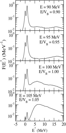
Figure 4: (Color online) The $Q$-value distribution for the reflected flux at four energies as indicated in the figure. It is obtained by smearing the discrete distribution with a Lorentzian function with the width of 0.2 MeV. The peaks at $E^{*}$=0 MeV and 1 MeV correspond to the elastic and the collective excitation channels, respectively.

III.2 Rotational coupling

Let us next consider the rotational coupling. For this purpose, we mock up the ²⁰Ne + ⁹²Zr system. That is, we consider the rotational excitations in ²⁰Ne up to the 4⁺ state and the single-particle excitations in ⁹²Zr. The energies of the rotational states are thus $\epsilon_{2^{+}}$ = 1.634 MeV and $\epsilon_{4^{+}}$ = 4.248 MeV for the 2⁺ and 4⁺ states, respectively. The values of the coupling strengths $F_{2}$ and $F_{4}$ in Eq. (24) are estimated with the collective model for the coupling form factor at the barrier position with the deformation parameters of $\beta_{2}$ = 0.46 and $\beta_{4}$ = 0.27. This yields $F_{2}=-6.892$ MeV and $F_{4}=-4.632$ MeV. For the single-particle excitations in ⁹²Zr, we consider the energy range of 2 MeV $\leq\epsilon\leq$ 16 MeV, with the exponential level density with $\rho_{0}=0.039$ MeV^-1 and $a=30/8$ MeV^-1. For the coupling strength, we use $w_{0}$ = 0.005 MeV and $\Delta=4.0$ MeV. These parameters are adjusted so that the rotational excitation in ²⁰Ne gives the main structure of the barrier distribution.

In the calculation shown below, we also include the mutual excitations of the projectile and the target nuclei. In order to avoid closed channels, we introduce the energy cutoff and include those channels whose total excitation energy is below 16 MeV. With this set-up, the number of channels included is 1688.

We use the Gaussian function for the potential for the relative motion with $V_{B}$ = 51.76 MeV and $s_{0}$ = 2.475 fm. This yields the same barrier height and the curvature as those with a Woods-Saxon potential with the parameters of $V_{0}$ = 59.9 MeV, $r_{0}$ = 1.2 fm, and $a$ = 0.63 fm for the ²⁰Ne + ⁹²Zr system. The reduced mass is taken to be 20$\times$ 92 $m_{N}$/112.

Figs. 6 and 6 show the penetrability and the barrier distribution for this model, respectively. The meaning of each line is the same as in Figs. 3 and 3 for the vibrational coupling. With only the collective rotational excitations, there are three eigenbarriers whose height is 48.2, 53.3, and 55.6 MeV. In contrast to the vibrational coupling, for the rotational coupling with a prolate deformation the main peak in the barrier distribution is not the lowest energy peak. For the parameters we use, the highest energy barrier carries a relatively small weight and the barrier distribution has only two visible peaks. The effect of single-particle excitations on the barrier distribution is similar to the case for the vibrational coupling and smears the higher energy peak in the barrier distribution.

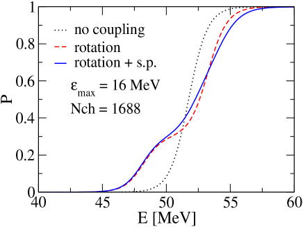
Figure 5: (Color online) The same as Fig. 3, but for the rotational coupling.

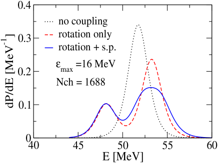
Figure 6: (Color online) The same as Fig. 3, but for the rotational coupling.

III.3 Quasi-elastic barrier distribution

Using the eigenbarriers and the corresponding weight factors obtained in the previous subsection, one can compute the quasi-elastic scattering cross sections and the quasi-elastic barrier distribution in a three-dimensional space. That is, in the eigen-channel representation, the quasi-elastic scattering cross section is given by qelbar ; ARN88 ,

$$\sigma_{\rm qel}(E,\theta)=\sum_{i}w_{i}\sigma_{\rm el}(E-\lambda_{i},\theta),$$ (43)

where $w_{i}=|U_{i0}|^{2}$ is the weight factor for the $i$-th eigen-channel and $\sigma_{\rm el}$ is the elastic scattering cross section. In order to calculate the elastic scattering cross sections, we use the Woods-Saxon potential indicated in the previous subsection. For the imaginary part of the optical potential, we assume an internal absorption, in which the imaginary part is well localized only inside the Coulomb barrier.

Fig. 7 shows the quasi-elastic barrier distribution obtained with the same $w_{i}$ and $\lambda_{i}$ as in the previous subsection for the one-dimensional model. We use the point difference formula with $\Delta E_{\rm c.m.}$= 2 MeV to calculate the quasi-elastic barrier distribution. The meaning of each line is the same as in Fig. 3. Because the quasi-elastic barrier distribution is by itself smeared more than the fusion barrier distribution qelbar , and also because we use the point difference formula rather than taking the derivative, the higher energy peak in the barrier distribution is more smeared by the single-particle excitations as compared to the one-dimensional calculation shown in the previous subsection. The difference between the dashed line (the collective excitations only) and the solid line (the collective + single-particle excitations) is similar to the difference in the experimental quasi-elastic barrier distribution between ²⁰Ne+⁹⁰Zr and ²⁰Ne+⁹²Zr systems. We therefore conclude that the single-particle excitations indeed provide a promising way to explain the difference in the quasi-elastic barrier distribution for the ²⁰Ne+^90,92Zr systems.

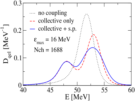
Figure 7: (Color online) The quasi-elastic barrier distribution for the ²⁰Ne+⁹²Zr system calculated with the weight factors and the eigenbarrier heights for the one-dimensional rotational model discussed in Sec. III B. The meaning of each line is the same as in Fig. 3.

IV Summary

We have studied the role of single-particle excitations in heavy-ion reactions at energies close to the Coulomb barrier. To this end, we employed a random matrix theory to describe the single-particle degrees of freedom. We applied the model to one dimensional barrier penetration problems by using the constant coupling approximation. In addition to the single-particle excitations, we also included the collective excitations with either a vibrational or a rotational character. We calculated the potential penetrability, the barrier distribution and the $Q$-value distribution. We also calculated the quasi-elastic barrier distribution for the ²⁰Ne + ⁹²Zr system using the eigenbarriers and their weight factors obtained with the one-dimensional model. Our calculations show that the single-particle excitations hinder the penetrability at energies above the barrier and smear the high energy part of the barrier distribution. In the $Q$-value distribution, we found that the contribution from the single-particle excitations increases significantly as the incident energy increases.

The experimental quasi-elastic barrier distributions are considerably different between ²⁰Ne + ^90,92Zr systems, despite that the coupled-channels calculations with collective excitations in the colliding nuclei lead to similar barrier distributions to each other. Our calculations imply that the difference can be indeed accounted for by the non-collective excitations in the target nuclei, as has been conjectured in Ref. piasecki

In order to make a quantitative comparison to the experimental data and draw a definite conclusion on the quasi-elastic barrier distribution for the ²⁰Ne + ^90,92Zr systems, it will be an interesting future work to extend our study presented in this paper to three-dimensional calculations without resorting to the constant coupling approximation. This is so espeically because the constant coupling approximation which we employed in this paper may introduce a significant phase error and thus leads to an inconsistent angular dependent interference between different partial waves. It may also be interesting to see whether this model accounts for the hindrance of fusion cross sections at deep sub-barrier energies recently found in several systems. For this purpose also, we would have to take into consideration the coordinate dependence of the coupling form factor, especially around the touching point of the colliding nucleiichikawa .

- (1) M. Dasgupta, D.J. Hinde, N. Rowley, and A.M. Stefanini, Annu. Rev. Nucl. Part. Sci. 48, 401(1998).
- (2) N. Rowley, G.R. Satchler and P.H. Stelson, Phys. Lett. B254 25, (1991).
- (3) L.R. Leigh, M. Dasgupta, D.J. Hinde, J.C. Mein, C.R. Morton, R.C. Lemmon, J.P. Lestone, J.O. Newton, H. Timmers, J.X. Wei, and N. Rowley, Phys. Rev. C52, 3151(1995).
- (4) H. Timmers, J.R. Leigh, M. Dasgupta, D.J. Hinde, R.C. Lemmon, J.C. Mein, C.R. Morton, J.O. Newton, and N. Rowley, Nucl. Phys. A584, 190 (1995).
- (5) K. Hagino and N. Rowley, Phys. Rev.C 69, 054610(2004).
- (6) Muhammad Zamrun F. and K. Hagino, Phys. Rev. C77, 014606 (2008).
- (7) K. Hagino, N. Rowley, A.T. Kruppa, Compt. Phys. Comm. 123, 143 (1999).
- (8) C.H. Dasso, S. Landowne, and A. Winther, Nucl. Phys.A405, 381(1983); A407, 221(1983).
- (9) K. Hagino, N. Takigawa, and A.B. Balantekin, Phys. Rev. C56, 2104 (1997).
- (10) M.A. Nagarajan, A.B. Balantekin, and N. Takigawa, Phys. Rev. C34, 894 (1986).
- (11) J.O. Newton, R.D. Butt, M. Dasgupta, D.J. Hinde, I.I. Gontchar, C.R. Morton, and K. Hagino, Phys. Rev. C70, 024605 (2004).
- (12) C.L. Jiang et al., Phys. Rev. Lett. 89, 052701 (2002); Phys. Rev. C79, 044601 (2009), and references therein.
- (13) M. Dasgupta et al., Phys. Rev. Lett. 99, 192701 (2007).
- (14) A.M. Stefanini et al., Phys. Rev. C78, 044607 (2008); Phys. Lett. B679, 95 (2009).
- (15) E. Piasecki, Ł. Świderski, W. Gawlikowicz, J. Jastrzebski, N. Keeley, M. Kisieliński, S. Kliczewski, A. Kordyasz, M. Kowalczyk, S. Khlebnikov, E. Koshchiy, E. Kozulin, T. Krogulski, T. Loktev, M. Mutterer, K. Piasecki, A. Piórkowska, K. Rusek, A. Staudt, M. Sillanpää, S. Smirnov, I. Strojek, G. Tiourin, W. H. Trzaska, A. Trzcińska, K. Hagino, and N. Rowley, Phys. Rev. C80, 054613 (2009).
- (16) Brookhaven National Laboratory, Evaluated Nuclear Structure Data File, http://www.nndc.bnl.gov/ensdf/. See references therein.
- (17) S. Raman, T.A. Walkiewicz, S. Kahane, E. Jurney, J. Sa, Z. Gacsi, J.W. Weil, K. Allaart, G. Bonsignori, and J.F. Shriner, Jr., Phys. Rev. C43, 521 (1991).
- (18) A.V. Ignatyuk, J.L. Weil, S. Raman, and S. Kahane, Phys. Rev. C47, 1504 (1993).
- (19) A. Diaz-Torres, D.J. Hinde, M. Dasgupta, G.J. Milburn, and J.A. Tostevin, Phys. Rev. C78, 064604 (2008).
- (20) D. Agassi, C.M. Ko, and H.A. Weidenmüller, Ann. Phys 107, 140(1977).
- (21) C.M. Ko, D. Agassi, and H.A. Weidenmüller, Ann. Phys 117, 237(1979).
- (22) D. Agassi, C.M. Ko, and H.A. Weidenmüller, Ann. Phys 117, 435 (1979).
- (23) D. Agassi, C.M. Ko, and H.A. Weidenmüller, Phys. Rev. C 18, 223(1978).
- (24) V.I. Zagrebaev, Ann. of Phys. (N.Y.) 197, 33 (1990).
- (25) T. Papenbrock and H.A. Weidenmüller, Rev. Mod. Phys. 79, 997 (2007).
- (26) H.A. Weidenmüller and G.E. Mitchell, Rev. Mod. Phys.,81, 539(2009).
- (27) G.E. Mitchell, A. Richter, and H.A. Weidenmüller, arXiv:1001.2422 [nucl-th].
- (28) C.W.J. Beenakker, Rev. Mod. Phys.,69, 731 (1997).
- (29) D.M. Brink, J. Neto, and H.A. Weidenmüller, Phys. Lett. 80B, 170 (1979).
- (30) N. Takigawa, K. Niita, Y. Okuhara, and S. Yoshida, Nucl. Phys. A371, 130 (1981).
- (31) K. Niita and N. Takigawa, Nucl. Phys. A397, 141 (1983).
- (32) M. Wilkinson, Phys. Rev. A41, 4645 (1990).
- (33) A. Bulgac, G.D. Dang, and D. Kusnezov, Phys. Rev. E54, 3468 (1997).
- (34) S. Mizutori and S. Aberg, Phys. Rev. E56, 6311 (1997).
- (35) C.M. Ko, H.J. Pirner, and H.A. Weidenmüller, Phys. Lett. B62, 248 (1976).
- (36) M.C. Nemes, Nucl.Phys A315, 457(1979).
- (37) R. Lipperheide, Nucl.Phys A260, 292(1976).
- (38) A.K. Kerman and S.E. Koonin, Phys. Scripta 10A, 118 (1974).
- (39) N. Takigawa, K. Hagino, M. Abe, and A.B. Balantekin, Phys. Rev. C49, 2630 (1994).
- (40) M. Evers, M. Dasgupta, D.J. Hinde, L.R. Gasques, M.L. Brown, R. Rafiei, and R.G. Thomas, Phys. Rev. C78, 034614 (2008).
- (41) C.J. Lin, H.M. Jia, H.Q. Zhang, F. Yang, X.X. Xu, F. Jia, Z.H. Liu, and K. Hagino, Phys. Rev. C79, 064603 (2009).
- (42) M.V. Andres, N. Rowley, and M.A. Nagarajan, Phys. Lett. B202, 292 (1988).
- (43) T. Ichikawa, K. Hagino, and A. Iwamoto, Phys. Rev. C75, 057603 (2007); Phys. Rev. C75, 064612 (2007); Phys. Rev. Lett. 103, 202701 (2009).