Shot noise and Coulomb effects on non-local electron transport in normal-superconducting-normal heterostructures

Abstract

We argue that Coulomb interaction can strongly influence non-local electron transport in normal-superconducting-normal structures and emphasize direct relation between Coulomb effects and non-local shot noise. In the tunneling limit non-local differential conductance is found to have an S-like shape and can turn negative at non-zero bias. At high transmissions crossed Andreev reflection yields positive noise cross-correlations and Coulomb anti-blockade of non-local electron transport.

I Introduction

Discreteness of electron charge has a number of fundamental physical consequences, such as, e.g., shot noise in mesoscopic conductors BB and Coulomb blockade of charge transfer in tunnel junctions SZ . About 10 years ago it was realized GZ01 ; LY1 that these two seemingly different phenomena are closely related to each other: Coulomb blockade turns out to be stronger in conductors with bigger shot noise. This fundamental relation was subsequently confirmed in experiments Pierre . A close link between shot noise and Coulomb blockade exists not only in normal conductors but also in hybrid normal-superconducting ($NS$) structures GZ09 , where doubling of elementary charge due to Andreev reflection becomes important.

Can the above relation be further extended to include non-local effects? A non-trivial example is provided by normal-superconducting-normal ($NSN$) systems where entanglement between electrons in different normal terminals can be realized. Non-local electron transport in such systems is determined by an interplay between elastic cotunneling (EC) and crossed Andreev reflection (CAR) and was recently investigated both experimentally Beckmann ; Teun ; Venkat ; Basel ; Beckmann2 and theoretically FFH ; KZ06 ; GKZ (see also further refs. therein). While non-interacting theory predicts that CAR never dominates over direct electron transfer (hence, no sign change of non-local signal could occur), both positive and negative non-local signals have been detected Beckmann ; Teun ; Basel ; Beckmann2 . It was argued that CAR could prevail over EC in the presence of Coulomb interactions LY or an external ac field GlZ09 . Negative non-local conductance was also predicted in interacting single-level quantum dots in-between normal and superconducting terminals Koenig .

Despite these developments no general theory describing the effect of electron-electron interactions on non-local transport in $NSN$ structures was available until now. Below we will construct such a theory and demonstrate that interaction effects in non-local transport and non-local shot noise in such systems are intimately related. This relation, however, turns out to be much more subtle than in the local case GZ01 ; LY1 ; GZ09 merely because of ($a$) a variety of different processes contributing to non-local shot noise and ($b$) positive cross-correlations which may occur in normal-superconducting hybrids BB ; AD (in contrast to normal conductors where cross-correlations of fluctuating currents are negative BB ). In tunnel $NSN$ systems EC and CAR provide respectively negative and positive contributions to non-local shot noise Pistolesi ; Chandrasekhar . Here we will analyze non-local shot noise beyond the tunneling limit and find that at higher transmissions also direct electron transfer can yield positive cross-correlations in addition to CAR. At full transmissions only positive cross-correlations due to CAR survive and yield Coulomb anti-blockade of non-local electron transport.

The paper is organized as follows. In Sec. 2 we describe our model and derive an effective action for $NSN$ system under consideration. In Sec. 3 we formulate the Langevin equations describing real time dynamics of fluctuating voltages and currents and derive the general expressions for both local and non-local current-current correlators describing shot noise in our system at arbitrary barrier transmissions and arbitrary frequencies. Sec. 4 is devoted to the effects of Coulomb interaction on both local and non-local conductances of our $NSN$ device. A brief summary of our key observations is presented in Sec. 5. Some technical details are outlined in Appendix.

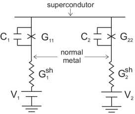
Figure 1: Schematics of the system under consideration.

II The model and effective action

We will consider a hybrid structure consisting of two normal electrodes coupled to a superconductor via $NS$ barriers with local subgap conductances $G_{11}$ and $G_{22}$ and capacitances $C_{1}$ and $C_{2}$ (Fig. 1). External voltages $V_{1}$ and $V_{2}$ are applied to normal electrodes via Ohmic shunts with conductances $G_{1}^{\rm sh}$ and $G_{2}^{\rm sh}$. Weak electromagnetic coupling between two $NS$ barriers (e.g. via modes propagating in the superconductor LY ) will be disregarded. The Hamiltonian of the system reads

$$H=H_{1}+H_{2}+H_{S}+H_{T,1}+H_{T,2},$$ (1)

where

$$H_{r}=\sum_{\alpha=\uparrow,\downarrow}\int d{\bm{x}}\hat{\psi}^{\dagger}_{r,\alpha}\left(-\frac{\nabla^{2}}{2m}-\mu\right)\hat{\psi}_{r,\alpha},\;\;r=1,2,$$

are the Hamiltonians of the normal metals, $m$ is electron mass, $\mu$ is the chemical potential,

$$H_{S}=\int d{\bm{x}}\bigg{[}\sum_{\alpha}\hat{\chi}^{\dagger}_{\alpha}\left(-\frac{\nabla^{2}}{2m}-\mu\right)\hat{\chi}_{\alpha}+\Delta\hat{\chi}^{\dagger}_{\uparrow}\hat{\chi}^{\dagger}_{\downarrow}+\Delta^{*}\hat{\chi}_{\downarrow}\hat{\chi}_{\uparrow}\bigg{]}$$

is the Hamiltonian of the superconductor with order parameter $\Delta$ and

$$H_{T,r}={\cal A}_{r}\sum_{\alpha,\beta=\uparrow,\downarrow}\big{[}t_{r}\,e^{i\varphi_{r}}\,\hat{\psi}^{\dagger}_{\beta}\hat{\chi}_{r,\alpha}+t_{r}^{*}\,e^{-i\varphi_{r}}\,\hat{\chi}_{r,\alpha}^{\dagger}\hat{\psi}_{\beta}\big{]}$$ (2)

are tunneling Hamiltonians describing transfer of electrons across the contacts with area ${\cal A}_{r}$ and tunneling amplitude $t_{r}$. For the sake of simplicity we will assume that both $NS$ barriers are uniform implying that all $N_{r}=k_{F}^{2}{\cal A}_{r}/4\pi$ conducting channels in the $r$-th barrier are characterized by equal transmission values

$$T_{r}={4\pi^{2}\nu_{r}\nu_{S}|t_{r}|^{2}}/{\left(1+\pi^{2}\nu_{r}\nu_{S}|t_{r}|^{2}\right)^{2}}.$$ (3)

where $\nu_{j}$ ($j=1,2,S$) is the density of states in the corresponding terminal. Accordingly, in the low energy limit to be considered below local subgap conductances are defined as BTK $G_{rr}=(2e^{2}/\pi)N_{r}\tau_{r}$, where $\tau_{r}=T_{r}^{2}/(2-T_{r})^{2}$ are effective Andreev transmissions of $NS$ barriers. Finally, we note that fluctuating phases $\varphi_{r}$ introduced in Eq. (2) are linked to the voltage drops across the barriers $v_{r}$ by means of the standard relation $\dot{\varphi}_{r}=ev_{r}$ and are treated as quantum operators.

As usually, we eliminate fermionic variables and express the kernel $J$ of the Keldysh evolution operator via path integral over the phase fields SZ

$$J=\int\prod_{r=1,2}{\cal D}\varphi^{F}_{r}{\cal D}\varphi_{r}^{B}\exp(iS_{\rm env}[\varphi]+iS_{T}[\varphi]),$$ (4)

where $\varphi^{F}_{r}$ and $\varphi_{r}^{B}$ are fluctuating phases defined respectively on the forward and backward branches of the Keldysh contour, $S_{\rm env}$ is the action of electromagnetic environment and the term $iS_{T}$ accounts for electron transfer between the terminals. In the case of linear Ohmic environment considered here one has SZ

$$iS_{\rm env} = \sum_{r=1,2}\bigg{[}i\int dt\frac{(eV_{r}-\dot{\varphi}_{r})(-C_{r}\dot{\varphi}_{r}^{-}+G_{r}^{\rm sh}\varphi^{-}_{r})}{e^{2}}$$ (5)

$$-\,\frac{G_{r}^{\rm sh}}{2e^{2}}\int dtdt^{\prime}\varphi^{-}_{r}(t)M(t-t^{\prime})\varphi^{-}_{r}(t^{\prime})\bigg{]},$$

where $\varphi_{r}=(\varphi_{r}^{F}+\varphi_{r}^{B})/2$, $\varphi^{-}_{r}=\varphi_{r}^{F}-\varphi^{B}_{r}$ and

$$M(t)=\int\frac{d\omega}{2\pi}e^{i\omega t}\omega\coth\frac{\omega}{2T}=-\frac{\pi T^{2}}{\sinh^{2}(\pi Tt)}.$$

The term $iS_{T}$ reads

$$iS_{T}={\rm tr}\ln{\cal G}^{-1},\quad{\cal G}^{-1}=\left(\begin{array}[]{ccc}\check{G}_{1}^{-1}&\check{t}_{1}&0\\ \check{t}_{1}^{\dagger}&\check{G}_{S}^{-1}&\check{t}_{2}\\ 0&\check{t}_{2}^{\dagger}&\check{G}_{2}^{-1}\end{array}\right),$$ (9)

where $4\times 4$ matrices $\check{G}_{j}^{-1}$ represent the inverse Keldysh Green functions of (isolated) normal ($j=1,2$) and superconducting ($j=S$) terminals and $\check{t}_{r}$ is diagonal $4\times 4$ matrix in the Nambu - Keldysh space

$$\check{t}_{r}=\left(\begin{array}[]{cccc}-t_{r}e^{-i\varphi_{r}^{F}}&0&0&0\\ 0&t_{r}e^{-i\varphi_{r}^{B}}&0&0\\ 0&0&t_{r}e^{i\varphi_{r}^{F}}&0\\ 0&0&0&-t_{r}e^{i\varphi_{r}^{B}}\end{array}\right).$$ (14)

After some exact manipulations we obtain

$$iS_{T}=\,{\rm tr}\,\ln\big{[}\check{1}-\check{t}_{1}^{\dagger}\check{G}_{1}\check{t}_{1}\check{G}_{S}-\check{t}_{2}^{\dagger}\check{G}_{2}\check{t}_{2}\check{G}_{S}\big{]}.$$ (15)

While the expression (15) for the action remains formally exact it is still too complicated to be directly employed in our calculations. In order to proceed we will make several additional steps which yield necessary simplifications.

As a first step, we restrict ourselves to the limit of high conductances

$$g_{r}=2\pi(G_{r}^{\rm sh}+G_{rr})/e^{2}\gg 1,$$ (16)

in which case phase fluctuations are weak and it suffices to expand the action (15) to the second order in $\varphi^{-}_{r}$, cf., e.g., GZ01 ; GZ09 ; Schmid . Technically, we first expand the matrices $\check{t}_{r}$ to the second order in the quantum phases $\varphi^{-}_{r}$, i.e. we make a replacement

$$\check{t}_{r}\to\check{t}_{r}(\varphi_{r})\left(\check{1}-i\frac{\varphi^{-}_{r}}{2}\check{\Lambda}-\frac{\varphi_{r}^{-2}}{4}\check{1}\right).$$ (17)

Here $\check{t}_{r}(\varphi_{r})$ is defined by Eq. (14) with $\varphi^{F,B}_{r}$ being replaced by the classical phase $\varphi_{r}$, and $\check{\Lambda}$ is a diagonal matrix with non-zero elements $\Lambda_{11}=1$, $\Lambda_{22}=-1$, $\Lambda_{33}=-1$ and $\Lambda_{44}=1$. Accordingly, we can write the product $\check{t}_{r}^{\dagger}\check{G}_{r}\check{t}_{r}$ in the form

$$\check{t}_{r}^{\dagger}\check{G}_{r}\check{t}_{r}=\check{\Sigma}_{r}+\check{\Sigma}_{r}^{(1)}+\check{\Sigma}_{r}^{(2)}+{\cal O}(\varphi^{-3}_{r}),$$ (18)

where we defined the self-energies

$$\check{\Sigma}_{r} = \check{t}_{r}^{\dagger}(\varphi_{r})\check{G}_{r}\check{t}_{r}(\varphi_{r}),$$ (19)

$$\check{\Sigma}_{r}^{(1)} = \frac{i}{2}\big{[}\varphi^{-}_{r}\check{\Lambda},\check{\Sigma}_{r}\big{]},$$

$$\check{\Sigma}_{r}^{(2)} = -\frac{1}{4}\big{\{}\varphi^{-2}_{r}\check{1},\check{\Sigma}_{r}\big{\}}+\frac{1}{4}\varphi^{-}_{r}\check{\Lambda}\check{\Sigma}_{r}\varphi^{-}_{r}\check{\Lambda}.$$

In order to evaluate $\check{\Sigma}_{r}$ we employ the Keldysh Green functions of the normal leads

$$\check{G}_{r}=(\hat{G}_{r}^{R}+\hat{G}^{A}_{r})\otimes\hat{\sigma}_{z}/2+(\hat{G}_{r}^{R}-\hat{G}^{A}_{r})\otimes\hat{Q}_{r}\hat{\sigma}_{z}/2.$$ (20)

Here the $2\times 2$ matrices $\hat{G}_{r}^{R,A}$ and $\hat{Q}_{r}$ are defined as

$$\hat{G}_{r}^{R,A}=\left(\begin{array}[]{cc}G^{R,A}_{r}&0\\ 0&G^{R,A+}_{r}\end{array}\right),\;\hat{Q}_{r}=\left(\begin{array}[]{cc}1-2n_{r}&2n_{r}\\ 2-2n_{r}&2n_{r}-1\end{array}\right),$$ (25)

where $n_{r}$ is the quasiparticle distribution function in the $r$-th normal lead. In equilibrium it coincides with the Fermi function $n_{r}=1/(1+\exp(E/T))$. Neglecting the proximity effect in the normal leads and performing the summation over the corresponding electron states, we express the zeroth order self-energies (19) in the form

$$\check{\Sigma}_{r}(\varphi_{r},\bm{r})=\frac{\Gamma_{r}}{2i}h_{r}(\bm{r})\left(\begin{array}[]{c}\hat{\sigma}_{z}e^{i\varphi_{r}}\hat{Q}_{r}e^{-i\varphi_{r}}\;\;\;\;\;\;0\\ 0\;\;\;\;\;\;\hat{\sigma}_{z}e^{-i\varphi_{r}}\hat{Q}_{r}e^{i\varphi_{r}}\end{array}\right),$$ (28)

with $\Gamma_{r}=2\pi\nu_{r}|t_{r}|^{2}$. The function $h_{r}(\bm{r})$ in this expression differs from zero only at the interface of the $r$-th junction and it obeys the following normalization condition

$$\int d^{3}\bm{r}\,h_{r}(\bm{r})=N_{r}.$$ (29)

For the sake of simplicity, in what follows we will assume that the barrier cross-sections remain sufficiently small and put $h_{r}(\bm{r})=N_{r}\delta(\bm{r}-\bm{r}_{r})$. This assumption just implies that each of the barriers has $N_{r}$ conducting channels with identical transmissions $T_{r}$ (3, as we already indicated above. In this case we can reduce the full coordinate dependence of the Green functions to that on the two indices $i$ and $j$ which label the barriers and, hence, can take only two values 1 and 2. Accordingly, e.g., the Green function $\check{G}_{S}(\bm{r},\bm{r}^{\prime})$ reduces to the $2\times 2$ matrix in the ”junction space” $\check{G}_{S}^{ij}$. In addition we should bear in mind that $\check{G}_{S}^{ij}$ are the matrices in the space of conducting channels.

We note that the above assumptions are not really restrictive since they do not affect the general structure of our effective action to be derived below. At the same time they allow to establish relatively simple expressions for the parameters entering in the action. Expanding the action (15) in powers of $\varphi^{-}_{r}$ we arrive at the following expression

$$iS_{T} = -\,{\rm tr}\,\left[\check{K}\left(\check{\Sigma}_{1}^{(1)}+\check{\Sigma}_{2}^{(1)}\right)\check{G}_{S}\right]$$ (30)

$$-\,{\rm tr}\,\left[\check{K}\left(\check{\Sigma}_{1}^{(2)}+\check{\Sigma}_{2}^{(2)}\right)\check{G}_{S}\right]$$

$$-\,\frac{1}{2}\,{\rm tr}\,\left[\left(\check{K}\left(\check{\Sigma}_{1}^{(1)}+\check{\Sigma}_{2}^{(1)}\right)\check{G}_{S}\right)^{2}\right],$$

where we define the operator

$$\check{K}=\big{[}1-\check{\Sigma}_{1}\check{G}_{S}-\check{\Sigma}_{2}\check{G}_{S}\big{]}^{-1}.$$ (31)

Our second step allows to establish an explicit expression for the operator (31). Namely, in the interesting for us low energy limit

$$T,eV_{r}\ll|\Delta|$$ (32)

we can set the energy argument $E$ in the superconductor Green function $\check{G}_{S}(E)$ equal to zero. After that $\check{G}_{S}$ reduces to the time/energy independent matrix

$$\check{G}_{S}(E=0)=\big{(}G_{S}^{R}+G_{S}^{A}\big{)}\otimes({\hat{\sigma}_{z}}/{2}),$$ (33)

where we introduced the retarded and advanced Green functions of the superconductor $G^{R}_{S}$ and $G^{A}_{S}$. In the limit $E\to 0$ they are equal to each other both being $4\times 4$ matrices in the Nambu $\otimes$ ”junction” space

$$G_{S}^{R}=G_{S}^{A}=\left(\begin{array}[]{cccc}G^{R}_{11}&F^{R}_{11}&G^{R}_{12}&F^{R}_{12}\\ F^{R}_{11}&-G^{R}_{11}&F_{12}&-G_{12}^{R}\\ G^{R}_{21}&F^{R}_{21}&G_{22}^{R}&F_{22}^{R}\\ F^{R}_{21}&-G^{R}_{21}&F_{22}^{R}&-G_{22}^{R}\\ \end{array}\right).$$ (38)

In addition, each of the matrix elements in Eq. (38) is itself a matrix in the channel space. For instance, $G^{R}_{11}$ and $G^{R}_{12}$ are respectively $N_{1}\times N_{1}$ and $N_{1}\times N_{2}$ matrices, while matrices $G^{R}_{21}$ and $G^{R}_{22}$ have dimensions $N_{2}\times N_{1}$ and $N_{2}\times N_{2}$ respectively.

As the Keldysh Green function (33) depends neither on time nor on the quasiparticle distribution function, it commutes with the phase factors $e^{\pm i\varphi_{r}(t)}$ entering the self-energies. This observation combined with the multiplication rule for the $Q-$matrices, $\hat{Q}_{1}\hat{Q}_{2}=\hat{1}-\hat{Q}_{1}+\hat{Q}_{2}$, allows us to express the operator $\check{K}$ (31) as a linear combination of these matrices:

$$\check{K}(t,t^{\prime})=[(K_{R}+K_{A})/2]\otimes\hat{1}\,\delta(t-t^{\prime})$$ (39)

$$-\,i(\Gamma_{1}/2)K_{R}X_{1}K_{A}\otimes\,e^{i\varphi_{1}(t)}\hat{\sigma}_{z}\hat{Q}_{1}(t-t^{\prime})\hat{\sigma}_{z}e^{-i\varphi_{1}(t^{\prime})}$$

$$-\,i(\Gamma_{1}/2)K_{R}X_{2}K_{A}\otimes\,e^{-i\varphi_{1}(t)}\hat{\sigma}_{z}\hat{Q}_{1}(t-t^{\prime})\hat{\sigma}_{z}e^{i\varphi_{1}(t^{\prime})}$$

$$-\,i(\Gamma_{2}/2)K_{R}X_{3}K_{A}\otimes\,e^{i\varphi_{2}(t)}\hat{\sigma}_{z}\hat{Q}_{2}(t-t^{\prime})\hat{\sigma}_{z}e^{-i\varphi_{2}(t^{\prime})}$$

$$-\,i(\Gamma_{2}/2)K_{R}X_{4}K_{A}\otimes\,e^{-i\varphi_{2}(t)}\hat{\sigma}_{z}\hat{Q}_{2}(t-t^{\prime})\hat{\sigma}_{z}e^{-i\varphi_{2}(t^{\prime})}.$$

Here $4\times 4$ matrices $X_{j}$ are defined as follows

$$X_{1}=\left(\begin{array}[]{cccc}G^{R}_{11}&F^{R}_{11}&G^{R}_{12}&F^{R}_{12}\\ 0&0&0&0\\ 0&0&0&0\\ 0&0&0&0\\ \end{array}\right),$$ (44)

$$X_{2}=\left(\begin{array}[]{cccc}0&0&0&0\\ F^{R}_{11}&-G^{R}_{11}&F^{R}_{12}&-G^{R}_{12}\\ 0&0&0&0\\ 0&0&0&0\\ \end{array}\right),$$ (49)

$$X_{3}=\left(\begin{array}[]{cccc}0&0&0&0\\ 0&0&0&0\\ G^{R}_{21}&F^{R}_{21}&G^{R}_{22}&F^{R}_{22}\\ 0&0&0&0\\ \end{array}\right),$$ (54)

$$X_{4}=\left(\begin{array}[]{cccc}0&0&0&0\\ 0&0&0&0\\ 0&0&0&0\\ F^{R}_{21}&-G^{R}_{21}&F^{R}_{22}&-G^{R}_{22}\\ \end{array}\right),$$ (59)

while $4\times 4$ matrices $K_{R,A}$ read

$$K_{R}=K_{A}^{*}=\left[1+i\frac{\Gamma_{1}}{2}(X_{1}+X_{2})+i\frac{\Gamma_{2}}{2}(X_{3}+X_{4})\right]^{-1}.$$ (60)

Having established the expression for the operator $\check{K}$ we can now substitute it into the action (30). Proceeding along these lines and going trough a straightforward but rather tedious calculation we arrive at the result which still turns out to be too complicated for our present purposes. Further simplification amounts to neglecting local interference terms involving the products of the Green functions $G_{11}^{R}$, $F_{11}^{R}$, $G_{22}^{R}$ and $F_{22}^{R}$. Technically this step is equivalent to replacing these Green functions by their averaged-over-disorder values, which read

$$\langle G_{11}^{R}\rangle=\langle G_{22}^{R}\rangle=0,\;\;\;\langle F_{11}^{R}\rangle=\langle F_{22}^{R}\rangle=-\pi\nu_{S}.$$ (61)

After this step we immediately arrive at the central result of this section

$$iS_{T} = iS_{11}+iS_{22}+iS_{12},$$ (62)

where

$$iS_{11}=-i\frac{G_{11}}{e^{2}}\int dt\dot{\varphi}_{1}\varphi_{1}^{-}-\int dtdt^{\prime}\frac{\varphi^{-}_{1}(t)\,\tilde{\cal S}_{11}^{tt^{\prime}}\,\varphi^{-}_{1}(t^{\prime})}{2e^{2}},$$ (63)

$$iS_{12} = i\frac{G_{12}}{e^{2}}\int dt\,\big{(}\dot{\varphi}_{1}\varphi_{2}^{-}+\dot{\varphi}_{2}\varphi_{1}^{-}\big{)}$$ (64)

$$-\,\int dtdt^{\prime}\frac{\varphi^{-}_{1}(t)\,\tilde{\cal S}_{12}^{tt^{\prime}}\,\varphi^{-}_{2}(t^{\prime})}{e^{2}}$$

and the term $iS_{22}$ is obtained by interchanging the indices $1\leftrightarrow 2$ in Eq. (63). The functions $\tilde{\cal S}_{rl}^{tt^{\prime}}$ read

$$\tilde{\cal S}_{11}^{tt^{\prime}} = G_{11}M(t-t^{\prime})\big{(}1-\beta_{1}+\beta_{1}\cos[2\varphi_{1}^{tt^{\prime}}]\big{)}$$ (65)

$$+\,2G_{12}M(t-t^{\prime})\big{(}\alpha_{1}-\eta_{1}\cos[2\varphi_{1}^{tt^{\prime}}]\big{)}$$

$$+(G_{12}/2)M(t-t^{\prime})\big{(}\kappa_{1}^{+}\cos[\varphi_{1}^{tt^{\prime}}+\varphi_{2}^{tt^{\prime}}]$$

$$+\,\kappa_{1}^{-}\cos[\varphi_{1}^{tt^{\prime}}-\varphi_{2}^{tt^{\prime}}]\big{)},$$

$$\tilde{\cal S}_{12}^{tt^{\prime}} = -G_{12}M(t-t^{\prime})\big{(}1-\beta_{1}+\beta_{1}\cos[2\varphi_{1}^{tt^{\prime}}]\big{)}$$ (66)

$$-G_{12}M(t-t^{\prime})\big{(}1-\beta_{2}+\beta_{2}\cos[2\varphi_{2}^{tt^{\prime}}]\big{)}$$

$$+\,(G_{12}/2)M(t-t^{\prime})\big{(}\gamma_{+}\cos[\varphi_{1}^{tt^{\prime}}+\varphi_{2}^{tt^{\prime}}]$$

$$-\,\gamma_{-}\cos[\varphi_{1}^{tt^{\prime}}-\varphi_{2}^{tt^{\prime}}]\big{)}.$$

Here we denoted $\varphi_{r}^{tt^{\prime}}=\varphi_{r}(t)-\varphi_{r}(t^{\prime})$ and introduced Andreev Fano factors $\beta_{r}=1-\tau_{r}$.

The zero bias non-local subgap conductance $G_{12}$ as well as the parameters $\alpha_{r},\eta_{r},\kappa_{r},\gamma$ are expressed as traces of certain combinations of the matrices $K_{R}$, $K_{A}$ and $X_{j}$, as described in Appendix. In order to reduce them to a tractable form we further assume that normal state resistance $R_{\xi}$ of the superconducting wire segment of length equal to the superconducting coherence length $\xi$ remains much smaller than normal resistances of the barriers GKZ , i.e.

$$e^{2}N_{r}T_{r}R_{\xi}/\pi\ll 1.$$ (67)

This condition is usually well satisfied for generic systems. Eq. (67) enables one to treat the Green functions connecting the two junctions as small parameters and expand the traces in Eqs. (86)-(88) in powers of $G_{12}^{R},G_{21}^{R},F_{12}^{R}$ and $F_{21}^{R}$. Keeping the leading corrections $\propto G_{12}^{R}G_{21}^{R}$ and $\propto F_{12}^{R}F_{21}^{R}$ and making use of the fact that $G_{12}^{R}G_{21}^{R}$ becomes equal to $F_{12}^{R}F_{21}^{R}$ after averaging over disorder, we arrive at explicit expressions for the parameters

$$\alpha_{r} = \tau_{r}(1-2\tau_{r})/\sqrt{\tau_{1}\tau_{2}},$$

$$\eta_{r} = 2\tau_{r}(1-\tau_{r})/\sqrt{\tau_{1}\tau_{2}},$$

$$\kappa_{r}^{\pm} = \pm(4\tau_{r}-3)+1/{\sqrt{\tau_{1}\tau_{2}}}\;\;(r=1,2),$$

$$\gamma_{\pm} = \pm 1+\big{(}{1-2\tau_{1}-2\tau_{2}+4\tau_{1}\tau_{2}}\big{)}/{\sqrt{\tau_{1}\tau_{2}}},$$ (68)

and for zero bias non-local conductance

$$G_{12}=\frac{2e^{2}N_{1}N_{2}\tau_{1}\tau_{2}}{\pi^{3}\nu_{S}^{2}}G^{R}_{12}G^{R}_{21}.$$ (69)

In the case of diffusive superconductors one has to further average Eq. (69) over disorder. In a simple quasi-one-dimensional geometry this averaging yields GKZ $G_{12}=G_{11}G_{22}R_{\xi}\,e^{-d/\xi}/2$, where $d$ is the distance between two $NS$ barriers.

It is important to emphasize that all order terms in $t_{r}$ are fully accounted for in Eqs. (63)-(68), i.e. our action applies for arbitrary transmission values $T_{1,2}$ (or $\tau_{1,2}$) ranging from zero to one and – similarly to $NS$ systems GZ09 – entering in the combination $T_{r}^{2}/(2-T_{r})^{2}$ representing Andreev transmissions $\tau_{r}$.

III Langevin equations and shot noise

The quadratic in $\varphi^{-}_{1,2}$ action is equivalent to the Langevin equations Schmid ; AES ; GZ92

$$C_{1}\dot{v}_{1}+(G_{1}^{\rm sh}+G_{11})v_{1}-G_{12}v_{2}=G_{1}^{\rm sh}V_{1}+\xi^{\rm sh}_{1}+\xi_{1},$$

$$C_{2}\dot{v}_{2}+(G_{2}^{\rm sh}+G_{22})v_{2}-G_{12}v_{1}=G_{2}^{\rm sh}V_{2}+\xi^{\rm sh}_{2}+\xi_{2},$$ (70)

which describe the current balance in our system. Here $\xi_{r}^{\rm sh}$ are stochastic variables with pair correlators

$$\langle\xi_{r}^{\rm sh}(t)\xi_{r}^{\rm sh}(t^{\prime})\rangle=G_{r}^{\rm sh}M(t-t^{\prime})$$ (71)

describing Gaussian current noise in the shunt resistors, while the variables $\xi_{r}$ with the correlators

$$\langle\xi_{r}(t)\xi_{l}(t^{\prime})\rangle=\tilde{\cal S}_{rl}^{tt^{\prime}}$$ (72)

describe shot noise in $NS$ barriers. Note that we ignore the electro-magnetic coupling between the two junctions, i.e. mutual capacitance between the normal wires, propagating modes in the superconducting wire LY and similar effects.

Let us first ”turn off” electron-electron interactions by taking the limit $1/G_{1,2}^{\rm sh}\to 0$ and, hence, setting $\varphi_{r}=eV_{r}t$. Defining the non-local noise spectrum as ${\cal S}_{rl}(\omega)=2\int dt\,\tilde{\cal S}_{rl}^{tt^{\prime}}\exp(-i\omega(t-t^{\prime}))$, from Eq. (66) we obtain

$${\cal S}_{12}(\omega)=-2G_{12}(2-\beta_{1}-\beta_{2})W(\omega,0)$$ (73)

$$-\,2G_{12}\beta_{1}W(\omega,2V_{1})-2G_{12}\beta_{2}W(\omega,2V_{2})$$

$$+\,G_{12}\gamma_{+}W(\omega,V_{1}+V_{2})-G_{12}\gamma_{-}W(\omega,V_{1}-V_{2}),$$

where

$$W(\omega,V)=\frac{1}{2}\sum_{\pm}(\omega\pm eV)\coth\frac{\omega\pm eV}{2T}.$$ (74)

This is the first key result of the present paper. Eqs. (73), (74) fully determine non-local shot noise correlations in $NSN$ structures at subgap energies $T,\omega,eV_{r}\ll|\Delta|$. In the tunneling limit $T_{1,2}\ll 1$ we have $\gamma_{\pm}=4/T_{1}T_{2}\gg\beta_{1,2}\simeq 1$ and Eq. (73) is dominated by the last two terms which further reduce to the result Pistolesi in the limit $\omega\to 0$. One of these contributions $\propto\gamma_{-}$ is due to EC and describes negative shot noise correlations while the other one $\propto\gamma_{+}$ comes from CAR and accounts for positive cross-correlations of fluctuating currents. Provided one of the voltages, say $V_{1}$, equals to zero, these EC and CAR terms exactly cancel each other for any $V_{2}$, i.e. ${\cal S}_{12}(0)$ tends to zero in the tunneling limit.

At higher transmissions $\tau_{1,2}$ the value $\gamma_{-}$ becomes negative thus implying positive cross-correlations produced by direct electron transfer at such values of $\tau_{1,2}$ in addition to CAR. In the limit of fully transparent barriers $\tau_{1,2}=1$ one has $\beta_{1,2}=\gamma_{-}=0$. Then Eq. (73) yields

$${\cal S}_{12}(0)=-8TG_{12}+2eG_{12}(V_{1}+V_{2})\coth\frac{e(V_{1}+V_{2})}{2T}.$$ (75)

At $T\to 0$ only positive cross-correlations due to CAR survive whereas no direct electron transfer contribution to shot noise occurs for fully open barriers. Accordingly, no non-local shot noise is expected in this case at $V_{1}=-V_{2}$ and $T\to 0$. We also note that noise correlations in clean $NSN$ systems and in the specific limit $T_{1}=T_{2}$, $V_{1}=V_{2}$, $T=\omega=0$ have been recently studied in Ref. Melin, . The result of this paper is consistent with our Eq. (73) in the corresponding limit.

For completeness we also provide the expression for the local noise $S_{11}(\omega)$, which is given by the Fourier transform of Eq. (65) and reads

$$S_{11}(\omega)=2G_{11}\left[(1-\beta_{1})W(\omega,0)+\beta_{1}W(\omega,2V_{1})\right]$$

$$+\,4G_{12}\left[\alpha_{1}W(\omega,0)-\eta_{1}W(\omega,2V_{1})\right]$$

$$+\,G_{12}\kappa_{1}^{+}W(\omega,V_{1}+V_{2})+G_{12}\kappa_{1}^{-}W(\omega,V_{1}-V_{2}).$$ (76)

IV Interaction correction to the current

Now we again “turn on” electron-electron interactions and evaluate the current $I_{1}$ across the first barrier. Solving Eqs. (70) perturbatively in $1/g_{r}\ll 1$, in the lowest non-trivial order in this parameter we get

$$I_{1}=G_{11}V_{1}-G_{12}V_{2}-\langle\xi_{1}\rangle.$$ (77)

Here the average $\langle\xi_{1}\rangle$ does not vanish since according to Eqs. (65), (66) the noise $\xi_{1}$ depends on the phases $\varphi_{1,2}$, which, in turn depend on $\xi_{1,2}$ by virtue of Eqs. (70). Hence, we obtain

$$\langle\xi_{1}\rangle=\left\langle\delta\varphi_{1}\;{\partial\xi_{1}}/{\partial\varphi_{1}}\right\rangle+\left\langle\delta\varphi_{2}\;{\partial\xi_{1}}/{\partial\varphi_{2}}\right\rangle,$$ (78)

where the phase fluctuations $\delta\varphi_{r}$ are found from Eqs. (70) and read

$$\delta\varphi_{r}(t)=e\int_{-\infty}^{t}dt^{\prime}\frac{1-e^{-(t-t^{\prime})/\tau_{RC}}}{G_{r}^{\rm sh}}\xi_{r}(t^{\prime}).$$ (79)

Here we have assumed $G_{12}\ll G_{rr}\ll G_{r}^{\rm sh}$ and introduced the $RC-$time $\tau_{RC}=C_{r}/G_{r}^{\rm sh}$. Substituting this expression into Eq. (78) we find

$$\frac{\langle\xi_{1}\rangle}{e}=\sum_{r=1,2}\int_{-\infty}^{t}dt^{\prime}\frac{1-e^{-\frac{t-t^{\prime}}{\tau_{RC}}}}{G_{r}^{\rm sh}}\left.\frac{\partial\langle\xi_{1}(t)\xi_{r}(t^{\prime})\rangle}{\partial\varphi_{r}(t)}\right|_{\varphi_{r}=eV_{r}t}.$$ (80)

Making use of Eqs. (65), (66) and performing the time integral in Eq. (80) we get the current through the first junction in the form

$$I_{1}=G_{11}V_{1}-G_{12}V_{2}$$

$$-\,\frac{2G_{11}\beta_{1}-4G_{12}\eta_{1}}{g_{1}}F_{0}(2V_{1})+\frac{2G_{12}\beta_{2}}{g_{2}}F_{0}(2V_{2})$$

$$-\delta G_{+}F_{0}(V_{1}+V_{2})-\delta G_{-}F_{0}(V_{1}-V_{2}),$$ (81)

where $\delta G_{\pm}=G_{12}\left({\kappa^{\pm}_{1}}/{g_{1}}+{\gamma_{\pm}}/{g_{2}}\right)$ and

$$F_{0}(V)=\,{\rm Re}\,\left[-V\Psi\left(1+i\frac{eV}{2\pi T}\right)\right.$$

$$\left.+\,\left(V-\frac{i}{e\tau_{RC}}\right)\Psi\left(1+\frac{1}{2\pi T\tau_{RC}}+i\frac{eV}{2\pi T}\right)\right].$$ (82)

Accordingly the local and non-local differential conductances read

$$\frac{\partial I_{1}}{\partial V_{1}}=G_{11}-\frac{4G_{11}\beta_{1}-8G_{12}\eta_{1}}{g_{1}}F(2V_{1})$$

$$-\,\delta G_{+}F(V_{1}+V_{2})-\delta G_{-}F(V_{1}-V_{2}),$$ (83)

and

$$\frac{\partial I_{1}}{\partial V_{2}}=-G_{12}\left[1-\frac{4\beta_{2}}{g_{2}}F(2V_{2})\right]$$

$$-\,\delta G_{+}F(V_{1}+V_{2})+\delta G_{-}F(V_{1}-V_{2}),$$ (84)

where

$$F(V)=\,{\rm Re}\,\left[\Psi\left(1+\frac{1}{2\pi T\tau_{RC}}+i\frac{eV}{2\pi T}\right)\right.$$

$$+\,\left(\frac{1}{2\pi T\tau_{RC}}+i\frac{eV}{2\pi T}\right)\Psi^{\prime}\left(1+\frac{1}{2\pi T\tau_{RC}}+i\frac{eV}{2\pi T}\right)$$

$$\left.-\,\Psi\left(1+i\frac{eV}{2\pi T}\right)-i\frac{eV}{2\pi T}\Psi^{\prime}\left(1+i\frac{eV}{2\pi T}\right)\right],$$ (85)

and $\Psi(x)$ is the digamma function. Eqs. (83), (84) together with Eq. (85) define the conductance matrix of our $NSN$ device and represent the second key result of our paper.

In the interaction correction to the local conductance in (83) we recover the Coulomb blockade term GZ09 $\propto\beta_{1}$ and, in addition, three non-local contributions. The first of them $\propto\eta_{1}$ enhances the conductance, while the second one $\propto\delta G_{+}$ provides additional Coulomb suppression of $\partial I_{1}/\partial V_{1}$. The last term $\propto\delta G_{-}$ can be both positive (at $\tau_{1,2}\ll 1$) and negative (at bigger $\tau_{1,2}$) implying the tendency to Coulomb anti-blockade in the latter case. The first term $\propto\beta_{2}$ in Eq. (84) has an opposite sign as compared to $G_{12}$ (thus implying Coulomb blockade), while the second one $\propto\delta G_{+}$ yields Coulomb anti-blockade. Finally, the third $\propto\delta G_{-}$ tends to suppress or enhance the absolute value of the non-local conductance respectively for $\delta G_{-}>0$ and $\delta G_{-}<0$.

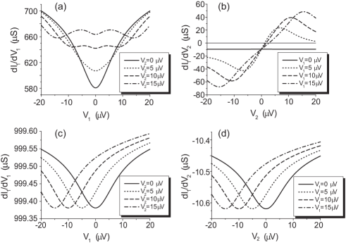
Figure 2: Local (a,c) and non-local (b,d) differential conductances defined respectively in Eqs. (83) and (84). The parameters of the system are: $T=20$ mK, $G_{11}=1$ mS, $G_{12}=10$ $\mu$S, $g_{1}=g_{2}=516$. The dependencies (a) and (b) are plotted at small transmissions $T_{1}=0.063$, $T_{2}=0.11$, while the graphs (c) and (d) correspond to fully open barriers $T_{1}=T_{2}=1$.

The origin of each of the terms in both interaction corrections can easily be identified from the corresponding shot noise correlators (65), (66) and (73) illustrating again a fundamental relation between shot noise and Coulomb effects in electron transport. This relation turns out to be considerably more complicated than in the local case. In the tunneling limit $T_{1,2}\ll 1$ in Eq. (83) the non-local terms add up to the local one and $\partial I_{1}/\partial V_{1}$ evolves from a typical Coulomb blockade V-like dependence at small $V_{2}$ towards a new W-like one (with extra minima at $V_{1}=\pm V_{2}$) at higher $V_{2}$ (Fig. 2a). In Eq. (84), in contrast, the last two terms exactly cancel each other for $V_{1}\to 0$ and any $V_{2}$ since $\delta G_{+}=\delta G_{-}$. This cancellation has the same origin as that of EC and CAR contributions to shot noise discussed above. For nonzero $V_{1}$ and $V_{2}$ the last two terms in Eq. (84) do not cancel anymore and the curve $\partial I_{1}/\partial V_{2}$ approaches the S-like shape with maximum at $V_{1}=V_{2}$ and minimum at $V_{1}=-V_{2}$ (Fig. 2b). In this case the interaction term $\propto\delta G_{\pm}\propto T_{1}T_{2}\left(1/{g_{1}}+1/{g_{2}}\right)$ can exceed $G_{12}\propto T_{1}^{2}T_{2}^{2}$ and, hence, $\partial I_{1}/\partial V_{2}$ can change its sign. For fully open contacts with $T_{1,2}=1$ we get $\beta_{1,2}=0$ and $\delta G_{-}=0$, i.e. only CAR terms containing $\delta G_{+}=2G_{12}\left(1/{g_{1}}+1/{g_{2}}\right)$ survive in Eqs. (83) and (84) implying Coulomb blockade for local conductance $\partial I_{1}/\partial V_{1}$ and anti-blockade for non-local conductance $|\partial I_{1}/\partial V_{2}|$ in this limit (Figs. 2c,d).

Finally, we would like to note that in some cases non-linearities in both local and non-local differential conductances caused by Coulomb interaction may be combined with the zero bias anomalies resulting from the proximity-enhanced electron interference in diffusive normal leads VZK ; HN ; Z ; GKZ . In this paper we disregarded this effect for the sake of simplicity. In practice it implies that here we considered the system with weakly disordered or sufficiently thick normal leads and sufficiently resistive barriers. If needed, zero-bias anomaly effects VZK ; HN ; Z ; GKZ can be included into our analysis in a straightforward manner.

V Summary

In this paper we developed a theory elucidating a non-trivial physical relation between shot noise and Coulomb effects in non-local electron transport in $NSN$ structures.

We evaluated non-local current-current correlators in such systems at arbitrary transmissions of $NS$ interfaces and arbitrary frequencies, Eqs. (73), (74). This result demonstrates that positive cross-correlations in shot noise increase with increasing interface transmissions and dominate the result for fully open barriers in which case only CAR contribution survives. Positive noise cross-correlations in $NSN$ structures have been convincingly demonstrated in recent experiments Chandrasekhar , while no or weak negative cross-correlations have been observed. This picture would qualitatively correspond to the case of highly transmitting interfaces, cf. Eq. (75). Note, however, that interface transmissions in experiments Chandrasekhar are reported to be rather small, in which case one would expect EC-induced negative cross-correlations to dominate the result at $V_{1}=-V_{2}$.

Turning to the effect of electron-electron interactions on non-local electron transport we would like to emphasize several important new features demonstrated within our analysis. One of them is that in the tunneling limit almost no effect of Coulomb interaction on non-local conductance is expected if one of the applied voltages, $V_{1}$ or $V_{2}$, equals to zero. This effect is directly related to the cancellation between EC and CAR contributions to shot noise in the corresponding limit. For nonzero $V_{1}$ and $V_{2}$ no such cancellation exists anymore and the non-local conductance $\partial I_{1}/\partial V_{2}$ approaches the S-like shape being enhanced at $V_{1}\approx V_{2}$ and partially suppressed at $V_{1}\approx-V_{2}$, see Fig. 2b. Both these features have a clear physical interpretation. Indeed, at $V_{1}\approx-V_{2}$ negative cross-correlations due to EC dominate non-local shot noise leading to Coulomb blockade of non-local conductance while at $V_{1}\approx V_{2}$ positive cross-correlations due to CAR prevail and Coulomb anti-blockade of non-local transport is observed. At higher interface transmissions only Coulomb anti-blockade of non-local conductance remains (Fig. 2d), which is again related to CAR-induced positive cross-correlations in shot noise.

It is interesting to point out that S-like shaped non-local signal predicted here was indeed observed in experiments Beckmann2 ; newexp . A good agreement between our theory and the results newexp argues in favor of electron-electron interactions as a physical reason for the observed feature. Some of the features similar to those predicted here have also been observed in experiments Chandrasekhar . More experiments on both non-local shot noise and non-local electron transport would be desirable in order to quantitatively verify our predictions.

Acknowledgments

We are indebted to D. Beckmann for making us aware of the results newexp prior to publication. This work was supported in part by DFG and by RFBR grant 09-02-00886.

Appendix A Parameters of the action

For the sake of completeness, let us present general expressions for non-local conductance $G_{12}$ and the parameters $\kappa_{r}^{\pm}$ and $\gamma_{\pm}$ entering in the effective action (65), (66). We have

$$G_{12}=\frac{e^{2}}{2\pi}\,{\rm tr}\,\big{[}(X_{3}-X_{4})K_{R}(X_{1}-X_{2})K_{A}\big{]},$$ (86)

$$\kappa_{1}^{+} = (e^{2}\Gamma_{1}\Gamma_{2}/\pi G_{12})\,{\rm tr}\,\big{[}2K_{R}X_{4}K_{A}X_{1}$$ (87)

$$+\,2\Gamma_{1}^{2}K_{R}X_{1}K_{A}(X_{1}-X_{2})K_{R}X_{4}K_{A}(X_{1}-X_{2})$$

$$-\,2i\Gamma_{1}(X_{1}-X_{2})K_{R}X_{1}K_{R}X_{4}K_{A}$$

$$+\,2i\Gamma_{1}X_{1}K_{A}(X_{1}-X_{2})K_{R}X_{4}K_{A}\big{]},$$

$$\gamma_{+} = ({e^{2}\Gamma_{1}\Gamma_{2}}/{\pi G_{12}})\,{\rm tr}\,\big{[}K_{R}X_{4}K_{R}X_{1}+K_{A}X_{4}K_{A}X_{1}$$ (88)

$$-\,\Gamma_{1}\Gamma_{2}K_{R}X_{1}K_{A}(X_{1}-X_{2})K_{R}X_{4}K_{A}(X_{4}-X_{3})$$

$$-\,\Gamma_{1}\Gamma_{2}K_{R}X_{1}K_{A}(X_{4}-X_{3})K_{R}X_{4}K_{A}(X_{1}-X_{2})$$

$$+\,i\Gamma_{2}(X_{4}-X_{3})K_{R}X_{1}K_{R}X_{4}K_{A}$$

$$+\,i\Gamma_{1}(X_{1}-X_{2})K_{R}X_{4}K_{R}X_{1}K_{A}$$

$$-\,i\Gamma_{2}X_{1}K_{A}(X_{4}-X_{3})K_{R}X_{4}K_{A}$$

$$-\,i\Gamma_{1}X_{4}K_{A}(X_{1}-X_{2})K_{R}X_{1}K_{A}\big{]}.$$

The parameters $\kappa_{1}^{-}$ and $\gamma_{-}$ are defined by Eqs. (87) and (88) with interchanged matrices $X_{3}\leftrightarrow X_{4}$. The remaining parameters $\alpha_{r}$ and $\eta_{r}$ in Eqs. (65), (66) are defined in a similar manner. These parameters are less important for our consideration and we omit the corresponding expressions for the sake of brevity.

References

• (1) Ya.M. Blanter and M. Büttiker, Phys. Rep. 336, 1 (2000).
• (2) G. Schön and A.D. Zaikin, Phys. Rep. 198, 237 (1990).
• (3) D.S. Golubev and A.D. Zaikin, Phys. Rev. Lett. 86, 4887 (2001).
• (4) A. Levy Yeyati, A. Levy Yeyati, A. Martin-Rodero, D. Esteve, and C. Urbina, Phys. Rev. Lett. 87, 046802 (2001).
• (5) C. Altimiras, U. Gennser, A. Cavanna, D. Mailly, and F. Pierre, Phys. Rev. Lett. 99, 256805 (2007).
• (6) A.V. Galaktionov and A.D. Zaikin, Phys. Rev. B 80, 174527 (2009).
• (7) D. Beckmann, H.B. Weber, and H. v. Löhneysen, Phys. Rev. Lett. 93, 197003 (2004).
• (8) S. Russo, M. Kroug, T. M. Klapwijk, and A. F. Morpurgo, Phys. Rev. Lett. 95, 027002 (2005).
• (9) P. Cadden-Zimansky and V. Chandrasekhar, Phys. Rev. Lett. 97, 237003 (2006).
• (10) A. Kleine , A. Baumgartner , J. Trbovic and C. Sch nenberger, Europhys. Lett. 87, 27011 (2009); A. Kleine, A. Baumgartner, J. Trbovic, D.S. Golubev, A.D. Zaikin, and C. Schönenberger, Nanotechnology 21, 274002 (2010).
• (11) J. Brauer, F. Hübler, M. Smetanin, D. Beckmann, and H. v. Löhneysen, Phys. Rev. B 81, 024515 (2010).
• (12) G. Falci, D. Feinberg, and F.W.J. Hekking, Europhys. Lett. 54, 255 (2001).
• (13) M.S. Kalenkov and A.D. Zaikin, Phys. Rev. B 75, 172503 (2007); ibid. 76, 224506 (2007).
• (14) D.S. Golubev, M.S. Kalenkov, and A.D. Zaikin, Phys. Rev. Lett. 103, 067006 (2009).
• (15) A. Levy Yeyati, F.S. Bergeret, A. Martin-Rodero, and T.M. Klapwijk, Nat. Phys. 3, 455 (2007).
• (16) D.S. Golubev and A.D. Zaikin, Europhys. Lett. 86, 37009 (2009).
• (17) D. Futterer, M. Governale, M.G. Pala, and J. König, Phys. Rev. B 79, 054505 (2009).
• (18) M. P. Anantram and S. Datta, Phys. Rev. B 53, 16390 (1996).
• (19) G. Bignon, M. Houzet, F. Pistolesi and F. W. J. Hekking, Europhys. Lett. 67, 110 (2004).
• (20) J. Wei and V. Chandrasekhar, Nat. Phys. 6, 494 (2010).
• (21) A. Schmid, J. Low Temp. Phys. 49, 609 (1982).
• (22) U. Eckern, G. Schön, and V. Ambegaokar, Phys. Rev. B 30, 6419 (1984).
• (23) D.S. Golubev and A.D. Zaikin, Phys. Rev. B 46, 10903 (1992).
• (24) G.E. Blonder, M. Tinkham, and T.M. Klapwijk, Phys. Rev. B 25, 4515 (1982).
• (25) A. Freyn, M. Flöser, and R. Melin, Phys. Rev. B 82, 014510 (2010).
• (26) D. Beckmann, private communication.
• (27) A.F. Volkov, A.V. Zaitsev, and T.M. Klapwijk, Physica C 210, 21 (1993).
• (28) F.W.J. Hekking and Yu.V. Nazarov, Phys. Rev. Lett. 71, 1625 (1993); Phys. Rev. B 49, 6847 (1994).
• (29) A.D. Zaikin, Physica B 203, 255 (1994).