Locating a weak change using diffuse waves (LOCADIFF): theoretical approach and inversion procedure

Abstract

We describe a time-resolved monitoring technique for heterogeneous media. Our approach is based on the spatial variations of the cross-coherence of coda waveforms acquired at fixed positions but at different dates. To locate and characterize a weak change that occurred between successive acquisitions, we use a maximum likelihood approach combined with a diffusive propagation model. We illustrate this technique, called LOCADIFF, with numerical simulations. In several illustrative examples, we show that the change can be located with a precision of a few wavelengths and its effective scattering cross-section can be retrieved. The precision of the method depending on the number of source receiver pairs, time window in the coda, and errors in the propagation model is investigated. Limits of applications of the technique to real-world experiments are discussed.

I Introduction

Elastic and acoustic waves constitute one of the primary tools to detect and locate temporal changes in natural or man-made structures. If the waves do not interact with any other obstacle than the target, conventional imaging techniques are usually based on geometrical considerations. A controlled pulse emitted into the medium is scattered by the target and the echos are recorded with a receiver. These techniques can be improved using several sources and detectors, and extended to locating several targets at the same time. As long as the typical propagation time in the medium is much smaller than the scattering mean free time, i.e. the average time between two scattering events, we are in the single scattering regime. In this case, the resolution for detecting and locating a change is limited by the Fresnel zone $\sqrt{\lambda L}$, with $L$ the typical propagation distance in the medium. Applications in every day life abound: they cover high-stake fields like ultrasonic medical imaging, non-destructive testing, seismic exploration, radar aircraft location or sonar.

This simple picture does not apply in heterogeneous media such as polycrystals, concrete, or volcanoes. Imaging these materials in a non-destructive way is an important issue for miscellaneous applications like monitoring, ageing or damage assessment. In heterogeneous media, ray theory is not relevant because the scattering mean free time is much smaller than the typical record duration. A pulse emitted into the medium experiences numerous scattering events and the output signal recorded at large distance from the source displays complex details that depend on the interactions between the wave and each of the scatterers. Beyond a distance called transport mean free path $\ell^{\star}$, the memory of the initial direction of propagation is lost. In this regime, the average energy distribution in the medium evolves as a diffusion process and it is relevant to describe wave propagation using probabilities.

The problem of locating an isolated change in a multiple scattering sample has received some attention in the past, particularly in optics. The space and time correlations of intensity in a speckle pattern probed by one or more receivers allow one to observe the diffusion of scatterers Pine et al. (1988); Berkovits (1991). On one hand, diffusive wave spectroscopy Cowan et al. (2002) and its variants have become standard tools for investigating collective changes in the medium. On the other hand previous authors Nieuwenhuizen and van Rossum M. C. W. (1993) have shown that a local change (the perturbation) within a collection of scatterers (the background) essentially acts as a dipole source of intensity. Intensity variations enable the detection and location of a crack from observations in transmission Feng and Sornette (1991); Vanneste et al. (1993), or more generally to locate an object with known characteristics den Outer et al. (1993); van Rossum and Nieuwenhuizen (1999). The weak sensitivity of the method has been illustrated by numerical studies Vanneste et al. (1993). Indeed, a large amount of ensemble or frequency averaging (typically 100 realizations) is required to distinguish the intensity fluctuation caused by the defect from the background speckle pattern. From a theoretical point of view, the weak sensitivity can be traced back to the cancellation of diagrams that dominate the waveform decorrelation, a cancellation which is imposed by the optical theorem. This renders techniques based on intensity variations almost inapplicable to solid media. These points will be further illustrated below.

In acoustics, one can commonly record a large number of signals with perfect temporal and spatial resolution, which is advantageous compared to optics. A pulse emitted into a medium gives rise to long time records with a pronounced coda, a term which refers to the arrivals following the ballistic pulse. Several techniques use the coda to retrieve information on the evolution of the medium. In seismology, the monitoring of temporal changes in the crust was initiated in the mid-80’s, using repeating small earthquakes on faults Poupinet et al. (1984). Later on the method was applied to volcanoes and revealed temporal changes of velocity prior to eruptions Ratdomopurbo and Poupinet (1995). The method was transposed to the laboratory and popularized under the terms diffuse acoustic wave spectroscopy (DAWS) Cowan et al. (2000), or coda-wave interferometry (CWI) Snieder et al. (2002); Pacheco and Snieder (2005). In these approaches, changes of waveforms in the coda are interpreted in terms of travel time variations, a technique that is very sensitive Larose and Hall (2008) to detect weak changes, but gives little information concerning the location of the change. To first order, global velocity changes in the medium result in a stretching of the waveforms Ratdomopurbo and Poupinet (1995); Lobkis and Weaver (2003); Larose and Hall (2008); Brenguier et al. (2008) but the interpretation of a local change in terms of travel time fluctuation remains problematic. Recently DAWS has been used in damage monitoring Michaels and Michaels (2005); Tremblay et al. (2010) but a large range of other applications are possible Snieder and Page (2007). For a broad review of applications of CWI in geophysics, we refer to Poupinet et al. (2008). Also based on the concept of correlation, techniques have been developed to recover the Green’s function in an open medium based on the cross correlation of noise signals Derode et al. (2003); Larose et al. (2006); Wapenaar et al. (2005, 2006); Gouédard et al. (2008), These noise-based Green’s functions can in turn be used in a passive image interferometry technique  with applications in volcanology and fault monitoring Sens-Schönfelder and Wegler (2006); Wegler and Sens-Schoenfelder (2007); Brenguier et al. (2008). Recently, Aubry and Derode Aubry and Derode (2009) proposed an alternative technique based on the singular value decomposition of the propagator, but this technique is limited to a sufficiently strong extra scatterer and is not sensitive to weak perturbations.

In this article, we report on a different approach to locate a small isolated change. Our LOCADIFF technique uses the correlations between time windows in the late coda for several pairs of sources and receivers. A numerical model of the medium is then used to compute the most likely position of the weak change, in terms of probability. We start our description of the work by observing the correlation loss of signals induced by the weak change in a finite difference numerical simulation (Section II). Using the theory of multiple scattering van Rossum and Nieuwenhuizen (1999), we derive an expression of the decorrelation induced by a weak change in Section III. We then present the inversion technique, based on the maximum likelihood principle in Section IV.1. We discuss the accuracy of the technique and possible improvements in Section VI.

II Observations of correlation loss after a weak change

It is already known that a weak change can be detected in a scattering medium because it slightly modifies the coda of the Green’s functions. The amount of modification is usually quantified by measuring the cross-correlation between waveforms recorded at different times Poupinet et al. (1984). We illustrate the signal processing with the aid of finite-difference simulations of the wave equation in a medium containing a large number of identical scatterers.

II.1 Numerical simulations of wave propagation

As a first investigation, we perform 2D numerical experiments of acoustic wave propagation in heterogeneous open media  . Using a finite difference centered scheme, we solve the wave equation with absorbing boundary conditions; the dimension of the simulation grid is $50\lambda_{0}\times 50\lambda_{0}$, with a spatial discretization step $\lambda_{0}/30$, where $\lambda_{0}$ is the central wavelength. Synthetic data are computed on a linear array of 9 receivers located at the center of the medium and 10 sources are randomly distributed over the grid. Sources and receivers are kept fixed throughout the experiments (see Fig. 1). To mimic a multiple scattering medium, 800 empty cavities of diameter $\lambda_{0}/3$ are randomly distributed over the grid. In the frequency band of interest the average scattering cross-section was numerically estimated as $\Sigma=1.6\lambda_{0}$, along with the transport cross section $\Sigma^{\star}=1.1\lambda_{0}$. Table 1 summarizes the physical properties of the simulated medium, including the number of scatterers (with density $n$), the transport mean free path $\ell^{\star}=\frac{1}{n\Sigma^{\star}}$, the diffusion constant $D=\frac{c\ell^{\star}}{2}$ and the Thouless time $\tau_{D}=\frac{R^{2}}{6D}$, where $R^{2}$ is the mean squared distance between sources and receivers. Note that these quantities are evaluated under the “independent scattering approximation”, which assumes that the waves never visit the same scatterer twice.

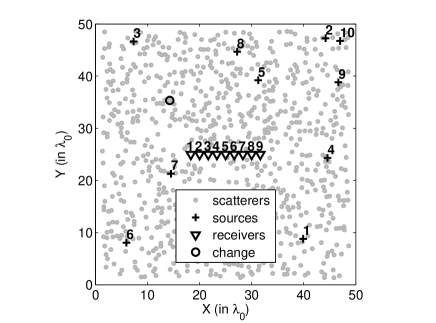
Figure 1: Distribution of sources, receivers, scatterers in the numerical simulation. The scatterer to remove is surrounded in gray.

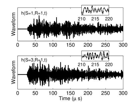
Figure 2: Normalized waveforms $h(t)$ obtained at receiver 1, for source number 1 (top) and 3 (bottom). Inset: zoom into the coda. The black solid (resp gray broken) line corresponds to the record acquired before (resp. after) the change. For illustration purpose, the value of $T_{0}$ was set to $1\,\mathrm{\mu s}$.

Parameter	notation	value
Number of scatterers		800
Transport mean free path	$\ell^{\star}$	$2.8\lambda_{0}$
	$k\ell^{\star}$	18
Diffusion constant	$D$	$1.4\,\lambda_{0}^{2}/T_{0}$
Thouless time	$\tau_{D}$	$68\,T_{0}$
Coda decay time (leakage)	$\tau_{\sigma}$	$240\,T_{0}$

Table 1: Physical parameters of the simulations in normalized units.

The signal $e(t)$ emitted by each source is a pulse with central frequency $f_{0}$ and a Gaussian envelope (100% bandwitdh at -6dB). Using source $i$ we record with receiver $j$ the signal $h_{ij}(t)$ during $300$ oscillations of period $T_{0}$. Typical waveforms $h_{ij}(t)$ are plotted in Fig. 2. The long tail of the record in Fig. 2 corresponds to arrival of partial waves that have been scattered several times. Notice that the ballistic arrival is not distinguishable in the waveforms of Figure 2. Long coda and lack of ballistic arrival constitute evidences that we are in a strongly scattering regime, in agreement with our estimates of the transport mean free path. During the first run of the simulation, $10\times 9$ impulse responses $h_{ij}$ are recorded and stored. On a second run, one scatterer is removed and another set of impulse responses $h^{\prime}_{ij}$ is evaluated. Both $h_{ij}(t)$ and $h^{\prime}_{ij}(t)$ display long codas lasting a large number of ballistic times.

II.2 Detection of an isolated change

The details of the complex waveforms shown in Figure 2 are highly sensitive to the positions of the the scatterers. Each waveform can be understood as a fingerprint of the medium. As our goal is to detect a single scatterer’s change, we need to exploit the information contained in both the amplitude and phase of the signals. A comparison of the records $h_{ij}(t)$ and $h^{\prime}_{ij}(t)$ reveals that for short coda times up to $100\,T_{0}\approx 30\tau^{*}$, no difference is visible in the signals. We observe small differences between the waveforms at later times that are solely due to the change in the medium. Figure 2 (bottom) shows an example of such differences for $h_{3,1}(t)$ and $h^{\prime}_{3,1}(t)$. The observed decorrelation is too large to be attributed to numerical noise, there is thus evidence that the coda waveforms are sensitive to the removal of only one scatterer.

The differences between the waveforms $h_{ij}$ and $h^{\prime}_{ij}$ are quantified by the decorrelation, or correlation loss, between $h_{ij}$ and $h^{\prime}_{ij}$. The decorrelation is computed in a time window of duration $2T$ centered on $t$ using the formula:

$$K_{ij}(t)=1-\frac{\int_{t-T}^{t+T}h_{ij}(u)\,h^{\prime}_{ij}(u){\mathrm{d}}u}{\sqrt{\int_{t-T}^{t+T}h_{ij}(u)^{2}{\mathrm{d}}u\int_{t-T}^{t+T}h^{\prime}_{ij}(u^{\prime})^{2}{\mathrm{d}}{u^{\prime}}}}.$$ (1)

The typical width of the time window $T$ is of the order of $5T_{0}$. Experimentally, enlarging $T$ partly eliminates the effect of noise and reduces the fluctuations of the correlation coefficient. Nonetheless, using a large value for $T$ results in considering simultaneously paths with very different lengths. We address this important point in Section III.2.

II.3 Spatial dependence of the decorrelation

In Figure 2, it is noticeable that the differences between $h_{1,1}(t)$ and $h^{\prime}_{1,1}(t)$ (top), are much smaller than the differences between $h_{3,1}(t)$ and $h^{\prime}_{3,1}(t)$ (bottom), even in the late coda. The decorrelations computed over the interval $[210\,T_{0},\,220\,T_{0}]$ are $K_{1,1}(215\,T_{0})=5\%$ and $K_{3,1}(215\,T_{0})=27\%$, respectively. Consequently, the amount of decorrelation depends on the positions of the source and receiver with respect to the local change, a property which holds even in very late time windows in the coda. For a given configuration of source-receiver pairs, we obtain a set of observed decorrelations, which are characteristic of the relative locations of the source, receiver and change in the multiple scattering medium. We will now demonstrate the possibility to locate the change and estimate its cross-section from the knowledge of the source and receiver positions and the corresponding decorrelation coefficients. To do so, we develop a theoretical model to predict the decorrelation coefficient of waves induced by the addition of a change in a heterogeneous medium, in the diffusive regime. We recall in the next section the necessary elements from multiple scattering theory.

III Wave scattering theory

We assume that the medium can be represented as a matrix with embedded inclusions. Only the scalar case is considered here. The scattering properties of an inclusion will be described by its $\mathcal{T}$ matrix, defined in operator notation as Sheng (2006); Economou (2006):

$$G_{1}=G_{0}+G_{0}\mathcal{T}G_{0}$$ (2)

where $G_{0}$ is the retarded free space Green function and $G_{1}$ is the Green function in the presence of the scatterer. For a non absorbing scatterer, energy conservation implies the following optical theorem:

$$-\frac{\Im\mathcal{T}(\omega)}{k_{0}}=\sigma(\omega),$$ (3)

where $\sigma$ is the scatterer cross-section.

III.1 Correlations between two slightly different media

We want to predict the decorrelation of waveforms in a medium where a small change occurs. Although we will employ a statistical approach based on ensemble averages, in general we have access to only one realization of the random process. Therefore we introduce the following estimator of the cross-correlation function based on the observation of a single coda:

$$\Gamma(t,\,\tau)=\frac{1}{2T}\int_{t-T}^{t+T}\psi^{2}(t^{\prime}+\tau/2)\psi^{1}(t^{\prime}-\tau/2){\mathrm{d}}{t^{\prime}},$$ (4)

where $\psi$ is the scalar field. The superscript $2$ refers to the medium in presence of an extra defect while the superscript $1$ refers to the medium without it. We have introduced an analog of the Wigner function which is most convenient to analyze non-stationary signals. The empirical cross-correlation can be decomposed over internal and external frequencies $\omega$ and $\Omega$, respectively:

$$\Gamma(t,\,\tau)=\frac{1}{(2\pi)^{2}}\int_{-\infty}^{\infty}{\mathrm{d}}\Omega\int_{-\infty}^{\infty}{\mathrm{d}}\omega\tilde{\Gamma}(\Omega,\,\omega)\,\exp[-\mathrm{i}(\Omega t+\omega\tau)]$$ (5)

where the frequency-domain cross-correlation reads:

$$\tilde{\Gamma}(\Omega,\,\omega)=\operatorname{sinc}(\Omega T)\,\psi^{2}(\omega+\Omega/2)\psi^{1}(\omega-\Omega/2)^{*}.$$ (6)

We see that the width of the time window, $2T$, has a minor effect only. Equation (6) shows that we have to compute the quantity

$$\left\langle{G^{2}(\omega+\Omega/2)G^{1}(\omega-\Omega/2)^{*}}\right\rangle.$$ (7)

In equation (7), $G$ is the retarded Green’s function. We will denote by $\mathcal{T}_{0}$ the $\mathcal{T}$-matrix of the additional defect which is assumed to appear at the position $\mathbf{x}_{0}$. In diagrammatic notations, such as the one employed in Figure 3 , the $\mathcal{T}$ matrices are represented by crosses. The transport of energy in the scattering medium is described by the ladder operator $L$, which is defined by the diagrammatic self-consistent equation shown in Figure 3 Sheng (2006); Akkermans and Montambaux (2007).

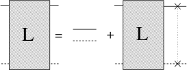
Figure 3: The Bethe-Salpeter equation defining the so-called ladder operator $L$. The solid line and dashed line represent the retarded ensemble averaged Green’s function and its complex conjugate, respectively. The dotted line connecting the two vertices indicates that they represent the same scatterer.

We use the field-field correlation function in the coda

$$\tilde{\Gamma}(\omega,\,\Omega,\,\mathbf{s},\,\mathbf{x}_{0},\,\mathbf{r})=\int{\mathrm{d}}{\mathbf{r}_{1}}\int{\mathrm{d}}{\mathbf{r}_{2}}\,\tilde{P}_{0}(\omega,\,\Omega,\,\mathbf{s},\,\mathbf{r}_{1})\\ \times\tilde{L}_{e}(\omega,\,\Omega,\,\mathbf{r}_{1},\,\mathbf{x}_{0},\,\mathbf{r}_{2})\tilde{P}_{0}(\omega,\,\Omega,\,\mathbf{r}_{2},\,\mathbf{r}).$$ (8)

Quantities labelled with ~ are implicitely evaluated at inner frequency $\omega$ and outer frequency $\Omega$. The ladder propagator $L_{e}$ describes the transport of correlations in a sequence of scattering events in the medium with an extra scatterer. $\tilde{P}_{0}(\mathbf{s},\,\mathbf{r}_{1})$ and $\tilde{P}_{0}(\mathbf{r}_{2},\,\mathbf{r})$ describe the ballistic propagation from the source to the first scattering event, and from the last scattering event to the detector, respectively:

$$\tilde{P}_{0}(\mathbf{r}_{1},\,\mathbf{r}_{2})=\frac{\mathrm{e}^{-R/\ell}}{(4\pi R)^{2}}\,\mathrm{e}^{\mathrm{i}\Omega R/c}$$ (9)

where $R=|\mathbf{r}_{2}-\mathbf{r}_{1}|$ and $c=\partial_{\omega}k_{0}(\omega)$ is the group velocity at the frequency $\omega$. The ladder propagator with the extra-scatterer $L_{e}$ is related to the ladder propagator without the extra-scatterer $L$ as follows Nieuwenhuizen and van Rossum M. C. W. (1993):

Figure 4: The diagram of the ladder operator with an extra scatterer. The extra scatterer is sandwiched between two ladder operators. Note that we have neglected the possibility that ensemble averaged Green’s functions connect the extra scatterer with the source and/or the receiver which assumes that it is located at least one mean free path away from all sources and receivers.

$$L_{e}(\mathbf{s},\,\mathbf{x}_{0},\,\mathbf{r})=L(\mathbf{s},\,\mathbf{r})+\\ \int\!\!{\mathrm{d}}{\mathbf{r}_{1}}\int\!\!{\mathrm{d}}{\mathbf{r}_{2}}L(\mathbf{s},\,\mathbf{r}_{1})J(\mathbf{r}_{1},\,\mathbf{x}_{0},\,\mathbf{r}_{2})L(\mathbf{r}_{2},\,\mathbf{r}).$$ (10)

In Equation (10), also represented by the diagram depicted in Figure 4, the first term represents the scattering paths that do not see the defect, while the second term describes the paths that visit the defect once. As we are in a regime of weak interaction between the field and the scatterer higher-order terms can be neglected. We define the operator $J$ that connects the two ladders by

$$J(\mathbf{r},\,\mathbf{x}_{0},\,\mathbf{r}^{\prime})=\\ \int\!\!{\mathrm{d}}{\mathbf{r}_{1}}\int\!\!{\mathrm{d}}{\mathbf{r}_{2}}\,G(\mathbf{r},\,\mathbf{r}_{1})\mathcal{T}(\mathbf{r}_{1},\,\mathbf{r}_{2})G(\mathbf{r}_{2},\,\mathbf{r}^{\prime})G(\mathbf{r},\,\mathbf{r}^{\prime})^{*},$$ (11)

where $G$ denotes the ensemble averaged Green’s function. In the mesoscopic regime, $J$ is evaluated to lowest order of the small quantity $1/(k_{0}\ell)\ll 1$ for a point scatterer:

$$J(\mathbf{r},\,\mathbf{x}_{0},\,\mathbf{r}^{\prime})\simeq-\frac{\mathrm{i}\ell^{2}\mathcal{T}_{0}}{8\pi k_{0}}\delta^{(3)}(\mathbf{r}-\mathbf{x}_{0})\delta^{(3)}(\mathbf{x}_{0}-\mathbf{r}^{\prime}).$$ (12)

Inserting expression (12) into equation (8) one obtains:

$$\tilde{\Gamma}(\mathbf{s},\,\mathbf{x}_{0},\,\mathbf{r})=\int{\mathrm{d}}{\mathbf{r}_{1}}\int{\mathrm{d}}{\mathbf{r}_{2}}\tilde{P}_{0}(\mathbf{s},\,\mathbf{r}_{1})L(\mathbf{r}_{1},\,\mathbf{r}_{2})\tilde{P}_{0}(\mathbf{r}_{2},\,\mathbf{r})\\ -\int{\mathrm{d}}{\mathbf{r}_{1}}\int{\mathrm{d}}{\mathbf{r}_{2}}\tilde{P}_{0}(\mathbf{s},\,\mathbf{r}_{1})\tilde{L}(\mathbf{r}_{1},\,\mathbf{x}_{0})\frac{\mathrm{i}\ell^{2}\mathcal{T}_{0}}{8\pi k}\tilde{L}(\mathbf{x}_{0},\,\mathbf{r}_{2})\tilde{P}_{0}(\mathbf{r}_{2},\,\mathbf{r}),$$ (13)

where the first term is the diffuse intensity in the medium without extra scatterer and the second integral is an interference term caused by the extra scatterer. In the slowly-varying envelope approximation, the integrals can be evaluated to give:

$$\tilde{\Gamma}(\mathbf{s},\,\mathbf{x}_{0},\,\mathbf{r})=\frac{\ell^{2}}{4\pi^{2}}\tilde{L}(\mathbf{s},\,\mathbf{r})-\frac{\ell^{2}}{4\pi^{2}}\tilde{L}(\mathbf{s},\,\mathbf{x}_{0})\frac{\mathrm{i}\ell^{2}\mathcal{T}_{0}}{8\pi k_{0}}\tilde{L}(\mathbf{x}_{0},\,\mathbf{r}).$$ (14)

In the diffusive regime, the propagator of the wave intensity in the medium filled with scatterers, $\tilde{P}_{d}$, is the solution of the following equation

$$\left(-\mathrm{i}\Omega-D\nabla^{2}_{\mathbf{r}_{2}}\right)\tilde{P}_{d}(\mathbf{r}_{1},\,\mathbf{r}_{2})=\delta^{(3)}(\mathbf{r}_{1}-\mathbf{r}_{2}),$$ (15)

where $D$ is the diffusivity. The ladder $L$ is related to $\tilde{P}_{d}$ by $\tilde{L}(\mathbf{r}_{1},\,\mathbf{r}_{2})=\frac{4\pi c}{\ell^{2}}\tilde{P}_{d}(\mathbf{r}_{1},\,\mathbf{r}_{2}).$ Using these notation the diffuse intensity for a unit point source satisfies:

$$\tilde{\Gamma}(\mathbf{s},\,\mathbf{x}_{0},\,\mathbf{r})=\frac{c}{4\pi}\tilde{P}_{d}(\mathbf{s},\,\mathbf{r})+\frac{c}{4\pi}\tilde{P}_{d}(\mathbf{s},\,\mathbf{x}_{0})\frac{\mathrm{i}c\mathcal{T}_{0}}{2k_{0}}\tilde{P}_{d}(\mathbf{x}_{0},\,\mathbf{r}).$$ (16)

In order to obtain the correlation function in the time domain, we double invert the Fourier transform over the variables $\omega$ and $\Omega$. We further assume that the signal has been filtered in a narrow frequency band $\Delta\omega$ in which the scattering properties vary little. Upon integration over $\omega$ and application of the optical theorem (3), the correlation function for a unit point-source normalized by the bandwidth $\Delta\omega$ reads:

$$\Gamma(\mathbf{s},\,\mathbf{x}_{0},\,\mathbf{r},\,t)=P_{d}(\mathbf{s},\,\mathbf{r},\,t)\\ -\frac{c\sigma}{2}\int_{0}^{t}{\mathrm{d}}u\,P_{d}(\mathbf{s},\,\mathbf{x}_{0},\,u)P_{d}(\mathbf{x}_{0},\,\mathbf{r},\,t-u).$$ (17)

We have therefore obtained the theoretical decorrelation $K(\mathbf{x}_{0},t)=\frac{c\sigma}{2}Q(\mathbf{s},\,\mathbf{x}_{0},\,\mathbf{r},\,t)$, where

$$Q(\mathbf{s},\,\mathbf{x}_{0},\,\mathbf{r},\,t)=\frac{\int_{0}^{t}{\mathrm{d}}u\,P_{d}(\mathbf{s},\,\mathbf{x}_{0},\,u)P_{d}(\mathbf{x}_{0},\,\mathbf{r},\,t-u)}{P_{d}(\mathbf{s},\,\mathbf{r},\,t)}.$$ (18)

The negative sign in (17) comes from the optical theorem (energy conservation) and ensures that the cross-coherence is less than one. The derivation presented in this section does not depend on the form of Equation (15), which means that solutions to a more accurate transport equation can be substituted to $P_{d}$. Note that for a resonant point scatterer, $\sigma$ can be substituted with $\lambda_{0}^{2}/\pi$.

III.2 Computation of the decorrelation formula

We observe that the decorrelation (18) can be computed if the function $P_{d}$ is known. In the general case where the diffusivity $D$ depends on the position, the function $P_{d}$ can only be numerically estimated, provided that the spatial dependence of $D$ is known. In practice, the decorrelation coefficient can be reasonably rapidly computed if one assumes that the value of $D$ is approximately uniform in the medium. We investigate the amount of variation for $D$ in Section IV.5.

If the medium is absorbing, the same issue arises. In media with a uniform absorption time $\kappa^{-1}$, the absorption affects the numerator of $Q$ in (18) by a factor $\exp[-\kappa u-\kappa(t-u)]=\exp[-\kappa t]$ and the denominator by a factor $\exp[-\kappa t]$. Therefore, uniform absorption effects cancel out in the normalized decorrelation function, which is a genuine advantage of the present technique. In the case where absorption is non-uniform, it will affect differently $P_{d}(\mathbf{s},\,\mathbf{x}_{0})$ and $P_{d}(\mathbf{x}_{0},\,\mathbf{r})$ and the observed decorrelation pattern may be partly ascribed to the spatial variations of absorption. Consider a medium with constant diffusivity $D$ and absorption $\kappa$. The solution of the diffusion equation (15) in an infinite $d$-dimensional medium is

$$P_{d}(\mathbf{r}_{1},\,\mathbf{r}_{2},\,t)=\frac{1}{(4\pi Dt)^{d/2}}\exp\left[-\kappa t-\frac{(\mathbf{r}_{2}-\mathbf{r}_{1})^{2}}{4Dt}\right].$$ (19)

In the case of a 3-D infinite medium, a usual Laplace transform calculation gives the exact result:

$$Q(\mathbf{s},\,\mathbf{x},\,\mathbf{r},\,t)=\frac{1}{4\pi D}\left(\frac{1}{s}+\frac{1}{r}\right)\exp\left[\frac{R^{2}-(s+r)^{2}}{4Dt}\right].$$ (20)

where we have introduce the notations $s=\|\mathbf{s}-\mathbf{x}\|$, $r=\|\mathbf{r}-\mathbf{x}\|$ and $R=\|\mathbf{s}-\mathbf{r}\|$. We observe that $Q$ is a function with elliptic contour lines multiplied by simple poles located at $\mathbf{s}$ and $\mathbf{r}$. Of course, if $\mathbf{r}=\mathbf{s}$, we recover the formula derived in Ref. Snieder et al. (2002) for an infinite medium. This formula is generally not applicable under this form because the transducers are usually located at the surface of the system. However, if the boundary conditions are sufficiently simple, the formula (20) can be used as a building block to derive more complicated solutions, as shown in Section V.

In formula (17) we neglect two constraints. First, we assume that the change occurs at a minimum distance of the order of one mean free path from the source and the receiver. Second, we neglect the finite velocity of the wave, in other words, the contribution for times $u,t-u<R/c$ in the integral (17) should be removed. The contribution of short times $u<R/c$ in (17) is negligible as soon as $ct\gg R>\ell^{\star}$. The computation of the decorrelation coefficients $K_{ij}(t)$ must be done with $T$ larger than a few oscillation periods of the wave. Using formula (20), we can estimate the correction due to this averaging as a function of $T/t$. To do so, we compute the average of (20) on the interval $[t-T,\,t+T]$ and divide by the value of $Q$ at $t$. We obtain a curve of relative correction as a function of $T/t$ which is independent of any other parameters and which is displayed on Figure 5. In most applications, the correction will be typically less than 10%.

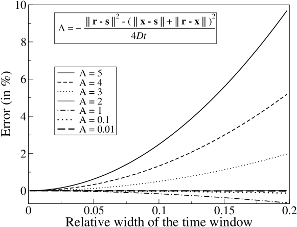
Figure 5: Deviation of the average of $Q$ on the time interval $[t-T,\,t+T]$ with repect to $Q(t)$. The correction grows more rapidly for large values of the argument in the exponential of (20), denoted by A in this Figure.

III.3 Intensity variations vs field correlations

As recalled in the introduction, a number of investigations on the monitoring of complex media have focused on the detection of intensity variations induced by local changes of the scattering properties. We will show that in the diffusive regime, intensity variations are much less sensitive to local changes than field correlations. To do so, we calculate the perturbation of the ladder propagator induced by an extra-scatterer following the approach developed in reference Nieuwenhuizen and van Rossum M. C. W. (1993). In addition to the diagram depicted in Figure 4, two other diagrams contribute to intensity variations: 1) a diagram with a single cross on the lower line and 2) a diagram with one cross on each line which are connected by dashed line. In the diffusive regime and for a non-absorbing defect, we obtain the intensity perturbation to lowest-order in $\mathbf{q}$ and $\mathbf{q}^{\prime}$ in the form:

$$\delta L_{e}^{I}(\mathbf{s},\,\mathbf{x},\,\mathbf{r};\,t)=\frac{\ell^{4}\mathcal{T}\mathcal{T}^{\star}}{48\pi^{2}}\int^{+\infty}_{-\infty}\frac{{\mathrm{d}}\Omega}{2\pi}\iiint_{\mathbb{R}^{3}\times\mathbb{R}^{3}}{\mathrm{d}}^{3}\mathbf{q}\,{\mathrm{d}}^{3}\mathbf{q}^{\prime}\\ L(\mathbf{q};\Omega)\mathrm{e}^{\mathrm{i}\mathbf{q}\cdot(\mathbf{r}-\mathbf{x})}(\mathbf{q}\cdot\mathbf{q}^{\prime})L(\mathbf{q}^{\prime};\,\Omega)\mathrm{e}^{\mathrm{i}\mathbf{q}^{\prime}\cdot(\mathbf{x}-\mathbf{s})}\mathrm{e}^{-\mathrm{i}\Omega t}.$$ (21)

In the Fourier domain, the ladder propagator in the diffusion regime writes:

$$L(\mathbf{q};\,\Omega)=\dfrac{4\pi}{(2\pi)^{3}\ell^{2}\left(q^{2}\ell/3-\mathrm{i}\Omega/c\right)}.$$ (22)

After integration over the wavenumbers $\mathbf{q}$, $\mathbf{q}^{\prime}$ and the frequency $\Omega$, we obtain:

$$\delta L_{e}^{I}(\mathbf{s},\,\mathbf{x},\,\mathbf{r};\,t)=\dfrac{\sigma c}{6\pi^{1/2}D^{3/2}t^{3/2}}\mathrm{e}^{-R^{2}/4Dt}\times\\ \nabla_{\mathbf{s}}\cdot\;\left(\nabla_{\mathbf{r}}Q(\mathbf{s},\,\mathbf{x},\,\mathbf{r})\right).$$ (23)

After calculation of the partial derivatives, we obtain the following formula for the ladder perturbation induced by an extra scatterer:

$$\delta L_{e}^{I}(\mathbf{s},\,\mathbf{x},\,\mathbf{r};t)=\dfrac{\sigma c^{2}(\mathbf{r}-\mathbf{x})\cdot(\mathbf{s}-\mathbf{x})}{48\pi^{3/2}D^{7/2}t^{5/2}r^{2}s^{2}}\times\\ \left(\dfrac{r^{3}+s^{3}}{rs}+\dfrac{(r+s)^{3}}{2Dt}\right)e^{-(r+s)^{2}/4Dt}$$ (24)

The intensity variation exhibits a characteristic pattern with positive and negative lobes, depending on the cosine of the angle between the source and receiver as seen from the additional scatterer. Even more important is the temporal dependence $t^{-5/2}$ which is faster than the temporal decay of the ladder propagator between the source and receiver. As a consequence, the sensitivity to the local change decays like $1/t$ in the coda in sharp contrat to the field correlation which goes to a constant at large lapse time. This property justifies the popular use of field correlation functions to monitor temporal changes in evolving media.

IV The inversion technique

IV.1 Maximum likelihood of the position

In Section III, we have obtained an expression for the expected decorrelation as a function of the position of the change. The principle of the inversion technique is to compare a numerical model to experimental data. The change is found at the position where numerical and experimental decorrelation match best. The mismatch is measured by a standard least-squares cost function ($\chi^{2}$). The inversion technique consists in finding the position $\mathbf{x}$ and the cross-section $\sigma$ minimizing the function $\chi^{2}$. Such a technique is also often called a maximum likelihood method. Let us chose a set of sources $\mathbf{s}_{i}$ ($1\leq i\leq n_{s}$) and a set of receivers $\mathbf{r}_{j}$ ($1\leq j\leq n_{r}$), and call $N$ the number of source-receiver pairs (in this case, $N=n_{r}n_{s}$). There is no restriction on their positions, and in particular source and receiver can be located at the same position. We describe the technique at fixed time $t$ in the coda.

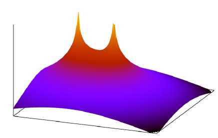
Figure 6: The function $Q_{ij}(\mathbf{x})$ in a infinite medium in dimension 3 with constant diffusivity and absorption computed with formula (20). The function is plotted in the plan containing the source, the receiver and the change. The value along the $z$ axis (logarithmic) is the sensitivity to a change at the position in $(x,y)$. The two peaks correspond to the positions of the source and the receiver. The $z$-scale is logarithmic and arbitrary.

The most restrictive assumption of our approach is that a single defect affects the experimental values of the decorrelation. The LOCADIFF inversion technique consists in retrieving the most likely position of this defect by introducing the cost function:

$$e(\mathbf{x})=\sum_{i,j}\left(K^{m}_{ij}(t)\right.-K_{ij}(\mathbf{x},\,t))^{2}/\epsilon^{2},$$ (25)

where $K^{m}_{ij}(t)$ denotes the experimental measurements of the decorrelation and the coefficients $K_{ij}(\mathbf{x},\,t)$ are the theoretical decorrelations assuming that the defect is located at $\mathbf{x}$. The typical fluctuations on the measured decorrelations are encapsulated in the parameter $\epsilon$.

To find the value of the scattering cross-section $\sigma$, also unknown, we remark that $e(\mathbf{x})$ is, as a function of $\sigma$, a polynomial of degree two. There is therefore a minimum depending on $\mathbf{x}$ at

$$\sigma_{\text{opt}}(\mathbf{x})=\frac{2}{c}\frac{\sum_{i,j}K^{m}_{ij}(t)Q_{ij}(\mathbf{x},\,t)}{\sum_{i,j}Q_{ij}(\mathbf{x},\,t)^{2}}.$$ (26)

We reintroduce the value of $\sigma_{\text{opt}}$ into the expression (25) and get the optimized error function

$$e_{\text{opt}}(\mathbf{x})=\sum_{i,j}\dfrac{K_{ij}(t)^{2}}{\epsilon^{2}}-\frac{\left(\sum_{i,j}K_{ij}(t)Q_{ij}(\mathbf{x},\,t)\right)^{2}}{\epsilon^{2}\sum_{i,j}Q_{ij}(\mathbf{x},\,t)^{2}}$$ (27)

which does not depend on $\sigma$ anymore. The most likely position of the defect is the position $\mathbf{x}_{0}$ of the minimum of $e_{\text{opt}}$. The value of the cross-section is $\sigma_{\text{opt}}(\mathbf{x}_{0})$ obtained from Equation (26).

To give an interpretation to the values of $e(\mathbf{x})$, it is customary to normalize it in the following way

$$\chi^{2}_{n}(\mathbf{x})=\frac{e(\mathbf{x})}{f}$$ (28)

where $f=N-4$ is the number of degrees of freedom, since four model parameters -the cross-section and the cartesian coordinates of the defect- are to be estimated. The quantity $\chi^{2}_{n}(\mathbf{x})$ has the following interpretations. If $\chi^{2}_{n}(\mathbf{x})\gg 1$, it is very unlikely that the point $\mathbf{x}_{0}$ is actually located at $\mathbf{x}$. If $\chi^{2}_{n}(\mathbf{x})\simeq 1$ the point $\mathbf{x}$ is a good candidate for $\mathbf{x}_{0}$. If $\chi^{2}_{n}(\mathbf{x}_{0})\ll 1$, there is a large area where $\chi^{2}_{n}(\mathbf{x})<1$ which means that the inversion could not locate precisely the change because the value of $\epsilon$ is too large. In other words the quality of measurements is too poor to give any satisfactory result. It is possible to use $\chi^{2}_{n}(\mathbf{x})$ to obtain the probability density that the defect has appeared at the point $\mathbf{x}$, which we define as:

$$p(\mathbf{x})=\frac{1}{C}\exp\left[-\frac{1}{2}N\chi^{2}_{n}(\mathbf{x})\right]=\frac{1}{C}\exp\left[-\frac{e(\mathbf{x})}{2\epsilon^{2}}\right]$$ (29)

where $C$ is a normalization constant such that $\int p(\mathbf{x}){\mathrm{d}}\mathbf{x}=1$ (see the appendix for a derivation of this formula).

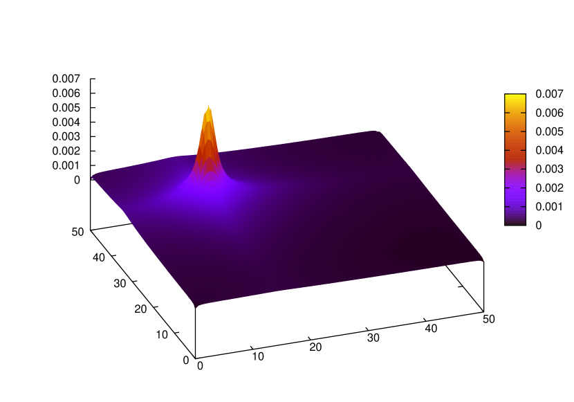
Figure 7: Density of probability for the position of the moving scatterer.

IV.2 Resolution versus number of source-receiver pairs

To investigate the resolution of the inversion technique depending on the parameters of the likelihood maximization, we use a numerical approach. We compute the best achievable resolution regardless of all experimental difficulties that potentially degrade the accuracy of the location. We use an ideal set-up made of one source and $N$ receivers regularly distributed on a circle (see figure 8). We introduce a change at the center of the circle by adding a single scatterer with cross-section $\sigma$. For each pair of receiver, we compute synthetic data through application of the formula (20). The Thouless time $\tau_{D}$ is defined as $L^{2}/D$. As a measure of the precision, a resolution length $\delta$ is introduced, which we compute using the probability density function (29) as follows: $\delta^{2}=\int(\mathbf{x}-\mathbf{x}_{0})^{2}p(\mathbf{x}){\mathrm{d}}\mathbf{x}$.

In the vicinity of the change, we infer that the contributions of the terms in $e(\mathbf{x})$ are comparable and we deduce that $\delta\propto\epsilon$. Thus, the precision with which the measurements are made directly influences the precision with which the change is located. We will not study the dependence of $\delta$ with respect to $\epsilon$ and we chose a value $\epsilon=0.01$ throughout the numerical study. Note that a uniform probability distribution corresponds to a complete absence of information concerning the location of the change, and gives the value $\delta\simeq L$. The typical behaviour of the resolution $\delta$ as a function of the number of source-receiver pairs is depicted in Figure 9. In the configuration described above, each pair gives a comparable contribution to $e(\mathbf{x})$ so that $e(\mathbf{x})$ is approximately proportional to $N$. Therefore in the ideal case described in our example, we find that $\delta\propto N^{-1/2}$.

Note that the resolution cannot be made arbitrarily small by increasing $N$ at will, because it is not possible to find an arbitrary number of source-receiver pairs providing independent data. The value $N$ entering into the scaling law $\delta\propto N^{-1/2}$ is the number of independent decorrelation measurements.

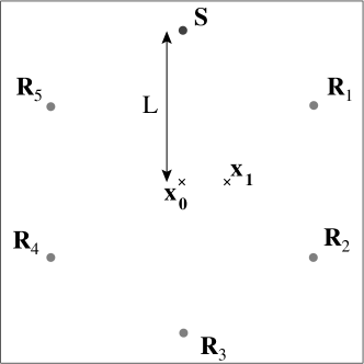
Figure 8: Description of the numerical setup used for investigating the accuracy of the inversion technique. The example is shown with $N=5$. The other parameters of the numerical simulations are : $L=10$, $D=1$, $c=1$. The change $\mathbf{x}_{0}$ is located at the center of the circle and is used in Section IV.2 to study the optimal spatial resolution of the inversion. The change located at point $\mathbf{x}_{1}$ is used to study the robustness of the inversion technique against measurement errors on the determination of $D$ in Section IV.5.

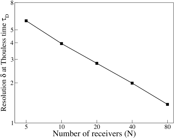
Figure 9: Spatial resolution at the coda time $t=\tau_{D}$, as a function of the number of receivers, where $\tau_{D}$ is the Thouless time. The typical setup for the numerical experiment is depicted in Figure 8. The dots correspond to the values of the resolution for $N=5$, $10$, $20$, $40$ and $80$. The double logarithmic scale provides clear evidence of the relation $\delta\sim N^{-1/2}$.

IV.3 Resolution versus coda time

The dependence of the resolution $\delta$ with respect to coda time, is shown on Figure 10 for $\sigma=1$, $D=1$, $c=1$, $L=10$ and $\epsilon=0.01$. The resolution exhibits a minimum at a time of order $t_{\rm min}=\tau_{D}$. For a given source-receiver pair, the coda time is the time that has elapsed after the arrival of the ballistic wave. Shortly after the ballistic arrival, the waves that reach the receiver have followed “snake-like” paths around the direct ray. In the early coda, the only signals sensitive to the change are those for which the change is located along the segment joining the source and the receiver. Later in the coda, the diffuse waves arriving at the receiver have explored a larger volume of the system. This qualitatively explains why $\delta$ decreases with the coda time $t$. At very late times, the formula (20) reveals that the decorrelation for each source receiver pair saturates, as the exponential factor tends to $1$. The asymptotic spatial sensitivity to the change is algebraic only. After reaching a minimum, $\delta$ increases because the variations of $\chi^{2}_{n}$ with respect to $\mathbf{x}$ decreases. The minimum for $\delta$ is found approximately at time $\tau_{D}$, the Thouless time, after which the whole system has been explored by the diffuse waves and yet $Q$ still exhibits large spatial variations.

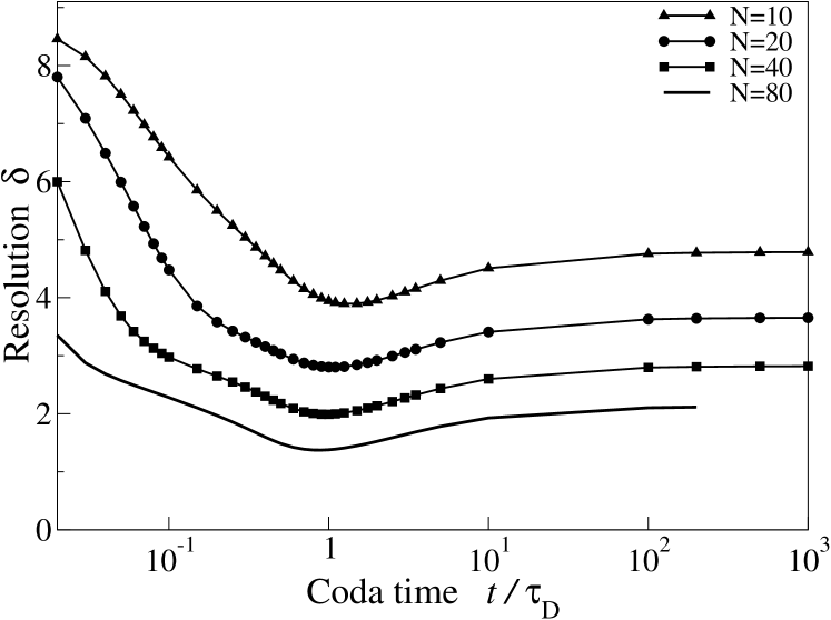
Figure 10: Spatial resolution obtained for the setup of Figure 8 for the values $N=5$, $10$, $20$, $40$ and $80$ and for coda times varying from $2.10^{-2}\tau_{D}$ to $10^{3}\tau_{D}$. The time scale is logarithmic. A minimum of the resolution is found at $t\simeq\tau_{D}$.

IV.4 Resolution versus cross-section

The scattering cross-section $\sigma$ of the change also influences the precision of the technique. We observe that the resolution $\delta$ decreases as $\sigma$ increases. Note that when $\sigma$ is very small, $\delta$ goes to a value $\sim L$, meaning that it is not possible to detect the change. When $\sigma\simeq L^{2}$, the cross-section is equivalent to the area of the system, and locating a change has no physical significance in this limit. In Figure 11 we plot the variations of $\delta$ at the optimal time $t=\tau_{D}$ as  $\sigma$ varies from $10^{-4}L^{2}$ to $L^{2}$. The other parameters of the calculations are $D=1$, $c=1$, $\epsilon=0.01$, $N=10$. We observe that the spatial resolution $\delta$ decreases by a factor 2 as the cross-section increases from $10^{-2}$ to 1.

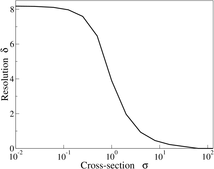
Figure 11: Optimal resolution $\delta$ as a function of the cross-section of the change $\sigma$ obtained for the setup of Figure 8. Other parameters of the simulations are $D=1$, $c=1$, $N=10$, $\epsilon=0.01$.

IV.5 Sensitivity to the value of the diffusivity $D$

Our inversion technique depends heavily upon our ability to estimate the diffusivity of the waves in the heterogeneous medium. Although the absorption time $\tau$ does not enter into the final formula (20), let us remark that in practice $D$ and $\tau$ cannot be measured independently. The diffusivity $D$ is the crucial physical parameter which enters into the formula for the intensity propagator $P_{d}$ and controls the accuracy of the energy propagation model of the medium. It is therefore important to quantify the impact of errors in the diffusivity $D$ on the accuracy of our method. Even if we use an incorrect value for the diffusivity, our inversion procedure still provides an answer for the position of the defect. The main issue is to quantify to what extent the inferred position differs from the exact location of the target. To address this point, we plot the spatial resolution and the absolute error of the inversion for a wide range of values of $D$ on a specific example.

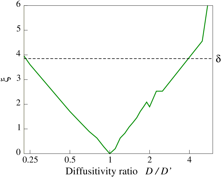
Figure 12: Effect of an estimation error on the value of the diffusivity $D$ induced on the relocation of a target. Synthetic data were calculated with $D=1$ and inverted with modified values of the diffusivity $D^{\prime}$ ranging from 0.2 to 8. The other parameters of the simulation are $\sigma=1$, $L=10$, $N=10$, $\epsilon=0.01$ and the change is located at the position $\mathbf{x}_{1}$ (see Figure 8). $\xi$ is the distance between $\mathbf{x}_{1}$ and the point where $\chi^{2}(\mathbf{x})$ is minimum. In the simulated configuration, the inversion technique remains accurate even if $D^{\prime}$ differs from $D$ by a factor $2$.

We use the approach described in Section IV.2. First, a synthetic data set is computed with a value $D$ for the diffusivity. This synthetic data set is then inverted for the location of the target using a different diffusivity $D^{\prime}$. The change is located at the position $\mathbf{x}_{1}$ indicated on Figure 8. The other physical parameters $L=10$, $\sigma=1$, $N=10$, $\epsilon=0.01$ and $t$ have been adjusted to provide the smallest spatial resolution $\delta$. We call $\xi$ the distance between the change located by the inversion and $\delta$ is the resolution length. The results of the simulation are displayed in Figure 12. It is rather remarkable that an error on  $D$ as large as a factor of $2$ yields a location of the change within one half of the resolution length. In this specific but realistic example, the inversion technique is therefore very robust against errors on the determination of $D$. This constitutes a major advantage of our method. Based on these results, we infer that spatial variations of $D$ within a factor of $2$ will not affect the results dramatically.

V Boundary conditions

The inversion technique presented in section IV.1 relies on the knowledge of the function $P_{d}$, the diffusion kernel, which depends on the boundary conditions of the system. For simplicity, we studied the LOCADIFF technique in an infinite medium without taking into account the effect of boundaries, which may not be realistic in applications. An abundant literature is dedicated to solving the diffusion equation in a wide range of situations Crank (1975). In many cases of practical interest, sophisticated techniques are required to provide an exact solution or a numerical approximation up to a required accuracy. In the infinite medium, the decorrelation (18) can be computed numerically. In the presence of boundaries, it is more difficult to compute the Green’s function because translational invariance is lost. However, if the boundaries are flat, it possible to construct the Green’s function from the solution without boundaries using symmetry arguments. In the general case, one has to solve the diffusion equation for the geometry of the system, which is a problem for applied mathematics in itself.

In the simple case of a single planar boundary, the solution $P^{B}_{d}$ of the diffusion equation of the semi-infinite medium, can be deduced from $P^{\infty}_{d}$, using the technique of images:

$$P^{B}_{d}(\mathbf{s},\,\mathbf{r},\,t)=\alpha\left(P_{d}(\mathbf{s},\,\mathbf{r},\,t)+\beta P_{d}(\mathbf{s}^{\prime},\,\mathbf{r},\,t)\right)$$ (30)

where $\mathbf{s}^{\prime}$ is the image of $\mathbf{s}$ with respect to the boundary (see Figure 13) and $\beta$ is a characteristic coefficient depending on the nature of the boundary condition. For instance if the boundary is absorbing, $\beta=-1$ and if it is fully reflecting, we have $\beta=1$. The normalization coefficient $\alpha$ is, in the case of constant diffusivity

$$\alpha^{-1}=\frac{1+\beta}{2}+\frac{1-\beta}{2}\operatorname{erf}\left(\frac{d_{B,\mathbf{s}}}{\sqrt{4Dt}}\right)$$ (31)

where $d_{B,\mathbf{s}}$ is the distance from the source to the boundary. Note that $\alpha$ is undetermined in the case where the conditions $\beta=-1$ and $d_{B,\mathbf{s}}=0$ are met simultaneously.

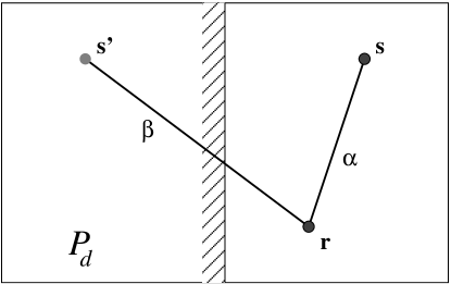
Figure 13: Schematic representation of a boundary condition for $P_{d}$. The image of the source $\mathbf{s}$ is noted $\mathbf{s}^{\prime}$ and the arbitrary point is $\mathbf{r}$. The solid line is the solution in the infinite medium.

The solution to the diffusion equation in presence of the boundary can be plugged into the decorrelation expression (18) leading to four terms (figure 14). Note that in case there are more boundaries, the image technique requires to take into account infinitely many images. Other techniques also lead to infinite series.

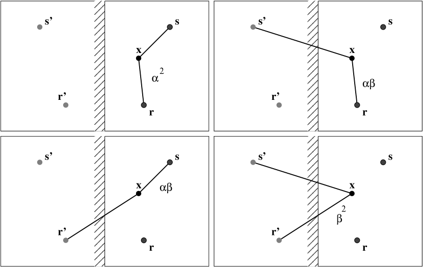
Figure 14: In presence of a single straight boundary, the decorrelation function (18) involves four terms, coming from the product of two formula of the form (30). We use the images of the source $\mathbf{s}$ and the receiver $\mathbf{r}$: Thanks to the symmetry of the diffusion equation, there is no need to introduce the image of the point $\mathbf{x}$.

VI Discussion

In this section, we discuss issues related to the practical use of the LOCADIFF technique as well as possible improvements. We first note that if the interval between the records of $h_{ij}$ and $h^{\prime}_{ij}$ is large, the medium may also have experienced a global change, for instance a dilation due to a temperature change. In this case, the computation of the decorrelation may be refined by taking into account a global relative velocity change $\epsilon$, where $\epsilon$ yields the maximum value of the correlation

$$\frac{\int h_{ij}((1+\epsilon)u)\,h^{\prime}_{ij}(u){\mathrm{d}}u}{\sqrt{\int h_{ij}(u)^{2}{\mathrm{d}}u\int h^{\prime}_{ij}(u^{\prime})^{2}{\mathrm{d}}{u^{\prime}}}}.$$ (32)

where the integrals are performed along the whole record Larose and Hall (2008).

Another issue concerns the possible improvements on the inversion procedure. Under the form presented in this article, the LOCADIFF technique only uses a small time window in the signals. It would be of great interest to take into account several time windows in the coda. This would provide more independent data for the inversion procedure and may reduce the effect of noise.

Finally, we point out that the kernel used in the inversion is computed from the solution to the diffusion equation. In some simple geometries, like the infinite medium, the solution is analytic and simple to compute. If the shape of the medium is irregular, with possibly more complicated boundary conditions, the kernels can only be approximated numerically. Alternatively, our approach could benefit from recent developpements in the implementation of the radiative transfer equation.

VII Conclusion

In this article, we have shown that it is possible to use the high sensitivity of diffuse waves to detect, characterize and locate a small change in a strongly scattering medium. Our technique uses the correlation of coda waveforms recorded before and after the change. Based on a maximum-likelihood approach, and a simple diffusion model, we demonstrate the possibility to retrieve the position of the change along with its scattering cross-section. We have also investigated the optimal values of the parameters that enter in the inversion procedure, based on a simple setup where sources and receivers are arranged on a circle surrounding the change. Three features have been identified: 1) We found that the resolution scales with the inverse square root of the number of sensors. 2) The technique provides the best results when the correlation window is centered on the Thouless time of the system. 3) We demonstrated that the technique is not very sensitive to errors in the measurement of the diffusivity.

Several aspects are still to be investigated. First, we have assumed that a single change occurs in the medium, an assumption which is probably too restrictive in some applications. In a straightforward generalization of our technique to $n$ changes, the dimension of the parameter space scales like $4n$ which in turn considerably increases the computation time. An alternative route for the inversion has to be found. Second, we have made the assumption of a point-like change. An extended change may not necessarily be equivalent to a collection of point-like changes. Again, an alternative approach to the inverse problem will be needed. We are currently investigating these two issues.

Using 2D finite difference wave simulations, we have demonstrated that LOCADIFF efficiently locates a small change in a multiple scattering environment. In a seperate paper Larose et al. (2010), experiments have also been conducted with ultrasound in concrete. The change was a hole drilled in the sample, and the LOCADIFF technique successfully retrieved its actual position. Other applications in geophysics and material sciences can be envisaged.

Appendix A Derivation using Bayesian inversion

We shortly derive here the density of probability density (29) using a Bayesian inference. In this calculation, we suppose that there is a change at an unknown position $\mathbf{x}$. The values of the measurements $K^{m}_{ij}$ are accurate up to an error order $\epsilon$ such that they are distributed around the numerical value $K_{ij}(\mathbf{x},t)$ according to a standard error function.

$$p(K^{m}_{ij}|\mathbf{x})=\frac{1}{\sqrt{2\pi}\epsilon}\exp\left[-\frac{(K_{ij}(\mathbf{x},\,t)-K^{m}_{ij})^{2}}{2\epsilon^{2}}\right].$$ (33)

Each pair $(i,j)$ provides an independent information. The Bayesian inversion consists in finding the probability density of $\mathbf{x}$ knowing the values of $K^{m}_{ij}$, namely to compute $p(\mathbf{x}|\{K^{m}_{ij}\})$. Let us call $p_{n}(\mathbf{x})$ the probability density for the position of the change when $n$ source-receiver pairs have been taken into account. Before measurement, the probability of the location of the change is uniform in the whole medium, so we have $p_{0}(\mathbf{x})=\frac{1}{V}$ ($V$ is the volume). Suppose we know $p_{n-1}(\mathbf{x})$ and let us compute the joint probability of $\mathbf{x}$ and $K_{n}$ using Bayes’ formula. We use the two relations:

$$p(\mathbf{x},K^{m}_{n}|K^{m}_{1},\dots\,K^{m}_{n-1}) =p_{n}(\mathbf{x})p(K^{m}_{n})$$ (34)

$$p(\mathbf{x},K^{m}_{n}|K^{m}_{1},\dots\,K^{m}_{n-1}) =p(K^{m}_{n}|\mathbf{x})p_{n-1}(\mathbf{x})$$ (35)

Integrating (34) over $\mathbf{x}$ we can compute $p(K^{m}_{n})$ as

$$\left(\int_{V}p_{n}(\mathbf{x}){\mathrm{d}}\mathbf{x}\right)p(K^{m}_{n})=\int_{V}p(\mathbf{x},\,K^{m}_{n}|K^{m}_{1},\,\dots K^{m}_{n-1}){\mathrm{d}}\mathbf{x}$$ (36)

The integral of $p_{n}(\mathbf{x})$ is equal to $1$ so we conclude that, using (35),

$$p_{n}(\mathbf{x})=\frac{p(K^{m}_{n}|\mathbf{x})p_{n-1}(\mathbf{x})}{\int_{V}p(K^{m}_{n}|\mathbf{x})p_{n-1}(\mathbf{x}){\mathrm{d}}\mathbf{x}}.$$ (37)

Therefore we have a recurrence scheme yielding the distribution of probability $p_{N}(\mathbf{x})$:

$$p_{N}(\mathbf{x})=\frac{\prod_{n=1}^{N}p(K^{m}_{n}|\mathbf{x})}{\int\prod_{n=1}^{N}p(K^{m}_{n}|\mathbf{x}){\mathrm{d}}\mathbf{x}}$$ (38)

which gives Equation (29) after replacing the probabilities with expression (33).

References

- Pine et al. (1988) D. J. Pine, D. A. Weitz, P. M. Chaikin, and E. Herbolzheimer, Phys. Rev. Lett., 60, 1134 (1988).
- Berkovits (1991) R. Berkovits, Phys. Rev. B, 43, 8638 (1991).
- Cowan et al. (2002) M. L. Cowan, I. P. Jones, J. H. Page, and D. A. Weitz, Phys. Rev. E, 65, 066605 (2002).
- Nieuwenhuizen and van Rossum M. C. W. (1993) T. M. Nieuwenhuizen and van Rossum M. C. W., Physica A, 177, 102 (1993).
- Feng and Sornette (1991) S. Feng and D. Sornette, J. Acoust. Soc. Am., 90, 1742 (1991).
- Vanneste et al. (1993) C. Vanneste, S. Feng, and D. Sornette, Europhys. Lett., 24, 339 (1993).
- den Outer et al. (1993) P. N. den Outer, T. M. Nieuwenhuizen, and A. Lagendijk, J. Opt. Soc. Am. A, 10, 1209 (1993).
- van Rossum and Nieuwenhuizen (1999) M. C. W. van Rossum and T. M. Nieuwenhuizen, Rev. Mod. Phys., 71, 313 (1999).
- Poupinet et al. (1984) G. Poupinet, W. Ellsworth, and J. Frechet, J. Geophys. Res, 89, 5719 (1984).
- Ratdomopurbo and Poupinet (1995) A. Ratdomopurbo and G. Poupinet, Geophys. Res. Lett, 22, 775 (1995).
- Cowan et al. (2000) M. L. Cowan, J. H. Page, and D. A. Weitz, Phys. Rev. Lett., 85, 453 (2000).
- Snieder et al. (2002) R. Snieder, A. Grêt, H. Douma, and J. Scales, Science, 295, 2253 (2002).
- Pacheco and Snieder (2005) C. Pacheco and R. Snieder, J. Acoust. Soc. Am., 118, 1300 (2005).
- Larose and Hall (2008) É. Larose and S. Hall, J. Acoust. Soc. Am., 125, 1853 (2008).
- Lobkis and Weaver (2003) O. I. Lobkis and R. L. Weaver, Phys. Rev. Lett., 90, 254302 (2003).
- Brenguier et al. (2008) F. Brenguier, M. Campillo, C. Hadziioannou, N. M. Shapiro, R. M. Nadeau, and É. Larose, Science, 321, 1478 (2008).
- Michaels and Michaels (2005) J. E. Michaels and T. E. Michaels, IEEE Trans. Ultrasonics, Ferroelectrics and Freq. Control, 52, 1769 (2005).
- Tremblay et al. (2010) N. Tremblay, É. Larose, and V. Rossetto, J. Acoust. Soc. Am. (2010).
- Snieder and Page (2007) R. Snieder and J. Page, Physics today, 60, 49 (2007).
- Poupinet et al. (2008) G. Poupinet, J.-L. Got, and F. Brenguier, “Earth heterogeneity and scattering effects on seismic waves,” (Academic Press, New York, 2008) Chap. Monitoring temporal variations of physical properties in the crust by cross-correlating the waveforms of seismic doublets, pp. 374–399.
- Derode et al. (2003) A. Derode, É. Larose, M. Tanter, J. de Rosny, A. Tourin, M. Campillo, and M. Fink, J. Acoust. Soc. Am., 113, 2973 (2003).
- Larose et al. (2006) É. Larose, L. Margerin, A. Derode, B. van Tiggelen, M. Campillo, N. Shapiro, A. Paul, L. Stehly, and M. Tanter, Geophysics, 71, SI11 (2006).
- Wapenaar et al. (2005) K. Wapenaar, J. Fokkema, and R. Snieder, J. Acoust. Soc. of Am., 118, 2783 (2005).
- Wapenaar et al. (2006) K. Wapenaar, E. Slob, and R. Snieder, Phys. Rev. Lett., 97, 234301 (2006).
- Gouédard et al. (2008) P. Gouédard, L. Stehly, F. Brenguier, M. Campillo, Y. de Verdiere, E. Larose, L. Margerin, P. Roux, F. Sanchez-Sesma, S. NM, and R. Weaver, Geophysical prospecting, 56, 375 (2008).
- Sens-Schönfelder and Wegler (2006) C. Sens-Schönfelder and U. Wegler, Geophys. Res. Lett., 33, L21302 (2006).
- Wegler and Sens-Schoenfelder (2007) U. Wegler and C. Sens-Schoenfelder, Geophys. J. Int., 168, 1029 (2007).
- Aubry and Derode (2009) A. Aubry and A. Derode, Phys. Rev. Lett., 102, 084301 (2009).
- Note (1) The code named ACEL has been developed by M. Tanter, Institut Langevin, Paris France. More details in http://www.institut-langevin.espci.fr/Mickael-Tanter,143.
- Sheng (2006) P. Sheng, Introduction to wave scattering localization and mesoscopic phenomena (Springer, Berlin, 2006).
- Economou (2006) E. N. Economou, Green’s Functions in Quantum Physics (Springer, Berlin, 2006).
- Akkermans and Montambaux (2007) E. Akkermans and G. Montambaux, Mesoscopic physics of electrons and photons (Cambridge Univ Press, 2007).
- Crank (1975) J. Crank, The mathematics of diffusion, 2nd ed. (Oxford, 1975).
- Larose et al. (2010) É. Larose, T. Planès, V. Rossetto, and L. Margerin, Appl. Phys. Lett., 96, 204101 (2010).