The Planck SZ Cluster Catalog: Expected X-ray Properties

Surveys based on the Sunyaev-Zel’dovich (SZ) effect provide a fresh view of the galaxy cluster population, one that is complementary to X-ray surveys. To better understand the relation between these two kinds of survey, we construct an empirical cluster model using scaling relations constrained by current X-ray and SZ data. We apply our model to predict the X-ray properties of the Planck  SZ Cluster Catalog (PCC) and compare them to existing X-ray cluster catalogs. We find that Planck  should significantly extend the depth of the previous all-sky cluster survey, performed in the early 1990s by the ROSAT satellite, and should be particularly effective at finding hot, massive clusters ($T>6\,\rm{keV}$) out to redshift unity. These are rare objects, and our findings suggest that Planck  could increase the observational sample at $z>0.6$ by an order of magnitude. This would open the way for detailed studies of massive clusters out to these higher redshifts. Specifically, we find that the majority of newly-detected Planck clusters should have X-ray fluxes $10^{-13}\,{\rm ergs/s/cm}^{2}<f_{X}[0.5-2\;{\rm keV}]<10^{-12}\,{\rm ergs/s/cm}^{2}$, i.e., distributed over the decade in flux just below the ROSAT All Sky Survey limit. This is sufficiently bright for extensive X-ray follow-up campaigns. Once Planck finds these objects, XMM-Newton  and Chandra could measure temperatures to 10% for a sample of $\sim$100 clusters in the range $0.5<z<1$, a valuable increase in the number of massive clusters studied over this range.

1 Introduction

The Sunyaev-Zel’dovich (SZ) effect (Sunyaev & Zeldovich 1970, 1972) offers a promising new way of studying galaxy clusters, one that is complementary to the more traditional methods based on X-ray and optical/IR observations. A suite of dedicated instruments is already producing high-quality SZ measurements of previously known clusters (Udomprasert et al. 2004; Muchovej et al. 2007; Zwart et al. 2008; Basu et al. 2010; Halverson et al. 2009; Hincks et al. 2010; Plagge et al. 2010; Wu et al. 2009), and the long anticipated era of SZ cluster surveys has arrived: the South Pole Telescope (SPT), Atacama Cosmology Telescope (ACT) and the Planck satellite are all discovering clusters solely through their SZ signal (Staniszewski et al. 2009; Vanderlinde et al. 2010; Menanteau et al. 2010; Planck Collaboration et al. 2011a) In particular, the Planck  satellite is performing an all-sky SZ survey and the Planck consortium has recently published an early list of clusters from 10 months of observations (Planck Collaboration et al. 2011b). The Planck survey is the first all-sky cluster survey since the ROSAT All-Sky Survey (RASS) of the early 1990s. The ROSAT dataset produced several reference catalogs either directly based on the RASS, among which NORAS (Northern ROSAT All-Sky galaxy cluster survey, Böhringer et al. 2000), REFLEX (ROSAT-ESO Flux Limited X-ray Galaxy Cluster Survey, Böhringer et al. 2004) and MACS (Massive Cluster Survey, Ebeling et al. 2001), or serendipitous catalogs, such as the 400sd (400 Square Degree survey, Burenin et al. 2007), the SHARC surveys (Serendipitous High-Redshift Archival ROSAT Cluster survey, Romer et al. 2000; Burke et al. 2003) or the WARPS surveys (Wide Angle ROSAT Pointed Survey, Perlman et al. 2002; Horner et al. 2008). A comprehensive description of these surveys can be found in Piffaretti et al. (2010). The forthcoming SZ surveys will find many new clusters in addition to numerous objects already known from X-ray (and optical/IR) studies.

It is important to understand the relationship between SZ and X-ray cluster surveys for a number of reasons. Firstly, comparison of the two kinds of survey will clarify the nature of the selection functions of both types of catalog. Secondly, comparing X-ray and SZ catalogs will yield important new scientific results on cluster physics, including information on the SZ-mass relation crucial for cosmological applications of cluster evolution. Finally, it will help dimension follow-up X-ray observations of newly discovered SZ clusters, most notably those at high redshift.

With these objectives in mind, we develop an empirical model for X-ray and SZ cluster signals based on observed intracluster medium (ICM) scaling relations and use it to predict the expected X-ray properties of SZ-detected clusters. In the present paper, we focus specifically on the expected Planck  Cluster Catalog, which we refer to as the EPCC to distinguish it from the actual future. We quantify the expected overlap between the RASS and the EPCC, and show how the latter significantly extends the RASS cluster catalogs from $z\leq 0.3$ to redshift unity. We find that newly-discovered EPCC clusters at $z>0.5$ are hot, X-ray luminous systems with apparent X-ray fluxes falling in the decade just below the RASS sensitivity: $10^{-13}\,{\rm ergs/s/cm}^{2}<f_{X}[0.5-2\;{\rm keV}]<10^{-12}\,{\rm ergs/s/cm}^{2}$.

This result has important consequences for follow-up observations, implying that large numbers of Planck clusters could be studied in detail with dedicated programs on XMM-Newton  and Chandra. As an example, we show that with 25-50 ksec exposures, XMM-Newton  could measure the temperature of EPCC clusters to 10% out to $z=1$. A 5 Msec program would then yield $\sim$ 100 massive clusters with measured temperatures and, in the best cases, gas mass profiles in the relatively unexplored redshift range $0.5<z<1$. This follow-up would help calibrate the SZ-mass relation in this redshift range and extend the reach of cluster gas mass fraction measurements and dark energy studies (e.g., Galli et al. (2012)). Such a project falls naturally under the category of Very Large Programmes envisaged as legacy projects for XMM-Newton  after 2010.

We begin in the next section with a presentation of our empirical cluster model and its observational basis. We then discuss the EPCC, focussing on expected detection limits and the resulting catalog by using both analytical calculations and detailed simulations of Planck  observations. Given the expected content of the Planck  catalog, we apply our model to predict its X-ray properties and compare to the RASS. Finally, we examine the ability of XMM-Newton  to follow-up in detail a large number of newly-discovered Planck  clusters, before concluding.

We emphasize that none of the results presented here was derived from Planck data. The characteristics considered here for the Planck survey all correspond to the pre-launch expectations, as defined in the Planck Blue Book (The Planck Consortia 2005). For that reason, the EPCC discussed here should be considered as representative of a Planck-like cluster catalog.

2 Cluster Model

We seek a simple, empirical model relating quantities that are directly observable to each other and to cluster mass and redshift. This is sufficient to our purpose of establishing a baseline model in order to:

1. Robustly predict the expected X-ray properties of SZ-detected clusters by direct extrapolation of the current observational situation;

2. Provide a reference for the interpretation of combined SZ and X-ray studies; deviations from the model predictions will provide clues to missing physics, providing important feedback to more detailed theoretical modeling;

3. Better understand the validity of crucial scaling laws needed to use clusters as a cosmological probe, e.g., the cluster counts.

Although the model is completely general, in the present paper we focus its application on the EPCC, leaving other SZ surveys to future work.

2.1 Approach

We build the model on observed scaling relations between X-ray or SZ observables and cluster mass and redshift, which are the fundamental cluster descriptors. The properties of the dark matter halos hosting clusters are taken from numerical simulations and form the scaffolding on which we construct the model. This is a standard approach, but we invest some time in its description to highlight its strengths and limitations.

Clusters are essentially dark matter halos hosting hot gas, the X-ray emitting intracluster medium (ICM), and galaxies. To good approximation, most properties are primarily functions of cluster mass and redshift, at least when averaged over the entire cluster population. That this is the case is perhaps not too surprising given that the formation of their dark matter halos is driven by gravity alone. The absence of a preferred scale in gravity then implies that relations between a halo property, e.g., virial temperature, and mass and redshift should be power laws. In fact, it implies that exponents of these power-law relations should have particular values (Kaiser 1986). Deviations from these average relations indicate the importance of other factors, such as accretion history or shape of the initial density peaks (Gao & White 2007; Dalal et al. 2008). Massive systems like clusters are rare and isolated, and present a more homogeneous population than lower mass systems, such as galaxies. This is precisely one of the reasons they are good cosmological probes.

Navarro et al. (1997), hereafter NFW, identified a universal dark matter density profile for halos from numerical simulations depending on two parameters that can be directly related to cluster mass and redshift. The NFW profile represents the average dark matter distribution for halos, while of course individual objects scatter about this average. We adopt the NFW mass distribution for our model clusters, ignoring any scatter. This is adequate for discussing average properties of the cluster population, but should be kept in mind when dispersion of individual objects is under consideration.

The cluster gas is subject to physics other than just gravity, such as cooling and heating by feedback from member galaxies. We could therefore expect the relations between gas properties and mass and redshift to differ from the self-similar power laws applicable to the dark matter halos. In the more massive clusters, however, gravity dominates the overall energetics and most of the gas scaling relations do not greatly deviate from their self-similar predictions. Deviations tend, rather, to appear in lower mass systems ($T_{\rm X}\leq 3$ keV). These deviations are important clues to the gas physics and hints to important processes driving galaxy formation.

The key ingredients of our model are:

1. A fiducial cosmology, which we take as the WMAP-7 best-fit model (Larson et al. 2011);

2. $T_{\rm X}-M_{500}$ relation (Arnaud et al. 2005; Vikhlinin et al. 2006);

3. $L_{\rm X}-M_{500}$ relation (Pratt et al. 2009);

4. $Y-M_{500}$ relation and profile for the SZ signal (Arnaud et al. 2010);

5. A halo mass function — we use both the Jenkins et al. (2001) and Tinker et al. (2008) mass functions. For the former, we need a relation between $M_{500}$ and the halo mass (detailed below). As we shall see, the two mass functions yield very similar predictions once normalized to the local cluster abundance.

As discussed below in Sec. 2.6, the quantity $M_{\Delta_{\rm c}}$ refers to the cluster mass within the region where the mean mass density is $\Delta_{\rm c}$ times the critical density at the redshift of the cluster, $\rho_{c}(z)$; the radius of this region is consequently referred to as $r_{\Delta_{c}}$. These quantities are then related by: $M_{\Delta_{\rm c}}=\frac{4\pi}{3}r^{3}_{\Delta_{c}}\rho_{c}(z)\Delta_{c}$. The parameters of the mass function fit by Tinker et al. (2008) are given as a function of the mean overdensities $\Delta_{m}=\frac{\Delta_{c}}{\Omega_{m}(z)}$; as a consequence, we translate our critical overdensities $\Delta_{c}$ to $\Delta_{m}$ in order to use this mass function in the appropriate terms.

We adopt the standard flat $\Lambda$CDM WMAP cosmology with $\Omega_{\rm M}=0.262=1-\Omega_{\Lambda}$ and $H_{0}=71.4$ km/s/Mpc, taken from the WMAP seven-year analysis (Larson et al. 2011), and define $h_{70}\equiv H_{0}/(70$ km/s/Mpc$)$. We explore, however, different values for $\sigma_{8}$, including the WMAP-7 value ($\sigma_{8}=0.801$ (Komatsu et al. 2011)) as well as our best fit to the counts in the 400 Square Degree Survey (400sd) (Burenin et al. 2007) with the observed $L_{\rm X}-M_{500}$ relation (§2.3). The latter, combined with the Jenkins et al. (2001) mass function, leads to a slightly lower $\sigma_{8}$, although still consistent to within $1.5\sigma$ with the WMAP-only value; the Tinker et al. (2008) mass function, on the other hand, leads to fully consistent results.

We now describe each of these ingredients in turn.

2.2 Mass–Temperature Relation

Clusters are usefully described by a global X-ray temperature, although they are certainly not isothermal, displaying a large temperature scatter in the core region and a declining temperature profile in the outskirts (Pratt et al. 2007). X-ray observations of galaxy clusters provide both gas temperature measurements and total mass estimates, the latter through the assumption that the gas is in hydrostatic equilibrium. Arnaud et al. (2005), using XMM-Newton  observations of 10 clusters, and Vikhlinin et al. (2006), using Chandra observations of 13 clusters, independently measured the X-ray mass–temperature relation for relaxed systems at $z=0$. Following these authors, we parameterize the mass–temperature relation as

$$E(z)M_{500}=M_{5}\left(\frac{T}{5\;{\rm keV}}\right)^{\alpha_{MT}}h_{70}^{-1}$$ (1)

where $E(z)\equiv\frac{H(z)}{H_{0}}=[\Omega_{\rm M}(1+z)^{3}+\Omega_{\Lambda}]^{1/2}$ and where we take for our fidicual values $M_{5}=4.1\times 10^{14}M_{\odot}$ and $\alpha_{MT}=1.5$, consistent with both of these analyses as well as with self-similar scaling in cluster mass.

2.3 Luminosity–Mass Relation

Table 1: Luminosity–Mass relations used in the model, expressed in the form $E(z)^{-7/3}L=C\left(\frac{M}{2\times 10^{14}h_{70}^{-1}M_{\odot}}\right)^{\alpha}h_{70}^{-2}$. These relations are given in Pratt et al. (2009), from analysis of the REXCESS (Böhringer et al. 2007)  data. All relations are corrected for Malmquist bias. The last column gives the logrithmic dispersion of the luminosity relation.

Application	Energy band [keV]	Region [$r_{500}$]	C [$10^{44}$ erg s-1]	$\alpha$	$\sigma_{\rm ln\,L,\,intrinsic}$
400sd distribution	[0.5-2]	0-1.0	$0.48\pm 0.04$	$1.85\pm$ 0.14	0.414$\pm$ 0.071
REFLEX distribution	[0.1-2.4]	0-1.0	$0.78\pm 0.07$	$1.85\pm$ 0.14	0.412$\pm$ 0.071
EPCC properties for XMM	[0.5-2]	0.15-1.0	$0.38\pm 0.02$	1.53$\pm$ 0.05	0.174$\pm$ 0.044

This is one of the most important relations because it links the mass and redshift to the basic X-ray observable, the luminosity. We will, in fact, use several $L_{X}-M$ relations depending on the situation, e.g., energy band considered, extent of the region in which the luminosity is measured, etc. They all, however, come from Pratt et al. (2009) and were derived from the REXCESS sample (Böhringer et al. 2007). We write the relation as follows:

$$E(z)^{-7/3}L=C\left(\frac{M}{2\times 10^{14}h_{70}^{-1}M_{\odot}}\right)^{\alpha_{LM}}h_{70}^{-2}$$ (2)

with $C$ and $\alpha_{LM}$ given in Table 1. This relation shows a clear deviation from the self-similar model, where the slope $\alpha_{LM}$ should be 4/3. In our model, this deviation is explained by a temperature dependence of cluster gas mass fraction consistent with a variety of observations (e.g., Mohr et al. (1999); Neumann & Arnaud (2001)).

2.4 SZ Signal

The SZ signal is measured as a surface brightness change towards a cluster relative to the mean sky brightness (the cosmic microwave background, henceforth CMB): $\delta i_{\nu}=yj_{\nu}$ where $j_{\nu}$ is a universal function of the observation frequency only and the amplitude is given by the Compton-y parameter $y(\hat{n})=\int dl\;(kT_{e})/(m_{e}c^{2})n_{e}\sigma_{T}$, an integral of the electron pressure $P=n_{e}kT_{e}$ along the line-of-sight in the direction given by the unit vector $\hat{n}$; the $e$ subscript refers to electron quantities and $\sigma_{T}$ is the Thomson cross section (Birkinshaw 1999). Because the spectral signature is universal, we can define the SZ “flux” in terms of the integrated Compton parameter $Y=\int d\Omega y(\hat{n})$, i.e., integrated over the cluster image. This quantity has no physical units and we express it in arcmin².

For our SZ model, we employ the gas pressure distribution $P(r)$ recently deduced from X-ray observations (Nagai et al. 2007; Arnaud et al. 2010) and specified as a modified NFW profile. We use the results of Arnaud et al. (2010), who fit a self-similar pressure profile to the REXCESS sample to obtain:

$${P(r)\over P_{500}}={P_{0}\over x^{\gamma}(1+x^{\alpha})^{(\beta-\gamma)/\alpha}}$$ (3)

where $x=r/r_{s}$ with $r_{s}=r_{500}/c_{500}$ and $c_{500}=1.156$, $\alpha=1.0620$, $\beta=5.4807$, $\gamma=0.3292$. The normalization $P_{0}=8.130h^{2}_{70}$. The quantity $P_{500}$ expresses the scaling and is given its self-similar value:

$$P_{500}=1.65\times 10^{-3}E(z)^{8/3}\left({M_{500}\over 3\times 10^{14}h_{70}^{-1}M_{\odot}}\right)^{2/3}h_{70}^{2}\;{\rm keV\,cm^{-3}}$$ (4)

Assuming 0.3 solar metallicity for the ICM (the result changes very little with gas metallicity) and integrating out to a projected distance of $5\times r_{500}$, we calculate the $Y-M_{500}$ relation:

$$Y\,[{\rm arcmin}^{2}]=Y^{*}_{500}\;\left({M_{500}\over 3\times 10^{14}h_{70}^{-1}M_{\odot}}\right)^{5/3}\;E(z)^{2/3}\;\left({D_{ang}(z)\over 500\,{\rm Mpc}}\right)^{-2}$$ (5)

where $Y^{*}_{500}=2.87\times 10^{-3}{\rm arcmin}^{2}$ and $D_{ang}$ is the angular-diameter distance. This pressure profile converges so that the choice of outer radius does not greatly affect the results.

As shown by Melin et al. (2011) and in Planck Collaboration et al. (2011d, c), this model provides an excellent match to direct SZ observations.

2.5 Redshift Evolution

The redshift evolution of these scaling laws remains, unfortunately, quite poorly constrained, mostly as a consequence of the lack of high-redshift data. Recent studies are, however, consistent with self-similar evolution of the $M_{500}-T_{X}$ and $L_{X}-T_{X}$ relations (Kotov & Vikhlinin 2006; Pacaud et al. 2007). And in the absence of any constraints on the evolution of the $M_{500}-Y$ relation, we adopt self-similar scaling in this case as well. We then have:

$$\frac{M_{500}}{T^{\alpha_{LT}}} \propto E^{-1}(z)$$ (6)

$$\frac{L}{M^{\alpha_{LM}}} \propto E^{7/3}(z)$$ (7)

$$\frac{Y}{M_{500}^{5/3}} \propto E^{2/3}(z)\,D_{ang}^{-2}(z)$$ (8)

as written explicitly in our expressions above.

2.6 Mass Conversion

Numerous definitions of cluster mass are used in the literature, the reason being that there is no unique definition of cluster extent. As a consequence, our model constraints and input relations employ different mass definitions.

We can basically divide them into three types: masses used in theoretical relations (e.g., $M_{vir}$, the mass contained within $r_{vir}$, the virial radius), masses used in (most of the) observed relations (e.g., $M_{500}$) and masses employed when analyzing numerical simulations (e.g., masses estimated by the friends-of-friends technique (Davis et al. 1985), hereafter $M_{fof}$). The first two are defined via a chosen value for the density contrast $\Delta_{\rm c}$, defined such that $M_{\Delta_{\rm c}}$ is the mass over a region within which the mean mass density is $\Delta_{\rm c}$ times the critical density at the redshift of the cluster: $\bar{\rho}=\Delta_{\rm c}\,\rho_{\rm c}(z)=\Delta_{\rm c}\left[3H^{2}(z)/8\pi G\right]$. For the virial mass, $M_{vir}$, the density contrast $\Delta_{\rm c}$ varies with redshift, while in the second case it is fixed, e.g., at $\Delta_{\rm c}=500$; this is considered a good compromise between the inner regions affected by core physics and the potentially unrelaxed regions near the virial radius ($\Delta_{\rm c}\simeq 180$ for an Einstein-de Sitter cosmology).

In contrast, the friends-of-friends technique establishes the perimeter of a cluster using a threshold in the distance between closest neighbouring particles. This defines an isodensity contour around the cluster, without any prior on the dark matter distribution in the cluster itself. The isodensity contour refers to the background density in the simulation, rather than the critical density, at the cluster redshift.

Eventually, everything needs to be expressed in terms of the same mass, say $M_{fof}$, since this is the mass used in the mass function (Jenkins et al. 2001). To convert between the various mass definitions, we require a dark matter profile. To this end, we adopt an NFW dark matter profile with concentration $c_{200}=4.3$ (This concentration value corresponds to the error-weighted average for the clusters used by Vikhlinin et al. (2006) to derive their $M_{500}-T$ relation). Note that the conversion factor between mass definitions depends on redshift as well as on the underlying cosmology. Simulations furthermore indicate that hydrostatic mass estimates are biased low due to non-thermalized bulk gas motions (Piffaretti & Valdarnini 2008; Arnaud et al. 2010). In our mass conversion we account for a 15% bias between the hydrostatic mass used in the scaling laws (e.g. $M_{500}$) and $M_{fof}$.

2.7 Independent Validation

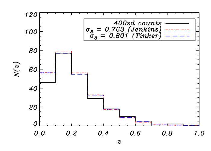
Figure 1: Observed redshift distribution (continuous black line) in the 400sd survey (Burenin et al. 2007), compared to the model predictions for $\sigma_{8}=0.763$ with the Jenkins et al. (2001) mass function (dashed blue line) and $\sigma_{8}=0.801$ with the Tinker et al. (2008) mass function (dot-dashed red line).

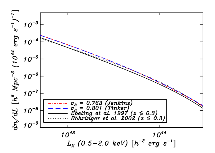
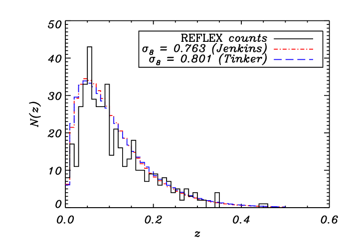
Figure 2: Consistency checks of the cluster model. Left: Local predicted XLF for the two mass functions (along with fitted $\sigma_{8}$ values), compared to observations by Ebeling et al. (1997) and Böhringer et al. (2002). Right: Same as Fig. 1, but for the REFLEX survey (Böhringer et al. 2004). One should note that the model predictions correspond to a 100% complete survey, while the actual survey is said to be at least 90% complete.

As a check of the model, we compare its predictions to other, independent observational constraints, starting with a look at the X-ray cluster counts. Using the $L_{X}-M$ relation (see Table 1) and the Jenkins et al. (2001) mass function, we fit to the 400sd survey counts (Burenin et al. 2007) to find $\sigma_{8}=0.763\pm 0.008$, keeping all other paramters fixed at their fiducial values given above. The result is shown in Figure 1. Using the Tinker et al. (2008) mass function, we obtain $\sigma_{8}=0.801\pm 0.009$. Both values agree well (within 1.5$\sigma$ in the worst case) with the WMAP-7 result of $\sigma_{8}=0.801\pm 0.030$, with $\sigma_{8}=0.773\pm 0.025$, value derived from the SPT power spectrum (Lueker et al. 2010), and lie within the range allowed by most recent measurements (Tytler et al. 2004; Cole et al. 2005; Reichardt et al. 2009; Juszkiewicz et al. 2010). Furthermore, Vikhlinin et al. (2009b) estimated the relation between $\sigma_{8}$ and $\Omega_{\rm M}$ using clusters from the 400sd survey and the RASS. They found:

$$\sigma_{8}\left(\frac{\Omega_{\rm M}}{0.25}\right)^{-0.47}=0.813\pm 0.013\,,$$ (9)

leading to $\sigma_{8}=0.795\pm 0.013$ when using $\Omega_{\rm M}=0.262$ as we did for the rest of this study, in full agreement with our estimate. This is a non-trivial and important consistency check.

The inclusion of the 15% bias in mass proves indispensable, as our best estimates for $\sigma_{8}$, when omitting this bias, drop to $\sigma_{8}=0.722\pm 0.008$ and $\sigma_{8}=0.759\pm 0.008$ for the Jenkins et al. (2001) and Tinker et al. (2008) mass functions, respectively.

To follow the remaining uncertainty associated with $\sigma_{8}$ and the mass function in the rest of this paper, all estimates will be derived using $\sigma_{8}=[0.75,0.80,0.85]$ for both mass functions.

Secondly, the predicted local X-ray Luminosity Function (hereafter XLF) is fully consistent with the measured XLF (Ebeling et al. 1997; Böhringer et al. 2002), as shown on the left-hand side of Fig. 2. This is in particular true at high luminosities, i.e., for those clusters of greatest interest to our present study.

Next, the model reproduces the redshift distribution of the REFLEX survey (Böhringer et al. 2004), a flux-limited survey (with $f_{det}=3\times 10^{-12}\,{\rm ergs/s/cm}^{2}$ in the [0.1-2.4]–keV band) covering a total area of 4.24 ster in the Southern Hemisphere. The survey contains 447 optically confirmed clusters and claims to be at least 90% complete. For an equivalent survey, our model predicts a total of 507 clusters for $\sigma_{8}=0.763$ (using the Jenkins et al. (2001) mass function), corresponding to 456 clusters when considering 90% completeness and fully consistent with the observed number. Alternatively, considering our prediction as perfect would mean that the completeness of the survey is 88.2%. On the other hand, using $\sigma_{8}=0.801$ along with the Tinker et al. (2008) mass function leads to a total of 510 clusters, hence 459 for a 90% completeness. A perfect prediction would, in this case, correspond to a completeness of 87.6%. Furthermore, as shown in Fig. 2, the overall shapes of the simulated and observed redshift distributions are in both cases in very good agreement; note, however, that the completeness is not taken into account in this plot since the redshift of the missing clusters is not known.

Finally, concerning the SZ part of our model, we have already noted that the model provides an extremely good accounting of direct SZ observations (Melin et al. 2011; Planck Collaboration et al. 2011d, c). We hence consider the model to be a reasonable empirical representation of the current data and will now apply it to study the expected X-ray properties of SZ-detected clusters. We emphasize that the model can be very easily adapted to new observational and theoretical contexts: it is built around few analytical ingredients that can be trivially changed if needed, which is an important strength of this approach.

3 SZ surveying and the Planck cluster catalog

Like the X-ray emission, the SZ effect identifies clusters through the presence of the hot, ionized intracluster medium (ICM). The SZ effect, however, is less sensitive to gas substructure, being directly proportional to the thermal energy of the ICM, and remains unaffected by cosmic dimming. As a consequence, SZ cluster surveys efficiently find clusters at high redshift.

The Planck satellite is the third generation space mission dedicated to the CMB, following COBE and WMAP. With its higher sensitivity, angular resolution and wide frequency coverage, it is the first capable of finding large numbers of galaxy clusters through the SZ effect. Its all-sky catalog of clusters detected through the SZ effect (the Planck Cluster Catalog, or PCC) will be one of the primary and novel scientific products of the mission. An early version of the catalog was recently published in Planck Collaboration et al. (2011b, ESZ) based on high signal-to-noise detections in the first tens months of data. The Planck catalogs (ESZ and Legacy catalogs) are, remarkably, the first all-sky cluster catalog since those resulting from the ROSAT All-Sky Survey (RASS) of the early 1990s (Truemper 1992). They are expected to become a workhorse for many cluster and cosmological studies.

3.1 Properties of the Expected Planck Cluster Catalog (EPCC)

We use the matched-multifilter (Herranz et al. 2002) detection algorithm described by Melin et al. (2006) to constitute the EPCC. Taking a set of sky maps at different frequencies, the algorithm simultaneously filters in both frequency and angular space to optimially extract objects with the thermal SZ spectral signature and the expected SZ angular profile. The filter is applied with a range of angular scales to produce a set of candidates at each scale, which are subsequently merged into a single catalog. Construction of the filter requires adoption of a spatial template, for which we use the modified NFW pressure profile described in Eq. (3). In essence, we assume that the filter template exactly matches the true cluster profile, which should be borne in mind as an idealized situation.

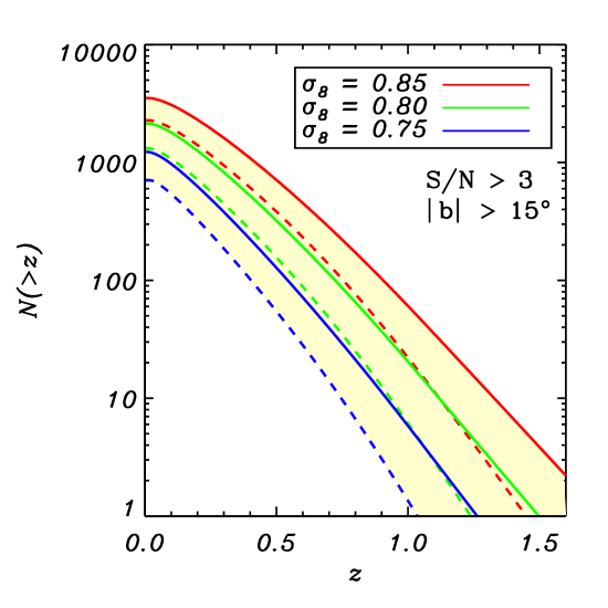
Figure 3: Predicted cumulative redshift distribution of the EPCC for a nominal mission length (14 months) and threshold $S/N>3$. The beige band illustrates modeling uncertainty due to $\sigma_{8}$ and the choice of the mass function. The solid lines are derived using the Jenkins et al. (2001) mass function while the dashed lines correspond to the Tinker et al. (2008) mass function.

We apply our filter to simulations of the Planck data set based on an early version of the Planck Sky Model (PSM). These simulations provide a set of frequency maps including primary CMB temperature anisotropies in a WMAP-5 only cosmology; Galactic synchrotron, free-free, thermal and spinning dust emission; extragalactic point sources; scan-modulated instrument noise and beams (The Planck Consortia 2005). Note, however, that we do not include any clusters in the simulations: by running our filter over these simulated maps, we seek only to quantify the total filter noise due to all instrumental and astrophysical sources.

This gives us our noise threshold at each filter scale as a function of position on the sky. With this information and our SZ scaling law, we then calculate the detectable cluster mass at a given signal-to-noise threshold as a function of redshift, over the sky and for each filter scale. By using the Jenkins et al. (2001) and Tinker et al. (2008) mass functions in our adopted cosmology, we find the EPCC distribution in mass and redshift. Figure 3 shows the resulting cumulative redshift distribution for $S/N>3$ at Galactic latitudes $|b|>15^{\circ}$ for a nominal 14-month mission, comprising two full-sky surveys, for three $\sigma_{8}$ values that illustrate the uncertainties on the determination of its value. It should be noted though, as shown above, that the cases that correspond best to the local counts are $\sigma_{8}=0.75$ for the Jenkins et al. (2001) and $\sigma_{8}=0.80$ for the Tinker et al. (2008). Our results here are consistent with the more extensive study of a dozen detection algorithms run on simulated Planck data and presented in Melin et al. (2012, in preparation).

3.2 Comparison with the RASS

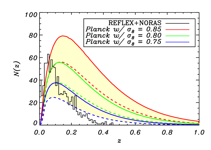
Figure 4: Comparison of the ROSAT cluster catalog (REFLEX+NORAS; black) and EPCC differential redshift distributions, shown for different values of $\sigma_{8}$. The solid lines are derived using the Jenkins et al. (2001) mass function while the dashed lines correspond to the Tinker et al. (2008) mass function. The EPCC is expected to significantly extend the depth of all-sky cluster surveys.

Since the Planck survey will be the first all-sky cluster survey since the RASS, it is of great interest to compare the EPCC to the “ROSAT Cluster Catalog”, by which we mean the sum of the REFLEX and NORAS catalogs (Böhringer et al. 2000, 2004). This is done in Fig. 4, which shows the measured ROSAT Cluster Catalog redshift distribution and the EPCC distribution for our three values of $\sigma_{8}$. From this comparison we see, as could be expected, that many clusters are common to both surveys. One of the first products of the Planck Cluster Survey will therefore be the detailed study of the relation between SZ and X-ray properties afforded by the joint catalog. Such a study will furthermore benefit from the fact that the RASS clusters are generally well-studied, allowing a number of important scaling relations to be derived. This will lead, for example, to additional tests of our empirical model and eventual modifications, all providing useful insight into cluster physics.

Moreover, prior knowledge of the X-ray-derived characteristics of these joint clusters will enable more precise recovery of their SZ properties. This is notably the case for cluster angular size, which is difficult to recover from the Planck data alone due to the size of the effecive SZ beam. This difficulty translates into noticably larger SZ flux ($Y_{SZ}$) uncertainties than if cluster size were known a priori (Melin et al. 2006) (also, Melin et al. 2010, in preparation). Clusters in the joint Planck-ROSAT catalog will therefore have significantly more precise SZ flux measurements thanks to the more precise X-ray information on cluster extent.

More surprisingly, perhaps, is the fact that some RASS clusters are not seen in the EPCC. These tend to be mostly local and extended clusters that are “resolved-out” by the Planck survey. As noted in Melin et al. (2005, 2006), the Planck selection function depends on both cluster flux and extent. The fact that the Planck selection curve cuts through the observed RASS clusters is extremely important: it will be invaluable in constraining the PCC selection function by providing well-studied clusters that fall outside of the PCC and thereby improve our understanding of the selection criteria. This is a fortunate and unusual situation that we will fully exploit when constructing the PCC.

Finally, as can be seen, we expect many new clusters not seen in the RASS. The PCC should greatly extend the redshift reach of all-sky cluster surveys over that of the RASS. The next section is dedicated to these new Planck clusters.

3.3 XMM-Newton follow-up of the new Planck clusters

Table 2: Comparison between the predicted numbers of clusters in different subsets in the EPCC for different $\sigma_{8}$ values.

Characteristics	Predicted number of clusters
	Jenkins			Tinker
	$\sigma_{8}=0.75$	$\sigma_{8}=0.80$	$\sigma_{8}=0.85$	$\sigma_{8}=0.75$	$\sigma_{8}=0.80$	$\sigma_{8}=0.85$
All	1 229	2 140	3 523	709	1 316	2 277
New clusters	425	853	1576	220	480	945
$0.8\geqslant z>1.0$	15	44	110	5	18	53
$z\geqslant 1.0$	6	20	60	1	6	21
$T\geqslant 6\rm{\ keV}$; $z\geqslant 0.5$	122	306	674	50	146	357
$T\geqslant 6\rm{\ keV}$; $0.8\geqslant z>1.0$	15	44	110	5	18	53
$T\geqslant 6\rm{\ keV}$; $z\geqslant 1.0$	6	20	60	1	6	21
$T\geqslant 6\rm{\ keV}$; $0.8\geqslant z>1.0$; $f_{x}>10^{-13}\,{\rm ergs/s/cm}^{2}$	15	44	110	5	18	53
$T\geqslant 6\rm{\ keV}$; $z\geqslant 1.0$; $f_{x}>10^{-13}\,{\rm ergs/s/cm}^{2}$	5	19	55	1	5	20

We define new Planck clusters as those with a predicted X-ray flux in the ROSAT [0.1,2.4]–keV band less than $f_{\rm X}=3\times 10^{-12}\,{\rm ergs/s/cm}^{2}$, which corresponds to the REFLEX detection limit and the deepest detection limit of the NORAS survey; we consider that all the other clusters are contained in the RASS catalogs. We then use the model to predict the X-ray properties of these new clusters in the XMM-Newton [0.5,2]–keV band. Fig. 5 shows the contours of isoflux within $[0.15-1.0]\times r_{500}$ in the XMM-Newton band over the ($z,T$) plane for these new clusters.

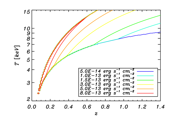
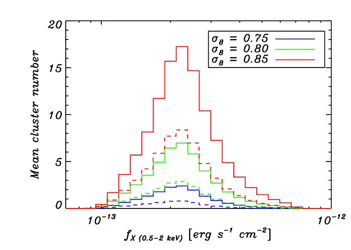
Figure 5: X-ray characteristics of new EPCC clusters within $[0.15-1.0]\times r_{500}$. Left: Contours of iso-flux in the XMM-Newton [0.5-2]–keV band plotted in the ($z,T$) plane. Right: X-ray flux distribution of new high-redshift ($z\in[0.8-1]$) clusters for $\sigma_{8}=0.75$ (blue), $\sigma_{8}=0.80$ (green) and $\sigma_{8}=0.85$ (red). The solid lines correspond to results obtained using the Jenkins et al. (2001) mass function while the dashed line was obtained using the Tinker et al. (2008) mass function.

The key point is that we expect a substantial fraction of these new clusters to be hot (or equivalently, massive) and distant; in other words, those clusters that are the most useful cosmological probes. Table 2 lists quantitative details on the distribution of these clusters. It particularly focusses on hot (i.e. with $T>6$ keV) and distant (i.e. with $z>0.5$) clusters as they fall in the most poorly filled region of the $(T,z)$ plane for known clusters. Moreover, these clusters are predicted to be very luminous, with X-ray flux in the XMM-Newton band greater than $10^{-13}\,{\rm ergs/s/cm}^{2}$ out to redshifts of order unity.

The following expression provides a useful estimate of the exposure time $t_{exp}$ (in ks) needed to measure a global temperature to $\sim 10\%$ given its X-ray flux in the XMM band:

$$t_{exp}=55\times\left(\frac{f_{x}}{10^{-13}{\rm\ ergs/s/cm}^{2}}\right)^{-1.35}\,,$$ (10)

We see that an exposure time of 55 ks is sufficient to obtain a temperature measurement for any cluster in the EPCC. Fig. 5 shows, as illustration, the histrogram of the number of new clusters with $0.8\geqslant z>1.0$ in the EPCC as a function of flux in the XMM-Newton band within $[0.15-1.0]\times r_{500}$. All of the clusters have fluxes lying in the decade below the RASS detection limit and are thus easily observable with XMM-Newton or Chandra.

In order to get an idea of the capabilities of XMM-Newton to observe such clusters based on actual measurements, we refer to the observations made of two of the four known clusters with $T\geqslant 6\rm{\ keV}$ and $0.8\geqslant z>1.0$ and consider the results obtained and required exposure times:

MS 1054-0321 (Gioia et al. 2004):

The XMM-Newton observations yield temperature, redshift (through observation of the iron line in the X-ray spectrum) and flux estimates of $T=7.2^{+0.7}_{-0.6}$ keV, $z=0.847^{+0.057}_{-0.040}$ and $f_{{\rm X\ }[0.5,2]{\rm\ keV}}=(1.9\pm 0.09)\times 10^{-13}{\rm\ ergs/s/cm}^{2}$, respectively; and they also provide a detailed image showing several components to the cluster’s structure. The effective exposure time needed was $\sim$25 ks.

RX J1226.9+3332 (Maughan et al. 2007):

The same quantities were measured in this case: $T=10.4\pm 0.6$ keV, $z=0.89$ and $f_{{\rm X\ }[0.5,2]{\rm\ keV}}=3.27\times 10^{-13}{\rm\ ergs/s/cm}^{2}$ (Vikhlinin et al. 2009a). Moreover, the observation of the temperature profile, combined with the assumption of hydrostatic equilibrium, enabled a determination of the total mass and gas mass profiles, and thus an estimate of the cluster mass: $M_{500}=5.2^{+1.0}_{-0.8}\times 10^{14}M_{\odot}$. In this case, the exposure time was $\sim$70 ks.

These clusters are good examples of the kind of objects we find in the EPCC. We conclude therefore that 25-50 ks exposures is sufficient to obtain temperature measurements to $\sim 10\%$ for any cluster in the EPCC, even out to $z\sim 1$. It is even sufficient, in some cases, to obtain mass estimates. Detailed X-ray studies of a large fraction of the new Planck clusters is hence feasible and would significantly advance our understanding of cluster structure at intermediate to high redshifts.

4 Conclusions

The Planck SZ survey will be the first all-sky cluster survey since the workhorse RASS dating from the early 1990s (Truemper 1992). The Planck Cluster Catalog (PCC) will thus satisfy the long-standing need for a deeper all-sky cluster survey. We have constructed an empirical model for cluster SZ and X-ray properties that incorporates the latest results from detailed X-ray and SZ studies. Based on this model, we expect the PCC to extend the RASS to redshifts of order unity, as shown in Figs. 3 and 4, and to contain a high fraction of hot, massive and luminous clusters. These objects are the most useful for cosmological studies, because their properties (e.g., abundance) are the most sensitive to the expansion rate and their energetics is dominated by gravity, and less affected by feedback than are less massive objects.

The expected X-ray properties of the PCC are given in Table 2. We see a significant number of new clusters, i.e., those not already contained in the RASS cluster catalogs (REFLEX and NORAS). Most should have temperatures $T>5-6$ keV and have luminosities falling in the decade just below the RASS flux limit. Interestingly, they are easy to see with current X-ray instruments, if one knows were to look. And this is our key point: these useful clusters are rare and hence can only be found by an all-sky survey, such as the Planck survey.

Our primary conclusion is that extensive X-ray follow-up of the new Planck clusters is feasible. Based on our cluster model, we estimate, for example, that XMM-Newton could measure the temperature of any newly-discovered Planck cluster to 10% with only a modest 50 ks exposure. This opens the path to important science with large follow-up programs on XMM-Newton and Chandra. A $\sim 5$ Ms program on XMM-Newton, for instance, could measure profiles and temperatures for $\sim 100$ Planck clusters at $z>0.6$, and masses for a large subset. This would be a significant increase in sample size and lead to important advances in the use of clusters as cosmological probes, as well as in our understanding of cluster physics at higher redshifts. While ambitious, this type of program is feasible and falls naturally under the category of Very Large Programmes envisaged for XMM-Newton  after 2010.

In conclusion, we expect the PCC to be unique for its ability to find rare, massive clusters out to high redshifts, and hence become a workhorse cluster catalog for many types of detailed cluster studies. In particular, we expect the PCC to initiate important X-ray follow-up programs on XMM-Newton and Chandra.