Solitary waves in the Nonlinear Dirac Equation with arbitrary nonlinearity

Abstract

We consider the nonlinear Dirac equations (NLDE’s) in 1+1 dimension with scalar-scalar self interaction $\frac{g^{2}}{k+1}({\bar{\Psi}}\Psi)^{k+1}$, as well as a vector-vector self interaction $\frac{g^{2}}{k+1}({\bar{\Psi}}\gamma_{\mu}\Psi{\bar{\Psi}}\gamma^{\mu}\Psi)^{\frac{1}{2}(k+1)}$. We find the exact analytic form for solitary waves for arbitrary $k$ and find that they are a generalization of the exact solutions for the nonlinear Schrödinger equation (NLSE) and reduce to these solutions in a well defined nonrelativistic limit. We perform the nonrelativistic reduction and find the $1/2m$ correction to the NLSE, valid when $|\omega-m|\ll 2m$, where $\omega$ is the frequency of the solitary wave in the rest frame. We discuss the stability and blowup of solitary waves assuming the modified NLSE is valid and find that they should be stable for $k<2$.

I Introduction

Beyond the usual applications in field theory, the nonlinear Dirac equation (NLDE) also emerges in various condensed matter applications. An important example being the Bose-Einstein condensate (BEC) in a honeycomb optical lattice in the long wavelength, mean field limit haddad . The multi-component BEC order parameter has an exact spinor structure and serves as the bosonic analog to the relativistic electrons in graphene.

Classical solutions of nonlinear field equations have a long history as a model of extended particles ref:extended ; soler1 . The stability of such solutions in 3+1 dimensions was studied in detail by Derrick ref:derrick . He showed that the classical solutions of the self-interacting scalar theories (with both polynomial and non-polynomial interactions) were unstable to scale transformations. However he was not able to make any conclusive statements about the spinor theories. In 1970, Soler soler1 proposed that the self-interacting 4-Fermi theory was an interesting model for extended fermions. Later, Strauss and Vasquez ref:strauss were able to study the stability of this model under dilatation and found the domain of stability for the Soler solutions. Solitary waves in the 1+1 dimensional nonlinear Dirac equation have been studied ref:Lee ; ref:Nogami in the past in case the nonlinearity parameter $k=1$, i.e. massive Gross-Neveu ref:GN (with $N=1$, i.e. just one localized fermion) and massive Thirring ref:TM models). In those studies it was found that these equations have solitary wave solutions for both scalar-scalar (S-S) and vector-vector (V-V) interactions. The interaction between solitary waves of different initial charge was studied in detail for the S-S case when $k=1$ in the work of Alvarez and Carreras ref:numerical by Lorentz boosting the static solutions and allowing them to scatter. Stability of the $k=1$ problem was also studied by Bogolubsky ref:bogol , who found using a variational method that preserved charge, that the frequencies $\omega<1/\sqrt{2}$ should be unstable. However, subsequent numerical work by Alvarez and Soler ref:soler showed that this result was incorrect (i.e. the solitary waves were numerically stable). Further analytic work on stability for the S-S model using the Shatah-Strauss formalism Shatah by Blanchard et al. Blanchard turned out to give inconclusive results in that they could not prove that the solutions to the Dirac equation were minima of the variational energy functional. Thus the domain of stability of solutions to self interacting 4-Fermi theories is still an open question.

In this paper we generalize the work of Lee, Kuo, and Gavrielides ref:Lee to arbitrary $k$ and find exact solutions for all $k$. The paper is organized as follows: In Sec. II we find rest-frame solitary wave solutions of the form $\Psi(x,t)=e^{-i\omega t}\psi(x)$, for both the case of the S-S and V-V interactions. We calculate the rest frame frequency, $\omega$, and the energy, $H$, of a solitary wave of charge $Q$, as a function of the parameters $k$ and $g$. We find the range of $k$ and $g$ values for which $\omega$ and $H$ are in the range $0<\left(\begin{array}[]{c}\omega\\ H\end{array}\right)<m$. In Sec. III we derive the nonrelativistic limit of the NLDE and find the leading term which is the nonlinear Schrödinger equation with corrections of the order of $1/2m$. Our derivation agrees with the heuristic result for $k=1$ for modification of the NLSE found earlier by ref:Toyama . We find that the correction term has the same magnitude but opposite sign for the V-V as compared to the S-S case and find that the expansion is always valid whenever $|\omega-m|\ll 2m$. In the V-V case, the NLDE solutions are numerically quite close to those of the NLSE for all values of $\omega$. However for the S-S case, when we depart from the domain of validity of the non-relativistic reduction, the solitary wave solutions depart dramatically from the NLSE limit and become double humped. We plot the crossover to this regime as a function of the nonlinearity parameter $k$. In section IV we first discuss stability of solitary waves in the NLSE using an auxiliary Lagrangian for the static solutions. We find that the criteria for stability is $0<k<2$ and that identical results are obtained using stability against scale transformations (Derrick’s theorem ref:derrick ). However the scale transformation argument leads to the conclusion that there should be unstable solitary waves in the NLDE for $k>1$ which violates continuity argument to the nonrelativistic regime. It also led to contradictions with numerical experiments at $k=1$. We then discuss the stability question in the modified NLSE (mNLSE) and show that it is essentially the same as for the NLSE. In section V we discuss how to obtain information about self-focusing in case $k=2$ and $k>2$ for both the NLSE and mNLSE assuming that the time dependent solitons are self-similar generalizations of the exact solution of the NLSE. We find that the correction terms in the mNLSE eventually dominate at late times during self-focusing and so the approximation breaks down during the late stages of self-focusing.

We conclude with a summary of our main findings as well as a discussion about the possible future directions for settling issues of stability using various approaches including numerical methods.

II Solitary wave solutions

We are interested in solitary wave solution of the NLDE given by

$$(i\gamma^{\mu}\partial_{\mu}-m)\Psi+g^{2}({\bar{\Psi}}\Psi)^{k}\Psi=0\>,$$ (1)

for the scalar-scalar interaction and

$$(i\gamma^{\mu}\partial_{\mu}-m)\Psi+g^{2}\gamma^{\mu}\Psi(\bar{\Psi}\gamma_{\mu}\Psi)(\bar{\Psi}\gamma_{\mu}\Psi{\bar{\Psi}}\gamma^{\mu}\Psi)^{\frac{1}{2}(k-1)}=0\>,$$ (2)

for the vector-vector interaction. These equations can be derived in a standard fashion from the Lagrangian

$$L=\overline{\Psi}\left(i\gamma^{\mu}\partial_{\mu}-m\right)\Psi+L_{I}\>.$$ (3)

For scalar-scalar interactions, we have

$$L_{I}=\frac{g^{2}}{k+1}(\overline{\Psi}\Psi)^{k+1}\>,$$ (4)

whereas for vector-vector interactions we have instead

$$L_{I}=\frac{g^{2}}{k+1}({\bar{\Psi}}\gamma_{\mu}\Psi{\bar{\Psi}}\gamma^{\mu}\Psi)^{\frac{1}{2}(k+1)}\>.$$ (5)

Note that in the above equations, $g^{2}$ is the dimensional coupling constant, i.e. $g^{2}=G^{2}m^{1-k}$, where $G$ is dimensionless. The $\gamma$ matrices in 2 dimensions in our convention satisfy

$$\{\gamma_{\mu},\gamma_{\nu}\}_{+}=2g_{\mu\nu};~{}~{}g_{\mu\nu}=\left(\begin{array}[]{cc}1&0\\ 0&-1\\ \end{array}\right).$$ (6)

We are looking for solitary wave solutions where the field $\Psi$ goes to zero at infinity. It is sufficient to go into the rest frame, since the theory is Lorentz invariant and the moving solution can be obtained by a Lorentz boost. In the rest frame we have that

$$\Psi(x,t)=e^{-i\omega t}\psi(x)\>.$$ (7)

We are interested in bound state solutions that correspond to positive frequency in the rest frame less than the mass parameter $m$, i.e. $0\leq\omega<m$. For these bound state solutions one requires that the energy of the solitary wave $H$ obeys $0\leq H<m$. Choosing the representation $\gamma_{0}=\sigma_{3}$, $i\gamma_{1}=\sigma_{1}$, where the $\sigma_{i}$ are the standard Pauli spin matrices, we obtain

$$i\sigma_{3}\partial_{t}\Psi+\sigma_{x}\partial_{x}\Psi-m\Psi-V_{I}\Psi=0,$$ (8)

where $V_{I}=-\frac{\partial L_{I}}{\partial{\bar{\Psi}}}$. Defining the matrix,

$$\psi(x) =\left(\begin{array}[]{c}u\\ v\end{array}\right)=R(x)\left(\begin{array}[]{c}\cos\theta\\ \sin\theta\end{array}\right)\>,$$ (13)

we obtain the following equations for $u$ and $v$. For scalar-scalar interactions, we find:

$$\frac{du}{dx}+(m+\omega)v-g^{2}(u^{2}-v^{2})^{k}v=0\>,$$

$$\frac{dv}{dx}+(m-\omega)u-g^{2}(u^{2}-v^{2})^{k}u=0\>.$$

For the vector-vector case one has instead:

$$\frac{du}{dx}+(m+\omega)v+g^{2}(u^{2}+v^{2})^{k}v=0\>,$$

$$\frac{dv}{dx}+(m-\omega)u-g^{2}(u^{2}+v^{2})^{k}u=0\>.$$

A first integral of these equations can be obtained using conservation of the energy-momentum tensor,

$$T_{\mu\nu}=i{\bar{\Psi}}\gamma_{\mu}\partial_{\nu}\Psi-g_{\mu\nu}L\>,$$

$$\partial^{\mu}T_{\mu\nu}=0\>,$$ (16)

which yields for stationary solutions

$$T_{10}=\mathrm{constant}\>,\quad T_{11}=\mathrm{constant}\>.$$ (17)

For all the cases we want to study we can write

$$T_{11}=\omega\psi^{\dagger}\psi-m{\bar{\psi}}\psi+L_{I}\>.$$ (18)

For solitary wave solutions vanishing at infinity the constant is zero and we get the useful first integral:

$$T_{11}=\omega\psi^{\dagger}\psi-m{\bar{\psi}}\psi+L_{I}=0\>.$$ (19)

Multiplying the equation of motion for either the scalar-scalar or vector-vector interaction on the left by ${\bar{\psi}}$ we have that:

$$(k+1)L_{I}=-\omega\psi^{\dagger}\psi+m{\bar{\psi}}\psi+{\bar{\psi}}i\gamma_{1}\partial_{1}\psi\>.$$ (20)

We find from Eqs. (19) and (20) that

$$\omega k\psi^{\dagger}\psi-mk{\bar{\psi}}\psi+{\bar{\psi}}i\gamma_{1}\partial_{1}\psi=0\>.$$ (21)

For the Hamiltonian density we have

$${\cal H} = T_{00}={\bar{\psi}}i\gamma_{1}\partial_{1}\psi+m{\bar{\psi}}\psi-L_{I}$$ (22)

$$\equiv h_{1}+h_{2}-h_{3}\>.$$

Each of ${h_{i}}$ are positive definite. From Eq. (19) and (20) one derives that

$$kL_{I}={\bar{\psi}}i\gamma_{1}\partial_{1}\psi\>,$$ (23)

which further implies that

$$h_{3}=\frac{1}{k}h_{1}\>.$$ (24)

In particular, for $k=1$, we obtain ${\cal H}=m{\bar{\psi}}\psi$. In terms of $(R,\theta)$ one has

$${\bar{\psi}}i\gamma_{1}\partial_{1}\psi=\psi^{\dagger}\psi\frac{d\theta}{dx}\>.$$ (25)

This leads to the simple differential equation for $\theta$ for solitary waves

$$\frac{d\theta}{dx}=-\omega_{k}+m_{k}\cos 2\theta\>,$$ (26)

where $\omega_{k}\equiv k\omega$ and $m_{k}=km$. The solution is

$$\theta(x)=\tan^{-1}(\alpha\tanh\beta_{k}x)\>,$$ (27)

where

$$\alpha=\sqrt{\frac{m_{k}-\omega_{k}}{m_{k}+\omega_{k}}}=\sqrt{\frac{m-\omega}{m+\omega}},\quad\beta_{k}=\sqrt{m_{k}^{2}-\omega_{k}^{2}}\>.$$ (28)

In what follows it is often useful to rewrite everything in terms of $\alpha$ and $\beta$. We have the relations:

$$m+\omega=\frac{\beta}{\alpha},~{}~{}m-\omega=\alpha\beta\,,~{}~{}\beta=\sqrt{m^{2}-\omega^{2}}\,.$$ (29)

II.1 Scalar-Scalar interaction

First let us look at the S-S interaction. Using Eqs. (4) and (19) we obtain

$$\omega R^{2}-mR^{2}\cos 2\theta+\frac{g^{2}}{k+1}\left(R^{2}\cos 2\theta\right)^{k+1}=0\>.$$ (30)

Thus

$$R^{2}=\left[\frac{(k+1)(m\cos 2\theta-\omega)}{g^{2}(\cos 2\theta)^{k+1}}\right]^{\frac{1}{k}}\>.$$ (31)

We have

$$\frac{d\theta}{dx}=\frac{\beta_{k}^{2}}{\omega_{k}+m_{k}\cosh 2\beta_{k}x}=-\omega_{k}+m_{k}\cos 2\theta\>,$$ (32)

so that

$$\cos 2\theta=\frac{m_{k}+\omega_{k}\cosh 2\beta_{k}x}{\omega_{k}+m_{k}\cosh 2\beta_{k}x}=\frac{m+\omega\cosh 2\beta_{k}x}{\omega+m\cosh 2\beta_{k}x}\>.$$ (33)

One important expression is

$$m\cos 2\theta-\omega=\frac{\beta_{k}^{2}}{k^{2}(\omega+m\cosh 2\beta_{k}x)}\>.$$ (34)

Using this we get

$$R^{2}=\frac{\omega+m\cosh 2\beta_{k}x}{m+\omega\cosh 2\beta_{k}x}\left[\frac{(k+1)\beta_{k}^{2}}{g^{2}k^{2}(m+\omega\cosh 2\beta_{k}x)}\right]^{\frac{1}{k}}\>,$$ (35)

Using the identities:

$$1+\alpha^{2}\tanh^{2}\beta_{k}x = \left(\frac{m\cosh 2\beta_{k}x+\omega}{m+\omega}\right){\rm sech}^{2}\beta_{k}x\>,$$

$$1-\alpha^{2}\tanh^{2}\beta_{k}x = \left(\frac{\omega\cosh 2\beta_{k}x+m}{m+\omega}\right){\rm sech}^{2}\beta_{k}x\>,$$

we obtain the alternative expression

$$R^{2}=\frac{1+\alpha^{2}\tanh^{2}\beta_{k}x}{1-\alpha^{2}\tanh^{2}\beta_{k}x}\left[\frac{(k+1)\beta_{k}^{2}{\rm sech}^{2}\beta_{k}x}{g^{2}k^{2}(m+\omega)(1-\alpha^{2}\tanh^{2}\beta_{k}x)}\right]^{\frac{1}{k}}\>.$$ (37)

The equation for $\omega$ in terms of $g^{2}$ is determined from the fact that the single solitary wave has charge Q,

$$Q=\int_{-\infty}^{\infty}dx\ \psi^{\dagger}\psi=\int_{-\infty}^{\infty}dx\ R^{2}(x)\>.$$ (38)

Thus the equation we need to solve for $\omega$ is

$$Q=\frac{1}{\beta_{k}}\left[\frac{(k+1)\beta_{k}^{2}}{g^{2}k^{2}(m+\omega)}\right]^{1/(k)}I_{k}[\alpha^{2}]\>,$$ (39)

where

$$I_{k}[\alpha^{2}]=\int^{1}_{-1}dy\,\frac{1+\alpha^{2}y^{2}}{(1-y^{2})^{\frac{1}{k}(k-1)}(1-\alpha^{2}y^{2})^{\frac{1}{k}(k+1)}}\>.$$ (40)

For $k=1$, one obtains

$$I_{1}[\alpha^{2}] = \frac{2}{1-\alpha^{2}}\>,$$ (41)

$$Q = \int_{-\infty}^{\infty}dx\ R^{2}=\frac{4\alpha}{(1-\alpha^{2})g^{2}}=\frac{2\beta}{g^{2}\omega}\>,$$

with the solution

$$\omega=\frac{m}{\sqrt{1+Q^{2}g^{4}/4}},$$ (42)

in agreement with earlier results of ref:Lee . For $k=\frac{1}{2}$, we obtain

$$I_{\frac{1}{2}}[\alpha^{2}] = \int_{-\infty}^{\infty}dy\ \frac{(1-y^{2})(1+\alpha^{2}y^{2})}{(1-\alpha^{2}y^{2})^{3}}$$

$$= \frac{4}{\alpha^{3}}\left(\tanh^{-1}\alpha-\alpha\right)$$

and

$$Q=\frac{(k+1)^{2}\beta_{k}\alpha^{2}}{k^{2}g^{4}}~{}~{}I_{\frac{1}{2}}.$$ (44)

For $k=\frac{3}{2}$, we obtain

$$I_{\frac{3}{2}}[\alpha^{2}]=-2K\left(\alpha^{2}\right)+\frac{4\omega\left(\alpha^{2}\right)}{1-\alpha^{2}}\>,$$ (45)

where $K(k)$ is the complete elliptic integral of the first kind. In general we can cast $I_{k}[\alpha^{2}]$ into the sum of two hypergeometric functions ${}_{2}F_{1}$. Letting $y=x^{\frac{1}{2}}$ we have that

$$I_{k}[\alpha^{2}]=\int_{0}^{1}dx\ \frac{x^{-\frac{1}{2}}(1+\alpha^{2}x)(1-x)^{-\frac{1}{k}(k-1)}}{(1-\alpha^{2}x)^{\frac{1}{k}(k+1)}}\>.$$ (46)

From the definition

$$\int_{0}^{1}dt\ \frac{t^{b-1}(1-t)^{c-b-1}}{(1-tz)^{a}}=\frac{\Gamma(b)\Gamma(c-b)}{\Gamma(c)}\ _{2}F_{1}(a,b,c;z)\>,$$ (47)

we find that

$$I_{k}[\alpha^{2},k]$$ (48)

$$=B\Bigl{(}\frac{1}{2},\frac{1}{k}\Bigr{)}\phantom{a}_{2}F_{1}\Bigl{(}1+\frac{1}{k},\frac{1}{2},\frac{1}{2}+\frac{1}{k};\alpha^{2}\Bigr{)}$$

$$\qquad+\alpha^{2}B\Bigl{(}\frac{3}{2},\frac{1}{k}\Bigr{)}\phantom{a}_{2}F_{1}\Bigl{(}1+\frac{1}{k},\frac{3}{2},\frac{3}{2}+\frac{1}{k};\alpha^{2}\Bigr{)}\>.$$

which, when substituted into Eq. (39) is the equation we solve to obtain $\omega$ in terms of $k$, $Q$, $m$ and $g$. Here $B(x,k)$ denotes the Beta function.

In order to see if the classical solution describes a bound state, one must calculate the value of the Hamiltonian for this solution and show that it is less than $m$. The Hamiltonian density is given by (22), so that the energy of the solitary wave is given by

$$H_{sol} = \int dx\ {\cal{H}}=\int dx\ (h_{1}+h_{2}-h_{3})$$ (49)

$$= \int dx\ \left[h_{1}\left(1-\frac{1}{k}\right)+h_{2}\right]$$

$$= H_{1}\Bigl{(}1-\frac{1}{k}\Bigr{)}+H_{2}\>,$$

where we have used Eq. (24). We find

$$H_{1} = \int dy\ R^{2}(y)\frac{d\theta(y)}{dy}$$

$$= \frac{\beta_{k}}{k(m+\omega)}\left[\frac{(k+1)\beta_{k}^{2}}{g^{2}k^{2}(m+\omega)}\right]^{\frac{1}{k}}$$

$$\times\ B\Bigl{(}\frac{1}{2},1+\frac{1}{k}\Bigr{)}\phantom{a}_{2}F_{1}\Bigl{(}1+\frac{1}{k},\frac{1}{2},\frac{3}{2}+\frac{1}{k};\alpha^{2}\Bigr{)}\>.$$

$$H_{2} = m\int dy\ R^{2}(y)\cos 2\theta(y)$$

$$= \frac{1}{\beta_{k}}\left[\frac{(k+1)\beta_{k}^{2}}{g^{2}k^{2}(m+\omega)}\right]^{\frac{1}{k}}$$

$$\times\ B\Bigl{(}\frac{1}{2},\frac{1}{k}\Bigr{)}\phantom{a}_{2}F_{1}\Bigl{(}\frac{1}{k},\frac{1}{2},\frac{1}{2}+\frac{1}{k};\alpha^{2}\Bigr{)}\>.$$

Without loss of generality, in the remaining part of this subsection we now put $m=1$ so that $0\leq\omega\leq 1$, in order to measure $\omega,H$ in units of $m$. For $k=1$ we find

$$H_{1}=\frac{2(1+\omega)}{g^{2}Q}[(1+\alpha^{2})\tanh^{-1}\alpha-\alpha]\>,$$

$$H_{2}=\frac{4}{g^{2}Q}\tanh^{-1}\alpha\>.$$ (52)

Therefore we find that the energy of the solitary wave is

$$E_{sol}=\frac{4}{g^{2}Q}\tanh^{-1}\alpha_{sol},$$ (53)

where in $\alpha_{sol}$, $\omega_{sol}=\frac{1}{\sqrt{1+Q^{2}g^{4}/4}}$. We notice that the energy of the solitary wave with $k=1$ does not depend on the width parameter $\beta$. Simplifying we obtain for $k=1$ and for all values of $g^{2}$

$$H_{sol}=\int dx\ {\bar{\psi}}\psi=\frac{2}{g^{2}Q}\sinh^{-1}(g^{2}Q/2)<1,$$ (54)

so that all the solutions are “bound states”. This agrees with the result of Lee et al. ref:Lee .

For $k=\frac{1}{2}$ one finds that

$$H_{1}= \frac{9(1-\omega)^{2}}{16g^{4}Q}[(3\alpha^{4}+2\alpha^{2}+3)\tanh^{-1}\alpha-3\alpha(1+\alpha^{2})]\>,$$

$$H_{2}= \frac{9(1+\omega)}{2g^{4}Q}[-\alpha+(1+\alpha^{2})\tanh^{-1}\alpha]\>.$$ (55)

For $Q=1$ and selected values of $k$ we determine $\omega$ and $H_{sol}$ and plot in Fig. 1 the allowed values for which $H_{sol}<1$. Note that the range of $g$ values for the existence of a bound state, as a function of $k$, is bounded from below. The functional dependence of the lower bound $g_{min}$, together with the corresponding solution $\omega(g_{min})$, as a function of $k$, are depicted in Fig. 2. We note the rapid increase of $g_{min}$ at large values of $k$. At $k\approx 2$, the upper bound of the solution $\omega(g_{min})$ becomes lower than 1, and we notice an inflection in $g_{min}(k)$. Summarizing, we find that in the S-S case, bound states exist for all values of $k$ and $g>g_{min}$.

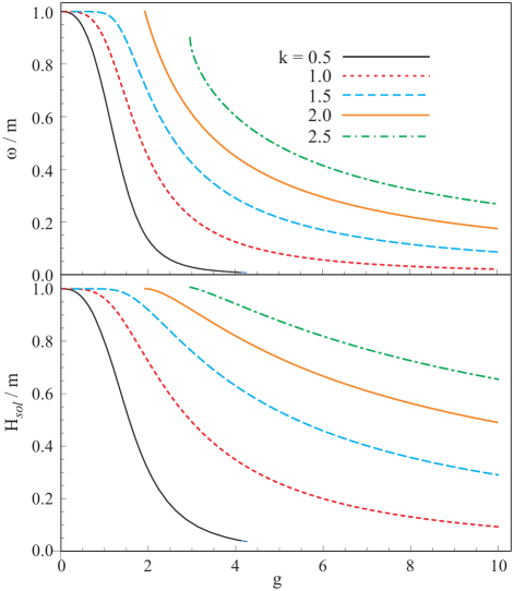
Figure 1: (Color online) NLDE bound states for the scalar-scalar interaction case: $\omega$ and $H_{sol}$ as a function of $k$ and $g$ for $Q=1$.

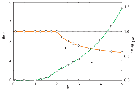
Figure 2: (Color online) Plot of the lower bound of the allowed range of $g$ values in the scalar-scale interaction case, as a function of $k$, together with the corresponding solutions, $\omega(g_{min})$. The solid lines are intended only as a guide to the eye.

II.2 Vector-Vector interaction

For the V-V interaction case, we obtain

$$L_{I}=\frac{g^{2}}{k+1}({\bar{\Psi}}\gamma_{\mu}\Psi{\bar{\Psi}}\gamma^{\mu}\Psi)^{\frac{1}{2}(k+1)}=\frac{g^{2}}{k+1}R^{2(k+1)}\>.$$ (56)

Eq. (19) now becomes

$$\omega R^{2}-mR^{2}\cos 2\theta+\frac{g^{2}}{k+1}R^{2(k+1)}=0\>.$$ (57)

Thus

$$R^{2}=\left[\frac{(k+1)(m\cos 2\theta-\omega)}{g^{2}}\right]^{\frac{1}{k}}\>.$$ (58)

This can be rewritten in the following two forms:

$$R^{2}=\left[\frac{(k+1)\beta_{k}^{2}}{g^{2}k^{2}(\omega+m\cosh 2\beta_{k}x)}\right]^{\frac{1}{k}}$$

$$=\left[\frac{(k+1)\beta_{k}^{2}{\rm sech}^{2}\beta_{k}x}{g^{2}k^{2}(m+\omega)(1+\alpha^{2}\tanh^{2}\beta_{k}x)}\right]^{\frac{1}{k}}\>.$$ (59)

The equation for $\omega$ can then be determined by using the charge defined in Eq. (38). This gives

$$Q=\frac{1}{\beta_{k}}\left[\frac{(k+1)\beta_{k}^{2}}{g^{2}k^{2}(m+\omega)}\right]^{1/(k)}\hat{I}_{k}[\alpha^{2}]\>,$$ (60)

where

$$\hat{I}_{k}[\alpha^{2}]=B\Bigl{(}\frac{1}{2},\frac{1}{k}\Bigr{)}\phantom{a}_{2}F_{1}\Bigl{(}\frac{1}{2},\frac{1}{k},\frac{1}{2}+\frac{1}{k};-\alpha^{2}\Bigr{)}\>.$$ (61)

For $k=1$, this gives

$$Q=\int_{-\infty}^{\infty}dx\ R^{2}=\frac{4\tan^{-1}\alpha}{g^{2}}\>,\quad\omega=m\cos(g^{2}Q/2)\>.$$ (62)

This imposes the restriction on the coupling constant, i.e. $g^{2}Q<\pi$ so that the spectrum is composed of positive-energy fermion states. On the other hand, for $k=\frac{1}{2}$ this gives

$$Q=\frac{9(1+\omega)}{2g^{4}}[\alpha-(1-\alpha^{2})\tan\alpha]\>.$$ (63)

The energy of the solitary wave is given by integrating the Hamiltonian density (22), and we obtain

$$H_{sol} = \int dx\ {\cal{H}}=\int dx\ (h_{1}+h_{2}-h_{3})$$ (64)

$$= H_{1}\Bigl{(}1-\frac{1}{k}\Bigr{)}+H_{2}\>,$$

where

$$H_{1} = \frac{\beta_{k}}{k(m+\omega)}\left[\frac{(k+1)\beta_{k}^{2}}{g^{2}k^{2}(m+\omega)}\right]^{\frac{1}{k}}$$

$$\times\ B\Bigl{(}\frac{1}{2},1+\frac{1}{k}\Bigr{)}\phantom{a}_{2}F_{1}\left(1+\frac{1}{k},\frac{1}{2},\frac{3}{2}+\frac{1}{k};-\alpha^{2}\right)\>,$$

$$H_{2} = \frac{1}{\beta_{k}}\left[\frac{(k+1)\beta_{k}^{2}}{g^{2}k^{2}(m+\omega)}\right]^{\frac{1}{k}}$$

$$\times\ B\Bigl{(}\frac{1}{2},\frac{1}{k}\Bigr{)}\Bigl{[}2\ _{2}F_{1}\left(\frac{1}{k},\frac{1}{2},\frac{1}{2}+\frac{1}{k};-\alpha^{2}\right)$$

$$\qquad\qquad\qquad-\phantom{a}_{2}F_{1}\Bigl{(}\frac{1}{2},\frac{1}{k},\frac{1}{k}+\frac{1}{2};-\alpha^{2}\Bigr{)}\Bigr{]}\>.$$

Without any loss of generality, in the remaining part of this subsection we put $Q=m=1$, i.e. we measure $\omega,H$ in units of $m$ so that $0\leq\omega\leq 1$. For $k=1$, we find

$$H_{1} = \frac{2(1+\omega)}{g^{2}}[\alpha-(1-\alpha^{2})\tan^{-1}\alpha]\>,$$ (67)

$$H_{2} = \frac{4\alpha}{g^{2}(1+\alpha^{2})}\>.$$

For $k=1$, we have an analytic solution:

$$H_{sol}=\int dx\ {\bar{\psi}}\psi=\frac{2}{g^{2}}\sin(g^{2}/2)<1\>,$$ (68)

since $0<g^{2}<\pi$, thereby showing the bound-state behaviour even in the vector case. For $k=\frac{1}{2}$, one finds

$$H_{1}= \frac{9(1+\omega)^{2}}{16g^{4}}[(3\alpha^{4}-2\alpha^{2}+3)\tan^{-1}\alpha-3\alpha(1-\alpha^{2})]\>,$$

$$H_{2}= \frac{9(1+\omega)}{4g^{4}}[(1+\alpha^{2})\tan^{-1}\alpha-\frac{\alpha(1-\alpha^{2})}{(1+\alpha^{2})}]\>,$$

$$H_{3}= 2H_{1}\>.$$ (69)

In Fig. 3 we map out the allowed values of $\omega$ and $g^{2}$ for various values of $k$. The allowed range of $g$ values for the existence of a bound state, as a function of $k$, has both a lower and an upper bound, and the domain shrinks as $k$ increases. Around $k$=2.5, these bounds cross, and no bound states are possible for $k>2.5$. The functional dependence of $g_{min}$ and $g_{max}$, together with the corresponding solutions $\omega(g_{min})$ and $\omega(g_{max})$, as a function of $k$, are depicted in Fig. 4. As in the S-S case, $\omega(g_{min})$ becomes less than 1 for $k\approx 2$, and we notice an inflection in $g_{min}(k)$. However, we now find that $\omega(g_{max})$ approaches one in case $k>2$.

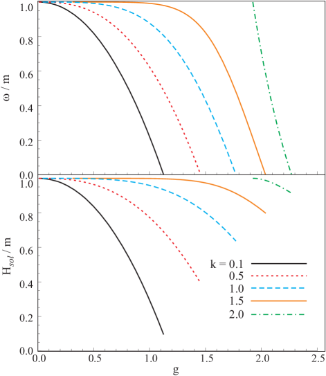
Figure 3: (Color online) NLDE bound states for the vector-vector interaction case: $\omega$ and $H_{sol}$ as a function of $k$ and $g$.

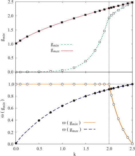
Figure 4: (Color online) Plot of the lower and upper bounds of the allowed range of $g$ values in the vector-vector interaction case, as a function of $k$ (top panel). In the lower panel we depict the $k$ dependence of the corresponding solutions $\omega(g_{min})$ and $\omega(g_{max})$, respectively. The solid lines are intended only as a guide to the eye.

III Connection to the solutions of the NLSE

In this section we will perform the nonrelativistic reduction of the NLDE to determine how it compares to the NLSE. The NLDE can be written as

$$i\sigma_{3}\partial_{t}\Psi+\sigma_{x}\partial_{x}\Psi-m\Psi-V_{I}\Psi=0\>.,$$ (70)

where $V_{I}=-\frac{\partial L_{I}}{\partial{\bar{\Psi}}}=-g^{2}({\bar{\psi}}\psi)^{k}$. Next, we use Moore’s decoupling method ref:Moore and write

$$V_{I}[\lambda]=\frac{1+\sigma_{3}}{2}V_{I}+\lambda\frac{1-\sigma_{3}}{2}V_{I}\>.$$ (71)

We see that $V_{I}[\lambda=1]=V_{I}$. It has been shown that doing a perturbation theory in $\lambda$ is a valid way of obtaining the corrections to the nonrelativistic theory. Moore’s decoupling technique was used for the (relativistic) hydrogen atom using conventional Rayleigh-Schrödinger perturbation theory and computer algebra and it was shown that the perturbative solution converges to the correct solution ref:Moore . It has been applied successfully to the relativistic calculations on alkali atoms and represents one of the many relativistic perturbative schemes investigated by Kutzelnigg ref:Kutz . We will show that this procedure leads to the heuristically derived nonrelativistic reduction of the NLDE as discussed by Toyama et al. for the case $k=1$ ref:Toyama .

We let

$$\Psi_{0}(x) =e^{-i\omega t}\left(\begin{array}[]{c}u_{0}\\ v_{0}\end{array}\right)\>,$$ (74)

be a solution of the theory when $\lambda=0$. For scalar-scalar interactions, we find:

$$\frac{du_{0}}{dx}+(m+\omega)v_{0}=0\>,$$

$$\frac{dv_{0}}{dx}+(m-\omega)u_{0}-g^{2}(u_{0}^{\star}u_{0}-v_{0}^{\star}v_{0})^{k}u_{0}=0\>.$$

From Eq. (III) we obtain

$$\frac{du_{0}}{dx}=-(m+\omega)v_{0}\>.$$ (76)

This leads to the following equation for $u_{0}$:

$$-\frac{(u_{0})_{xx}}{2m}+(V_{I}-\epsilon_{0})\left(1+\frac{\epsilon_{0}}{2m}\right)u_{0}=0\>,$$ (77)

where $\epsilon_{0}=\omega-m$. We notice that the expansion parameter is $\epsilon_{0}/(2m)$. When $|\omega-m|/(2m)\ll 1$ is satisfied then we can be sure that the NLDE solutions go over to the NLSE solutions. However we will find that in the V-V case, the reduction numerically appears valid over a wider range. The relevant Schrödinger-like equation is:

$$-\frac{(u_{0})_{xx}}{2m}+\hat{V}_{I}u_{0}={\hat{E}}u_{0}\>,$$ (78)

where

$$\hat{V}_{I}=V_{I}\Bigl{(}1+\frac{\epsilon_{0}}{2m}\Bigr{)}\>,\qquad{\hat{E}}=\epsilon_{0}(1+\frac{\epsilon_{0}}{2m})\>.$$ (79)

For consistency we need to expand $V_{I}$ to first order in $1/2m$. For the scalar scalar case, we have

$$V_{I} =-g^{2}(u_{0}^{\star}u_{0}-v_{0}^{\star}v_{0})^{k}$$

$$\rightarrow-g^{2}\left[(u_{0}^{\star}u_{0})^{k}-\frac{k}{4m^{2}}(u_{0}^{\star}u_{0})^{k-1}(u_{0})_{x}^{\star}(u_{0})_{x}\right].$$

The resulting modified nonlinear Schrödinger equation (mNLSE) can be derived from the Lagrangian:

$$L= i\psi^{\star}\partial_{t}\psi-\frac{1}{2m}\left[\psi^{\star}_{x}\psi_{x}\left(1+\frac{{\hat{g}}^{2}}{2m}(\psi^{\star}\psi)^{k}\right)\right]$$ (81)

$$+\frac{{\hat{g}}^{2}}{k+1}(\psi^{\star}\psi)^{k+1},$$

and the Hamiltonian is given by

$$H=\!\!\int\frac{dx}{2m}\left[\psi^{\star}_{x}\psi_{x}\left(1+\frac{{\hat{g}}^{2}}{2m}(\psi^{\star}\psi)^{k}\right)\right]-\frac{{\hat{g}}^{2}}{k+1}(\psi^{\star}\psi)^{k+1}\>,$$ (82)

where ${\hat{g}}^{2}=g^{2}[1+\epsilon_{0}/(2m)]$.

In the case of the V-V interaction, the nonrelativistic reduction of the NLDE is similar to the previous case with the difference that

$$V_{I}^{v-v} =-g^{2}(u_{0}^{\star}u_{0}+v_{0}^{\star}v_{0})^{k}$$

$$\rightarrow-g^{2}\left[(u_{0}^{\star}u_{0})^{k}+\frac{k}{4m^{2}}(u_{0}^{\star}u_{0})^{k-1}(u_{0})_{x}^{\star}(u_{0})_{x}\right].$$

The resulting modified nonlinear Schrödinger equation (mNLSE) can be derived from the Lagrangian:

$$L= i\psi^{\star}\partial_{t}\psi-\frac{1}{2m}\left[\psi^{\star}_{x}\psi_{x}\left(1-\frac{{\hat{g}}^{2}}{2m}(\psi^{\star}\psi)^{k}\right)\right]$$ (84)

$$+\frac{{\hat{g}}^{2}}{k+1}(\psi^{\star}\psi)^{k+1},$$

and the Hamiltonian is given by

$$H=\!\!\int\frac{dx}{2m}\left[\psi^{\star}_{x}\psi_{x}\left(1-\frac{{\hat{g}}^{2}}{2m}(\psi^{\star}\psi)^{k}\right)\right]-\frac{{\hat{g}}^{2}}{k+1}(\psi^{\star}\psi)^{k+1},$$ (85)

where ${\hat{g}}^{2}=g^{2}[1+\epsilon_{0}/(2m)]$.

Thus we see that the resulting theory in the large $1/2m$ limit (as well as when $|\omega-m|\ll 2m$), in both S-S and V-V cases reduces to the modified NLSE equation. The first correction has the same magnitude but opposite sign for the two cases.

III.1 Comparison with the exact solution of the NLSE and mNLSE

Here we want to compare the NLDE with the exact solution of the of the NLSE as well as mNLSE for arbitrary $k$. We will give numerical comparison both when the criterion $|\omega-m|\ll 2m$ is satisfied and for general $\omega$. We will find that the V-V NLDE case has solutions that track those of the NLSE for a broader range of $\omega$.

First let us obtain solutions to the NLSE for arbitrary $k$. The NLSE is defined by the Lagrangian

$$L={\frac{i}{2}}\int dx\ (\mbox{$\psi^{\ast}$}\psi_{t}-\mbox{$\psi^{\ast}$}_{t}\psi)-H\>,$$ (86)

where for the S-S interaction

$$H=\int dx\ \left[\frac{1}{2m}\nabla\mbox{$\psi^{\ast}$}\nabla\psi-g^{2}{\frac{(\mbox{$\psi^{\ast}$}\psi)^{k+1}}{k+1}}\right]\>.$$ (87)

This leads to the equation of motion

$$i\,{\frac{\partial\psi}{\partial t}}+\frac{1}{2m}\left(\frac{\partial\psi}{\partial x}\right)^{2}+g^{2}(\mbox{$\psi^{\ast}$}\psi)^{k}\psi=0\>.$$ (88)

If we make the ansatz

$$\psi(x,t)=r(y)\exp[i(mvy-\omega t+\delta)]\,,~{}~{}y=x-vt\,,$$ (89)

then it is easy to show that $r(y)$ satisfies the equation

$$r^{\prime\prime}(y)-\Omega r(y)+g^{2}r^{2k+1}(y)=0\,,$$ (90)

where $\Omega=-(\omega+\frac{mv^{2}}{2})$. Equation (90) has an exact solution

$$r(y)=A{\rm sech}^{1/k}[D(y+y_{0})]\,,$$ (91)

provided

$$\Omega=\frac{D^{2}}{2mk^{2}}\>,\quad A^{2k}=\frac{(k+1)D^{2}}{2mg^{2}k^{2}}\,.$$ (92)

The mass density in the rest frame ($v=0$) is given by

$$\rho=\mbox{$\psi^{\ast}$}\psi=\left[\frac{(k+1)D^{2}}{2mg^{2}k^{2}}\right]^{1/k}{\rm sech}^{2/k}[D(x+x_{0})]\>.$$ (93)

Let us now obtain the solutions of the mNLSE. We first notice that to the first order in $1/2m$, the static mNLSE equation in both S-S and V-V cases is given by

$$-(u_{0})_{xx}+(m^{2}-\omega^{2})u_{0}-(m+\omega)g^{2}[u_{0}^{\star}u_{0}]^{k}u_{0}=0\,,$$ (94)

which has the exact solution

$$u_{0}(x)=A{\rm sech}^{1/k}[\beta_{k}(x+x_{0})]\,,$$ (95)

with

$$A^{2k}=\frac{(k+1)\beta_{k}^{2}}{(m+\omega)g^{2}k^{2}}\,.$$ (96)

Hence for mNLSE, the mass density in the rest frame ($v=0$) is given by

$$\rho=\mbox{$\psi^{\ast}$}\psi=\left[\frac{(k+1)\beta_{k}^{2}}{(m+\omega)g^{2}k^{2}}\right]^{1/k}{\rm sech}^{2/k}[\beta_{k}(x+x_{0})]\>.$$ (97)

We will now compare the NLSE and mNLSE solutions with the solutions of the NLDE. In making these comparisons we will in all cases compare the solutions for the charge density (which is the mass density for the NLSE and mNLSE).

III.2 Scalar-Scalar interaction

One can rewrite the charge density $\rho=R^{2}$, Eq.  (37) in the following form which isolates the previous solution to the NLSE.

$$\rho=\left[\frac{\beta_{k}^{2}(k+1)}{g^{2}k^{2}(m+\omega)}\right]^{1/k}{\rm sech}^{2/k}\beta_{k}x~{}~{}f(\alpha,\beta,x),$$

$$f(\alpha,\beta,x)=\frac{1+\alpha^{2}\tanh^{2}\beta_{k}x}{(1-\alpha^{2}\tanh^{2}\beta_{k}x)^{(1+1/k)}}\>.$$ (98)

If we compare NLSE and S-S case, we find that $\rho(x=0)$ is same in both cases only if we can identify $D$ with $\beta_{k}$. We also have that $f(\alpha,\beta,x=0)=1$, so that with this identification, the charge and mass densities have the same value as a function of $k$ for the NLSE and NLDE.

On the other hand, $\rho(x=0)$ is strictly identical for S-S and mNLSE cases and no identification needs to be made.

We have seen that the nonrelativistic limit is obtained when $|\omega-m|/2m\ll 1$. In Fig. 5, we compare the solutions to the NLSE and NLDE when $\omega/m=0.9$ (top panel) and $\omega/m=0.3$ (bottom panel), for $k=1$. In the latter case, we notice that the solution to the NLDE is double humped. For any $\omega\leq\omega_{c}(k)$ for which the solution becomes double humped in the NLDE is shown in Fig. 6.

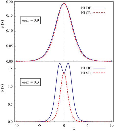
Figure 5: (Color online) Comparison of the NLSE and NLDE solutions in the case of scalar-scalar interactions for $k=1$, and $\omega/m=0.9$ (top panel) and $\omega/m=0.3$ (bottom panel), respectively.

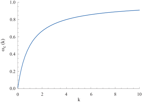
Figure 6: (Color online) Critical value, $\omega_{c}(k)$, for any $\omega\leq\omega_{c}(k)$ the solution of the NLDE equation becomes double humped in the case of scalar-scalar interactions.

III.3 Vector-Vector interaction

Now we rewrite the solution found for the charge density $\rho=R^{2}$, Eq. (59) in the following form:

$$\rho=\left[\frac{\beta_{k}^{2}(k+1)}{g^{2}k^{2}(m+\omega)}\right]^{1/k}{\rm sech}^{2/k}\beta_{k}x~{}~{}f(\alpha,\beta,x)\>,$$

$$f(\alpha,\beta,x)=\ {(1+\alpha^{2}\tanh^{2}\beta_{k}x)^{-1/k}}\>.$$ (99)

We have seen that the nonrelativistic limit is obtained when $|\omega-m|/2m\ll 1$. For the V-V case, the modification of the NLSE result is small even at very small $\omega/m$ and, unlike in the case of S-S interactions, the NLDE solution never becomes double humped. In Fig. 7 we compare the solutions of the NLSE and NLDE when $\omega/m=0.01$ and $k=1$. The main difference compared to the S-S case is that the convergence to the nonrelativistic limit as $\omega/m\rightarrow 1$, occurs from above in the vector case instead of from below as in the scalar case (see Fig. 7 and the top panel of Fig. 5). Again notice that $\rho(x=0)$ is identical in NLSE and V-V case only if we identify $D$ with $\beta_{k}$.

On the other hand, $\rho(x=0)$ is strictly identical for mNLSE and V-V case and no identification needs to be made.

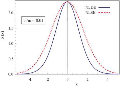
Figure 7: (Color online) Comparison of the NLSE and NLDE solutions in the case of vector-vector interactions for $k=1$ and $\omega/m=0.01$.

IV stability of static solutions

The stability of the solitary waves of the NLSE have been studied for a long time. A recent discussion of this is found in review . In this section we will first show that an analysis of the solutions of the NLSE equation using the slope criterion ($\frac{dM(\omega)}{d\omega}<0$ for stability) where $M$ is the mass of the Solitary wave and $\omega$ the frequency gives the same result ($0<k<2$) as an analysis based on whether a scale transformations raises or lowers the energy of the solitary wave. The latter criterion is similar to the arguments first used by Derrick ref:derrick in his study of the relativistic scalar field theories. We will then use a similar scaling argument first made by Bogolubsky ref:bogol for the NLDE equation to obtain a criterion for stability. We will find that the results of this approach do not agree with a smooth continuation of the result for the NLSE. We will discuss the most likely reason for the failure of this method when applied to the NLDE. Finally we will look at the stability in the mNLSE which contains the first relativistic correction to the NLSE and show that it gives essentially the same criterion as that found for the NLSE, i.e. when $0<k<2$ we expect the solutions to be stable.

Most studies of the stability of static solutions of the NLSE rely on the existence of a variational principle

$$\delta{\mathcal{E}}=\delta(H-\omega M)=0\>,$$ (100)

from which the ordinary differential equation for the solution $u(x,\omega)$ can be derived. Here the NLSE Hamiltonian is

$$H=\int dx\ \left[\frac{1}{2m}\partial_{x}\psi^{\star}\partial_{x}\psi-\frac{g}{k+1}(\psi^{\star}\psi)^{k+1}\right]\>,$$ (101)

and the mass is given by

$$M=\int dx\psi^{\star}\psi\>.$$ (102)

This variational principle is quite similar to the one used to study the stability in the generalized KdV systems K ; DK ; VK ; cooper3 . There one derives the solitary wave equation from

$$\delta\epsilon=\delta(H-cP)=0\,,$$ (103)

where $c$ is the velocity of the solitary wave while the generalized KdV equation is

$$u_{t}+u^{l-2}u_{x}$$

$$+\alpha[2u^{p}u_{xxx}+4pu^{p-1}u_{x}u_{xx}+p(p-1)u^{p-2}(u_{x})^{3}]=0\,.$$

This can be derived from the Hamiltonian

$$H=\int dx\left[-\frac{u^{l}}{l(l-1)}-\alpha u^{p}(u_{x})^{2}\right]\,,$$ (105)

and the corresponding momentum P is given by

$$P=\int dx\frac{1}{2}u^{2}(x,t)\,.$$ (106)

Stable solitary waves of the form $\psi(x,t)=u(x,\omega)e^{-i\omega t}$ need to be local energy minimizers of the functional (100). Based on linearized perturbation theory and using this variational principle Vakhitov and Kolokolov VK showed that a necessary criterion for stability is that

$$\frac{dM(\omega)}{d\omega}<0.$$ (107)

This criteria is the analogue of the result found for the generalized KdV equations by Karpman K and Dey and Khare DK who obtained that stable solitary waves for that system of equations required

$$\frac{dP(c)}{dc}>0.$$ (108)

The exact solution for $u(x)$ of NLSE for arbitrary $k$ is given in (91). Using that solution, one finds that the mass has the following dependence on $\omega$:

$$M=C(-\omega)^{(2-k)/(2k)}\>,$$ (109)

and the necessary criterion for stability is

$$k<2.\>$$ (110)

Another approach to stability, which leads to the same result as (110), is based on whether a scale transformation which keeps the mass $M$ invariant, raises or lowers the energy of a solitary wave. For the NLSE with Hamiltonian

$$H = \int dx\ \left[\partial_{x}\psi^{\star}\partial_{x}\psi-\frac{g}{k+1}(\psi^{\star}\psi)^{k+1}\right]$$ (111)

$$\equiv H_{1}-H_{2}\>,$$

both $H_{1}$ and $H_{2}$ are positive definite. A static solitary wave solution can be written as

$$\psi(x,t)=r(x)e^{-i\omega t}\>.$$ (112)

The exact solution has the property that it minimizes the Hamiltonian subject to the constraint of fixed mass as a function of a stretching factor $\beta$. This can be seen by studying a variational approach as done in cooper3 or by directly studying the effect of a scale transformation that respects conservation of mass.

In the latter approach, which generalizes the method used by Derrick ref:derrick , we let

$$x\rightarrow\beta x\>,$$ (113)

and consider

$$\psi_{\beta}(x)=\beta^{\frac{1}{2}}r(\beta x)e^{-i\omega t}\>,$$ (114)

this leaves

$$M=\int dx\ \psi^{\star}\psi=\int dx\ \psi_{\beta}^{\star}\psi_{\beta}\>,$$ (115)

unchanged. One defines $H_{\beta}$ as the value of $H$ for the stretched solution $\psi_{\beta}$. One then finds that

$$\frac{\partial H_{\beta}}{\partial\beta}\Bigr{|}_{\beta=1}=0\>,$$ (116)

is consistent with the equations of motion, and the stable solutions satisfy

$$\frac{\partial^{2}H_{\beta}}{\partial\beta^{2}}\geq 0\>.$$ (117)

If we write $H$ in terms of the two positive definite pieces $H_{1}$, $H_{2}$, then

$$H_{\beta}=\beta^{2}H_{1}-\beta^{k}H_{2}\>.$$ (118)

We find:

$$\frac{\partial H_{\beta}}{\partial\beta}=2\beta H_{1}-(k)\beta^{k-1}H_{2}\>.$$ (119)

We obtain

$$\frac{\partial H_{\beta}}{\partial\beta}|_{\beta=1}=0\rightarrow H_{1}=\frac{k}{2}H_{2}\>.$$ (120)

This result is consistent with the equation of motion. The second derivative is given by

$$\frac{\partial^{2}H_{\beta}}{\partial\beta^{2}}=2H_{1}-k(k-1)\beta^{k-2}H_{2}\>,$$ (121)

which when evaluated at the stationary point yields

$$\frac{\partial^{2}H_{\beta}}{\partial\beta^{2}}=2(2-k)H_{1}\>.$$ (122)

This result indicates that solutions are unstable to changes in the width (compatible with the conserved mass) when $k>2$. The case $k=2$ is the marginal case where it is known that blowup occurs at a critical mass (see for example Ref. cooper3, ). The result found above for the NLSE has also been found by various other methods such as linear stability analysis and using strict inequalities. Numerical simulations have been done for the critical case $k=2$ showing that blowup (self-focusing) occurs when the mass $M>2.72$ numerical . For $k>2$ a variety of analytic and numerical methods have been used to study the nature of the blowup at finite time kevrekedis .

Let us now apply this scaling argument, as was done by Bogolubsky ref:bogol ), to the 1+1 dimensional NLDE. Again we will assume that the exact solution minimizes $H_{\beta}$ when $\beta=1$ with the constraint that the charge is kept fixed. (The validity of this assumption will be challenged below. All that is known is that $H_{\beta}$ is a stationary point at the solution.)

Our exact solution is of the form

$$\psi(x)=\left(\begin{array}[]{c}u\\ v\end{array}\right)=R(x)\left(\begin{array}[]{c}\cos\theta\\ \sin\theta\end{array}\right)e^{-i\omega t}\>.$$ (123)

Because we want to keep the charge fixed, we consider the following stretched solution:

$$\psi_{\beta}(x)=\left(\begin{array}[]{c}u\\ v\end{array}\right)=\beta^{\frac{1}{2}}R(\beta x)\left(\begin{array}[]{c}\cos\theta(\beta x)\\ \sin\theta(\beta x)\end{array}\right)e^{-i\omega t}\>.$$ (124)

The value of the Hamiltonian

$$H = \int dx\ \Bigl{[}{\bar{\psi}}i\gamma_{1}\partial_{1}\psi+m{\bar{\psi}}\psi-\frac{g^{2}}{k+1}({\bar{\psi}}\psi)^{k+1}\Bigr{]}$$ (125)

$$\equiv H_{1}+H_{2}-H_{3}\>,$$

for the stretched solution is

$$H_{\beta}=\beta H_{1}+H_{2}-\beta^{k}H_{3}\>,$$ (126)

where again $H_{i}$ are all positive definite. The first derivative is

$$\frac{\partial H_{\beta}}{\partial\beta}=H_{1}-k\beta^{k-1}H_{3}\>.$$ (127)

At the minimum, setting $\beta=1$, we find in general

$$H_{3}=\frac{1}{k}H_{1}\>,$$ (128)

which is consistent with the equation of motion result we obtained earlier, see Eq.  (24). We see that for $k=1$ the energy is given by just $H_{2}$. The second derivative yields:

$$\frac{\partial^{2}H_{\beta}}{\partial\beta^{2}}=-k(k-1)\beta^{k-2}H_{3}\>.$$ (129)

From this we see that if $k>1$, this analysis (if correct) would suggest that solitary waves are unstable to small changes in the width. For $0<k<1$ the solitary waves are stable to this type of perturbation. This argument does not depend on $L_{I}$ as long as $L_{I}$ is positive definite. The same result is valid for both scalar and vector type interactions.

For $k=1$, this argument does not give any insight into whether the solutions are stable. However, it is known that the solitary waves discussed here for $k=1$, do appear to be stable numerically. Further, when they are scattered in numerical experiments, they interchange charge and energy, and sometimes show bound state production. Detailed numerical simulations have been performed by Alvarez and Carreras ref:numerical . These results contradict the work of Bogolubsky ref:bogol who studied changes in the frequency $\omega$ while keeping the charge fixed. There a similar analysis gave a maximum for the Hamiltonian when $\omega<1/\sqrt{2}$, even though, as remarked above, numerical studies show that solitary waves in that frequency range are in fact stable.

We have already shown above that the solutions of the NLDE reduce to those of the NLSE in the nonrelativistic limit. Assuming continuity arguments apply, one would expect that there would be at least a range of values of $\omega$ for which the solutions to the NLDE are stable for $k<2$.

So one needs to understand the reason for this apparent discrepancy. The main reason for assuming instability when the second derivative of $H(\beta)$ is positive, is that the stable solutions to the Dirac equation are at least relative minima of the effective action. However, the study by Blanchard et al. Blanchard to find an analytic criterion for stability in the 1+1 dimensional NLDE using the Shatah-Strauss formalism found that bound states were not local minima on the manifold of constant charge. This result is quite different from what happens in the NLSE where the bound states are local minima on the manifold of constant mass. So one cannot assume that the sign found in Eq. (129) yields information about the stability of the solution. On the other hand we can assume by continuity that there is a region where the analysis of stability in the mNLSE will give us information about stability at least in the regime where the expansion parameter $\epsilon/2m$ is small. For the mNLSE we can use the scaling argument or the auxiliary variational approach to discuss stability. It is interesting that Derrick ref:derrick in his seminal paper was unable to find a suitable method for discussing stability for self-interacting spinor theories.

For the mNLSE the Hamiltonian for the S-S interactions is given by

$$H=\int\frac{dx}{2m}\left[\psi^{\star}_{x}\psi_{x}\left(1+\frac{g^{2}}{2m}(\psi^{\star}\psi)^{k}\right)\right]-\frac{g^{2}}{k+1}(\psi^{\star}\psi)^{k+1}.$$ (130)

It is well known that using stability with respect to scale transformation to understand domains of stability applies to this type of Hamiltonian. This Hamiltonian is a sum of two positive and one negative term i.e.

$$H=H_{1}+H_{2}-H_{3}\>.$$ (131)

For the V-V case, the Hamiltonian is instead

$$H=H_{1}-H_{2}-H_{3}\>.$$ (132)

We also know that $H_{2}$ is of order $g^{2}/2m$ and is presumed small. If we again make a scale transformation on the solution which preserves the mass $M=\int\psi^{\star}\psi dx$,

$$\psi_{\beta}=\beta^{1/2}\psi(\beta x)\>,$$ (133)

we obtain

$$H=\beta^{2}H_{1}\pm\beta^{2+k}H_{2}-\beta^{k}H_{3}\>.$$ (134)

Here the upper(lower) sign corresponds to the S-S (V-V) case. The first derivative is:

$$\frac{\partial H}{\partial\beta}=2\beta H_{1}\pm(2+k)\beta^{k+1}H_{2}-k\beta^{k-1}H_{3}\>.$$ (135)

Setting the derivative to zero at $\beta=1$ gives the equation consistent with the equations of motion:

$$kH_{3}=2H_{1}\pm(2+k)H_{2}\>.$$ (136)

The second derivative at $\beta=1$ can now be written as

$$\frac{\partial^{2}H}{\partial\beta^{2}}=(4-2k)H_{1}\pm 2(2+k)H_{2}\>.$$ (137)

This will be positive for $k<2$ and the addition of a small $H_{2}$ should extend the stability of the solutions beyond $k=2$ in the S-S case. However, in the V-V case there is a somewhat lower region of stability. At $k=2$, as we shall see below, the usual NLSE solitary waves blow up once the mass exceeds a critical value. For $k=1$, numerical experiments for the time evolution of an initial wave of the form

$$\psi(x,t=0)=\sqrt{\beta/2}{\rm sech}(\beta y)e^{i(mvx-\frac{1}{2}mv^{2}t-\epsilon_{0}t)}$$ (138)

at $t=0$ relaxed to an exact solitary wave solution of the mNLSE that was not very different than the NLSE solution ref:Toyama . This result supports the conclusion that the solitary waves of the mNLSE are stable for k=1.

V Self-similar Analysis of blowup and critical mass for the NLSE and the mNLSE

To study in a “mean field” approximation blowup and critical mass, we look for self-similar solutions of the form:

$$\psi(x,t)=A(t)f(\beta y)\exp i\left[mvy+\Lambda(t)y^{2}+\omega t\right]\>.$$ (139)

Here $\Lambda(t),A(t)$ and $\beta(t)$ are arbitrary functions of time alone, and $y=x-vt$. What we have in mind is to start at $t=0$ with the exact solution of the form $A\,{\rm sech}^{1/k}(Dy)$ and assume that this solution just changes during the time evolution in amplitude and width conserving mass. With this assumption one can derive the dynamical equations for $A$ and $D$ from the action principle. The action for the NLSE is given by

$$\Gamma=\int dtL\>,$$ (140)

where L is given by

$$L={\frac{i}{2}}\int d^{d}x(\mbox{$\psi^{\ast}$}\psi_{t}-\mbox{$\psi^{\ast}$}_{t}\psi)-H\>,$$ (141)

with

$$H=\int dx\left[\frac{\mbox{$\psi^{\ast}$}_{x}\psi_{x}}{2m}-g^{2}{\frac{(\mbox{$\psi^{\ast}$}\psi)^{k+1}}{k+1}}\right]\>.$$ (142)

The NLSE follows from the Hamilton’s principle of least action:

$${\frac{\delta\Gamma}{\delta\psi}}={\frac{\delta\Gamma}{\delta\mbox{$\psi^{\ast}$}}}=0\>.$$ (143)

The NLSE has three conservation laws: mass, momentum and energy which can be derived from Noether’s theorem in the usual fashion. The conservation of mass

$$M=\int\mbox{$\psi^{\ast}$}\psi dx=\frac{A^{2}}{\beta}C_{1},~{}~{}~{}C_{1}=\int_{-\infty}^{\infty}f^{2}(z)dz\>,$$ (144)

allows one to rewrite $A(t)$ in terms of the conserved mass and the width parameter $\beta$ and a constant $C_{1}$ whose value depends on $f(z)$. Thus,

$$A^{2}=\frac{M\beta}{C_{1}}\>.$$ (145)

For $f(z)={\rm sech}^{\gamma}(z)$, one obtains

$$C_{1}=\frac{\sqrt{\pi}\Gamma(\gamma)}{\Gamma\left(\gamma+\frac{1}{2}\right)}\>.$$ (146)

First consider the kinetic energy (KE) term in the Lagrangian Density

$${\frac{i}{2}}(\mbox{$\psi^{\ast}$}\psi_{t}-\psi_{t}^{\ast}\psi)=f^{2}\frac{M\beta}{C_{1}}\left[mv^{2}-{\dot{\Lambda}}y^{2}+2v\Lambda y-\omega\right]\>.$$ (147)

Integrating over space and scaling out $\beta$, we obtain

$$KE/M=mv^{2}-\omega-{\dot{\Lambda}}G^{2}\frac{C_{2}}{C_{1}}\>,$$ (148)

where $G=\frac{1}{\beta}$ and

$$C_{2}= \int_{-\infty}^{\infty}z^{2}f^{2}(z)dz$$ (149)

$$= \frac{2}{\gamma^{3}}\,4^{\gamma-1}\,_{4}F_{3}(\gamma,\gamma,\gamma,2\gamma;\gamma+1,\gamma+1,\gamma+1;-1)\>.$$

Next consider

$$H_{0}=\int dx\frac{1}{2m}\frac{\partial\mbox{$\psi^{\ast}$}}{\partial x}\frac{\partial\psi}{\partial x}\>.$$ (150)

We obtain

$$H_{0}/M =\frac{mv^{2}}{2}+\frac{C_{3}}{C_{1}}\frac{1}{2mG^{2}}+4\Lambda^{2}\frac{C_{2}}{C_{1}}\frac{G^{2}}{2m}\>,$$ (151)

where

$$C_{3}=\int_{-\infty}^{\infty}(f^{\prime})^{2}(z)dz=\frac{\sqrt{\pi}\gamma\Gamma(\gamma+1)}{2\Gamma\left(\gamma+\frac{3}{2}\right)}\>.$$ (152)

Finally for the interaction term:

$$H_{I}=-\frac{g^{2}}{k+1}\int dx(\psi^{\ast}\psi)^{k+1}\>,$$ (153)

we obtain

$$H_{I}/M=-\frac{g^{2}}{(k+1)}\frac{C_{4}}{C_{1}}\left(\frac{M}{C_{1}G}\right)^{k}\>,$$ (154)

where

$$C_{4}=\int_{-\infty}^{\infty}f^{(2k+2)}(z)dz=\frac{\sqrt{\pi}\Gamma[(k+1)\gamma]}{\Gamma[(k+1)\gamma+\frac{1}{2}]}\>.$$ (155)

Putting this together we get the following “effective Lagrangian” for the time dependent functions $G,\Lambda$:

$$L= \frac{mv^{2}}{2}-\omega-{\dot{\Lambda}}G^{2}\frac{C_{2}}{C_{1}}-\frac{C_{3}}{C_{1}}\frac{1}{2mG^{2}}$$ (156)

$$= -4\Lambda^{2}\frac{C_{2}}{C_{1}}\frac{G^{2}}{2m}-\frac{g^{2}}{(k+1)}\frac{C_{4}}{C_{1}}\Bigl{(}\frac{M}{C_{1}G}\Bigr{)}^{k}\>.$$

Lagrange’s equation for $\Lambda$ yields

$$\Lambda=\frac{2m\dot{G}}{4G}\>.$$ (157)

The first integral of the second order differential equation resulting from the Lagrange’s equation for $G$ can be obtained by setting the conserved Hamiltonian to a constant $E$. One then has

$$E=\frac{C_{3}}{C_{1}}\frac{1}{2mG^{2}}+4\Lambda^{2}\frac{C_{2}}{C_{1}}\frac{G^{2}}{2m}-\frac{g^{2}}{(k+1)}\frac{C_{4}}{C_{1}}\Bigl{(}\frac{M}{C_{1}G}\Bigr{)}^{k}\>.$$ (158)

Using Eq. (157) we obtain the first order differential equation for $G$:

$$E=\frac{C_{2}}{C_{1}}\frac{2m\dot{G}^{2}}{4}+\frac{C_{3}}{C_{1}}\frac{1}{2mG^{2}}-\frac{g^{2}}{(k+1)}\frac{C_{4}}{C_{1}}\Bigl{(}\frac{M}{C_{1}G}\Bigr{)}^{k}\>.$$ (159)

We notice that at the critical value of $k=2$, that the last two terms both go like $1/G^{2}$. Self-focusing occurs when the width can go to zero. Since $\dot{G}^{2}$ needs to be positive, this means that at $k=2$, the mass has to be greater than or equal to $M^{\ast}$ for $G$ to be able to go to zero. Here

$$\frac{g^{2}}{3}\Bigl{(}\frac{M^{\star}}{C_{1}}\Bigr{)}^{2}=\frac{C_{3}}{C_{4}}\frac{1}{2m}\>,$$ (160)

or

$$\sqrt{2m}gM^{\star}=\sqrt{\frac{3C_{1}^{2}C_{3}}{C_{4}}}=\frac{\pi}{3}\sqrt{2}=2.7207\ldots\>,$$ (161)

provided we use the exact solution for $k=2$, namely $f={\rm sech}^{1/2}(z)$ (which is a zero-energy solution). This agrees well with numerical estimates of the critical mass numerical and is slightly lower than the variational estimate obtained earlier by Cooper et al. variational using post-Gaussian trial wave functions. In the supercritical case we have that

$$\frac{C_{2}}{C_{1}}\frac{2m\dot{G}^{2}}{4}=\frac{g^{2}}{(k+1)}\frac{C_{4}}{C_{1}}\Bigl{(}\frac{M}{C_{1}G}\Bigr{)}^{k}\>.$$ (162)

Thus $G$ approaches zero in a finite time in this self-similar approximation with critical index:

$$G\approx(t-t_{c})^{2/(k+2)}\>.$$ (163)

This “mean-field” result was obtained earlier in cooper3 ; variational .

Now we would like to see how this argument is modified when we add the $\frac{1}{2m}$ corrections coming from the non-relativistic reduction of the NLDE. We now have:

$$L={\frac{i}{2}}\int dx(\mbox{$\psi^{\ast}$}\psi_{t}-\mbox{$\psi^{\ast}$}_{t}\psi)-H\>,$$ (164)

where for the mNLSE, the Hamiltonian is given by

$$H= \int dx\frac{1}{2m}\left[\psi^{\star}_{x}\psi_{x}\left(1\pm\frac{g^{2}}{2m}(\psi^{\star}\psi)^{k}\right)\right]$$ (165)

$$-\frac{g^{2}}{k+1}(\psi^{\star}\psi)^{k+1}\>.$$

Here upper (lower) sign corresponds to the S-S (V-V) case. Now we get one more term in the energy conservation equation. Also Lagrange’s equation for $\Lambda$ gets modified. The new term is

$$\delta H/M= \pm\frac{1}{M}\frac{g^{2}}{4m^{2}}\int dx\psi^{\star}_{x}\psi_{x}\ (\psi^{\star}\psi)^{k}$$ (166)

$$= \pm\frac{g^{2}}{4m^{2}}\left(\frac{M}{C_{1}}\right)^{k}$$

$$\times\left[\frac{E_{1}}{C_{1}}G^{-(k+2)}+\frac{C_{2}}{C_{1}}m^{2}v^{2}G^{-k}+\frac{E_{2}}{C_{1}}4\Lambda^{2}G^{2-k}\right]\>,$$

where

$$E_{1}= \int_{-\infty}^{\infty}(f^{\prime})^{2}f^{(2k+2)}(z)dz=\frac{\sqrt{\pi}\gamma^{2}\Gamma[(k+2)\gamma]}{2\Gamma[(k+2)\gamma+\frac{3}{2}]}$$

and

$$E_{2}=\int_{-\infty}^{\infty}z^{2}f^{(2k+2)}(z)dz=\frac{2^{2(k+1)\gamma-1}}{(k+1)^{3}\gamma^{3}}\,_{4}F_{3}(k\gamma+\gamma,k\gamma+\gamma,k\gamma+\gamma,2k\gamma+2\gamma;k\gamma+\gamma+1,k\gamma+\gamma+1,k\gamma+\gamma+1;-1)\>.$$ (168)

Lagrangian’s equation for $\Lambda$ now yields

$$\Lambda=2m\frac{\dot{G}}{4G}\left[1\pm\frac{g^{2}}{2m}\left(\frac{M}{C_{1}}\right)^{k}\frac{E_{2}}{C_{2}}G^{-k}\right]^{-1}\>.$$ (169)

Conservation of energy in the comoving frame ($v=0$) now leads to

$$E=\frac{C_{3}}{C_{1}}\frac{1}{2mG^{2}}+4\Lambda^{2}\frac{C_{2}}{C_{1}}\frac{G^{2}}{2m}-\frac{g^{2}}{(k+1)}\frac{C_{4}}{C_{1}}\left(\frac{M}{C_{1}G}\right)^{k}$$

$$\pm\frac{g^{2}}{4m^{2}}\left(\frac{M}{C_{1}}\right)^{k}\left[\frac{E_{1}}{C_{1}}G^{-(k+2)}+\frac{E_{2}}{C_{1}}4\Lambda^{2}G^{2-k}\right]\>,$$ (170)

or

$$E= \frac{C_{3}}{C_{1}}\frac{1}{2mG^{2}}\left[1\pm\frac{g^{2}}{2m}\frac{E_{1}}{C_{3}}\left(\frac{M}{C_{1}G}\right)^{k}\right]$$

$$+\frac{2m}{4}\dot{G}^{2}\frac{C_{2}}{C_{1}}\left[1\pm\frac{g^{2}}{2m}\frac{E_{2}}{C_{2}}\left(\frac{M}{C_{1}G}\right)^{k}\right]^{-1}$$

$$-\frac{g^{2}}{(k+1)}\frac{C_{4}}{C_{1}}\left(\frac{M}{C_{1}G}\right)^{k}\>.$$

From this expression we again see that $k=2$ is the critical value. If the initial value of $G$ is large enough so we can ignore the $g^{2}/2m$ corrections then in order for $\dot{G}^{2}>0$, so that the width can decrease, one needs that

$$\sqrt{2m}gM^{\star}\geq\sqrt{\frac{3C_{1}^{2}C_{3}}{C_{4}}}\>.$$ (171)

When $G$ gets very small then the $g^{2}/2m$ corrections get large and our expansion breaks down. Blowup then needs to be studied using the full NLDE. We intend to do numerical studies of blowup in the NLDE in the near future.

VI Conclusions

In this paper we have found new solutions to the NLDE with arbitrary nonlinearity parameter $k$ in the case of both the S-S and V-V interactions. The solutions for the S-S interactions have the property that for $\omega>\omega_{c}(k)$ the shape of the solitary wave is similar to a ${\rm sech}^{\gamma}(x)$ profile, whereas for $\omega\leq\omega_{c}(k)$, the shape is double humped. In the V-V case, the shape of the profile is always of the form ${\rm sech}^{\gamma}(x)$. We discussed the nonrelativistic reduction of the NLDE and obtained a modified NLSE (mNLSE) whose stability properties could be studied in a variety of ways. By continuity we expect that at least in the regime where the solutions of the NLDE are small perturbations of those of the NLSE, the solutions we have found will be stable for $k<2$. We discussed the case $k=2$ for the mNLSE approximation in detail as well as blowup for $k>2$ using a self-similar ansatz.

Before ending we point out some of the possible open questions.

1. Is there a connection between instability and the double hump behavior?

2. In the V-V case we notice from Fig. 4 that while for $k<2$, $\omega(g_{min})>\omega(g_{max})$, for $k>2$, the opposite is true. Is this somehow related to the fact that the NLDE V-V bound states are stable (unstable) for $k<(>)2$? Further, the dip in the value of $\omega(g_{min})$ precisely occurs around $k=2$ in both the S-S and the V-V cases. Is that just a coincidence or is it related to the instability for $k>2$?

3. For $k=1$, it is known that the bound states of N localized fermions are stable in both the S-S and V-V cases. It would be interesting to examine if this continues to be true for arbitrary positive $k$.

We hope to address some of these questions in the near future. Also we intend to do numerical simulations of collisions to see how energy and charge are exchanged, and also study blowup to understand whether there is much difference between self-focusing in the NLDE and the NLSE.

References

(1) L.H. Haddad and L.D. Carr, Physica D 238, 1413 (2009); arXiv:1006.3893.
(2) R. J. Finkelstein, C. Fronsdal, and P. Kaus, Phys. Rev. 103, 1571 (1956);
U. Enz, Phys. Rev. 131, 1392 (1963).
(3) M. Soler, Phys. Rev. D 1, 2766 (1970).
(4) G. H. Derrick, J. Math. Phys. 5, 1252 (1964).
(5) W. Strauss and L. Vazquez, Phys. Rev. D 34, 641 (1986).
(6) S.Y. Lee, T. K. Kuo, and A Gavrielides, Phys. Rev. D 12, 2249 (1975).
(7) Y. Nogami and F. M. Toyama, Phys. Rev. A 45, 5258 (1992).
(8)D. J. Gross and A. Neveu, Phys. Rev. D 10, 3235 (1974).
(9)W. Thirring, Ann. Phys. 3, 91 (1958).
(10) A. Alvarez and B. Carreras, Phys. Lett. 86A, 327, (1981).
(11) I.L. Bogolubsky, Phys. Lett. A 73, 87 (1979).
(12) A. Alvarez and M. Soler, Phys. Rev. Lett. 50, 1230 (1983).
(13) J. Shatah and W. Strauss, Commun. Math. Phys. 91, 313 (1983).
(14) Ph. Blanchard J. Stubbe, and L. Vazquez, Phys. Rev. D 36, 2422 (1987)
(15) FM Toyama, Y Hosono, B Ilyas, and Y. Nogami J.Phys. A: Math. Gen. 27 3139 (1994).
(16) T.C. Scott, R.A. Moore, G.J. Fee, M.B. Monagan, and E.R. Vrscay, J. Comp. Phys. 87, 366 (1990).
(17) W. Kutzelnigg, Z. Phys. D 15, 27 (1990);
W. Kutzelnigg, “Perturbation theory of relativistic effects”, in Relativistic Electronic Structure Theory, Part I, ed.
P. Schwerdtfeger (Elsevier, Berlin, 2002).
(18) Y. Sivan, G. Fibich, B. Ilan, and M. I. Weinstein , Phys. Rev. E 78, 046602 (2008).
(19) V. I. Karpman, Phys. Lett. A 210, 77 (1996).
(20) B. Dey and A. Khare, Phys. Rev. E 58, R2741 (1998).
(21) M. Vakhitov and A. Kolokolov, Radiophys. Quantum Electron 16, 783, (1973).
(22) F.Cooper, C. Lucheroni, H. Shepard, and P. Sodano, Physica D 68, 344 (1993).
(23) H.A. Rose and M.I. Weinstein, Physica D 30, 207 (1988).
(24)
C. I. Siettos, I. G. Kevrekidis, and P. G. Kevrekidis,
Nonlinearity 16, 497 (2003).
(25)F. Cooper, H. K. Shepard, and L. M. Simmons , Phys. Lett. A, 156 436 (1991).