Spatial Point Analysis of Quantum Dot Nucleation Sites on InAs Wetting Layer

Abstract

We perform spatial point analysis of InAs quantum dot nucleation sites and surface reconstruction domain pattern on an InAs wetting layer, giving insights for quantum dot nucleation mechanism. An InAs wetting layer grown to 1.5 monolayers in thickness on a GaAs(001) substrate has been observed at 300$\,{}^{\circ}\mathrm{C}$ by using in situ scanning tunneling microscopy. The surface exhibits $(1\times 3)/(2\times 3)$ and $(2\times 4)$ reconstruction domains. A nearest-neighbor analysis finds that point pattern of quantum dot precursors was more similar to that of $(1\times 3)/(2\times 3)$ domains which are specific to Ga-rich region. This provides the evidence that InAs quantum dot nucleation is induced by Ga-rich fluctuation within an InAs wetting layer.

Quantum dots (QDs) are potentially used in semiconductor laser devices and single photon sources of quantum computation and quantum communication arakawa82 ; li01 ; fiore07 ; intallura09 . Although it has been pointed out that highly dense and uniform QD arrays are essential for the efficiency of the devices, little is known of the growth mechanism of QDs to control the nucleation sites on a Stranski-Krastanow (SK) grown wetting layer (WL). Some atomic-level theoretical studies on dynamics of surface atoms have been carried out to understand the growth mechanisms kratzer03 ; ishii03 ; fujiwara04 ; ishii05 . First principle calculations showed that the migration barrier energy of In adatom on GaAs(001) surface is higher than that on 1ML-InAs/GaAs(001) ishii03 ; fujiwara04 . Using kinetic Monte Carlo (kMC) simulations ishii05 , Tsukamoto et al. found that some migrating In adatoms were captured on Ga-rich fluctuation, within an In/Ga mixed layer, to become a nucleation site tsukamoto06 . To the best of our knowledge, however, there has not been reported any direct evidence that alloy fluctuation becomes a QD nucleation site. It is still vital to investigate WL surface in an atomic scale, in particular the surface reconstruction, preceding QD nucleation.

Since surface reconstruction changes microscopically and dynamically in the course of WL growth belk96 ; belk97 ; krzyzewski01 , in situ scanning tunneling microscopy (STM) during molecular beam epitaxy (MBE) growth at high temperatures, such as STMBE tsukamoto99 , is one of powerful tools to observe it. It is reported that fast Fourier transform analysis of atomic-scale in situ STM images of InAs WL on a GaAs(001) substrate, as well as reflectance high-energy electron diffraction (RHEED) measurements, has revealed that the surface reconstruction changes from $c(4\times 4)$ to the mixed structure of $(1\times 3)/(2\times 3)$ domains and $(2\times 4)$ domains prior to QD formation tsukamoto06 .

Structure models of $(1\times 3)/(2\times 3)$ and $(2\times 4)$ surface reconstructions have been investigated by many researchers using core-level photoemission spectroscopy ono01 , reflectance-difference spectroscopy kita02 , ab initio calculations in a local density approximation kita02 ; ishii03 , and STM observations yamaguchi95 ; carter02 , which are, however, still under discussion. Figure 1 shows the schematic diagrams, reproduced from the literature, of some representative surface reconstruction models, in which only the atoms near the surface are illustrated. The unit cells of $(1\times 3)$ and $(2\times 3)$ have one or two of Ga atoms near the surface whereas those of $(2\times 4)$ have none. In other words, Ga-rich fluctuation in InAs/GaAs WL, which is expected to become QD nucleation sites, likely forms $(1\times 3)/(2\times 3)$ surface reconstruction domains. It is crucial to investigate the relationship between QD nucleation sites and surface reconstruction domains, but no researcher has done yet. It is quite challenging, however, to witness QD formation specific to a certain reconstruction domains using typical STM scanning speed because QD formation occurs on dynamically changing reconstruction, over a timescale of a few seconds even at very low WL growth rates. In this paper, we firstly demonstrate a statistical approach to this problem, namely the statistical comparison of the distribution of surface reconstruction domains and that of QD nucleation sites.

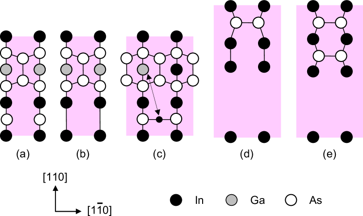
Figure 1: (Color online) Schematic diagrams of surface reconstruction models of InAs/GaAs wetting layer on GaAs(001) reproduced from literature: (a)  $(1\times 3)$ ono01 , (b)  $(1\times 3)$ kita02 , (c)  $(2\times 3)$ ishii03 , (d)  $\alpha 2(2\times 4)$ yamaguchi95 ; carter02 , (e)  $\beta 2(2\times 4)$ yamaguchi95 ; carter02 . Background shade indicates unit cell.

The distribution of reconstruction domains and QD nucleation sites is characterized by spatial point patterns; that is a regular (ordered) pattern, a Poisson (random) pattern, and a clustered (aggregated) pattern diggle03 ; osullivan03 . In a regular pattern, points are distributed uniformly. A Voronoi tessellation, that is polygonal decomposition of a space by perpendicular bisector lines among neighboring points, is often used in spatial point analysis. The standard deviation of Voronoi cell area, $\sigma_{\mathrm{Vc}}$, represents point patterns. Here, we have to be careful of the Voronoi cells touching the boundary of the study region because of “edge effect” that contribution from points outside cannot be taken into account. In this study, such invalid Voronoi cells were excluded from the study region. For more precise analysis, second-order properties of point patterns like nearest-neighbor distances are useful osullivan03 ; tanemura81 ; ogata81 ; baddeley97 . Let $r$ denote the distance to the nearest point from a randomly selected location in the study region $R$. The $F(d)$ function denotes the cumulative frequency distribution of $r$ osullivan03 and hence the probability that $r$ occurs less than any particular distance $d$. Since the $F$ function is practically identical to the probability of plotting a random point within any of circles $C_{i}(d)$, of each radius $d$, centered on each of the points, it is simply computed by

$$F(d)=\frac{\mathrm{Area}\left(\bigcup_{i}C_{i}(d)\cap R\right)}{\mathrm{Area}\left(R\right)},$$ (1)

where the numerator is the area of the union of the circles, and the denominator is the area of the study region $R$. To compare $F(d)$ between different study regions, $d$ should be normalized by the factor $f$ as follows:

$$f=\sqrt{\textrm{Area}\left(R\right)/N},$$ (2)

where $N$ is the number of points tanemura81 .

A piece ($11\times 13\times 0.6$ mm³) of GaAs(001) crystal was used as a substrate. First the surface was thermally cleaned to remove the oxide layer under $1\times 10^{-4}$ Pa of an As₄ atmosphere in an MBE growth chamber. Next, a GaAs buffer layer was grown on the surface by using MBE until atomically smooth surface was obtained. The substrate was annealed at 430$\,{}^{\circ}\mathrm{C}$ for 0.5 h to confirm the formation of $c(4\times 4)$ reconstruction with RHEED. An STM unit was transferred to the sample holder in the growth chamber and started scanning. This means that the sample was neither cooled to room temperature nor exposed to air to be observed with STM. The tip bias was -3 V and the tunnel current was 0.2 nA. A flux of In was irradiated at the InAs growth rate of $2.5\times 10^{-4}$ MLs^-1. After 1.5 monolayer (ML) of InAs WL growth, the substrate temperature was decreased to 300$\,{}^{\circ}\mathrm{C}$ and the As₄ flux was shut off so that the surface reconstruction should be observed in an atomic scale. Another samples was prepared in the same way but SK growth of InAs WL was continued at 430$\,{}^{\circ}\mathrm{C}$ until QD precursors were formed tsukamoto06 . An STM image of QD precursors was recorded to analyze the distribution of QD nucleation sites.

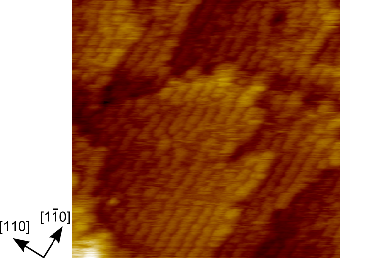
Figure 2: (Color) 30 nm $\times$ 30 nm filled-state STM image of InAs WL on GaAs(001).

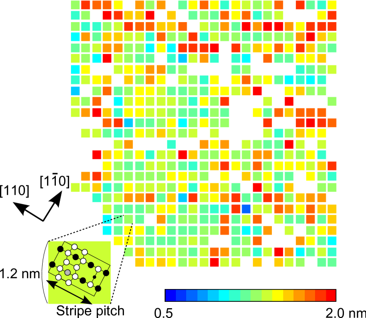
Figure 3: (Color) Map of As-dimer stripe pitch along [110] azimuth measured in each cell of $25\times 25$ mesh in Fig. 2. Schematic diagram of magnified mesh cell is also illustrated aside to show the relationship between stripe pitch measured and corresponding unit cell of InAs WL surface reconstruction in Fig. 1.

Figure 2 shows the filled-state STM image of 1.5 ML of InAs WL recorded at 300$\,{}^{\circ}\mathrm{C}$. The image seems more or less scratched because of migrating In adatoms on the surface but shows the stripes due to As dimers clearly enough to measure the pitch. The stripe pitch corresponds to the unit cell length along [110] azimuth of InAs WL surface reconstructions in Fig. 1. Although it is difficult to discuss the unit cell size of strained and mixed surface reconstructions, it is expected to have some intermediate value between those of GaAs and InAs. We assumed that the stripe pitch along [110] azimuth ranged 0.6–1.0 nm for $c(4\times 4)$, 1.0–1.4 nm for $(1\times 3)/(2\times 3)$, and 1.4–2.0 nm for $(2\times 4)$. Before measuring the stripe pitch, the STM image [Fig. 2] was divided by a $25\times 25$ mesh. As shown in the schematic diagram in Fig. 3, the size of each mesh cell is 1.2 nm which is comparable to the unit cell sizes of the InAs WL surface reconstructions. The stripe pitch was measured from the STM line profile along [110] azimuth for each mesh cell. The data are plotted in the color map of Fig. 3. Most cells show $(1\times 3)/(2\times 3)$ or $(2\times 4)$ surface reconstruction although some cells are blank because of step edges.

It is predicted that Ga-rich fluctuation, comprised of at least eight Ga atoms in an In/Ga mixing layer, should be a QD nucleation site according to kMC simulations tsukamoto06 . For such Ga-rich fluctuation to be formed, four unit cells of $(1\times 3)/(2\times 3)$ need to be contiguous, each of which has one or two Ga atoms. In this study, groups of four neighboring mesh cells, having the same surface reconstruction, were located in the map [Fig. 3] and indicated by oval markers in Fig. 4. For each of $(1\times 3)/(2\times 3)$ and $(2\times 4)$ surface reconstructions, the centroid points of the domains were marked and their coordinates were measured by using ImageJ software rasband09 ; abramoff04 . The centroid coordinates were used for the Voronoi tessellations of the reconstruction domain maps [Fig. 4] and computation of the $F$ function tanemura81 .

Figure 5 shows the 150 nm $\times$ 150 nm STM image of InAs QD precursors immediately after nucleation tsukamoto06 . The STM image was divided into 3 $\times$ 3 regions. For each region, measurement of QD coordinates, a Voronoi tessellation, and computation of the $F$ function were performed as well.

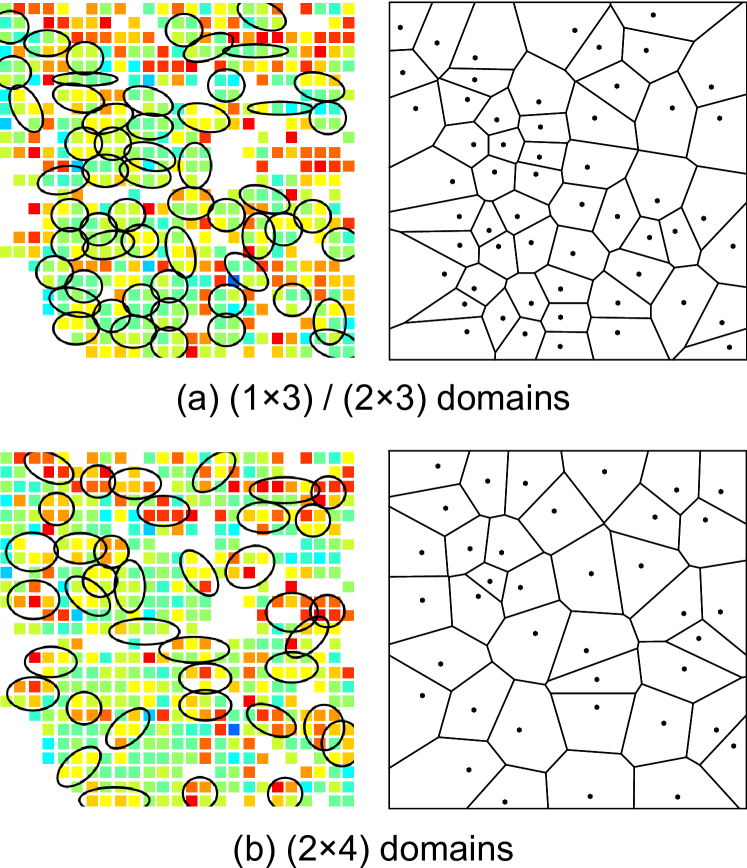
Figure 4: (Color) Surface reconstruction domains, indicated by oval markers, and Voronoi tessellations of (a) $(1\times 3)/(2\times 3)$ and (b) $(2\times 4)$ surface reconstruction maps.

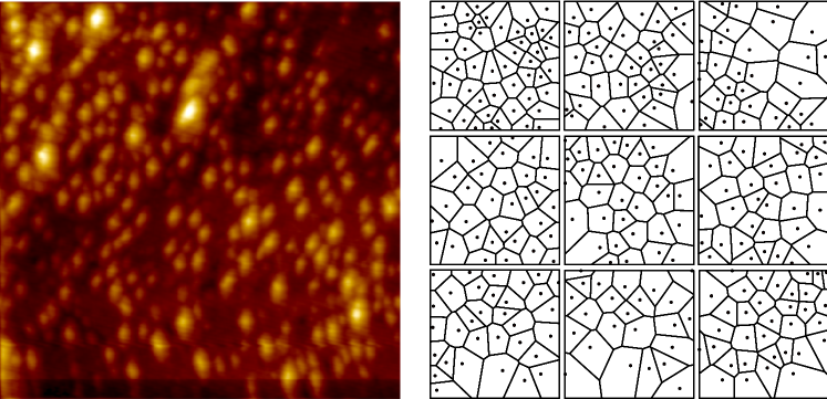
Figure 5: (Color) 150 nm $\times$ 150 nm STM image of QD precursors nucleated on SK grown InAs WL at 430$\,{}^{\circ}\mathrm{C}$ tsukamoto06 and Voronoi tessellations computed for each of 3 $\times$ 3 regions.

Table 1: Density $\rho$ and standard deviation of Voronoi cell area $\sigma_{\mathrm{Vc}}$ of surface reconstruction domains and QD precursors.

	$\rho$ ($10^{12}$ cm-2)	$\sigma_{\mathrm{Vc}}$
$(1\times 3)/(2\times 3)$ domains	6.2	0.38
$(2\times 4)$ domains	4.2	0.31
QD precursors	0.96–1.7	0.20–0.59

Table. 1 lists the density and standard deviation of valid Voronoi cells computed for the surface reconstruction domains in Fig. 4 and the QD precursors in Fig. 5. Each standard deviation is normalized by each study region area. For QD precursors, the minimum and maximum data in the nine regions are shown. The densities of surface reconstruction domains were similar to those of QD precursors. The standard deviations of surface reconstruction domains were in the range of QD precursors. The similarity in these properties implies some relationship between surface reconstruction domains and QD precursors.

The $F$ function will give more precise information. Figure 6 shows the $F(d)$ traces calculated for the surface reconstruction domains [ 4] and the $F(d)$ envelope of the QD precursors [ 5]. The $F(d)$ envelope of typical Poisson patterns was calculated by accumulating 50 simulations of scattering 50 random points.

Both traces of $(1\times 3)/(2\times 3)$ and $(2\times 4)$ domains were similar to the envelope of QD precursors although they differs in the detail. The traces of the surface reconstruction domains and the QD precursors were plotted between those of the ordered pattern and the Poisson patterns. This shows that surface reconstruction domains and QD precursors are distributed in a rather ordered pattern than a random pattern. An ordered pattern likely occurs when there is repulsive force among points. It is difficult to discuss the origin of repulsive force by STM images, one can consider the surface strain distribution. First principles calculations of WL would give some insights for the surface stain distribution. It is possible that the uniformity of QD nucleation, which is rather ordered, is originated from the distribution of surface reconstruction domains.

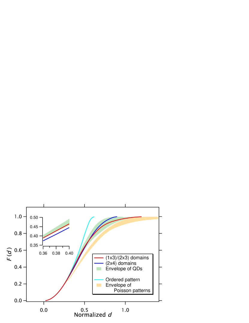
Figure 6: (Color) Traces of $F$ functions of surface reconstruction domains and typical ordered point pattern. Envelope regions of QDs in nine regions and typical Poisson patterns by accumulating 50 simulations are also shown. Magnified view of region where $d$ is 0.36 to 0.40 is superimposed.

The trace of $(2\times 4)$ domains is located rather ordered in the QD envelope, and completely deviates from the QD envelope in small $d$ region as can be seen in the magnified view in Fig. 6. The trend of $F(d)$ where $d$ is small is dependent on the pattern in dense-point areas. On the other hand, the trend of $F(d)$ where $d$ is large is dependent on the pattern in sparse-point areas. The pattern in dense-point areas is particularly crucial because of high surface strain which severely affects the distribution. In the sense of not deviating in dense-point areas, the trace of $(1\times 3)/(2\times 3)$ domains represents the QD precursor envelope better than that of $(2\times 4)$ domains. In other words, the distribution of QD precursors are more similar to that of $(1\times 3)/(2\times 3)$ domains than that of $(2\times 4)$ domains. The similarity in the density and the point pattern implies that QD nucleation is related to $(1\times 3)/(2\times 3)$ domains where Ga-rich fluctuation is assumed to be formed. This also means that QD nucleation sites are already determined at the time when InAs WL is grown to 1.5 ML or before.

In conclusion, we have shown, by using in situ STM, the similarity in the density and the spatial point patterns between $(1\times 3)/(2\times 3)$ surface reconstruction domains on 1.5 ML of SK grown InAs WL and QD precursors nucleated. This implies that QD nucleation site is related to the distribution of $(1\times 3)/(2\times 3)$ domains at the stage of 1.5 ML-grown InAs WL. Since a $(1\times 3)/(2\times 3)$ domain composed of four unit cells is assumed to contain Ga-rich fluctuation with at least eight Ga atoms, this model provides a consistent evidence that QD nucleation is induced by tiny alloy fluctuation as predicted by kMC simulations tsukamoto06 . The mechanism of QD nucleation, exhibited here, has important technological implications for the self-assembly and the artificial arrangement of QDs.

- (1) Y. Arakawa and H. Sakaki, Appl. Phys. Lett. 40, 939 (1982)
- (2) S.-S. Li, J.-B. Xia, J.-L. Liu, F.-H. Yang, Z.-C. Niu, S.-L. Feng, and H.-Z. Zheng, J. Appl. Phys. 90, 6151 (2001)
- (3) A. Fiore, C. Zinoni, B. Alloing, C. Monat, L. Balet, L. H. Li, N. L. Thomas, R. Houdré, L. Lunghi, M. Francardi, A. Gerardino, and G. Patriarche, J. Phys.: Condens. Matter 19, 225005 (2007)
- (4) P. M. Intallura, M. B. Ward, O. Z. Karimov, Z. L. Yuan, P. See, P. Atkinson, D. A. Ritchie, and A. J. Shields, J. Opt. A: Pure Appl. Opt. 11, 054005 (2009)
- (5) P. Kratzer, E. Penev, and M. Scheffler, Appl. Surf. Sci. 216, 436 (2003)
- (6) A. Ishii, K. Fujiwara, and T. Aisaka, Appl. Surf. Sci. 216, 478 (2003)
- (7) K. Fujiwara, A. Ishii, and T. Aisaka, Thin Solid Films 464–465, 35 (2004)
- (8) A. Ishii, M. Tsukao, N. Toda, and S. Oshima, e-print arXiv:cond-mat/0501233 (2005)
- (9) S. Tsukamoto, T. Honma, G. R. Bell, A. Ishii, and Y. Arakawa, small 2, 386 (2006)
- (10) J. G. Belk, J. L. Sudijono, D. M. Holmes, C. F. McConville, and T. S. Jones, Surf. Sci. 365, 735 (1996)
- (11) J. G. Belk, C. F. McConville, J. L. Sudijono, T. S. Jones, and B. A. Joyce, Surf. Sci. 387, 213 (1997)
- (12) T. J. Krzyzewski, P. B. Joyce, G. R. Bell, and T. S. Jones, Surf. Sci. 482–485, 891 (2001)
- (13) S. Tsukamoto and N. Koguchi, J. Cryst. Growth 201–202, 118 (1999)
- (14) K. Ono, T. Mano, K. Nakamura, M. Mizuguchi, H. Kiwata, S. Nakazono, K. Horiba, T. Kihara, J. Okabayashi, A. Kakizaki, and M. Oshima, Abstracts of ICCG-13/ICVGE-11, Kyoto, 402(2001)
- (15) T. Kita, O. Wada, T. Nakayama, and M. Murayama, Phys. Rev. B 66, 195312 (2002)
- (16) H. Yamaguchi and Y. Horikoshi, J. Cryst. Growth 150, 148 (1995)
- (17) W. Barvosa-Carter, R. S. Ross, C. Ratsch, F. Grosse, J. H. G. Owen, and J. J. Zinck, Surf. Sci. 499, L129 (2002)
- (18) P. J. Diggle, Statistical Analysis of Spatial Point Patterns (Oxford University Press, Inc., New York, 2003)
- (19) D. O’Sullivan and D. J. Unwin, Geographic Information Analysis (John Wiley & Sons, Inc., New Jersey, 2003)
- (20) M. Tanemura and Y. Ogata, Suuri Kagaku (Mathematical Sciences) 213, 11 (1981)
- (21) Y. Ogata and M. Tanemura, Ann. Inst. Statist. Math. 33, 315 (1981)
- (22) A. Baddeley and R. D. Gill, Ann. Statist. 25, 263 (1997)
- (23) W. J. Rasband, “ImageJ,” U. S. National Institutes of Health, Bethesda, Maryland, USA (1997–2009), http://rsb.info.nih.gov/ij/
- (24) M. D. Abramoff, P. J. Magelhaes, and S. J. Ram, Biophotonics Int. 11, 36 (2004)