Adaptive non-asymptotic confidence balls in density estimation.

Matthieu Lerasle111Instituto de Matemรกtica e Estatรญstica -USP Granted by Fapesp Processo 2009/09494-0,

Abstract:

We build confidence balls for the common density s๐‘ s of a real valued sample $X_{1},...,X_{n}$. We use resampling methods to estimate the projection of s๐‘ s onto finite dimensional linear spaces and a model selection procedure to choose an optimal approximation space. The covering property is ensured for all $n\geq 2$ and the balls are adaptive over a collection of linear spaces.

Key words: Confidence balls, density estimation, resampling methods.

2000 Mathematics Subject Classification: 62G07, 62G09, 62G10, 62G15.

1 Introduction

In this paper, we discuss the problem of adaptive confidence balls, from a non-asymptotic point of view, in the particular context of density estimation. Let $S$ be a set of densities with respect to the Lebesgue measure $\mu$ on $\mathbb{R}$. Given an i.i.d sample $X_{1:n}=(X_{1},...,X_{n})$ and a confidence level $\beta\in(0,1)$, a confidence set (hereafter CS) $\hat{B}_{\beta}(X_{1:n})$ on $S$ is a subset of $S$ satisfying the following covering property:

โˆ€sโˆˆS,โ„™sโ€‹(sโˆˆB^ฮฒโ€‹(X1:n))โ‰ฅ1โˆ’ฮฒformulae-sequencefor-all๐‘ ๐‘†subscriptโ„™๐‘ ๐‘ subscript^๐ต๐›ฝsubscript๐‘‹:1๐‘›1๐›ฝ\forall s\in S,\;\mathbb{P}_{s}\left(s\in\hat{B}_{\beta}(X_{1:n})\right)\geq 1-\beta (1)

where, for all s๐‘ s in $S$, โ„™ssubscriptโ„™๐‘ \mathbb{P}_{s} denotes the distribution of $X_{1:n}$ when the marginals have common density s๐‘ s. All the CS considered in this paper are $L^{2}$-balls, centered on estimators s^^๐‘ \hat{s} of s๐‘ s, and with random radius $\hat{\rho}_{\beta}$. The quality of a CS is measured with the quantiles of $\hat{\rho}_{\beta}$. We are looking for adaptive CS, which means that, given a collection $(S_{m})_{m\in\mathcal{M}_{n}}$ of subsets of $S$, $\hat{\rho}_{\beta}$ should be as small as possible over all the sets $(S_{m})_{m\in\mathcal{M}_{n}}$.
This problem was mostly considered in regression frameworks, see among others Li [25], Lepski [23], Juditski $\&$ Lepski [20], Hoffmann $\&$ Lepski [14], Juditski $\&$ Lambert-Lacroix [19], Baraud [4], Beran [5], Beran $\&$ Dรผmbgen [6], Cai $\&$ Low [9], Genovese $\&$ Wassermann [12, 13]. Robins $\&$ van der Vaart [28] considered a more general Hilbertian framework that includes in particular density estimation and some regression frameworks.
Our adaptive balls are derived from a model selection procedure, which is essentially the one of Baraud [4]. We start with a collection of linear spaces $(S_{m})_{m\in\mathcal{M}_{n}}$ and associate to each of these, the projection estimator s^msubscript^๐‘ ๐‘š\hat{s}_{m} of s๐‘ s and some positive number $\hat{\rho}(m)$. The $\hat{\rho}(m)$โ€™s are suitably calibrated to satisfy the property that, with probability close to one the distance between s๐‘ s and its projection estimator s^msubscript^๐‘ ๐‘š\hat{s}_{m} is not larger than $\hat{\rho}(m)$. We then select $\hat{m}$ as the minimizer of $\hat{\rho}(m)$ and define the confidence ball as the $L^{2}$-ball centered at s^m^subscript^๐‘ ^๐‘š\hat{s}_{\hat{m}} of radius $\hat{\rho}(\hat{m})$.
We use two different ingredients to compute $\hat{\rho}(m)$. The first one is a resampling estimator of โ€–smโˆ’s^mโ€–2superscriptnormsubscript๐‘ ๐‘šsubscript^๐‘ ๐‘š2\|s_{m}-\hat{s}_{m}\|^{2}, where smsubscript๐‘ ๐‘šs_{m} denotes the projection of s๐‘ s onto $S_{m}$. It is naturally derived from Efronโ€™s heuristic (see Efron [10]), in the same way as Arlot, Blanchard $\&$ Roquain [2]. This allows us in particular to keep all the sample to build s^msubscript^๐‘ ๐‘š\hat{s}_{m}. This is an improvement compared with Robins $\&$ van der Vaart [28] or Cai $\&$ Low [9], who cut the sample into two parts, the first one being used to build an estimator s^^๐‘ \hat{s} of s๐‘ s and the other to evaluate the distance โ€–s^โˆ’sโ€–2superscriptnorm^๐‘ ๐‘ 2\|\hat{s}-s\|^{2}.
The second ingredient is an estimator of โ€–sโˆ’smโ€–2superscriptnorm๐‘ subscript๐‘ ๐‘š2\|s-s_{m}\|^{2}, based on U-statistics, as in Laurent [21, 22]. The proofs are handled thanks to a concentration inequality for $U$-statistics, derived from Houdrรฉ &\& Reynaud-Bouret [15]. The main advantage of a model selectionโ€™s approach is that the resulting CS are non asymptotic, i.e. (1) holds for all $n$. Moreover, the CS behaves well even if s๐‘ s does not belong to $S$, which outperforms, in that case, the result of Li [25].
Let $S$ be a linear space with dimension $d$ and let $(S_{m})_{m\in\mathcal{M}_{n}}$ be a collection of linear subspaces of $S$, with respective dimensions $(d_{m})_{m\in\mathcal{M}_{n}}$. The diameter of our CS on $S$ is upper bounded, for any s๐‘ s in $S_{m}$, by $C(\sqrt{d}\vee d_{m})/n$, where $C$ is a constant, free from $d$, $d_{m}$, and $n$. This bound is optimal in the minimax sense. Hence, adaptation is possible over collections of subspaces with dimension $d_{m}\geq\sqrt{d}$ for $L^{2}$-balls. This positive result does not hold in general, in particular, adaptation is impossible for $L^{\infty}$-balls (Low [26]). However, the adaptation property is strongly limited since it is impossible over spaces with dimension $d_{m}\leq\sqrt{d}$. This negative result was already proved asymptotically in Li [25], Hoffmann $\&$ Lepski [14], Juditski $\&$ Lambert-Lacroix [19], Robins $\&$ van der Vaart [28]. It was proved non-asymptotically in a regression framework in Baraud [4]. We use the method of Baraud [4] and extend his result to the density estimation framework.
The paper is decomposed as follows. Section 2 introduces the notations and the main assumptions. Section 3 presents the technical tools required for the construction of our CS. Section 4 gives the main results, we build our CS, give upper bounds on their size and prove their optimality in the minimax sense. Section 5 presents a short simulation study, where we illustrate the behavior of our resampling-based estimators. All the proofs are postponed to Section 6. We add in an Appendix the proofs of some technical lemmas.

2 Notations and assumptions

2.1 Notations

Hereafter, $L^{2}(\mu)$ denotes the space of all measurable functions $t:\mathbb{R}\rightarrow\mathbb{R}$ such that $\int_{\mathbb{R}}t^{2}(x)d\mu(x)<\infty$. It is endowed by its classical scalar product defined, for all $t$, $t^{\prime}$ in $L^{2}(\mu)$ by $<t,t^{\prime}>=\int_{\mathbb{R}}t(x)t^{\prime}(x)d\mu(x)$ and by the associated $L^{2}$-norm defined, for $t$ in $L^{2}(\mu)$ by $\|t\|=\sqrt{<t,t>}.$
For any density s๐‘ s, we denote by โ„™ssubscriptโ„™๐‘ \mathbb{P}_{s} the distribution of an iid sample $X_{1:n}=(X_{1},...,X_{n})$ with common marginal density s๐‘ s and by ๐”ผssubscript๐”ผ๐‘ \mathbb{E}_{s} the expectation with respect to โ„™ssubscriptโ„™๐‘ \mathbb{P}_{s}.
Hereafter, $S$, with various subscripts, denotes a linear subspace of $L^{2}(\mu)$ and $S^{*}$ the set of densities in $S$. For all sets $\mathcal{F}$ in $L^{2}(\mu)$, the $L^{2}$-diameter of $\mathcal{F}$ is defined by

$$\Delta(\mathcal{F})=\sup_{(t,t^{\prime})\in\mathcal{F}^{2}}\|t-t^{\prime}\|.$$

For a random set $\hat{B}$ in $L^{2}(\mu)$, a linear space $S$ of measurable functions and a real number $\alpha$ in $(0,1)$, we define the $(S,\alpha)$-size of $\hat{B}$ as

ฮ”(S,ฮฑ)โ€‹(B^)=inf{ฮด>0,supsโˆˆSโˆ—โ„™sโ€‹(ฮ”โ€‹(B^)>ฮด)โ‰คฮฑ}.subscriptฮ”๐‘†๐›ผ^๐ตinfimumformulae-sequence๐›ฟ0subscriptsupremum๐‘ superscript๐‘†subscriptโ„™๐‘ ฮ”^๐ต๐›ฟ๐›ผ\Delta_{(S,\alpha)}(\hat{B})=\inf\left\{\delta>0,\;\sup_{s\in S^{*}}\mathbb{P}_{s}(\Delta(\hat{B})>\delta)\leq\alpha\right\}. (2)

For all indexes sets $\Lambda$, $(\psi_{\lambda})_{\lambda\in\Lambda}$ will always denote an orthonormal system in $L^{2}(\mu)$.

2.2 Efronโ€™s resampling heuristic

Let $X,X_{1},...,X_{n}$ be i.i.d random variables with common density s๐‘ s, let Pssubscript๐‘ƒ๐‘ P_{s} and $P_{n}$ denote the following processes defined respectively for all functions $t$ in $L^{2}(\mu)$ and for all measurable functions $t$ by

$$P_{s}t=<s,t>=\int_{\mathbb{R}}t(x)s(x)d\mu(x)=\mathbb{E}(t(X)),\;P_{n}t=\frac{1}{n}\sum_{i=1}^{n}t(X_{i}).$$

Hereafter, a resampling scheme $(W_{1},...,W_{n})$ is a vector of real valued random variables, independent of $(X_{1},....,X_{n})$ and exchangeable, which means that, for all permutations $\tau$ of $1,...,n$,

$$(W_{\tau(1)},...,W_{\tau(n)})\;{\rm has}\;{\rm the}\;{\rm same}\;{\rm law}\;{\rm as}\;(W_{1},...,W_{n}).$$

Let $(W_{1},...,W_{n})$ be a resampling scheme, let $\bar{W}_{n}=\sum_{i=1}^{n}W_{i}/n$ and let $P_{n}^{W}$ denotes the resampling-based empirical process defined, for all measurable functions $t$, by

$$P_{n}^{W}t=\frac{1}{n}\sum_{i=1}^{n}W_{i}t(X_{i}).$$

For all random variables $F(X_{1},...,X_{n},W_{1},...,W_{n})$, we denote by

$$\mathbb{E}_{W}\left(F(X_{1},...,X_{n},W_{1},...,W_{n})\right)=\mathbb{E}\left(F(X_{1},...,X_{n},W_{1},...,W_{n})|X_{1},...,X_{n}\right).$$

Let $F$ be a known functional and Fn=Fโ€‹(Pn,Ps)subscript๐น๐‘›๐นsubscript๐‘ƒ๐‘›subscript๐‘ƒ๐‘ F_{n}=F(P_{n},P_{s}), we define the resampling estimator of $F_{n}$ by

$$F_{n}^{W}=C_{W}\mathbb{E}_{W}\left(F(P_{n}^{W},\bar{W}_{n}P_{n})\right),$$

where $C_{W}$ is a constant depending only on the functional $F$ and the law of the resampling scheme. Efronโ€™s heuristics states that $F_{n}^{W}$ provides a sharp estimator of $F_{n}$ when the constant $C_{W}$ is well chosen.

2.3 Balls in functional spaces

Our method is strongly based on empirical process methods, in particular on Talagrandโ€™s concentration inequality. This inequality involves some $L^{\infty}$-norms, this is why we introduce the following notations. Let $S$ be a linear space of measurable functions. For any function $t$ in $L^{2}(\mu)\cap L^{\infty}(\mu)$, let $\pi_{S}(t)$ denote its orthogonal projection onto $S$, let $\left\|t\right\|_{\infty}$ be its $L^{\infty}$-norm. For all $C$, $C^{\prime}$, $\eta$ in $\bar{\mathbb{R}}_{+}$, for all $t$ in $L^{2}(\mu)$, let

$$B_{2}(t,C,S)=\{t^{\prime}\in S,\;\|t^{\prime}-t\|\leq C\},\;B(S)=B_{2}(0,1,S)=\left\{t\in S,\;\|t\|\leq 1\right\}.$$ (3)
$$B_{2,\infty}(C,C^{\prime},\eta,S)=\left\{t\in L^{2}(\mu)\cap L^{\infty}(\mu),\;\|t\|\leq C,\;\left\|t\right\|_{\infty}\leq C^{\prime},\;\|t-\pi_{S}(t)\|\leq\eta\right\}.$$ (4)

2.4 Basic definitions

Definition 2.1.

(Confidence Sets)
Let $(X_{1},...,X_{n})$ be an i.i.d. sample of real valued random variables, let $S\subset L^{2}(\mu)$ and let $\beta$ be a real number in $(0,1)$. The set $CS(S,\beta)$ of $(1-\beta)$-confidence balls on $S$ is defined as the collection of all subsets B^ฮฒ=B2โ€‹(s^,ฯ^ฮฒ,S)subscript^๐ต๐›ฝsubscript๐ต2^๐‘ subscript^๐œŒ๐›ฝ๐‘†\hat{B}_{\beta}=B_{2}(\hat{s},\hat{\rho}_{\beta},S) of $L^{2}(\mu)$, where s^^๐‘ \hat{s} and $\hat{\rho}_{\beta}$ are measurable with respect to $\sigma(X_{1},...,X_{n})$ such that

โˆ€sโˆˆSโˆ—,โ„™sโ€‹(sโˆˆB^ฮฒ)โ‰ฅ1โˆ’ฮฒ.formulae-sequencefor-all๐‘ superscript๐‘†subscriptโ„™๐‘ ๐‘ subscript^๐ต๐›ฝ1๐›ฝ\forall s\in S^{*},\;\mathbb{P}_{s}\left(s\in\hat{B}_{\beta}\right)\geq 1-\beta.
Definition 2.2.

(Minimax rate of convergence for confidence sets)
Let $(X_{1},...,X_{n})$ be an i.i.d. sample of real valued random variables, let $S^{\prime}\subset S\subset L^{2}(\mu)$ and let $\alpha$, $\beta$ be real numbers in $(0,1)$. The $(\alpha,\beta)$-minimax rate of convergence over $S^{\prime}$ for CS on $S$ is defined as

$$\phi_{n}(\alpha,\beta,S,S^{\prime})=\inf_{\hat{B}_{\beta}\in CS(S,\beta)}\Delta_{(S^{\prime},\alpha)}(\hat{B}_{\beta}).$$
Definition 2.3.

(Adaptive confidence sets)
Let $(X_{1},...,X_{n})$ be an i.i.d. sample of real valued random variables, let $S\subset L^{2}(\mu)$, let $(S_{m})_{m\in\mathcal{M}_{n}}$ be a collection of subsets of $S$ and let $\alpha$, $\beta$ be real numbers in $(0,1)$. A CS $\hat{B}_{\beta}$ in $CS(S,\beta)$ is said to be optimal, or adaptive over $(S_{m})_{m\in\mathcal{M}_{n}}$, if the following condition holds.
For all fixed $\alpha$ in $(0,1)$, there exists a constant $c(\alpha,\beta)>0$ free from $n$, $S$ and $(S_{m})_{m\in\mathcal{M}_{n}}$ such that, for all $m$ in $\mathcal{M}_{n}$,

$$\Delta_{S_{m},\alpha}(\hat{B}_{\beta})\leq c(\alpha,\beta)\phi_{n}(\alpha,\beta,S,S_{m})$$
Definition 2.4.

(Test)
Let $(X_{1},...,X_{n})$ be an i.i.d. sample of real valued random variables. Let $S$ be a family of densities on $\mathbb{R}$. Let $S_{0}$, $S_{1}$ be two disjoint subsets in $S$. A test $T$ of the assumption H0:sโˆˆS0:subscript๐ป0๐‘ subscript๐‘†0H_{0}:s\in S_{0} against the alternative H1:sโˆˆS1:subscript๐ป1๐‘ subscript๐‘†1H_{1}:s\in S_{1} is a function $T:\mathbb{R}^{n}\rightarrow\{0,1\}$. The test $T$ is said to have a confidence level $1-\alpha\in(0,1)$ when

โˆ€sโˆˆS0,โ„™sโ€‹(Tโ€‹(X1,โ€ฆ,Xn)=0)โ‰ฅ1โˆ’ฮฑ.formulae-sequencefor-all๐‘ subscript๐‘†0subscriptโ„™๐‘ ๐‘‡subscript๐‘‹1โ€ฆsubscript๐‘‹๐‘›01๐›ผ\forall s\in S_{0},\;\mathbb{P}_{s}\left(T(X_{1},...,X_{n})=0\right)\geq 1-\alpha.

It is said to have a power $1-\beta\in(0,1)$ when

โˆ€sโˆˆS1,โ„™sโ€‹(Tโ€‹(X1,โ€ฆ,Xn)=1)โ‰ฅ1โˆ’ฮฒ.formulae-sequencefor-all๐‘ subscript๐‘†1subscriptโ„™๐‘ ๐‘‡subscript๐‘‹1โ€ฆsubscript๐‘‹๐‘›11๐›ฝ\forall s\in S_{1},\;\mathbb{P}_{s}\left(T(X_{1},...,X_{n})=1\right)\geq 1-\beta.

2.5 Main Assumptions

Let $(S_{m})_{m\in\mathcal{M}_{n}}$ be a collection of linear subspaces of $L^{2}(\mu)$, with finite dimensions respectively denoted by $(d_{m})_{m\in\mathcal{M}_{n}}$. We make the following assumptions on this collection.
H1: There exists $m_{n}$ in $\mathcal{M}_{n}$ such that $S_{m_{n}}={\rm Span}\left(\bigcup_{m\in\mathcal{M}_{n}}S_{m}\right)$.
H2: There exists a constant $C_{1}$ such that, for all $m$ in $\mathcal{M}_{n}$, for all $t$ in $S_{m}$

$$\left\|t\right\|_{\infty}\leq C_{1}\sqrt{d_{m}}\|t\|.$$

The last assumption is only technical and let us simplify the results. Let $\beta$ be a real number in $(0,1)$.
H3$(\mathcal{M},\beta)$: For all $n\geq 2$ $N_{n}={\rm Card}(\mathcal{M}_{n})$ is finite and there exists a constant $C_{\mathcal{M}}$ such that, for all $n\geq 2$,

$$\frac{2\sqrt{d_{n}}\ln(6N_{n}/\beta)}{n}\leq C_{\mathcal{M}}.$$

Four examples are usually developed as fulfilling this set of assumptions:
[Hist] regular histogram spaces: for all $m$ in $\mathbb{N}^{*}$, $S_{m}$ is the space of all the functions constant on the partition $(I_{[k/m,(k+1)/m)})_{k=0,...,m-1}$ of $[0,1]$, $d_{m}=m$.
[T] trigonometric spaces: $S_{m}$ is the linear span of the functions $\psi_{0,0}(x)=1_{[0,1]}$, $\psi_{j,1}(x)=\sqrt{2}\cos(2\pi jx)1_{[0,1]}(x)$ and $\psi_{j,2}(x)=\sqrt{2}\sin(2\pi jx)1_{[0,1]}(x)$ for all $1\leq j\leq J_{m}$. $d_{m}=2J_{m}+1$.
[P] regular piecewise polynomial spaces: $S_{m}$ is the linear span of the functions $(\psi_{j,k})$ for $j=1,...,J_{m}$, $k=0,...,r-1$, where, for all $j=1,...,J_{m}$ and $k=0,...,r-1$, $\psi_{j,k}$ is a polynomial of degree $k$ on $[(j-1)/J_{m},j/J_{m}]$. $d_{m}=rJ_{m}$.
[W] spaces spanned by dyadic wavelets with regularity $r$.
We have to choose $d_{m_{n}}\leq Cn^{2}/(\ln n)^{2}$ and $\beta\geq n^{-r}$ for some $r>0$ in order to fulfill Assumption H3$(\mathcal{M},\beta)$. For a description of those spaces and their properties, we refer to Birgรฉ &\& Massart [7]. Hereafter, in order to simplify the notations, we will often write $S_{n}$, $d_{n}$, snsubscript๐‘ ๐‘›s_{n},โ€ฆ instead of $S_{m_{n}}$, $d_{m_{n}}$, smnsubscript๐‘ subscript๐‘š๐‘›s_{m_{n}},โ€ฆ

3 Technical tools

This section presents the results required in Section 4 to build our adaptive confidence sets. Let s๐‘ s be a density in $L^{2}(\mu)$ and let smsubscript๐‘ ๐‘šs_{m} and snsubscript๐‘ ๐‘›s_{n} denote respectively its orthogonal projections onto the linear spaces $S_{m}$ and $S_{n}$, where $S_{m}\subset S_{n}$. We recall the definition and some basic properties of the projection estimator s^msubscript^๐‘ ๐‘š\hat{s}_{m} of s๐‘ s on $S_{m}$ in Section 3.1. From Pythagoras theorem, it satisfies

โ€–sโˆ’s^mโ€–2=โ€–sโˆ’snโ€–2+โ€–snโˆ’smโ€–2+โ€–smโˆ’s^mโ€–2.superscriptnorm๐‘ subscript^๐‘ ๐‘š2superscriptnorm๐‘ subscript๐‘ ๐‘›2superscriptnormsubscript๐‘ ๐‘›subscript๐‘ ๐‘š2superscriptnormsubscript๐‘ ๐‘šsubscript^๐‘ ๐‘š2\|s-\hat{s}_{m}\|^{2}=\|s-s_{n}\|^{2}+\|s_{n}-s_{m}\|^{2}+\|s_{m}-\hat{s}_{m}\|^{2}. (5)

Section 3.2 deals with the estimation of โ€–smโˆ’s^mโ€–2superscriptnormsubscript๐‘ ๐‘šsubscript^๐‘ ๐‘š2\|s_{m}-\hat{s}_{m}\|^{2}. We introduce our resampling estimator and state a very important concentration inequality (Theorem 3.3). In Section 3.3, we introduce our estimator of โ€–snโˆ’smโ€–2superscriptnormsubscript๐‘ ๐‘›subscript๐‘ ๐‘š2\|s_{n}-s_{m}\|^{2} based on $U$-statistics.

3.1 Projection estimators

Definition 3.1.

(projection estimators)
Let $X_{1},...,X_{n}$ be i.i.d random variables with common density s๐‘ s in $L^{2}(\mu)$. Let $S_{m}$ be a linear subspace of $L^{2}(\mu)$. The projection estimator of s๐‘ s on $S_{m}$ is defined by

s^m=inftโˆˆSmโ€–tโ€–2โˆ’2โ€‹Pnโ€‹t.subscript^๐‘ ๐‘šsubscriptinfimum๐‘กsubscript๐‘†๐‘šsuperscriptnorm๐‘ก22subscript๐‘ƒ๐‘›๐‘ก\hat{s}_{m}=\inf_{t\in S_{m}}\|t\|^{2}-2P_{n}t.

Classical computations show the following Lemma:

Lemma 3.2.

Let $X_{1},...,X_{n}$ be i.i.d random variables with common density s๐‘ s in $L^{2}(\mu)$. Let $S_{m}$ be a linear subspace of $L^{2}(\mu)$ and let $(\psi_{\lambda})_{\lambda\in\Lambda_{m}}$ be an orthonormal basis of $S_{m}$. Let smsubscript๐‘ ๐‘šs_{m} be the orthogonal projection of s๐‘ s onto $S_{m}$ and let s^msubscript^๐‘ ๐‘š\hat{s}_{m} be the projection estimator of s๐‘ s onto $S_{m}$. Then,

sm=โˆ‘ฮปโˆˆฮ›m(Psโ€‹ฯˆฮป)โ€‹ฯˆฮป,s^m=โˆ‘ฮปโˆˆฮ›m(Pnโ€‹ฯˆฮป)โ€‹ฯˆฮป,โ€–smโˆ’s^mโ€–2=โˆ‘ฮปโˆˆฮ›m[(Pnโˆ’Ps)โ€‹ฯˆฮป]2.formulae-sequencesubscript๐‘ ๐‘šsubscript๐œ†subscriptฮ›๐‘šsubscript๐‘ƒ๐‘ subscript๐œ“๐œ†subscript๐œ“๐œ†formulae-sequencesubscript^๐‘ ๐‘šsubscript๐œ†subscriptฮ›๐‘šsubscript๐‘ƒ๐‘›subscript๐œ“๐œ†subscript๐œ“๐œ†superscriptnormsubscript๐‘ ๐‘šsubscript^๐‘ ๐‘š2subscript๐œ†subscriptฮ›๐‘šsuperscriptdelimited-[]subscript๐‘ƒ๐‘›subscript๐‘ƒ๐‘ subscript๐œ“๐œ†2s_{m}=\sum_{\lambda\in\Lambda_{m}}(P_{s}\psi_{\lambda})\psi_{\lambda},\;\hat{s}_{m}=\sum_{\lambda\in\Lambda_{m}}(P_{n}\psi_{\lambda})\psi_{\lambda},\;\|s_{m}-\hat{s}_{m}\|^{2}=\sum_{\lambda\in\Lambda_{m}}\left[(P_{n}-P_{s})\psi_{\lambda}\right]^{2}.

3.2 Estimation of โ€–smโˆ’s^mโ€–2superscriptnormsubscript๐‘ ๐‘šsubscript^๐‘ ๐‘š2\|s_{m}-\hat{s}_{m}\|^{2} by resampling methods

Let s๐‘ s be a density in $L^{2}(\mu)$. Let $S_{m}$ be a finite dimensional linear subspace of $L^{2}(\mu)$, let $(\psi_{\lambda})_{\lambda\in\Lambda_{m}}$ be an orthonormal basis of $S_{m}$. Let smsubscript๐‘ ๐‘šs_{m} denote the orthogonal projection of s๐‘ s onto $S_{m}$ and let s^msubscript^๐‘ ๐‘š\hat{s}_{m} denote the projection estimator of s๐‘ s onto $S_{m}$. โ€–smโˆ’s^mโ€–2superscriptnormsubscript๐‘ ๐‘šsubscript^๐‘ ๐‘š2\|s_{m}-\hat{s}_{m}\|^{2} is a functional of $P_{n}$ and Pssubscript๐‘ƒ๐‘ P_{s}, therefore, it can be estimated by resampling. Indeed, let $(W_{1},...W_{n})$ be a resampling scheme and let $\bar{W}_{n}=\sum_{i=1}^{n}W_{i}/n$. The resampling estimator of โ€–smโˆ’s^mโ€–2superscriptnormsubscript๐‘ ๐‘šsubscript^๐‘ ๐‘š2\|s_{m}-\hat{s}_{m}\|^{2} given by Efronโ€™s heuristic (see Section 2.2) is defined for this resampling scheme and a suitably chosen constant $C_{W}$ by:

$$p_{W}(S_{m})=C_{W}\sum_{\lambda\in\Lambda_{m}}\mathbb{E}_{W}\left([(P_{n}^{W}-\bar{W}_{n}P_{n})\psi_{\lambda}]^{2}\right).$$ (6)

$p_{W}(S_{m})$ is well defined since we can check with Cauchy-Schwarz inequality that

$$p_{W}(S_{m})=C_{W}\mathbb{E}_{W}\left(\left[\sup_{t\in S_{m},\|t\|\leq 1}(P_{n}^{W}-\bar{W}_{n}P_{n})t\right]^{2}\right).$$

The deviations of $p_{W}(S_{m})$ are given by the following theorem.

Theorem 3.3.

Let $S_{m}$ be a linear subspace of $L^{2}(\mu)$ with finite dimension $d_{m}$, satisfying H2 and let $C_{3}>0$. Let $X_{1},...,X_{n}$ be an i.i.d. sample, let $(W_{1},...W_{n})$ be a resampling scheme and let $p_{W}(S_{m})$ be the associated random variables defined in (6) for $C_{W}=\left(\textrm{Var}(W_{1}-W_{n})\right)^{-1}$. There exists a constant $\kappa_{v}(C_{1},C_{3})$ such that, for all $2\leq x\leq C_{3}n/\sqrt{d_{m}}$, for all densities s๐‘ s in $L^{2}(\mu)\cap L^{\infty}(\mu)$,

โ„™sโ€‹(โ€–smโˆ’s^mโ€–2>pWโ€‹(Sm)+ฮบvโ€‹(C1,C3)โ€‹(1+โ€–sโ€–โˆžโˆงโ€–sโ€–โ€‹dm1/2โˆงdm)โ€‹dmโ€‹xn)โ‰คeโˆ’x/2.subscriptโ„™๐‘ superscriptnormsubscript๐‘ ๐‘šsubscript^๐‘ ๐‘š2subscript๐‘๐‘Šsubscript๐‘†๐‘šsubscript๐œ…๐‘ฃsubscript๐ถ1subscript๐ถ31subscriptnorm๐‘ norm๐‘ superscriptsubscript๐‘‘๐‘š12subscript๐‘‘๐‘šsubscript๐‘‘๐‘š๐‘ฅ๐‘›superscript๐‘’๐‘ฅ2\mathbb{P}_{s}\left(\|s_{m}-\hat{s}_{m}\|^{2}>p_{W}(S_{m})+\kappa_{v}(C_{1},C_{3})(1+\sqrt{\left\|s\right\|_{\infty}\wedge\left\|s\right\|d_{m}^{1/2}\wedge d_{m}})\frac{\sqrt{d_{m}}x}{n}\right)\leq e^{-x/2}.

Comments:

  • โ€ข

    This theorem is one of the main contributions of the article. It provides a sharp control of the variance term. It is the main difference with the article of Baraud who worked in a Gaussian framework and handled this term with a concentration inequality for $\chi^{2}$-statistics of Birgรฉ [Bi02]. Our new construction is more general and can be easily adapted to other frameworks, which is not the case in Baraud [4].

  • โ€ข

    It is proved thanks to a technical lemma (Lemma 6.1) and a sharp concentration inequality (Lemma 6.2). Lemma 6.1 shows that, with our choice of $C_{W}$, โ€–smโˆ’s^mโ€–2โˆ’pWโ€‹(Sm)superscriptnormsubscript๐‘ ๐‘šsubscript^๐‘ ๐‘š2subscript๐‘๐‘Šsubscript๐‘†๐‘š\|s_{m}-\hat{s}_{m}\|^{2}-p_{W}(S_{m}) is a totally degenerate $U$-statistics of order 2. Lemma 6.2 is a concentration inequality for $U$-statistics of order 2.

  • โ€ข

    The proof of Lemma 6.2 is derived from Houdrรฉ &\& Reynaud-Bouret [15], it follows mainly the one of Fromont $\&$ Laurent [11]. The main improvement compared with Fromont $\&$ Laurent [11] is that we work with general linear spaces $S_{m}$.

  • โ€ข

    The bound involves a term โ€–sโ€–โˆžโˆงโ€–sโ€–โ€‹dm1/4โˆงdmsubscriptnorm๐‘ norm๐‘ superscriptsubscript๐‘‘๐‘š14subscript๐‘‘๐‘š\sqrt{\left\|s\right\|_{\infty}}\wedge\sqrt{\left\|s\right\|}d_{m}^{1/4}\wedge\sqrt{d_{m}}. From a theoretical point of view, the term โ€–sโ€–โ€‹dm1/4โˆงdmnorm๐‘ superscriptsubscript๐‘‘๐‘š14subscript๐‘‘๐‘š\sqrt{\left\|s\right\|}d_{m}^{1/4}\wedge\sqrt{d_{m}} is useless asymptotically when โ€–sโ€–โˆžsubscriptnorm๐‘ \left\|s\right\|_{\infty} is finite. In practice the $L^{2}$-norm of s๐‘ s is often much smaller than its $L^{\infty}$-norm. Moreover, our control can also be used when โ€–sโ€–โˆžsubscriptnorm๐‘ \left\|s\right\|_{\infty}, โ€–sโ€–norm๐‘ \left\|s\right\| or both of these quantities are unknown, since $\kappa_{v}(C_{1},C_{3})$ is free from โ€–sโ€–norm๐‘ \left\|s\right\|, โ€–sโ€–โˆžsubscriptnorm๐‘ \left\|s\right\|_{\infty}.

  • โ€ข

    The condition on $x$ is not a problem in practice. We are interested in cases where $1-e^{-x/2}$ is large, therefore, $2\leq x$ will always be satisfied. Moreover, we will see in Section 4 that the assumptions H3$(\mathcal{M},\beta)$ are designed to ensure that the interesting $x$ satisfy $x\leq C_{3}n/\sqrt{d_{m}}$ provided that $C_{3}$ is sufficiently large.

  • โ€ข

    This theorem can be used to build a model selection procedure of density estimation. Actually, an ideal penalty in this problem is given by 2โ€‹โ€–smโˆ’s^mโ€–22superscriptnormsubscript๐‘ ๐‘šsubscript^๐‘ ๐‘š22\|s_{m}-\hat{s}_{m}\|^{2} and the aim of model selection is to evaluate this ideal penalty as precisely as possible. Theorem 3.3 provides such a control. This important application is discussed in detail in [24]. For an introduction to model selection, we refer to Massart [27]. The concept of ideal penalty is defined in Arlot [1].

  • โ€ข

    In order to keep the result as readable as possible, we only give the explicit form of the constant $\kappa_{v}(C_{1},C_{3})$ in the proof of Theorem 3.3.

Corollary 3.4.

Let $X_{1},...,X_{n}$ be i.i.d. real valued random variables. Let $(S_{m})_{m\in\mathcal{M}_{n}}$ be a collection of finite dimensional linear spaces satisfying H1, H2. Let $\beta\in(0,1)$ such that this collection satisfies also H3$(\mathcal{M},\beta)$ and let $M_{2}>0$, $M_{\infty}>0$. Let $(W_{1},...,W_{n})$ be a resampling scheme and let $p_{W}(S_{m})$ be the associated resampling estimator defined in Theorem 3.3. Let $\kappa_{v}(C_{1},C_{\mathcal{M}})$ be the constant defined in Theorem 3.3 for $C_{3}=C_{\mathcal{M}}$, let $x_{n}=2\ln\left(2N_{n}/\beta\right)\vee 2$ and let

$$V(m,\beta,X_{1},...,X_{n})=p_{W}(S_{m})+\kappa_{v}(C_{1},C_{\mathcal{M}})\left(1+\sqrt{M_{\infty}\wedge M_{2}d_{m}^{1/2}\wedge d_{m}}\right)\frac{\sqrt{d_{m}}x_{n}}{n}$$ (7)

Then, for all densities s๐‘ s in $L^{2}(\mu)\cap L^{\infty}(\mu)$ such that โ€–sโ€–โ‰คM2norm๐‘ subscript๐‘€2\|s\|\leq M_{2} and โ€–sโ€–โˆžโ‰คMโˆž,subscriptnorm๐‘ subscript๐‘€\left\|s\right\|_{\infty}\leq M_{\infty},

โ„™sโ€‹(โˆƒmโˆˆโ„ณn,โ€–smโˆ’s^mโ€–2>Vโ€‹(m,ฮฒ,X1,โ€ฆ,Xn))โ‰คฮฒ2.subscriptโ„™๐‘ formulae-sequence๐‘šsubscriptโ„ณ๐‘›superscriptnormsubscript๐‘ ๐‘šsubscript^๐‘ ๐‘š2๐‘‰๐‘š๐›ฝsubscript๐‘‹1โ€ฆsubscript๐‘‹๐‘›๐›ฝ2\mathbb{P}_{s}\left(\exists m\in\mathcal{M}_{n},\;\|s_{m}-\hat{s}_{m}\|^{2}>V(m,\beta,X_{1},...,X_{n})\right)\leq\frac{\beta}{2}.

Comments:

  • โ€ข

    This corollary gives a uniform upper bound $V(m,\beta,X_{1},...X_{n})$ on the variance term.

  • โ€ข

    The size of this uniform bound, in the sense of (2), is given by the following Theorem.

Theorem 3.5.

Let $X_{1},...,X_{n}$ be i.i.d. real valued random variables. Let $(S_{m})_{m\in\mathcal{M}_{n}}$ be a collection of linear spaces satisfying H1, H2. Let $\alpha$, $\beta$ be real numbers in $(0,1)$ such that this collection satisfies also H3$(\mathcal{M},\alpha)$ and H3$(\mathcal{M},\beta)$. Let $M_{2}>0$, $M_{\infty}>0$ and let $V_{m,\beta}=V(m,\beta,X_{1},...,X_{n})$ be the associated random variables defined in (7). There exists a constant $\kappa$, free from $d_{m}$, $M_{2}$, $M_{\infty}$, $\alpha$, $\beta$, such that, for all $m$ in $\mathcal{M}_{n}$,

$$\Delta^{2}_{B_{2,\infty}(M_{2},M_{\infty},0,L^{2}(\mu)),\alpha}\left(V_{m,\beta}\right)\leq\kappa\left[\frac{d_{m}}{n}+\left(1+\sqrt{M_{\infty}\wedge M_{2}d_{m}^{1/2}\wedge d_{m}}\right)\frac{\sqrt{d_{m}}}{n}\ln\left[\frac{N_{n}}{\alpha\beta}\right]\right].$$

Comments:

  • โ€ข

    For fixed confidence level $\alpha$, $\beta$, the asymptotic order of magnitude of $V_{m,\beta}$ is $d_{m}/n$ for all models with dimension $d_{m}\geq(\ln N_{n})^{2}$.

3.3 Estimation of โ€–snโˆ’smโ€–2superscriptnormsubscript๐‘ ๐‘›subscript๐‘ ๐‘š2\|s_{n}-s_{m}\|^{2}

The simple following lemma is important to understand our procedure.

Lemma 3.6.

Let $X_{1},...,X_{n}$ be i.i.d. real valued random variables with common density s๐‘ s in $L^{2}(\mu)$. Let $S_{m}\subset S_{n}$ be two linear subspaces of $L^{2}(\mu)$, with respective finite dimensions $d_{m}$ and $d_{n}$. Let smsubscript๐‘ ๐‘šs_{m} and snsubscript๐‘ ๐‘›s_{n} be the orthogonal projections of s๐‘ s respectively onto $S_{m}$ and $S_{n}$. Let $(\psi_{\lambda})_{\lambda\in\Lambda_{n}}$ be an orthonormal basis of $S_{n}$ such that $(\psi_{\lambda})_{\lambda\in\Lambda_{m}}$ is an orthonormal basis of $S_{m}$, with $\Lambda_{m}\subset\Lambda_{n}$. Then

โ€–snโˆ’smโ€–2=โˆ‘ฮปโˆˆฮ›nโˆ’ฮ›m(Psโ€‹ฯˆฮป)2=๐”ผsโ€‹(1nโ€‹(nโˆ’1)โ€‹โˆ‘iโ‰ j=1nโˆ‘ฮปโˆˆฮ›nโˆ’ฮ›mฯˆฮปโ€‹(Xi)โ€‹ฯˆฮปโ€‹(Xj))superscriptnormsubscript๐‘ ๐‘›subscript๐‘ ๐‘š2subscript๐œ†subscriptฮ›๐‘›subscriptฮ›๐‘šsuperscriptsubscript๐‘ƒ๐‘ subscript๐œ“๐œ†2subscript๐”ผ๐‘ 1๐‘›๐‘›1superscriptsubscript๐‘–๐‘—1๐‘›subscript๐œ†subscriptฮ›๐‘›subscriptฮ›๐‘šsubscript๐œ“๐œ†subscript๐‘‹๐‘–subscript๐œ“๐œ†subscript๐‘‹๐‘—\|s_{n}-s_{m}\|^{2}=\sum_{\lambda\in\Lambda_{n}-\Lambda_{m}}(P_{s}\psi_{\lambda})^{2}=\mathbb{E}_{s}\left(\frac{1}{n(n-1)}\sum_{i\neq j=1}^{n}\sum_{\lambda\in\Lambda_{n}-\Lambda_{m}}\psi_{\lambda}(X_{i})\psi_{\lambda}(X_{j})\right) (8)

Based on this kind of lemma, Laurent [21, 22] introduced the estimators based on $U$-statistics to estimate quadratic functionals of a density. These estimators were successfully used by Fromont $\&$ Laurent [11] for goodness of fit tests in a density estimation model, and by Robins $\&$ van der Vaart [28] to build adaptive confidence sets. We follow the same steps here and define, for any observation $X_{1},...X_{n}$, for all finite dimensional linear spaces $S_{m}\subset S_{n}$, for all orthonormal basis $(\psi_{\lambda})_{\lambda\in\Lambda_{n}}$ of $S_{n}$ such that $(\psi_{\lambda})_{\lambda\in\Lambda_{m}}$ is an orthonormal basis of $S_{m}$, with $\Lambda_{m}\subset\Lambda_{n}$,

pbโ€‹(Sm,Sn)=1nโ€‹(nโˆ’1)โ€‹โˆ‘iโ‰ j=1nโˆ‘ฮปโˆˆฮ›nโˆ’ฮ›mฯˆฮปโ€‹(Xi)โ€‹ฯˆฮปโ€‹(Xj).subscript๐‘๐‘subscript๐‘†๐‘šsubscript๐‘†๐‘›1๐‘›๐‘›1superscriptsubscript๐‘–๐‘—1๐‘›subscript๐œ†subscriptฮ›๐‘›subscriptฮ›๐‘šsubscript๐œ“๐œ†subscript๐‘‹๐‘–subscript๐œ“๐œ†subscript๐‘‹๐‘—p_{b}(S_{m},S_{n})=\frac{1}{n(n-1)}\sum_{i\neq j=1}^{n}\sum_{\lambda\in\Lambda_{n}-\Lambda_{m}}\psi_{\lambda}(X_{i})\psi_{\lambda}(X_{j}). (9)

$p_{b}(S_{m},S_{n})$ is well defined since we can prove with Cauchy-Schwarz inequality that, if $S_{n}^{\bot m}$ denotes the orthogonal of $S_{m}$ in $S_{n}$,

$$p_{b}(S_{m},S_{n})=\frac{1}{n-1}\left(n\sup_{t\in B_{2}(S_{n}^{\bot m})}(P_{n}t)^{2}-P_{n}\left(\sup_{t\in B_{2}(S_{n}^{\bot m})}t^{2}\right)\right).$$

The deviations of $p_{b}(S_{m},S_{n})$ are given by the following result:

Lemma 3.7.

Let $X_{1},...,X_{n}$ be i.i.d. real valued random variables. Let $S_{m}\subset S_{n}$ be two linear subspaces of $L^{2}(\mu)$, with respective finite dimensions $d_{m}$ and $d_{n}$ and let $p_{b}(S_{m},S_{n})$ be the estimator defined in (9). For any density s๐‘ s in $L^{2}(\mu)$, let snsubscript๐‘ ๐‘›s_{n} and smsubscript๐‘ ๐‘šs_{m} denote its orthogonal projections respectively onto $S_{n}$ and $S_{m}$. For all $C_{3}>0$ and all $\epsilon$ in $(0,1)$, there exists a real constant $\kappa_{b}(\epsilon,C_{3})$ such that, for all $2\leq x\leq C_{3}n/\sqrt{d_{n}}$, for all densities s๐‘ s in $L^{2}(\mu)\cap L^{\infty}(\mu),$ with โ„™ssubscriptโ„™๐‘ \mathbb{P}_{s}-probability larger than $1-3e^{-x/2}$,

|pbโ€‹(Sm,Sn)โˆ’โ€–snโˆ’smโ€–2|โ‰คฯตโ€‹โ€–snโˆ’smโ€–2+ฮบbโ€‹(ฯต,C3)โ€‹(1+โ€–sโ€–โˆžโˆงโ€–sโ€–2โ€‹dn1/2)โ€‹dnโ€‹xn.subscript๐‘๐‘subscript๐‘†๐‘šsubscript๐‘†๐‘›superscriptnormsubscript๐‘ ๐‘›subscript๐‘ ๐‘š2italic-ฯตsuperscriptnormsubscript๐‘ ๐‘›subscript๐‘ ๐‘š2subscript๐œ…๐‘italic-ฯตsubscript๐ถ31subscriptnorm๐‘ subscriptnorm๐‘ 2superscriptsubscript๐‘‘๐‘›12subscript๐‘‘๐‘›๐‘ฅ๐‘›\left|p_{b}(S_{m},S_{n})-\|s_{n}-s_{m}\|^{2}\right|\leq\epsilon\|s_{n}-s_{m}\|^{2}+\kappa_{b}(\epsilon,C_{3})\left(1+\sqrt{\left\|s\right\|_{\infty}\wedge\left\|s\right\|_{2}d_{n}^{1/2}}\right)\frac{\sqrt{d_{n}}x}{n}.

Thanks to this Lemma, we can derive the following corollary that gives our estimation of โ€–snโˆ’smโ€–normsubscript๐‘ ๐‘›subscript๐‘ ๐‘š\left\|s_{n}-s_{m}\right\|.

Corollary 3.8.

Let $X_{1},...,X_{n}$ be i.i.d. real valued random variables. Let $(S_{m})_{m\in\mathcal{M}_{n}}$ be a collection of linear spaces satisfying assumptions H1, H2. Let $\beta$ be a real number in $(0,1)$ such that this collection satisfies also H3$(\mathcal{M},\beta)$. Let $M_{2}>0$, $M_{\infty}>0$, $x_{n}=2\ln\left(6N_{n}/\beta\right)\vee 2$. Let $p_{b}$ be defined in (9) and, for all $\epsilon$ in $(0,1)$, let $\kappa_{b}(\epsilon,C_{\mathcal{M}})$ be the constant defined in Lemma 3.7 for $C_{3}=C_{\mathcal{M}}$. For all $m\in\mathcal{M}_{n}$, let

$$K(m,\beta,X_{1},...,X_{n})=\inf_{\epsilon\in(0,1)}\frac{p_{b}(S_{m},S_{n})}{1-\epsilon}+\frac{\kappa_{b}(\epsilon,C_{\mathcal{M}})}{1-\epsilon}\left(1+\sqrt{M_{\infty}\wedge M_{2}d_{n}^{1/2}}\right)\frac{\sqrt{d_{n}}x_{n}}{n}.$$ (10)

Then, for all densities s๐‘ s in $B_{2,\infty}(M_{2},M_{\infty},0,L^{2}(\mu))$,

โ„™sโ€‹(โˆƒmโˆˆโ„ณn,โ€–snโˆ’smโ€–2>Kโ€‹(m,ฮฒ,X1,โ€ฆ,Xn))โ‰คฮฒ2.subscriptโ„™๐‘ formulae-sequence๐‘šsubscriptโ„ณ๐‘›superscriptnormsubscript๐‘ ๐‘›subscript๐‘ ๐‘š2๐พ๐‘š๐›ฝsubscript๐‘‹1โ€ฆsubscript๐‘‹๐‘›๐›ฝ2\mathbb{P}_{s}\left(\exists m\in\mathcal{M}_{n},\;\left\|s_{n}-s_{m}\right\|^{2}>K(m,\beta,X_{1},...,X_{n})\right)\leq\frac{\beta}{2}.

Comments:

  • โ€ข

    This corollary gives a sharp estimation of the bias term. In particular, we will see in the following section that the term $\sqrt{d_{n}}x_{n}/n$ is essentially necessary.

  • โ€ข

    We obtain a bound valid for all the models in the collection $\mathcal{M}_{n}$. Combined with Corollary 3.4, it gives all the tools required to apply our method of selection.

4 Main results

4.1 Adaptive Confidence Balls

We can now easily present our model selection procedure to obtain CS.

Construction of the adaptive CS

Let $\beta$ be a real number in $(0,1)$, let $M_{2}>0$, $M_{\infty}>0$, let $(S_{m})_{m\in\mathcal{M}_{n}}$ be a collection of finite dimensional linear spaces and let $S_{n}={\rm Span}\left(\bigcup_{m\in\mathcal{M}_{n}}S_{m}\right)$. Let $(V(m,\beta,X_{1},...,X_{n}))_{m\in\mathcal{M}_{n}}$ be the collection defined in (7), let $(K(m,\beta,X_{1},...,X_{n}))_{m\in\mathcal{M}_{n}}$ be the collection defined in (10) and let $\eta$ be a positive real number. For all $m$ in $\mathcal{M}_{n}$, let

$$\hat{\rho}(m,\eta,\beta)=\sqrt{\eta^{2}+K(m,\beta,X_{1},...,X_{n})+V(m,\beta,X_{1},...,X_{n})}.$$

Recall the definition of the $L^{2}$-ball centered in an element $t$ of $L^{2}(\mu)$ with radius $C$ in $\mathbb{R}$ given in (3). Our final CS is defined by

B^ฮฒ,ฮท=B2โ€‹(s^m^,ฯ^โ€‹(m^,ฮท,ฮฒ),L2โ€‹(ฮผ)),whereโ€‹m^=argโกminmโˆˆโ„ณnโก{ฯ^โ€‹(m,ฮท,ฮฒ)}.formulae-sequencesubscript^๐ต๐›ฝ๐œ‚subscript๐ต2subscript^๐‘ ^๐‘š^๐œŒ^๐‘š๐œ‚๐›ฝsuperscript๐ฟ2๐œ‡where^๐‘šsubscript๐‘šsubscriptโ„ณ๐‘›^๐œŒ๐‘š๐œ‚๐›ฝ\hat{B}_{\beta,\eta}=B_{2}(\hat{s}_{\hat{m}},\hat{\rho}(\hat{m},\eta,\beta),L^{2}(\mu)),\;{\rm where}\;\hat{m}=\arg\min_{m\in\mathcal{M}_{n}}\left\{\hat{\rho}(m,\eta,\beta)\right\}. (11)

Performances of our CS

Theorem 4.1.

Let $X_{1},...,X_{n}$ be i.i.d real valued random variables. Let $(S_{m})_{m\in\mathcal{M}_{n}}$ be a collection of models satisfying assumptions H1, H2. Let $\beta$ be a real number in $(0,1)$ such that this collection satisfies also H3$(\mathcal{M},\beta)$. Let $M_{2}>0$, $M_{\infty}>0$, $\eta>0$ and let $B_{2,\infty}(M_{2},M_{\infty},\eta,S_{n})$ be the ball defined in (4).
Then $\hat{B}_{\beta,\eta}$, defined in (11), belongs to $CS(B_{2,\infty}(M_{2},M_{\infty},\eta,S_{n}),\beta)$.
Moreover, there exists a constant ฮบ๐œ…\kappa such that for all m๐‘šm in โ„ณnsubscriptโ„ณ๐‘›\mathcal{M}_{n}, for all ฮทm>0subscript๐œ‚๐‘š0\eta_{m}>0 and all ฮฑ๐›ผ\alpha such that (Sm)mโˆˆโ„ณnsubscriptsubscript๐‘†๐‘š๐‘šsubscriptโ„ณ๐‘›(S_{m})_{m\in\mathcal{M}_{n}} satisfies also
H3(โ„ณ,ฮฑ)โ„ณ๐›ผ(\mathcal{M},\alpha)

$$\Delta_{B_{2,\infty}(M_{2},M_{\infty},\eta_{m},S_{m}),\alpha}(\hat{B}_{\beta,\eta})\leq\kappa\left((\eta_{m}^{2}+\frac{d_{m}}{n})\vee(\eta^{2}+\frac{\sqrt{d_{n}}\ln(N_{n}/(\alpha\beta))}{n})\right).$$ (12)

Comments:

  • โ€ข

    Theorem 4.1 gives CS over $B_{2,\infty}(M_{2},M_{\infty},\eta,S_{n})$, with prescribed confidence level $\beta$, valid for all $n\geq 2$.

  • โ€ข

    The size of these CS is upper bounded by the maximum of two terms. $\eta^{2}+\sqrt{d_{n}}/n$ is the minimax separation rate for the tests H0:s=s0:subscript๐ป0๐‘ subscript๐‘ 0H_{0}:\;s=s_{0} against the alternative H1:sโˆˆB2,โˆžโ€‹(M2,Mโˆž,ฮท,Sn)โˆ’{s0}:subscript๐ป1๐‘ subscript๐ต2subscript๐‘€2subscript๐‘€๐œ‚subscript๐‘†๐‘›subscript๐‘ 0H_{1}:\;s\in B_{2,\infty}(M_{2},M_{\infty},\eta,S_{n})-\{s_{0}\}, where s0subscript๐‘ 0s_{0} is some element in $S_{m}^{*}$. $\eta_{m}^{2}+d_{m}/n$ is the minimax estimation rate over $B_{2,\infty}(M_{2},M_{\infty},\eta_{m},S_{m})$.

  • โ€ข

    Robins &\& van der Vaart [28] proved that these rates are optimal asymptotically. We will show in Theorem 4.2 below that this property holds also non asymptotically.

  • โ€ข

    ฯ^โ€‹(m,ฮท,ฮฒ)^๐œŒ๐‘š๐œ‚๐›ฝ\hat{\rho}(m,\eta,\beta) has basically the following form

    $$\hat{\rho}^{2}(m,\eta,\beta)=\eta^{2}+p_{b}(S_{m},S_{n})+p_{W}(S_{m})+\kappa(M_{2},M_{\infty})\frac{\sqrt{d_{n}}\ln(N_{n}/(\alpha\beta))}{n}.$$

    It depends in practice on two unknown constants, $\eta$ and $\kappa(M_{2},M_{\infty})$. We believe that some โ€slope heuristicโ€ (see Birgรฉ &\& Massart [8], Arlot $\&$ Massart [3] or [24]) method can be developed for CS in order to obtain a data driven estimate of $\kappa(M_{2},M_{\infty})$. This estimate would probably be more reasonable than the upper bound given in our proof. On the other hand, we believe that the constant $\eta$ can only be handled with suitably chosen assumptions. For example, some regularity assumption as in Section 4.3 bellow.

  • โ€ข

    Baraud [4] used a procedure almost similar in a regression framework. He defined, for all $m$ in $\mathcal{M}_{n}$, a test $T_{m}$ to test the null hypothesis snโˆˆSmsubscript๐‘ ๐‘›subscript๐‘†๐‘šs_{n}\in S_{m} against the alternative snโˆˆSnโˆ’Smsubscript๐‘ ๐‘›subscript๐‘†๐‘›subscript๐‘†๐‘šs_{n}\in S_{n}-S_{m} and some positive number $\hat{\rho}(m)$. His $\hat{\rho}(m)$โ€™s are calibrated to satisfy the property that, if $T_{m}$ accepts the null, then, with probability close to one, the distance between s๐‘ s and its projection estimator s^msubscript^๐‘ ๐‘š\hat{s}_{m} is not larger than $\hat{\rho}(m)$. He selected $\hat{m}$ as the minimizer of $\hat{\rho}(m)$ among those $m$ for which $T_{m}$ accepts the null and defined the confidence ball as the $L^{2}$-ball centered at s^m^subscript^๐‘ ^๐‘š\hat{s}_{\hat{m}} of radius $\hat{\rho}(\hat{m})$. The main difference with this general scheme is that our procedure does not require a series of tests to work as the bound given in Corollary 3.8 holds for all $m$.

4.2 Optimality of our balls

In this section we prove that the rate given in (12) can not be improved in general, from a minimax point of view. The result is stated in the following theorem:

Theorem 4.2.

Let $S_{n}$ be the set of histograms on $\{[k/d_{n},(k+1)/d_{n}),\;k=0,...,d_{n}-1\}$ and let $S_{m}$ be the linear subspace of $S_{n}$ of histograms on $\{[k/d_{m},(k+1)/d_{m}),\;k=0,...,d_{m}-1\}$. Let $\alpha,\beta$ be real numbers in $(0,1)$ such that $2\alpha+\beta<1$. There exists a constant $C(\alpha,\beta)$, such that

$$\phi^{2}_{n}(\alpha,\beta,S_{n},S_{m})\geq C(\alpha,\beta)\left(\frac{\sqrt{d_{n}}}{n}\vee\frac{d_{m}}{n}\right).$$

Comments:

  • โ€ข

    Theorem 4.2 gives the optimality of the rate given in (12), since the terms $\eta$ and $\eta_{m}$ can obviously not be avoided also.

  • โ€ข

    The key point of the proof (Lemma 6.8) is that we can not build a test of null hypothesis H0:sโˆˆSm:subscript๐ป0๐‘ subscript๐‘†๐‘šH_{0}:s\in S_{m} against the alternative H1:sโˆˆSn,sโˆ‰Sm:subscript๐ป1formulae-sequence๐‘ subscript๐‘†๐‘›๐‘ subscript๐‘†๐‘šH_{1}:s\in S_{n},\;s\notin S_{m} with separation rate smaller than $C_{\alpha,\beta}\sqrt{d_{n}}/n$. This extends the result of Ingster [16, 17, 18] to a non asymptotical framework and the result of Baraud [4] to density estimation. For a definition of the separation rate, we refer to Ingster [16, 17, 18].

  • โ€ข

    The proof follows the methodology described in Baraud [4].

4.3 Application to regular density

This section presents the application of Theorem 4.1 to regular densities. In particular, we extend the result of Robins $\&$ van der Vaart [28] since (1) is obtained for all $n$.

Fourier spaces:
For all $k$ in $\mathbb{N}^{*}$, for all $x$ in $\mathbb{R}$, let

$$\psi_{1,k}(x)=\sqrt{2}\cos(2\pi kx)I_{[0,1]}(x),\;\psi_{2,k}(x)=\sqrt{2}\sin(2\pi kx)I_{[0,1]}(x).$$

For all $d$ in $\mathbb{N}$, let $F_{d}$ be the linear space spanned by the functions $I_{[0,1]},\;\psi_{1,k},\;\psi_{2,k}$, for all $k$ in $\{1,...,d\}$. $F_{d}$ is a subspace of $L^{2}(\mu)$. It is a classical result (see for example Birgรฉ &\& Massart [7]) that any sub-collection of $(F_{d_{m}})_{0\leq d_{m}\leq n^{2}(\ln n)^{-2}}$ satisfies H1, H2 with $C_{1}=1$. We can also easily check that, for all $\beta\geq n^{-2}$, it satisfies also H3$(\mathcal{M},\beta)$ with $C_{\mathcal{M}}=4$.

Sobolev Spaces:
For all functions $t$ in $L^{2}(\mu)$, let

$$t_{0}=\int_{\mathbb{R}}t(x)I_{[0,1]}(x)d\mu(x)=\int_{0}^{1}t(x)d\mu(x)$$

and for all $k\in\mathbb{N}^{*}$, let

$$t_{1,k}=\int_{\mathbb{R}}t(x)\psi_{1,k}(x)d\mu(x),\;t_{2,k}=\int_{\mathbb{R}}t(x)\psi_{2,k}(x)d\mu(x).$$

For all $\gamma\in\mathbb{R}_{+}^{*}$, for all $M$ in $\mathbb{R}_{+}$, we denote by $S(\gamma,M)$, the set of functions $t$ in $L^{2}(\mu)$ such that

$$t_{0}^{2}+\sum_{i\in\mathbb{N}^{*}}\left(t_{1,i}^{2}+t_{2,i}^{2}\right)i^{2\gamma}\leq M^{2}.$$

It is clear that for all $t$ in $S(\gamma,M)$, $\|t\|\leq M$ and for all $d$ in $\mathbb{N}$, if $\pi_{F_{d}}(t)$ denotes the orthogonal projection of $t$ onto $F_{d}$,

$$\|t-\pi_{F_{d}}(t)\|^{2}=\sum_{i>d}\left(t_{1,i}^{2}+t_{2,i}^{2}\right)\leq\frac{1}{(d+1)^{2\gamma}}\sum_{i>d}\left(t_{1,i}^{2}+t_{2,i}^{2}\right)i^{2\gamma}\leq\frac{M^{2}}{(d+1)^{2\gamma}}.$$

We can also use Cauchy-Schwarz inequality to prove that, when $\gamma>1/2$, for all $x$ in $[0,1]$,

$\displaystyle|t(x)|\leq|t_{0}|+\sqrt{2\left(\sum_{i\in\mathbb{N}}(t^{2}_{1,i}+t_{2,i}^{2})^{2}(i+1)^{2\gamma}\right)\left(\sum_{i\in\mathbb{N}}\frac{\cos^{2}(2\pi ix)+\sin^{2}(2\pi ix)}{(i+1)^{2\gamma}}\right)}.$

Hence, when $\gamma>1/2$, for all $t$ in $S(\gamma,M)$, $\left\|t\right\|_{\infty}\leq 2M\sqrt{\sum_{i\in\mathbb{N}}(i+1)^{-2\gamma}}$. When $\gamma>1/2$, let $M_{\infty}=2M\sqrt{\sum_{i\in\mathbb{N}}(i+1)^{-2\gamma}}$ and when $\gamma\leq 1/2$, let $M_{\infty}$ denote a positive real number. We have obtained that

$$S(\gamma,M,M_{\infty}):=\{t\in S(\gamma,M),\;\left\|t\right\|_{\infty}\leq M_{\infty}\}\subset B_{2,\infty}\left(M,M_{\infty},M(d+1)^{-\gamma},F_{d}\right).$$ (13)

Hence, the following proposition holds.

Proposition 4.3.

We keep the previous notations. Let $\gamma$, $M$, $M_{\infty}$ be strictly positive real numbers, let $d_{n}$ denotes the integer part of $n^{(2\gamma+1/2)^{-1}}\wedge n^{2}(\ln n)^{-2}$ and let $\mathcal{M}_{n}=\{1,...,d_{n}\}$.
Let $\hat{B}_{\beta,M(d_{n}+1)^{-\gamma}}$ be the set defined in Theorem 4.1 for the collection $(F_{d_{m}})_{d_{m}\in\mathcal{M}_{n}}$. Then, $\hat{B}_{\beta,M(d_{n}+1)^{-\gamma}}$ belongs to $CS(S(\gamma,M,M_{\infty}),\beta)$.
There exists a constant $\kappa$ free from $n$ such that, for all $\gamma^{\prime}\geq\gamma$,

$$\Delta_{S(\gamma^{\prime},M,M_{\infty}),\alpha}\left(\hat{B}_{\beta,M(d_{n}+1)^{-\gamma}}\right)\leq\kappa\left(n^{-\gamma^{\prime}/(2\gamma^{\prime}+1)}\vee(\ln n)n^{-2\gamma/(4\gamma+1)}\right).$$

Comments:

  • โ€ข

    This result can be compared with the one of Robins $\&$ van der Vaart [28]. Our balls satisfy the covering property (1) for all $n$ and not asymptotically as in their paper. They proved that the rate $n^{-\gamma^{\prime}/(2\gamma^{\prime}+1)}\vee n^{-2\gamma/(4\gamma+1)}$ is asymptotically optimal.

  • โ€ข

    It is a straightforward consequence of Theorem 4.1, applied with $\eta_{m}=M(d_{m}+1)^{-\gamma^{\prime}}$, $\eta=M(d_{n}+1)^{-\gamma}$ and the previous computations, therefore, the proof is omitted.

5 Simulation study.

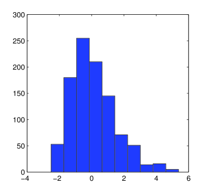
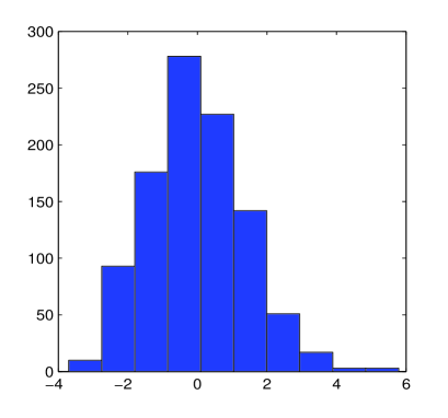
In this section, our first goal is to illustrate Theorem 3.3. We proved that the difference โ€–smโˆ’s^mโ€–22โˆ’pWโ€‹(Sm)superscriptsubscriptnormsubscript๐‘ ๐‘šsubscript^๐‘ ๐‘š22subscript๐‘๐‘Šsubscript๐‘†๐‘š\left\|s_{m}-\hat{s}_{m}\right\|_{2}^{2}-p_{W}(S_{m}) is upper bounded by $\sqrt{d_{m}}/n$, we will show that this bound is sharp on some simulations. Then, we will consider a more general version of Efronโ€™s heuristics, which states that, for a good choice of the constant $C_{W}$, the distribution of โ€–smโˆ’s^mโ€–22superscriptsubscriptnormsubscript๐‘ ๐‘šsubscript^๐‘ ๐‘š22\left\|s_{m}-\hat{s}_{m}\right\|_{2}^{2} is close to the conditional distribution $\mathcal{D}^{W}\left(C_{W}\sum_{\lambda\in\Lambda_{m}}[(P^{W}_{n}-\bar{W}_{n})\psi_{\lambda}]^{2}\right)$. The quantiles of โ€–smโˆ’s^mโ€–22superscriptsubscriptnormsubscript๐‘ ๐‘šsubscript^๐‘ ๐‘š22\left\|s_{m}-\hat{s}_{m}\right\|_{2}^{2} must then be close to their resampled counterpart. In a second simulation, we test this method and remark that it gives very good practical results.

5.1 Illustration of Theorem 3.3

In this simulation, s๐‘ s is the uniform density on $[0,1]$, $S_{m}$ is the set of histograms on the partition $([(k-1)/d_{m},k/d_{m}))_{k=1,...,d_{m}}$. $(W_{1},...,W_{n})$ are Efronโ€™s weights, i.e. the distribution $\mathcal{D}(W_{1},...,W_{n})$ is the multinomial distribution $\mathcal{M}(n,1/n,...,1/n)$. In order to compute $p_{W}(S_{m})$, we estimate the conditional expectation $\mathbb{E}^{W}(\sum_{\lambda\in\Lambda}[(P^{W}_{n}-\bar{W}_{n})\psi_{\lambda}]^{2})$ by a Monte Carlo method with $n_{b}$ repetitions. Finally, we repeat $p=1000$ times the experiment. We plot the histograms of the $p$ values of the normalized difference nโ€‹(โ€–smโˆ’s^mโ€–22โˆ’pWโ€‹(Sm))/dm๐‘›superscriptsubscriptnormsubscript๐‘ ๐‘šsubscript^๐‘ ๐‘š22subscript๐‘๐‘Šsubscript๐‘†๐‘šsubscript๐‘‘๐‘šn(\left\|s_{m}-\hat{s}_{m}\right\|_{2}^{2}-p_{W}(S_{m}))/\sqrt{d_{m}}. The first histogram is obtained with $n=50,d_{m}=10,n_{b}=100$ and the second for $n=200,d_{m}=50,n_{b}=500$.

Refer to caption
Refer to caption
Figure 1: ndmโ€‹(โ€–smโˆ’s^mโ€–22โˆ’pWโ€‹(Sm))๐‘›subscript๐‘‘๐‘šsuperscriptsubscriptnormsubscript๐‘ ๐‘šsubscript^๐‘ ๐‘š22subscript๐‘๐‘Šsubscript๐‘†๐‘š\frac{n}{\sqrt{d_{m}}}(\left\|s_{m}-\hat{s}_{m}\right\|_{2}^{2}-p_{W}(S_{m})).

Comments:

  • โ€ข

    The distribution of nโ€‹(โ€–smโˆ’s^mโ€–22โˆ’pWโ€‹(Sm))/dm๐‘›superscriptsubscriptnormsubscript๐‘ ๐‘šsubscript^๐‘ ๐‘š22subscript๐‘๐‘Šsubscript๐‘†๐‘šsubscript๐‘‘๐‘šn(\left\|s_{m}-\hat{s}_{m}\right\|_{2}^{2}-p_{W}(S_{m}))/\sqrt{d_{m}} does not change with $n$ or $d_{m}$. This shows that the result of Theorem 3.3 is sharp in this example, at least, up to the constant in front of the remainder term.

5.2 Illustration of the second Efronโ€™s heuristic

In this simulation, we keep the same s๐‘ s and the same resampling scheme. $S_{m}$ is the set of functions constant on the partition $([(k-1)/d_{m},k/d_{m}))_{k=1,...,d_{m}}$, with $d_{m}=50$. $n=100$, $N=100$ and $((X_{i}^{J})_{i=1,...,n})_{J=1,...,N}$ are $N$ independent samples with common law โ„™ssubscriptโ„™๐‘ \mathbb{P}_{s}. For all $J=1,...,N$, we compute the projection estimator s^mJsuperscriptsubscript^๐‘ ๐‘š๐ฝ\hat{s}_{m}^{J} on $S_{m}$ with the sample $(X_{i}^{J})_{i=1,...,n}$. Then, we take $n_{b}=10000$ resampling schemes $(W_{1},...,W_{n})$. For all resampling schemes, we compute the quantity

$$p^{J}_{W}(S_{m})=\frac{1}{v_{W}^{2}}\left(\sum_{\lambda\in\Lambda}[(P^{J,W}_{n}-\bar{W}_{n}P_{n}^{J})\psi_{\lambda}]^{2}\right)$$

and we obtain an approximation of the $(1-\alpha)$-quantiles $\hat{q}^{J}_{\alpha}$ of its conditional distribution $\mathcal{D}^{W}(p^{J}_{W}(S_{m}))$. We plot the frequency of $J$ such that โ€–smโˆ’s^mJโ€–2โ‰คq^ฮฑJsuperscriptnormsubscript๐‘ ๐‘šsubscriptsuperscript^๐‘ ๐ฝ๐‘š2subscriptsuperscript^๐‘ž๐ฝ๐›ผ\left\|s_{m}-\hat{s}^{J}_{m}\right\|^{2}\leq\hat{q}^{J}_{\alpha} and the function $f(\alpha)=\alpha$ when $\alpha$ varies in $(0.5,1)$ in the following curves.

[Uncaptioned image]

Comments

  • โ€ข

    The covering property of this empirical ball is very close to the one we would like to obtain. Hence, this method seems to give sharp confidence balls for smsubscript๐‘ ๐‘šs_{m}. The computation time is the same as in the first method.

  • โ€ข

    We do not prove any theoretical evidence of this covering property. In particular, we cannot guarantee that โ„™sโ€‹(โ€–smโˆ’s^mโ€–22โ‰คq^ฮฑ)โ‰ฅ1โˆ’ฮฑsubscriptโ„™๐‘ superscriptsubscriptnormsubscript๐‘ ๐‘šsubscript^๐‘ ๐‘š22subscript^๐‘ž๐›ผ1๐›ผ\mathbb{P}_{s}(\left\|s_{m}-\hat{s}_{m}\right\|_{2}^{2}\leq\hat{q}_{\alpha})\geq 1-\alpha occurs for any $n$.

Acknowledgements: The author would like to thank gratefully Bรฉatrice Laurent and Clรฉmentine Prieur for many fruitful advices.
He also would like to thank the reviewers and the associated editors who helped to improve a first version of the article.

6 Proofs.

6.1 Proof of Theorem 3.3

The theorem can easily be deduced from the following Lemmas, whose proofs are postponed to the appendix.

Lemma 6.1.

Let $X_{1},...,X_{n}$ be an i.i.d sample with common density s๐‘ s in $L^{2}(\mu)$ and let $(\psi_{\lambda})_{\lambda\in\Lambda}$ be an orthonormal system in $L^{2}(\mu)$. Let $W_{1},...W_{n}$ be a resampling scheme, let $\bar{W_{n}}=n^{-1}\sum_{i=1}^{n}W_{i}$ and let $C_{W}=\textrm{Var}(W_{1}-\bar{W_{n}})^{-1}$.
Let Tsโ€‹(ฮ›)=โˆ‘ฮปโˆˆฮ›(ฯˆฮปโˆ’Psโ€‹ฯˆฮป)2subscript๐‘‡๐‘ ฮ›subscript๐œ†ฮ›superscriptsubscript๐œ“๐œ†subscript๐‘ƒ๐‘ subscript๐œ“๐œ†2T_{s}(\Lambda)=\sum_{\lambda\in\Lambda}(\psi_{\lambda}-P_{s}\psi_{\lambda})^{2},

psโ€‹(ฮ›)=โˆ‘ฮปโˆˆฮ›[(Pnโˆ’Ps)โ€‹ฯˆฮป]2,pWโ€‹(ฮ›)=CWโ€‹๐”ผWโ€‹(โˆ‘ฮปโˆˆฮ›[(PnWโˆ’Wnยฏโ€‹Pn)โ€‹ฯˆฮป]2),formulae-sequencesubscript๐‘๐‘ ฮ›subscript๐œ†ฮ›superscriptdelimited-[]subscript๐‘ƒ๐‘›subscript๐‘ƒ๐‘ subscript๐œ“๐œ†2subscript๐‘๐‘Šฮ›subscript๐ถ๐‘Šsubscript๐”ผ๐‘Šsubscript๐œ†ฮ›superscriptdelimited-[]subscriptsuperscript๐‘ƒ๐‘Š๐‘›ยฏsubscript๐‘Š๐‘›subscript๐‘ƒ๐‘›subscript๐œ“๐œ†2p_{s}(\Lambda)=\sum_{\lambda\in\Lambda}\left[(P_{n}-P_{s})\psi_{\lambda}\right]^{2},\;p_{W}(\Lambda)=C_{W}\mathbb{E}_{W}\left(\sum_{\lambda\in\Lambda}\left[(P^{W}_{n}-\bar{W_{n}}P_{n})\psi_{\lambda}\right]^{2}\right),
Usโ€‹(ฮ›)=1nโ€‹(nโˆ’1)โ€‹โˆ‘iโ‰ j=1nโˆ‘ฮปโˆˆฮ›(ฯˆฮปโ€‹(Xi)โˆ’Psโ€‹ฯˆฮป)โ€‹(ฯˆฮปโ€‹(Xj)โˆ’Psโ€‹ฯˆฮป).subscript๐‘ˆ๐‘ ฮ›1๐‘›๐‘›1superscriptsubscript๐‘–๐‘—1๐‘›subscript๐œ†ฮ›subscript๐œ“๐œ†subscript๐‘‹๐‘–subscript๐‘ƒ๐‘ subscript๐œ“๐œ†subscript๐œ“๐œ†subscript๐‘‹๐‘—subscript๐‘ƒ๐‘ subscript๐œ“๐œ†U_{s}(\Lambda)=\frac{1}{n(n-1)}\sum_{i\neq j=1}^{n}\sum_{\lambda\in\Lambda}(\psi_{\lambda}(X_{i})-P_{s}\psi_{\lambda})(\psi_{\lambda}(X_{j})-P_{s}\psi_{\lambda}).

Then

psโ€‹(ฮ›)=1nโ€‹Pnโ€‹Tsโ€‹(ฮ›)+nโˆ’1nโ€‹Usโ€‹(ฮ›),pWโ€‹(ฮ›)=1nโ€‹Pnโ€‹Tsโ€‹(ฮ›)โˆ’1nโ€‹Usโ€‹(ฮ›),psโ€‹(ฮ›)โˆ’pWโ€‹(ฮ›)=Usโ€‹(ฮ›).formulae-sequencesubscript๐‘๐‘ ฮ›1๐‘›subscript๐‘ƒ๐‘›subscript๐‘‡๐‘ ฮ›๐‘›1๐‘›subscript๐‘ˆ๐‘ ฮ›formulae-sequencesubscript๐‘๐‘Šฮ›1๐‘›subscript๐‘ƒ๐‘›subscript๐‘‡๐‘ ฮ›1๐‘›subscript๐‘ˆ๐‘ ฮ›subscript๐‘๐‘ ฮ›subscript๐‘๐‘Šฮ›subscript๐‘ˆ๐‘ ฮ›p_{s}(\Lambda)=\frac{1}{n}P_{n}T_{s}(\Lambda)+\frac{n-1}{n}U_{s}(\Lambda),\;p_{W}(\Lambda)=\frac{1}{n}P_{n}T_{s}(\Lambda)-\frac{1}{n}U_{s}(\Lambda),\;p_{s}(\Lambda)-p_{W}(\Lambda)=U_{s}(\Lambda).
Lemma 6.2.

Let $X_{1},...,X_{n}$ be an i.i.d sample with common density s๐‘ s in $L^{2}(\mu)$ and let $(\psi_{\lambda})_{\lambda\in\Lambda}$ be an orthonormal system in $L^{2}(\mu)$. Let Ds,ฮ›=โˆ‘ฮปโˆˆฮ›Psโ€‹((ฯˆฮปโˆ’Psโ€‹ฯˆฮป)2),subscript๐ท๐‘ ฮ›subscript๐œ†ฮ›subscript๐‘ƒ๐‘ superscriptsubscript๐œ“๐œ†subscript๐‘ƒ๐‘ subscript๐œ“๐œ†2D_{s,\Lambda}=\sum_{\lambda\in\Lambda}P_{s}\left((\psi_{\lambda}-P_{s}\psi_{\lambda})^{2}\right),

Usโ€‹(ฮ›)=1nโ€‹(nโˆ’1)โ€‹โˆ‘iโ‰ j=1nโˆ‘ฮปโˆˆฮ›(ฯˆฮปโ€‹(Xi)โˆ’Psโ€‹ฯˆฮป)โ€‹(ฯˆฮปโ€‹(Xj)โˆ’Psโ€‹ฯˆฮป),subscript๐‘ˆ๐‘ ฮ›1๐‘›๐‘›1superscriptsubscript๐‘–๐‘—1๐‘›subscript๐œ†ฮ›subscript๐œ“๐œ†subscript๐‘‹๐‘–subscript๐‘ƒ๐‘ subscript๐œ“๐œ†subscript๐œ“๐œ†subscript๐‘‹๐‘—subscript๐‘ƒ๐‘ subscript๐œ“๐œ†U_{s}(\Lambda)=\frac{1}{n(n-1)}\sum_{i\neq j=1}^{n}\sum_{\lambda\in\Lambda}(\psi_{\lambda}(X_{i})-P_{s}\psi_{\lambda})(\psi_{\lambda}(X_{j})-P_{s}\psi_{\lambda}),
Bโ€‹(ฮ›)={โˆ‘ฮปโˆˆฮ›aฮปโ€‹ฯˆฮป;โˆ‘ฮปโˆˆฮ›aฮป2โ‰ค1},vs,ฮ›2=suptโˆˆBโ€‹(ฮ›)Psโ€‹((tโˆ’Pโ€‹t)2),bฮ›=suptโˆˆBโ€‹(ฮ›)โ€–tโ€–โˆž.formulae-sequence๐ตฮ›subscript๐œ†ฮ›subscript๐‘Ž๐œ†subscript๐œ“๐œ†subscript๐œ†ฮ›superscriptsubscript๐‘Ž๐œ†21formulae-sequencesuperscriptsubscript๐‘ฃ๐‘ ฮ›2subscriptsupremum๐‘ก๐ตฮ›subscript๐‘ƒ๐‘ superscript๐‘ก๐‘ƒ๐‘ก2subscript๐‘ฮ›subscriptsupremum๐‘ก๐ตฮ›subscriptnorm๐‘กB(\Lambda)=\left\{\sum_{\lambda\in\Lambda}a_{\lambda}\psi_{\lambda};\;\sum_{\lambda\in\Lambda}a_{\lambda}^{2}\leq 1\right\},\;v_{s,\Lambda}^{2}=\sup_{t\in B(\Lambda)}P_{s}\left((t-Pt)^{2}\right),\;b_{\Lambda}=\sup_{t\in B(\Lambda)}\left\|t\right\|_{\infty}.

For all $\xi$ in $\{-1,1\}$, for all $x>0$, we have

โ„™sโ€‹(ฮพโ€‹Usโ€‹(ฮ›)>5.7โ€‹vs,ฮ›โ€‹Ds,ฮ›โ€‹xn+8โ€‹vs,ฮ›2โ€‹xn+384โ€‹2โ€‹vs,ฮ›โ€‹bฮ›โ€‹(xn)3/2+2040โ€‹bฮ›2โ€‹(xn)2)โ‰คeโ€‹eโˆ’x.subscriptโ„™๐‘ ๐œ‰subscript๐‘ˆ๐‘ ฮ›5.7subscript๐‘ฃ๐‘ ฮ›subscript๐ท๐‘ ฮ›๐‘ฅ๐‘›8superscriptsubscript๐‘ฃ๐‘ ฮ›2๐‘ฅ๐‘›3842subscript๐‘ฃ๐‘ ฮ›subscript๐‘ฮ›superscript๐‘ฅ๐‘›322040superscriptsubscript๐‘ฮ›2superscript๐‘ฅ๐‘›2๐‘’superscript๐‘’๐‘ฅ\mathbb{P}_{s}\left(\xi U_{s}(\Lambda)>5.7v_{s,\Lambda}\frac{\sqrt{D_{s,\Lambda}x}}{n}+8v_{s,\Lambda}^{2}\frac{x}{n}+384\sqrt{2}v_{s,\Lambda}b_{\Lambda}\left(\frac{x}{n}\right)^{3/2}+2040b_{\Lambda}^{2}\left(\frac{x}{n}\right)^{2}\right)\leq ee^{-x}.
Lemma 6.3.

Let $S$ be a linear space with finite dimension $d$ satisfying assumption H2. Let s๐‘ s be a density in $L^{2}(\mu)\cap L^{\infty}(\mu)$, let $(\psi_{\lambda})_{\lambda\in\Lambda}$ be an orthonormal basis of $S$. Let

Bโ€‹(ฮ›)={โˆ‘ฮปโˆˆฮ›aฮปโ€‹ฯˆฮป;โˆ‘ฮปโˆˆฮ›aฮป2โ‰ค1},vs,ฮ›2=suptโˆˆBโ€‹(ฮ›)Psโ€‹((tโˆ’Pโ€‹t)2),bฮ›=suptโˆˆBโ€‹(ฮ›)โ€–tโ€–โˆž,formulae-sequence๐ตฮ›subscript๐œ†ฮ›subscript๐‘Ž๐œ†subscript๐œ“๐œ†subscript๐œ†ฮ›superscriptsubscript๐‘Ž๐œ†21formulae-sequencesuperscriptsubscript๐‘ฃ๐‘ ฮ›2subscriptsupremum๐‘ก๐ตฮ›subscript๐‘ƒ๐‘ superscript๐‘ก๐‘ƒ๐‘ก2subscript๐‘ฮ›subscriptsupremum๐‘ก๐ตฮ›subscriptnorm๐‘กB(\Lambda)=\left\{\sum_{\lambda\in\Lambda}a_{\lambda}\psi_{\lambda};\;\sum_{\lambda\in\Lambda}a_{\lambda}^{2}\leq 1\right\},v_{s,\Lambda}^{2}=\sup_{t\in B(\Lambda)}P_{s}\left((t-Pt)^{2}\right),\;b_{\Lambda}=\sup_{t\in B(\Lambda)}\left\|t\right\|_{\infty},
Ds,ฮ›=โˆ‘ฮปโˆˆฮ›Psโ€‹((ฯˆฮปโˆ’Psโ€‹ฯˆฮป)2)=Psโ€‹(suptโˆˆBโ€‹(ฮ›)(tโˆ’Psโ€‹t)2).subscript๐ท๐‘ ฮ›subscript๐œ†ฮ›subscript๐‘ƒ๐‘ superscriptsubscript๐œ“๐œ†subscript๐‘ƒ๐‘ subscript๐œ“๐œ†2subscript๐‘ƒ๐‘ subscriptsupremum๐‘ก๐ตฮ›superscript๐‘กsubscript๐‘ƒ๐‘ ๐‘ก2D_{s,\Lambda}=\sum_{\lambda\in\Lambda}P_{s}\left((\psi_{\lambda}-P_{s}\psi_{\lambda})^{2}\right)=P_{s}\left(\sup_{t\in B(\Lambda)}(t-P_{s}t)^{2}\right).

We have

vs,ฮ›2โ‰คโ€–sโ€–โˆžโˆงC1โ€‹โ€–sโ€–โ€‹d,vs,ฮ›2โ‰คDs,ฮ›โ‰คbฮ›2โ‰คC12โ€‹d.formulae-sequencesuperscriptsubscript๐‘ฃ๐‘ ฮ›2subscriptnorm๐‘ subscript๐ถ1norm๐‘ ๐‘‘superscriptsubscript๐‘ฃ๐‘ ฮ›2subscript๐ท๐‘ ฮ›subscriptsuperscript๐‘2ฮ›superscriptsubscript๐ถ12๐‘‘v_{s,\Lambda}^{2}\leq\left\|s\right\|_{\infty}\wedge C_{1}\left\|s\right\|\sqrt{d},\;v_{s,\Lambda}^{2}\leq D_{s,\Lambda}\leq b^{2}_{\Lambda}\leq C_{1}^{2}d.

Let us now explain briefly the proof of Theorem 3.3. Let $X_{1},...,X_{n}$ be an i.i.d sample with common density s๐‘ s in $L^{2}(\mu)\cap L^{\infty}(\mu)$. Let $(\psi_{\lambda})_{\lambda\in\Lambda_{m}}$ be an orthonormal basis in $S_{m}$. It comes from Lemmas 6.1 and 6.2 that, using the notations of these lemmas, for all $x>0$, there exists an absolute constant $\kappa=2040$ such that, with probability larger than $1-e^{-x+1}$

โ€–smโˆ’s^mโ€–2โ‰คpWโ€‹(Sm)+ฮบโ€‹(vs,ฮ›mโ€‹Ds,ฮ›mโ€‹x4โ€‹n+vs,ฮ›m2โ€‹x4โ€‹n+vs,ฮ›mโ€‹bฮ›mโ€‹(xn)3/2+bฮ›m2โ€‹(xn)2).superscriptnormsubscript๐‘ ๐‘šsubscript^๐‘ ๐‘š2subscript๐‘๐‘Šsubscript๐‘†๐‘š๐œ…subscript๐‘ฃ๐‘ subscriptฮ›๐‘šsubscript๐ท๐‘ subscriptฮ›๐‘š๐‘ฅ4๐‘›superscriptsubscript๐‘ฃ๐‘ subscriptฮ›๐‘š2๐‘ฅ4๐‘›subscript๐‘ฃ๐‘ subscriptฮ›๐‘šsubscript๐‘subscriptฮ›๐‘šsuperscript๐‘ฅ๐‘›32superscriptsubscript๐‘subscriptฮ›๐‘š2superscript๐‘ฅ๐‘›2\|s_{m}-\hat{s}_{m}\|^{2}\leq p_{W}(S_{m})+\kappa\left(v_{s,\Lambda_{m}}\frac{\sqrt{D_{s,\Lambda_{m}}x}}{4n}+v_{s,\Lambda_{m}}^{2}\frac{x}{4n}+v_{s,\Lambda_{m}}b_{\Lambda_{m}}\left(\frac{x}{n}\right)^{3/2}+b_{\Lambda_{m}}^{2}\left(\frac{x}{n}\right)^{2}\right). (14)

Since $x\geq 2$, $\sqrt{x}\leq x$ and $x-1\geq x/2$. We have

2โ€‹vs,ฮ›mโ€‹bฮ›mโ€‹(xn)3/2โ‰คvs,ฮ›m2โ€‹xn+bฮ›m2โ€‹(xn)2,vs,ฮ›m2โ‰คDs,ฮ›m.formulae-sequence2subscript๐‘ฃ๐‘ subscriptฮ›๐‘šsubscript๐‘subscriptฮ›๐‘šsuperscript๐‘ฅ๐‘›32superscriptsubscript๐‘ฃ๐‘ subscriptฮ›๐‘š2๐‘ฅ๐‘›superscriptsubscript๐‘subscriptฮ›๐‘š2superscript๐‘ฅ๐‘›2superscriptsubscript๐‘ฃ๐‘ subscriptฮ›๐‘š2subscript๐ท๐‘ subscriptฮ›๐‘š2v_{s,\Lambda_{m}}b_{\Lambda_{m}}\left(\frac{x}{n}\right)^{3/2}\leq v_{s,\Lambda_{m}}^{2}\frac{x}{n}+b_{\Lambda_{m}}^{2}\left(\frac{x}{n}\right)^{2},\;v_{s,\Lambda_{m}}^{2}\leq D_{s,\Lambda_{m}}.

Hence, from (14), with probability larger than $1-e^{-x/2}$,

โ€–smโˆ’s^mโ€–2โ‰คpWโ€‹(Sm)+ฮบโ€‹(vs,ฮ›mโ€‹Ds,ฮ›mโ€‹xn+32โ€‹bฮ›m2โ€‹(xn)2).superscriptnormsubscript๐‘ ๐‘šsubscript^๐‘ ๐‘š2subscript๐‘๐‘Šsubscript๐‘†๐‘š๐œ…subscript๐‘ฃ๐‘ subscriptฮ›๐‘šsubscript๐ท๐‘ subscriptฮ›๐‘š๐‘ฅ๐‘›32superscriptsubscript๐‘subscriptฮ›๐‘š2superscript๐‘ฅ๐‘›2\|s_{m}-\hat{s}_{m}\|^{2}\leq p_{W}(S_{m})+\kappa\left(v_{s,\Lambda_{m}}\frac{\sqrt{D_{s,\Lambda_{m}}}x}{n}+\frac{3}{2}b_{\Lambda_{m}}^{2}\left(\frac{x}{n}\right)^{2}\right).

Since $\sqrt{d_{m}}x/n\leq C_{3}$, $d_{m}x^{2}/n^{2}\leq C_{3}\sqrt{d_{m}}x/n$, from Lemma 6.3,

vs,ฮ›mโ€‹Ds,ฮ›mโ€‹xn+32โ€‹bฮ›m2โ€‹(xn)2โ‰คC1โ€‹(โ€–sโ€–โˆžโˆงC1โ€‹โ€–sโ€–โ€‹dโˆงC12โ€‹d+32โ€‹C1โ€‹C3)โ€‹dmโ€‹xn.subscript๐‘ฃ๐‘ subscriptฮ›๐‘šsubscript๐ท๐‘ subscriptฮ›๐‘š๐‘ฅ๐‘›32superscriptsubscript๐‘subscriptฮ›๐‘š2superscript๐‘ฅ๐‘›2subscript๐ถ1subscriptnorm๐‘ subscript๐ถ1norm๐‘ ๐‘‘superscriptsubscript๐ถ12๐‘‘32subscript๐ถ1subscript๐ถ3subscript๐‘‘๐‘š๐‘ฅ๐‘›v_{s,\Lambda_{m}}\frac{\sqrt{D_{s,\Lambda_{m}}}x}{n}+\frac{3}{2}b_{\Lambda_{m}}^{2}\left(\frac{x}{n}\right)^{2}\leq C_{1}\left(\sqrt{\left\|s\right\|_{\infty}\wedge C_{1}\left\|s\right\|\sqrt{d}\wedge C_{1}^{2}d}+\frac{3}{2}C_{1}C_{3}\right)\frac{\sqrt{d_{m}}x}{n}. (15)

This concludes the proof of Theorem 3.3, with $\kappa_{v}=2040C_{1}(1\vee C_{1}\vee 3C_{1}C_{3}/2)$.

6.2 Proof of Corollary 3.4

We use a union bound to obtain that

โ„™sโ€‹(โˆƒmโˆˆโ„ณn,โ€–smโˆ’s^mโ€–2>Vโ€‹(m,ฮฒ,X1,โ€ฆ,Xn))subscriptโ„™๐‘ formulae-sequence๐‘šsubscriptโ„ณ๐‘›superscriptnormsubscript๐‘ ๐‘šsubscript^๐‘ ๐‘š2๐‘‰๐‘š๐›ฝsubscript๐‘‹1โ€ฆsubscript๐‘‹๐‘›\displaystyle\mathbb{P}_{s}\left(\exists m\in\mathcal{M}_{n},\;\|s_{m}-\hat{s}_{m}\|^{2}>V(m,\beta,X_{1},...,X_{n})\right)
โ‰คNnโ€‹maxmโˆˆโ„ณnโกโ„™sโ€‹(โ€–smโˆ’s^mโ€–2>Vโ€‹(m,ฮฒ,X1,โ€ฆ,Xn)).absentsubscript๐‘๐‘›subscript๐‘šsubscriptโ„ณ๐‘›subscriptโ„™๐‘ superscriptnormsubscript๐‘ ๐‘šsubscript^๐‘ ๐‘š2๐‘‰๐‘š๐›ฝsubscript๐‘‹1โ€ฆsubscript๐‘‹๐‘›\displaystyle\leq N_{n}\max_{m\in\mathcal{M}_{n}}\mathbb{P}_{s}\left(\|s_{m}-\hat{s}_{m}\|^{2}>V(m,\beta,X_{1},...,X_{n})\right).

All the models satisfy H2. From assumption H3$(\mathcal{M},\beta)$, $x_{n}$ satisfies $2\leq x_{n}\leq C_{3}n/\sqrt{d_{m}}$ with $C_{3}=C_{\mathcal{M}}$, thus, from Theorem 3.3, for all $m$ in $\mathcal{M}_{n}$,

โ„™sโ€‹(โ€–smโˆ’s^mโ€–2>Vโ€‹(m,ฮฒ,X1,โ€ฆ,Xn))โ‰คeโˆ’xn/2.subscriptโ„™๐‘ superscriptnormsubscript๐‘ ๐‘šsubscript^๐‘ ๐‘š2๐‘‰๐‘š๐›ฝsubscript๐‘‹1โ€ฆsubscript๐‘‹๐‘›superscript๐‘’subscript๐‘ฅ๐‘›2\mathbb{P}_{s}\left(\|s_{m}-\hat{s}_{m}\|^{2}>V(m,\beta,X_{1},...,X_{n})\right)\leq e^{-x_{n}/2}.

Finally, ${\rm Card}(\mathcal{M}_{n})e^{-x_{n}/2}\leq\frac{\beta}{2}$, which concludes the proof of Corollary 3.4.

6.3 Proof of Theorem 3.5

Let s๐‘ s be a density in $L^{2}(\mu)\cap L^{\infty}(\mu)$, we only have to prove that there exists a constant $\kappa$ such that, with โ„™ssubscriptโ„™๐‘ \mathbb{P}_{s}-probability larger than $1-\alpha$,

โˆ€mโˆˆโ„ณn,pWโ€‹(Sm)โ‰คฮบโ€‹(dmn+(1+โ€–sโ€–โˆžโˆงโ€–sโ€–โ€‹dm1/2โˆงdm)โ€‹dmnโ€‹lnโก[Nnฮฑ]).formulae-sequencefor-all๐‘šsubscriptโ„ณ๐‘›subscript๐‘๐‘Šsubscript๐‘†๐‘š๐œ…subscript๐‘‘๐‘š๐‘›1subscriptnorm๐‘ norm๐‘ superscriptsubscript๐‘‘๐‘š12subscript๐‘‘๐‘šsubscript๐‘‘๐‘š๐‘›subscript๐‘๐‘›๐›ผ\forall m\in\mathcal{M}_{n},\;p_{W}(S_{m})\leq\kappa\left(\frac{d_{m}}{n}+\left(1+\sqrt{\left\|s\right\|_{\infty}\wedge\|s\|d_{m}^{1/2}\wedge d_{m}}\right)\frac{\sqrt{d_{m}}}{n}\ln\left[\frac{N_{n}}{\alpha}\right]\right).

Let $(\psi_{\lambda})_{\lambda\in\Lambda_{m}}$ be an orthonormal basis of $S_{m}$, from Lemma 6.1 and using the notations of this lemma,

pWโ€‹(ฮ›)=1nโ€‹Pnโ€‹Tsโ€‹(ฮ›m)โˆ’1nโ€‹Usโ€‹(ฮ›m).subscript๐‘๐‘Šฮ›1๐‘›subscript๐‘ƒ๐‘›subscript๐‘‡๐‘ subscriptฮ›๐‘š1๐‘›subscript๐‘ˆ๐‘ subscriptฮ›๐‘šp_{W}(\Lambda)=\frac{1}{n}P_{n}T_{s}(\Lambda_{m})-\frac{1}{n}U_{s}(\Lambda_{m}).

We follow the proof of Theorem 3.3. From Lemmas 6.2 and 6.3 and assumptions H1, H2, H3$(\mathcal{M},\alpha)$, there exists a constant $\kappa$ such that

โ„™sโ€‹(โˆƒmโˆˆโ„ณn,Usโ€‹(ฮ›m)>ฮบโ€‹โ€–sโ€–โˆžโˆงโ€–sโ€–โ€‹dm1/2โˆงdmโ€‹dmโ€‹lnโก[Nn/ฮฑ]n)โ‰คฮฑ.subscriptโ„™๐‘ formulae-sequence๐‘šsubscriptโ„ณ๐‘›subscript๐‘ˆ๐‘ subscriptฮ›๐‘š๐œ…subscriptnorm๐‘ norm๐‘ superscriptsubscript๐‘‘๐‘š12subscript๐‘‘๐‘šsubscript๐‘‘๐‘šsubscript๐‘๐‘›๐›ผ๐‘›๐›ผ\mathbb{P}_{s}\left(\exists m\in\mathcal{M}_{n},\;U_{s}(\Lambda_{m})>\kappa\sqrt{\left\|s\right\|_{\infty}\wedge\|s\|d_{m}^{1/2}\wedge d_{m}}\frac{\sqrt{d_{m}}\ln[N_{n}/\alpha]}{n}\right)\leq\alpha.

Moreover, it is easy to check, with Cauchy-Schwarz inequality, that, using the notations of Lemma 6.3

Tsโ€‹(ฮ›m)=suptโˆˆBโ€‹(ฮ›m)(tโˆ’Psโ€‹t)2.subscript๐‘‡๐‘ subscriptฮ›๐‘šsubscriptsupremum๐‘ก๐ตsubscriptฮ›๐‘šsuperscript๐‘กsubscript๐‘ƒ๐‘ ๐‘ก2T_{s}(\Lambda_{m})=\sup_{t\in B(\Lambda_{m})}(t-P_{s}t)^{2}.

Hence, using assumptions H2, we obtain

Pnโ€‹Tsโ€‹(ฮ›m)โ‰คโ€–Tsโ€‹(ฮ›m)โ€–โˆžโ‰ค2โ€‹C12โ€‹dm.subscript๐‘ƒ๐‘›subscript๐‘‡๐‘ subscriptฮ›๐‘šsubscriptnormsubscript๐‘‡๐‘ subscriptฮ›๐‘š2superscriptsubscript๐ถ12subscript๐‘‘๐‘šP_{n}T_{s}(\Lambda_{m})\leq\left\|T_{s}(\Lambda_{m})\right\|_{\infty}\leq 2C_{1}^{2}d_{m}.

This conclude the proof of Theorem 3.5.

6.4 Proof of Lemma 3.7

Let $X_{1},...,X_{n}$ be an i.i.d sample with common density s๐‘ s in $L^{2}(\mu)\cap L^{\infty}(\mu)$. Let $(\psi_{\lambda})_{\lambda\in\Lambda_{n}}$ be an orthonormal basis of $S_{n}$ such that $(\psi_{\lambda})_{\lambda\in\Lambda_{m}}$ is an orthonormal basis of $S_{m}$, with $\Lambda_{m}\subset\Lambda_{n}$. The Hoeffdingโ€™s decomposition of the $U$-statistic $p_{b}(S_{m},S_{n})$ can be written

$\displaystyle p_{b}(S_{m},S_{n})$ $\displaystyle=$ Usโ€‹(ฮ›nโˆ’ฮ›m)+2โ€‹Pnโ€‹(โˆ‘ฮปโˆˆฮ›nโˆ’ฮ›m(Psโ€‹ฯˆฮป)โ€‹(ฯˆฮปโˆ’Psโ€‹ฯˆฮป))+โˆ‘ฮปโˆˆฮ›nโˆ’ฮ›m(Psโ€‹ฯˆฮป)2subscript๐‘ˆ๐‘ subscriptฮ›๐‘›subscriptฮ›๐‘š2subscript๐‘ƒ๐‘›subscript๐œ†subscriptฮ›๐‘›subscriptฮ›๐‘šsubscript๐‘ƒ๐‘ subscript๐œ“๐œ†subscript๐œ“๐œ†subscript๐‘ƒ๐‘ subscript๐œ“๐œ†subscript๐œ†subscriptฮ›๐‘›subscriptฮ›๐‘šsuperscriptsubscript๐‘ƒ๐‘ subscript๐œ“๐œ†2\displaystyle U_{s}(\Lambda_{n}-\Lambda_{m})+2P_{n}\left(\sum_{\lambda\in\Lambda_{n}-\Lambda_{m}}(P_{s}\psi_{\lambda})(\psi_{\lambda}-P_{s}\psi_{\lambda})\right)+\sum_{\lambda\in\Lambda_{n}-\Lambda_{m}}(P_{s}\psi_{\lambda})^{2}
$\displaystyle=$ Usโ€‹(ฮ›nโˆ’ฮ›m)+2โ€‹(Pnโˆ’Ps)โ€‹(snโˆ’sm)+โ€–snโˆ’smโ€–2,subscript๐‘ˆ๐‘ subscriptฮ›๐‘›subscriptฮ›๐‘š2subscript๐‘ƒ๐‘›subscript๐‘ƒ๐‘ subscript๐‘ ๐‘›subscript๐‘ ๐‘šsuperscriptnormsubscript๐‘ ๐‘›subscript๐‘ ๐‘š2\displaystyle U_{s}(\Lambda_{n}-\Lambda_{m})+2(P_{n}-P_{s})\left(s_{n}-s_{m}\right)+\|s_{n}-s_{m}\|^{2},

where, as usually, for all indexes sets $\Lambda$,

Usโ€‹(ฮ›)=1nโ€‹(nโˆ’1)โ€‹โˆ‘iโ‰ j=1nโˆ‘ฮปโˆˆฮ›(ฯˆฮปโ€‹(Xi)โˆ’Psโ€‹ฯˆฮป)โ€‹(ฯˆฮปโ€‹(Xj)โˆ’Psโ€‹ฯˆฮป).subscript๐‘ˆ๐‘ ฮ›1๐‘›๐‘›1superscriptsubscript๐‘–๐‘—1๐‘›subscript๐œ†ฮ›subscript๐œ“๐œ†subscript๐‘‹๐‘–subscript๐‘ƒ๐‘ subscript๐œ“๐œ†subscript๐œ“๐œ†subscript๐‘‹๐‘—subscript๐‘ƒ๐‘ subscript๐œ“๐œ†U_{s}(\Lambda)=\frac{1}{n(n-1)}\sum_{i\neq j=1}^{n}\sum_{\lambda\in\Lambda}(\psi_{\lambda}(X_{i})-P_{s}\psi_{\lambda})(\psi_{\lambda}(X_{j})-P_{s}\psi_{\lambda}).

It comes from Lemmas 6.2 and 6.3 that, for all $2\leq x\leq C_{3}n/\sqrt{d_{n}}$,

โ„™sโ€‹(|Usโ€‹(ฮ›nโˆ’ฮ›m)|>ฮบvโ€‹(C1,C3)โ€‹(1+โ€–sโ€–โˆžโˆงโ€–sโ€–โ€‹dn1/2)โ€‹dnโ€‹xn)โ‰ค2โ€‹eโˆ’x/2.subscriptโ„™๐‘ subscript๐‘ˆ๐‘ subscriptฮ›๐‘›subscriptฮ›๐‘šsubscript๐œ…๐‘ฃsubscript๐ถ1subscript๐ถ31subscriptnorm๐‘ norm๐‘ superscriptsubscript๐‘‘๐‘›12subscript๐‘‘๐‘›๐‘ฅ๐‘›2superscript๐‘’๐‘ฅ2\mathbb{P}_{s}\left(|U_{s}(\Lambda_{n}-\Lambda_{m})|>\kappa_{v}(C_{1},C_{3})\left(1+\sqrt{\left\|s\right\|_{\infty}\wedge\left\|s\right\|d_{n}^{1/2}}\right)\frac{\sqrt{d_{n}}x}{n}\right)\leq 2e^{-x/2}.

If sn=smsubscript๐‘ ๐‘›subscript๐‘ ๐‘šs_{n}=s_{m}, this concludes the proof. Else, let $\epsilon$ in $(0,1)$, the inequality $2ab\leq\epsilon a^{2}+\epsilon^{-1}b^{2}$ gives

2โ€‹|(Pnโˆ’Ps)โ€‹(snโˆ’sm)|โ‰คฯตโ€‹โ€–snโˆ’smโ€–2+ฯตโˆ’1โ€‹((Pnโˆ’Ps)โ€‹(snโˆ’smโ€–snโˆ’smโ€–))2.2subscript๐‘ƒ๐‘›subscript๐‘ƒ๐‘ subscript๐‘ ๐‘›subscript๐‘ ๐‘šitalic-ฯตsuperscriptnormsubscript๐‘ ๐‘›subscript๐‘ ๐‘š2superscriptitalic-ฯต1superscriptsubscript๐‘ƒ๐‘›subscript๐‘ƒ๐‘ subscript๐‘ ๐‘›subscript๐‘ ๐‘šnormsubscript๐‘ ๐‘›subscript๐‘ ๐‘š22|(P_{n}-P_{s})\left(s_{n}-s_{m}\right)|\leq\epsilon\|s_{n}-s_{m}\|^{2}+\epsilon^{-1}\left((P_{n}-P_{s})\left(\frac{s_{n}-s_{m}}{\|s_{n}-s_{m}\|}\right)\right)^{2}.

The function sm,n=(snโˆ’sm)/โ€–snโˆ’smโ€–subscript๐‘ ๐‘š๐‘›subscript๐‘ ๐‘›subscript๐‘ ๐‘šnormsubscript๐‘ ๐‘›subscript๐‘ ๐‘šs_{m,n}=(s_{n}-s_{m})/\|s_{n}-s_{m}\| satisfies โ€–sm,nโ€–โ‰ค1normsubscript๐‘ ๐‘š๐‘›1\|s_{m,n}\|\leq 1 and, from Bernsteinโ€™s inequality, for all $x>0$,

โ„™sโ€‹(|(Pnโˆ’Ps)โ€‹(sn,m)|>2โ€‹Psโ€‹[(sm,nโˆ’Psโ€‹sm,n)2]โ€‹xn+โ€–sn,mโ€–โˆžโ€‹x3โ€‹n)โ‰ค2โ€‹eโˆ’x.subscriptโ„™๐‘ subscript๐‘ƒ๐‘›subscript๐‘ƒ๐‘ subscript๐‘ ๐‘›๐‘š2subscript๐‘ƒ๐‘ delimited-[]superscriptsubscript๐‘ ๐‘š๐‘›subscript๐‘ƒ๐‘ subscript๐‘ ๐‘š๐‘›2๐‘ฅ๐‘›subscriptnormsubscript๐‘ ๐‘›๐‘š๐‘ฅ3๐‘›2superscript๐‘’๐‘ฅ\mathbb{P}_{s}\left(|(P_{n}-P_{s})\left(s_{n,m}\right)|>\sqrt{2P_{s}\left[(s_{m,n}-P_{s}s_{m,n})^{2}\right]\frac{x}{n}}+\left\|s_{n,m}\right\|_{\infty}\frac{x}{3n}\right)\leq 2e^{-x}.

Since sm,nsubscript๐‘ ๐‘š๐‘›s_{m,n} belongs to $S_{n}$, which satisfies H2, it comes from Lemma 6.3 that

Psโ€‹[(sm,nโˆ’Psโ€‹sm,n)2]โ‰ค(โ€–sโ€–โˆžโˆงC1โ€‹โ€–sโ€–โ€‹dn1/2),โ€–sn,mโ€–โˆžโ‰คC1โ€‹dn.formulae-sequencesubscript๐‘ƒ๐‘ delimited-[]superscriptsubscript๐‘ ๐‘š๐‘›subscript๐‘ƒ๐‘ subscript๐‘ ๐‘š๐‘›2subscriptnorm๐‘ subscript๐ถ1norm๐‘ superscriptsubscript๐‘‘๐‘›12subscriptnormsubscript๐‘ ๐‘›๐‘šsubscript๐ถ1subscript๐‘‘๐‘›P_{s}\left[(s_{m,n}-P_{s}s_{m,n})^{2}\right]\leq\left(\left\|s\right\|_{\infty}\wedge C_{1}\left\|s\right\|d_{n}^{1/2}\right),\;\left\|s_{n,m}\right\|_{\infty}\leq C_{1}\sqrt{d_{n}}.

We conclude the proof of Lemma 3.7 saying that $x\geq 2$ implies $2e^{-x}\leq e^{-x/2}$. In this Lemma, we proved that we can choose $\kappa_{b}(\epsilon,C_{3})=\kappa_{v}(C_{1},C_{3})+2\epsilon^{-1}(2\vee 2C_{1}\vee C_{3}C_{1}^{2}/9).$

6.5 Proof of Corollary 3.8

Let $X_{1},...,X_{n}$ be an iid sample with common density s๐‘ s in $B_{2,\infty}(M_{2},M_{\infty},0,L^{2}(\mu))$. Let $\epsilon$ in $(0,1)$ and let $\Omega_{n}(\epsilon)$ denote the event

$\displaystyle\left\{\vphantom{\frac{\sqrt{d_{n}}x_{n}}{n}}\forall m\in\mathcal{M}_{n},\;\left|p_{b}(S_{m},S_{n})-\|s_{n}-s_{m}\|^{2}\right|\leq\right.$ ฯตโ€‹โ€–snโˆ’smโ€–2italic-ฯตsuperscriptnormsubscript๐‘ ๐‘›subscript๐‘ ๐‘š2\displaystyle\left.\epsilon\|s_{n}-s_{m}\|^{2}\right.
$\displaystyle\left.+\kappa_{b}(\epsilon,C_{\mathcal{M}})\sqrt{\left\|s\right\|_{\infty}\wedge\left\|s\right\|d_{n}^{1/2}}\frac{\sqrt{d_{n}}x_{n}}{n}\right\}.$

A union bound gives that โ„™sโ€‹(ฮฉnโ€‹(ฯต)c)subscriptโ„™๐‘ subscriptฮฉ๐‘›superscriptitalic-ฯต๐‘\mathbb{P}_{s}(\Omega_{n}(\epsilon)^{c}) is upper bounded by the sum over $\mathcal{M}_{n}$ of

โ„™sโ€‹(|pbโ€‹(Sm,Sn)โˆ’โ€–snโˆ’smโ€–2|>ฯตโ€‹โ€–snโˆ’smโ€–2+ฮบbโ€‹(ฯต,Cโ„ณ)โ€‹โ€–sโ€–โˆžโˆงโ€–sโ€–โ€‹dn1/2โ€‹dnโ€‹xnn).subscriptโ„™๐‘ subscript๐‘๐‘subscript๐‘†๐‘šsubscript๐‘†๐‘›superscriptnormsubscript๐‘ ๐‘›subscript๐‘ ๐‘š2italic-ฯตsuperscriptnormsubscript๐‘ ๐‘›subscript๐‘ ๐‘š2subscript๐œ…๐‘italic-ฯตsubscript๐ถโ„ณsubscriptnorm๐‘ norm๐‘ superscriptsubscript๐‘‘๐‘›12subscript๐‘‘๐‘›subscript๐‘ฅ๐‘›๐‘›\mathbb{P}_{s}\left(\left|p_{b}(S_{m},S_{n})-\|s_{n}-s_{m}\|^{2}\right|>\epsilon\|s_{n}-s_{m}\|^{2}+\kappa_{b}(\epsilon,C_{\mathcal{M}})\sqrt{\left\|s\right\|_{\infty}\wedge\left\|s\right\|d_{n}^{1/2}}\frac{\sqrt{d_{n}}x_{n}}{n}\right).

Assumption H3$(\mathcal{M},\beta)$ ensures that $x_{n}$ satisfies $2\leq x_{n}\leq C_{3}n/\sqrt{d_{m}}$ with $C_{3}=C_{\mathcal{M}}$, thus, Lemma 3.7 gives that this last probability is upper bounded by $3e^{-x_{n}/2}$. Our choice of $x_{n}$ ensures that $3N_{n}e^{-x_{n}/2}\leq\beta/2$ and thus that โ„™sโ€‹(ฮฉnโ€‹(ฯต)c)โ‰คฮฒ2.subscriptโ„™๐‘ subscriptฮฉ๐‘›superscriptitalic-ฯต๐‘๐›ฝ2\mathbb{P}_{s}(\Omega_{n}(\epsilon)^{c})\leq\frac{\beta}{2}. The proof of Corollary 3.8 is concluded because, on $\Omega_{n}(\epsilon)$,

(1โˆ’ฯต)โ€‹โ€–snโˆ’smโ€–2โ‰คpbโ€‹(Sm,Sn)+ฮบbโ€‹(ฯต,Cโ„ณ)โ€‹โ€–sโ€–โˆžโˆงโ€–sโ€–โ€‹dn1/2โ€‹dnโ€‹xnn.1italic-ฯตsuperscriptnormsubscript๐‘ ๐‘›subscript๐‘ ๐‘š2subscript๐‘๐‘subscript๐‘†๐‘šsubscript๐‘†๐‘›subscript๐œ…๐‘italic-ฯตsubscript๐ถโ„ณsubscriptnorm๐‘ norm๐‘ superscriptsubscript๐‘‘๐‘›12subscript๐‘‘๐‘›subscript๐‘ฅ๐‘›๐‘›(1-\epsilon)\|s_{n}-s_{m}\|^{2}\leq p_{b}(S_{m},S_{n})+\kappa_{b}(\epsilon,C_{\mathcal{M}})\sqrt{\left\|s\right\|_{\infty}\wedge\left\|s\right\|d_{n}^{1/2}}\frac{\sqrt{d_{n}}x_{n}}{n}.

6.6 Proof of Theorem 4.1

The theorem is a straightforward consequence of Corollaries 3.4 and 3.8.

6.7 Proof of Theorem 4.2

We begin the proof with the following proposition, which shows that $\phi_{n}(\alpha,\beta,S_{m},S_{m})\geq d_{m}/(12n)$. Since $\phi_{n}(\alpha,\beta,S_{n},S_{m})\geq\phi_{n}(\alpha,\beta,S_{m},S_{m})$, the same bound holds also for $\phi_{n}(\alpha,\beta,S_{n},S_{m})$.

Proposition 6.4.

Let $S$ be the set of histograms on the partition,

$$\left\{\left[\frac{k}{d},\frac{k+1}{d}\right),\;k=0,...,d-1\right\}.$$

Let $X_{1},...,X_{n}$ be an i.i.d sample. Let $\alpha,\beta$ be real numbers in $(0,1)$ such that $\alpha+\beta<1$. Assume that $d\geq 3+18\log(\sqrt{2}/(1-\alpha-\beta))$, then

$$\phi_{n}(\alpha,\beta,S,S)\geq\frac{d}{12n}.$$

The proof is decomposed in two lemmas.

Lemma 6.5.

Let B^ฮฒ=B2โ€‹(s^,ฯ^ฮฒ,S)subscript^๐ต๐›ฝsubscript๐ต2^๐‘ subscript^๐œŒ๐›ฝ๐‘†\hat{B}_{\beta}=B_{2}(\hat{s},\hat{\rho}_{\beta},S) in $CS(S,\beta)$ and let $\rho_{\alpha,\beta}$ be a real number such that

โˆ€sโˆˆS,โ„™sโ€‹(ฯ^ฮฒโ‰คฯฮฑ,ฮฒ)โ‰ฅ1โˆ’ฮฑ.formulae-sequencefor-all๐‘ ๐‘†subscriptโ„™๐‘ subscript^๐œŒ๐›ฝsubscript๐œŒ๐›ผ๐›ฝ1๐›ผ\forall s\in S,\;\mathbb{P}_{s}\left(\hat{\rho}_{\beta}\leq\rho_{\alpha,\beta}\right)\geq 1-\alpha.

Then,

โˆ€sโˆˆS,โ„™sโ€‹(โ€–sโˆ’s^โ€–>ฯฮฑ,ฮฒ)โ‰คฮฑ+ฮฒ.formulae-sequencefor-all๐‘ ๐‘†subscriptโ„™๐‘ norm๐‘ ^๐‘ subscript๐œŒ๐›ผ๐›ฝ๐›ผ๐›ฝ\forall s\in S,\;\mathbb{P}_{s}\left(\left\|s-\hat{s}\right\|>\rho_{\alpha,\beta}\right)\leq\alpha+\beta. (16)
Proof.

of Lemma 6.5:

โ„™sโ€‹[โ€–sโˆ’s^โ€–>ฯฮฑ,ฮฒ]subscriptโ„™๐‘ delimited-[]norm๐‘ ^๐‘ subscript๐œŒ๐›ผ๐›ฝ\displaystyle\mathbb{P}_{s}\left[\left\|s-\hat{s}\right\|>\rho_{\alpha,\beta}\right] $\displaystyle=$ โ„™sโ€‹[โ€–sโˆ’s^โ€–>ฯฮฑ,ฮฒโˆฉฯฮฑ,ฮฒโ‰ฅฯ^ฮฒ]subscriptโ„™๐‘ delimited-[]norm๐‘ ^๐‘ subscript๐œŒ๐›ผ๐›ฝsubscript๐œŒ๐›ผ๐›ฝsubscript^๐œŒ๐›ฝ\displaystyle\mathbb{P}_{s}\left[\left\|s-\hat{s}\right\|>\rho_{\alpha,\beta}\cap\rho_{\alpha,\beta}\geq\hat{\rho}_{\beta}\right]
+โ„™sโ€‹[โ€–sโˆ’s^โ€–>ฯฮฑ,ฮฒโˆฉฯฮฑ,ฮฒ<ฯ^ฮฒ]subscriptโ„™๐‘ delimited-[]norm๐‘ ^๐‘ subscript๐œŒ๐›ผ๐›ฝsubscript๐œŒ๐›ผ๐›ฝsubscript^๐œŒ๐›ฝ\displaystyle+\mathbb{P}_{s}\left[\left\|s-\hat{s}\right\|>\rho_{\alpha,\beta}\cap\rho_{\alpha,\beta}<\hat{\rho}_{\beta}\right]
$\displaystyle\leq$ โ„™sโ€‹[โ€–sโˆ’s^โ€–>ฯ^ฮฒ]+โ„™sโ€‹[ฯฮฑ,ฮฒ<ฯ^ฮฒ]โ‰คฮฑ+ฮฒ.subscriptโ„™๐‘ delimited-[]norm๐‘ ^๐‘ subscript^๐œŒ๐›ฝsubscriptโ„™๐‘ delimited-[]subscript๐œŒ๐›ผ๐›ฝsubscript^๐œŒ๐›ฝ๐›ผ๐›ฝ\displaystyle\mathbb{P}_{s}\left[\left\|s-\hat{s}\right\|>\hat{\rho}_{\beta}\right]+\mathbb{P}_{s}\left[\rho_{\alpha,\beta}<\hat{\rho}_{\beta}\right]\leq\alpha+\beta.

โˆŽ

Lemma 6.6.

Let $\delta=\alpha+\beta$ and let $\rho_{\delta}$ be any real number satisfying (16). Then we have

$$\rho_{\delta}^{2}\geq\frac{d-1}{2n}-\frac{1}{n}\sqrt{2(d+1)\ln\left[\frac{\sqrt{1+(d+1)n^{-1}}}{1-\delta}\right]}.$$

Remark: When $d\geq 3+18\log(\sqrt{2}/(1-\delta))$ and $n\geq d+1$, we have

$$\sqrt{2(d+1)\ln\left[\frac{\sqrt{1+(d+1)n^{-1}}}{1-\delta}\right]}\leq\frac{d-1}{3},$$

thus $\rho_{\delta}^{2}\geq(d-1)/(6n)\geq d/(12n)$.

Proof: We prove that if

$$\rho_{\delta}^{2}=\frac{d-1}{2n}-\frac{1}{n}\sqrt{2(d+1)\ln\left[\frac{\sqrt{1+(d+1)n^{-1}}}{1-\delta}\right]}$$

then

infsโˆˆSโ„™sโ€‹[โ€–sโˆ’s^โ€–โ‰คฯฮด]โ‰ค1โˆ’ฮด.subscriptinfimum๐‘ ๐‘†subscriptโ„™๐‘ delimited-[]norm๐‘ ^๐‘ subscript๐œŒ๐›ฟ1๐›ฟ\inf_{s\in S}\mathbb{P}_{s}\left[\left\|s-\hat{s}\right\|\leq\rho_{\delta}\right]\leq 1-\delta.

Let s0=1[0,1)subscript๐‘ 0subscript101s_{0}=1_{[0,1)}, $\Lambda=\{1,...,[d/2]\}$ and for all $\lambda$ in $\Lambda$, let

$$\psi_{\lambda}=\sqrt{\frac{d}{2}}\left(1_{[2(\lambda-1)/d,(2\lambda-1)/d)}-1_{[(2\lambda-1)/d,2\lambda/d)}\right).$$

It is easy to check that $(\psi_{\lambda})_{\lambda\in\Lambda}$ is an orthonormal system in $S$, orthogonal to s0subscript๐‘ 0s_{0} such that, for all $\lambda$ in $\Lambda$, $\left\|\psi_{\lambda}\right\|_{\infty}\leq\sqrt{d/2}$. Let s^0=โˆซs^โ€‹s0โ€‹๐‘‘ฮผsubscript^๐‘ 0^๐‘ subscript๐‘ 0differential-d๐œ‡\hat{s}_{0}=\int\hat{s}s_{0}d\mu and for all $\lambda$ in $\Lambda$, let

s^ฮป=โˆซs^โ€‹ฯˆฮปโ€‹๐‘‘ฮผ.subscript^๐‘ ๐œ†^๐‘ subscript๐œ“๐œ†differential-d๐œ‡\hat{s}_{\lambda}=\int\hat{s}\psi_{\lambda}d\mu.

Let $(\xi_{\lambda})_{\lambda\in\Lambda}$ be independent Rademacher random variables, independent of $X_{1},...,X_{n}$, let $\rho$ be some real number to be chosen later and let sฮพ=s0+ฯโ€‹โˆ‘ฮปโˆˆฮ›ฮพฮปโ€‹ฯˆฮป.subscript๐‘ ๐œ‰subscript๐‘ 0๐œŒsubscript๐œ†ฮ›subscript๐œ‰๐œ†subscript๐œ“๐œ†s_{\xi}=s_{0}+\rho\sum_{\lambda\in\Lambda}\xi_{\lambda}\psi_{\lambda}. The $\psi_{\lambda}$ have distinct support, thus $\left\|\sum_{\lambda\in\Lambda}|\psi_{\lambda}|\right\|_{\infty}\leq\sqrt{d/2}$ and sฮพsubscript๐‘ ๐œ‰s_{\xi} is a density if

$$-\sqrt{\frac{2}{d}}\leq\rho\leq\sqrt{\frac{2}{d}}$$ (17)

Assume that (17) holds, then

infsโˆˆSโ„™sโ€‹[โ€–sโˆ’s^โ€–โ‰คฯฮด]subscriptinfimum๐‘ ๐‘†subscriptโ„™๐‘ delimited-[]norm๐‘ ^๐‘ subscript๐œŒ๐›ฟ\displaystyle\inf_{s\in S}\mathbb{P}_{s}\left[\left\|s-\hat{s}\right\|\leq\rho_{\delta}\right] $\displaystyle\leq$ โ„™sฮพโ€‹[โ€–sฮพโˆ’s^โ€–โ‰คฯฮด].subscriptโ„™subscript๐‘ ๐œ‰delimited-[]normsubscript๐‘ ๐œ‰^๐‘ subscript๐œŒ๐›ฟ\displaystyle\mathbb{P}_{s_{\xi}}\left[\left\|s_{\xi}-\hat{s}\right\|\leq\rho_{\delta}\right]. (18)

We have

โ€–sฮพโˆ’s^โ€–2superscriptnormsubscript๐‘ ๐œ‰^๐‘ 2\displaystyle\left\|s_{\xi}-\hat{s}\right\|^{2} $\displaystyle=$ (1+s0)2+โˆ‘ฮปโˆˆฮ›(ฯโ€‹ฮพฮปโˆ’s^ฮป)2superscript1subscript๐‘ 02subscript๐œ†ฮ›superscript๐œŒsubscript๐œ‰๐œ†subscript^๐‘ ๐œ†2\displaystyle(1+s_{0})^{2}+\sum_{\lambda\in\Lambda}\left(\rho\xi_{\lambda}-\hat{s}_{\lambda}\right)^{2} (19)
$\displaystyle=$ โˆ‘ฮปโˆˆฮ›,ฯโ€‹ฮพฮปโ€‹s^ฮปโ‰ค0ฯ2โˆ’2โ€‹ฯโ€‹ฮพฮปโ€‹s^ฮป+s^ฮป2โ‰ฅฯ2โ€‹Nโ€‹(ฮพ,s^),subscriptformulae-sequence๐œ†ฮ›๐œŒsubscript๐œ‰๐œ†subscript^๐‘ ๐œ†0superscript๐œŒ22๐œŒsubscript๐œ‰๐œ†subscript^๐‘ ๐œ†superscriptsubscript^๐‘ ๐œ†2superscript๐œŒ2๐‘๐œ‰^๐‘ \displaystyle\sum_{\lambda\in\Lambda,\;\rho\xi_{\lambda}\hat{s}_{\lambda}\leq 0}\rho^{2}-2\rho\xi_{\lambda}\hat{s}_{\lambda}+\hat{s}_{\lambda}^{2}\geq\rho^{2}N(\xi,\hat{s}),

where Nโ€‹(ฮพ,s^)=Cardโ€‹({ฮปโˆˆฮ›,ฯโ€‹ฮพฮปโ€‹s^ฮปโ‰ค0})=โˆ‘ฮปโˆˆฮ›1{ฯโ€‹ฮพฮปโ€‹s^ฮปโ‰ค0}๐‘๐œ‰^๐‘ Cardformulae-sequence๐œ†ฮ›๐œŒsubscript๐œ‰๐œ†subscript^๐‘ ๐œ†0subscript๐œ†ฮ›subscript1๐œŒsubscript๐œ‰๐œ†subscript^๐‘ ๐œ†0N(\xi,\hat{s})=\textrm{Card}(\{\lambda\in\Lambda,\;\rho\xi_{\lambda}\hat{s}_{\lambda}\leq 0\})=\sum_{\lambda\in\Lambda}1_{\{\rho\xi_{\lambda}\hat{s}_{\lambda}\leq 0\}}. If we plug (19) in (18), we obtain

infsโˆˆSโ„™sโ€‹[โ€–sโˆ’s^โ€–2โ‰คฯฮด]โ‰คโˆซ01๐Ÿฯ2โ€‹Nโ€‹(ฮพ,s^)โ‰คฯฮดโ€‹sฮพโ€‹๐‘‘ฮผ.subscriptinfimum๐‘ ๐‘†subscriptโ„™๐‘ delimited-[]subscriptnorm๐‘ ^๐‘ 2subscript๐œŒ๐›ฟsuperscriptsubscript01subscript1superscript๐œŒ2๐‘๐œ‰^๐‘ subscript๐œŒ๐›ฟsubscript๐‘ ๐œ‰differential-d๐œ‡\inf_{s\in S}\mathbb{P}_{s}\left[\left\|s-\hat{s}\right\|_{2}\leq\rho_{\delta}\right]\leq\int_{0}^{1}{\bf 1}_{\rho^{2}N(\xi,\hat{s})\leq\rho_{\delta}}s_{\xi}d\mu.

We integrate with respect to $\xi$ and we apply Fubiniโ€™s theorem to obtain

$$\inf_{s\in S}\mathbb{P}_{s}\left[\left\|s-\hat{s}\right\|_{2}\leq\rho_{\delta}^{2}\right]\leq\mathbb{P}_{s_{\xi}}\left[\rho^{2}N(\xi,\hat{s})\leq\rho_{\delta}^{2}\right]=\leq\int_{0}^{1}\mathbb{E}_{\xi}\left({\bf 1}_{\rho^{2}N(\xi,\hat{s})\leq\rho_{\delta}^{2}}s_{\xi}\right)d\mu.$$ (20)

From Cauchy-Schwarz inequality,

๐”ผฮพ2โ€‹(๐Ÿฯ2โ€‹Nโ€‹(ฮพ,s^)โ‰คฯฮด2โ€‹sฮพ)โ‰คโ„™ฮพโ€‹(ฯ2โ€‹Nโ€‹(ฮพ,s^)โ‰คฯฮด2)โ€‹๐”ผฮพโ€‹(sฮพ2),subscriptsuperscript๐”ผ2๐œ‰subscript1superscript๐œŒ2๐‘๐œ‰^๐‘ superscriptsubscript๐œŒ๐›ฟ2subscript๐‘ ๐œ‰subscriptโ„™๐œ‰superscript๐œŒ2๐‘๐œ‰^๐‘ superscriptsubscript๐œŒ๐›ฟ2subscript๐”ผ๐œ‰subscriptsuperscript๐‘ 2๐œ‰\mathbb{E}^{2}_{\xi}\left({\bf 1}_{\rho^{2}N(\xi,\hat{s})\leq\rho_{\delta}^{2}}s_{\xi}\right)\leq\mathbb{P}_{\xi}\left(\rho^{2}N(\xi,\hat{s})\leq\rho_{\delta}^{2}\right)\mathbb{E}_{\xi}\left(s^{2}_{\xi}\right), (21)

and ๐”ผฮพโ€‹sฮพ2=s02+ฯ2โ€‹โˆ‘ฮปโˆˆฮ›ฯˆฮป2subscript๐”ผ๐œ‰subscriptsuperscript๐‘ 2๐œ‰superscriptsubscript๐‘ 02superscript๐œŒ2subscript๐œ†ฮ›superscriptsubscript๐œ“๐œ†2\mathbb{E}_{\xi}s^{2}_{\xi}=s_{0}^{2}+\rho^{2}\sum_{\lambda\in\Lambda}\psi_{\lambda}^{2}. For all $\lambda$ in $\Lambda$, $\int_{0}^{1}\psi_{\lambda}^{2}=1$, thus

โˆซ01๐”ผฮพโ€‹sฮพ2โ€‹๐‘‘ฮผ=1+ฯ2โ€‹[d2].superscriptsubscript01subscript๐”ผ๐œ‰subscriptsuperscript๐‘ 2๐œ‰differential-d๐œ‡1superscript๐œŒ2delimited-[]๐‘‘2\int_{0}^{1}\mathbb{E}_{\xi}s^{2}_{\xi}d\mu=1+\rho^{2}\left[\frac{d}{2}\right]. (22)

Moreover, conditionally to s^^๐‘ \hat{s}, Nโ€‹(ฮพ,s^)๐‘๐œ‰^๐‘ N(\xi,\hat{s}) is a sum of $[d/2]$ independent random variables valued in $\left\{0,1\right\}$. Thus, from Hoeffdingโ€™s inequality,

โˆ€t>0,โ„™ฮพโ€‹(Nโ€‹(ฮพ,s^)โ‰ค๐”ผฮพโ€‹(Nโ€‹(ฮพ,s^))โˆ’[d2]โ€‹t)โ‰คeโˆ’2โ€‹t.formulae-sequencefor-all๐‘ก0subscriptโ„™๐œ‰๐‘๐œ‰^๐‘ subscript๐”ผ๐œ‰๐‘๐œ‰^๐‘ delimited-[]๐‘‘2๐‘กsuperscript๐‘’2๐‘ก\forall t>0,\;\mathbb{P}_{\xi}\left(N(\xi,\hat{s})\leq\mathbb{E}_{\xi}\left(N(\xi,\hat{s})\right)-\sqrt{\left[\frac{d}{2}\right]t}\right)\leq e^{-2t}. (23)

In (23), we have Eฮพโ€‹(Nโ€‹(ฮพ,s^))=โˆ‘ฮปโˆˆฮ›๐”ผฮพโ€‹(๐Ÿฮพฮปโ€‹s^ฮปโ‰ค0)โ‰ฅ[d/2]/2subscript๐ธ๐œ‰๐‘๐œ‰^๐‘ subscript๐œ†ฮ›subscript๐”ผ๐œ‰subscript1subscript๐œ‰๐œ†subscript^๐‘ ๐œ†0delimited-[]๐‘‘22E_{\xi}\left(N(\xi,\hat{s})\right)=\sum_{\lambda\in\Lambda}\mathbb{E}_{\xi}\left({\bf 1}_{\xi_{\lambda}\hat{s}_{\lambda}\leq 0}\right)\geq[d/2]/2 and we choose

$$t=\ln\left[\frac{\sqrt{1+\rho^{2}[d/2]}}{1-\delta}\right],\;\rho=\sqrt{\frac{2}{n}}\leq\sqrt{\frac{2}{d}}.$$

Since $(d-1)/2\leq[d/2]\leq(d+1)/2$,

tโ‰คlnโก[1+(d+1)/n1โˆ’ฮด],Eฮพโ€‹(Nโ€‹(ฮพ,s^))โ‰ฅdโˆ’14.formulae-sequence๐‘ก1๐‘‘1๐‘›1๐›ฟsubscript๐ธ๐œ‰๐‘๐œ‰^๐‘ ๐‘‘14t\leq\ln\left[\frac{\sqrt{1+(d+1)/n}}{1-\delta}\right],\;E_{\xi}\left(N(\xi,\hat{s})\right)\geq\frac{d-1}{4}.

Thus

{ฯ2โ€‹Nโ€‹(ฮพ,s^)โ‰คฯฮด2}โŠ‚{Nโ€‹(ฮพ,s^)โ‰ค๐”ผฮพโ€‹(Nโ€‹(ฮพ,s^))โˆ’[d/2]โ€‹t}.superscript๐œŒ2๐‘๐œ‰^๐‘ superscriptsubscript๐œŒ๐›ฟ2๐‘๐œ‰^๐‘ subscript๐”ผ๐œ‰๐‘๐œ‰^๐‘ delimited-[]๐‘‘2๐‘ก\{\rho^{2}N(\xi,\hat{s})\leq\rho_{\delta}^{2}\}\subset\{N(\xi,\hat{s})\leq\mathbb{E}_{\xi}\left(N(\xi,\hat{s})\right)-\sqrt{[d/2]t}\}.

Hence, from (23),

โ„™ฮพโ€‹(ฯ2โ€‹Nโ€‹(ฮพ,s^)โ‰คฯฮด2)โ‰ค(1โˆ’ฮด)21+ฯ2โ€‹[d/2].subscriptโ„™๐œ‰superscript๐œŒ2๐‘๐œ‰^๐‘ superscriptsubscript๐œŒ๐›ฟ2superscript1๐›ฟ21superscript๐œŒ2delimited-[]๐‘‘2\mathbb{P}_{\xi}\left(\rho^{2}N(\xi,\hat{s})\leq\rho_{\delta}^{2}\right)\leq\frac{(1-\delta)^{2}}{1+\rho^{2}[d/2]}. (24)

We plug inequalities (22) and (24) in (21) to obtain

โˆซ01๐”ผฮพ2โ€‹(๐Ÿdโ€‹ฯ2โ€‹Nโ€‹(ฮพ,s^)โ‰คฯฮด2โ€‹sฮพ)โ‰ค(1โˆ’ฮด)2.superscriptsubscript01subscriptsuperscript๐”ผ2๐œ‰subscript1๐‘‘superscript๐œŒ2๐‘๐œ‰^๐‘ superscriptsubscript๐œŒ๐›ฟ2subscript๐‘ ๐œ‰superscript1๐›ฟ2\int_{0}^{1}\mathbb{E}^{2}_{\xi}\left({\bf 1}_{d\rho^{2}N(\xi,\hat{s})\leq\rho_{\delta}^{2}}s_{\xi}\right)\leq(1-\delta)^{2}.

Thus, from (20) and Jensen inequality,

infsโˆˆSโ„™sโ€‹[โ€–sโˆ’s^โ€–2โ‰คฯฮด]โ‰ค1โˆ’ฮด.subscriptinfimum๐‘ ๐‘†subscriptโ„™๐‘ delimited-[]subscriptnorm๐‘ ^๐‘ 2subscript๐œŒ๐›ฟ1๐›ฟ\inf_{s\in S}\mathbb{P}_{s}\left[\left\|s-\hat{s}\right\|_{2}\leq\rho_{\delta}\right]\leq 1-\delta.

We already know thanks to Proposition 6.4 that $\phi_{n}(\alpha,\beta,S_{n},S_{m})\geq d_{m}/(12n)$, therefore, it remains to prove that $\phi_{n}(\alpha,\beta,S_{n},S_{m})\geq\sqrt{d_{n}}/n$. Let s0=I[0,1]subscript๐‘ 0subscript๐ผ01s_{0}=I_{[0,1]}, let B^ฮฒ=B2โ€‹(s^,ฯ^ฮฒ,Sn)subscript^๐ต๐›ฝsubscript๐ต2^๐‘ subscript^๐œŒ๐›ฝsubscript๐‘†๐‘›\hat{B}_{\beta}=B_{2}(\hat{s},\hat{\rho}_{\beta},S_{n}) be a confidence ball in $CS(S_{n},\beta)$ and let $\rho_{\alpha,\beta}>0$ such that for all densities s๐‘ s in $S_{m}$,

โ„™sโ€‹(ฯ^ฮฒโ‰คฯฮฑ,ฮฒ)โ‰ฅ1โˆ’ฮฑ.subscriptโ„™๐‘ subscript^๐œŒ๐›ฝsubscript๐œŒ๐›ผ๐›ฝ1๐›ผ\mathbb{P}_{s}\left(\hat{\rho}_{\beta}\leq\rho_{\alpha,\beta}\right)\geq 1-\alpha.

We will prove that $\rho_{\alpha,\beta}\geq c\sqrt{d_{n}}/n$, which is sufficient to prove Theorem 4.2. We decompose the proof into two lemmas.

Lemma 6.7.

Let Snโ€‹(ฯฮฑ,ฮฒ)={tโˆˆSn;โ€–tโˆ’s0โ€–2โ‰ฅ2โ€‹ฯฮฑ,ฮฒ}subscript๐‘†๐‘›subscript๐œŒ๐›ผ๐›ฝformulae-sequence๐‘กsubscript๐‘†๐‘›subscriptnorm๐‘กsubscript๐‘ 022subscript๐œŒ๐›ผ๐›ฝS_{n}(\rho_{\alpha,\beta})=\left\{t\in S_{n}\;;\;\left\|t-s_{0}\right\|_{2}\geq 2\rho_{\alpha,\beta}\right\}. There exists a test $T$ of null hypothesis H0:s=s0:subscript๐ป0๐‘ subscript๐‘ 0H_{0}:s=s_{0} against the alternative H1:sโˆˆSnโ€‹(ฯฮฑ,ฮฒ):subscript๐ป1๐‘ subscript๐‘†๐‘›subscript๐œŒ๐›ผ๐›ฝH_{1}:s\in S_{n}(\rho_{\alpha,\beta}) with confidence level more than $1-\beta$ and power more than $1-\alpha-\beta$, ie such that

โ„™s0โ€‹(T=0)โ‰ฅ1โˆ’ฮฒ,infsโˆˆSnโ€‹(ฯฮฑ,ฮฒ)โ„™sโ€‹(T=1)โ‰ฅ1โˆ’(ฮฑ+ฮฒ).formulae-sequencesubscriptโ„™subscript๐‘ 0๐‘‡01๐›ฝsubscriptinfimum๐‘ subscript๐‘†๐‘›subscript๐œŒ๐›ผ๐›ฝsubscriptโ„™๐‘ ๐‘‡11๐›ผ๐›ฝ\mathbb{P}_{s_{0}}(T=0)\geq 1-\beta,\;\inf_{s\in S_{n}(\rho_{\alpha,\beta})}\mathbb{P}_{s}(T=1)\geq 1-(\alpha+\beta).
Proof.

of Lemma 6.7: Let T=1s0โˆˆB^ฮฒ๐‘‡subscript1subscript๐‘ 0subscript^๐ต๐›ฝT=1_{s_{0}\in\hat{B}_{\beta}}. Since s0subscript๐‘ 0s_{0} belongs to $S_{n}$ and $\hat{B}_{\beta}$ belongs to $CS(S_{n},\beta)$, โ„™s0โ€‹(T=0)โ‰ฅ1โˆ’ฮฒsubscriptโ„™subscript๐‘ 0๐‘‡01๐›ฝ\mathbb{P}_{s_{0}}(T=0)\geq 1-\beta. Moreover, for all s๐‘ s in $S_{n}(\rho_{\alpha,\beta})$,

โ„™sโ€‹(T=0)subscriptโ„™๐‘ ๐‘‡0\displaystyle\mathbb{P}_{s}(T=0) $\displaystyle=$ โ„™sโ€‹(s0โˆˆB^ฮฒ)=โ„™sโ€‹(โ€–s0โˆ’s^โ€–โ‰คฯ^ฮฒ)subscriptโ„™๐‘ subscript๐‘ 0subscript^๐ต๐›ฝsubscriptโ„™๐‘ normsubscript๐‘ 0^๐‘ subscript^๐œŒ๐›ฝ\displaystyle\mathbb{P}_{s}(s_{0}\in\hat{B}_{\beta})=\mathbb{P}_{s}(\left\|s_{0}-\hat{s}\right\|\leq\hat{\rho}_{\beta})
$\displaystyle\leq$ โ„™sโ€‹(โ€–s0โˆ’sโ€–โˆ’โ€–sโˆ’s^โ€–โ‰คฯ^ฮฒ)โ‰คโ„™sโ€‹(โ€–sโˆ’s^โ€–โ‰ฅ2โ€‹ฯฮฑ,ฮฒโˆ’ฯ^ฮฒ).subscriptโ„™๐‘ normsubscript๐‘ 0๐‘ norm๐‘ ^๐‘ subscript^๐œŒ๐›ฝsubscriptโ„™๐‘ norm๐‘ ^๐‘ 2subscript๐œŒ๐›ผ๐›ฝsubscript^๐œŒ๐›ฝ\displaystyle\mathbb{P}_{s}(\left\|s_{0}-s\right\|-\left\|s-\hat{s}\right\|\leq\hat{\rho}_{\beta})\leq\mathbb{P}_{s}(\left\|s-\hat{s}\right\|\geq 2\rho_{\alpha,\beta}-\hat{\rho}_{\beta}).

This last probability is equal to

โ„™sโ€‹(โ€–sโˆ’s^โ€–โ‰ฅ2โ€‹ฯฮฑ,ฮฒโˆ’ฯ^ฮฒโˆฉฯ^ฮฒ>ฯฮฑ,ฮฒ)+โ„™sโ€‹(โ€–sโˆ’s^โ€–โ‰ฅ2โ€‹ฯฮฑ,ฮฒโˆ’ฯ^ฮฒโˆฉฯ^ฮฒโ‰คฯฮฑ,ฮฒ)subscriptโ„™๐‘ norm๐‘ ^๐‘ 2subscript๐œŒ๐›ผ๐›ฝsubscript^๐œŒ๐›ฝsubscript^๐œŒ๐›ฝsubscript๐œŒ๐›ผ๐›ฝsubscriptโ„™๐‘ norm๐‘ ^๐‘ 2subscript๐œŒ๐›ผ๐›ฝsubscript^๐œŒ๐›ฝsubscript^๐œŒ๐›ฝsubscript๐œŒ๐›ผ๐›ฝ\displaystyle\mathbb{P}_{s}(\left\|s-\hat{s}\right\|\geq 2\rho_{\alpha,\beta}-\hat{\rho}_{\beta}\cap\hat{\rho}_{\beta}>\rho_{\alpha,\beta})+\mathbb{P}_{s}(\left\|s-\hat{s}\right\|\geq 2\rho_{\alpha,\beta}-\hat{\rho}_{\beta}\cap\hat{\rho}_{\beta}\leq\rho_{\alpha,\beta})
โ‰คโ„™sโ€‹(ฯ^ฮฒ>ฯฮฑ,ฮฒ)+โ„™sโ€‹(โ€–sโˆ’s^โ€–โ‰ฅฯ^ฮฒ)โ‰คฮฒ+ฮฑ.โ–กformulae-sequenceabsentsubscriptโ„™๐‘ subscript^๐œŒ๐›ฝsubscript๐œŒ๐›ผ๐›ฝsubscriptโ„™๐‘ norm๐‘ ^๐‘ subscript^๐œŒ๐›ฝ๐›ฝ๐›ผโ–ก\displaystyle\leq\mathbb{P}_{s}(\hat{\rho}_{\beta}>\rho_{\alpha,\beta})+\mathbb{P}_{s}(\left\|s-\hat{s}\right\|\geq\hat{\rho}_{\beta})\leq\beta+\alpha.\square

โˆŽ

The second lemma gives the separation rate for the test of null hypothesis H0:s=s0:subscript๐ป0๐‘ subscript๐‘ 0H_{0}:s=s_{0}

Lemma 6.8.

Let $\eta=2(1-2\alpha-\beta)$, let $\rho>0$. Let $\Theta_{\alpha}$ be the set of tests $T_{\alpha}$ with confidence level $\alpha$, of null hypothesis H0:s=s0:subscript๐ป0๐‘ subscript๐‘ 0H_{0}:s=s_{0} against the alternative H1:sโˆˆSnโ€‹(ฯ):subscript๐ป1๐‘ subscript๐‘†๐‘›๐œŒH_{1}:s\in S_{n}(\rho), where $S_{n}(\rho)$ is the set of all densities s๐‘ s in $S_{n}$ such that โ€–sโˆ’s0โ€–โ‰ฅฯnorm๐‘ subscript๐‘ 0๐œŒ\left\|s-s_{0}\right\|\geq\rho.
Let ฮฒโ€‹(Snโ€‹(ฯ))=infTฮฑโˆˆฮ˜ฮฑsupsโˆˆSnโ€‹(ฯ)โ„™sโ€‹(Tฮฑ=0)๐›ฝsubscript๐‘†๐‘›๐œŒsubscriptinfimumsubscript๐‘‡๐›ผsubscriptฮ˜๐›ผsubscriptsupremum๐‘ subscript๐‘†๐‘›๐œŒsubscriptโ„™๐‘ subscript๐‘‡๐›ผ0\beta\left(S_{n}(\rho)\right)=\inf_{T_{\alpha}\in\Theta_{\alpha}}\sup_{s\in S_{n}(\rho)}\mathbb{P}_{s}(T_{\alpha}=0).
If $d_{n}\geq 10$ and $\rho^{2}<\sqrt{\ln(1+\eta^{2})/3.2}(\sqrt{d_{n}-1}/n)$ then $\beta\left(S(\rho)\right)>\beta+\alpha$.

Comments: From Lemmas 6.7 and 6.8, we deduce that

$$\rho_{\alpha,\beta}^{2}\geq\sqrt{\frac{\ln(1+\eta^{2})}{3.2}}\frac{\sqrt{d_{n}-1}}{4n}\geq\frac{\sqrt{\ln(1+\eta^{2})}}{11}\frac{\sqrt{d_{n}}}{n}.$$

Thus the proof of Lemma 6.8 concludes the proof of Theorem 4.2.

Proof.

of lemma 6.8: The function $\beta\left(S_{n}(\rho)\right)$ is non-increasing with $\rho$. Thus we take

$$\rho^{2}=\sqrt{\ln(1+\eta^{2})/3.2}\sqrt{d_{n}-1}/n$$

and we will to prove that $\beta\left(S_{n}(\rho)\right)\geq\alpha+\beta.$ Let $\mu_{\rho}$ be a probability measure on $S_{n}(\rho)$, let Pฮผฯ=โˆซPsโ€‹๐‘‘ฮผฯsubscript๐‘ƒsubscript๐œ‡๐œŒsubscript๐‘ƒ๐‘ differential-dsubscript๐œ‡๐œŒP_{\mu_{\rho}}=\int P_{s}d\mu_{\rho}.

$\displaystyle\beta\left(S_{n}(\rho)\right)$ $\displaystyle\geq$ $\displaystyle\inf_{T_{\alpha}\in\Theta_{\alpha}}\mathbb{P}_{\mu_{\rho}}(T_{\alpha}=0)$
$\displaystyle=$ infTฮฑโˆˆฮ˜ฮฑ(โ„™ฮผฯโ€‹(Tฮฑ=0)โˆ’โ„™s0โ€‹(Tฮฑ=0)+โ„™s0โ€‹(Tฮฑ=0))subscriptinfimumsubscript๐‘‡๐›ผsubscriptฮ˜๐›ผsubscriptโ„™subscript๐œ‡๐œŒsubscript๐‘‡๐›ผ0subscriptโ„™subscript๐‘ 0subscript๐‘‡๐›ผ0subscriptโ„™subscript๐‘ 0subscript๐‘‡๐›ผ0\displaystyle\inf_{T_{\alpha}\in\Theta_{\alpha}}\left(\mathbb{P}_{\mu_{\rho}}(T_{\alpha}=0)-\mathbb{P}_{s_{0}}(T_{\alpha}=0)+\mathbb{P}_{s_{0}}(T_{\alpha}=0)\right)
$\displaystyle\geq$ 1โˆ’ฮฑ+infTฮฑโˆˆฮ˜ฮฑ(โ„™ฮผฯโ€‹(Tฮฑ=0)โˆ’โ„™s0โ€‹(Tฮฑ=0))1๐›ผsubscriptinfimumsubscript๐‘‡๐›ผsubscriptฮ˜๐›ผsubscriptโ„™subscript๐œ‡๐œŒsubscript๐‘‡๐›ผ0subscriptโ„™subscript๐‘ 0subscript๐‘‡๐›ผ0\displaystyle 1-\alpha+\inf_{T_{\alpha}\in\Theta_{\alpha}}\left(\mathbb{P}_{\mu_{\rho}}(T_{\alpha}=0)-\mathbb{P}_{s_{0}}(T_{\alpha}=0)\right)
$\displaystyle\geq$ 1โˆ’ฮฑโˆ’supA;โ„™s0โ€‹(A)โ‰คฮฑ|โ„™ฮผฯโ€‹(A)โˆ’โ„™s0โ€‹(A)|1๐›ผsubscriptsupremum๐ดsubscriptโ„™subscript๐‘ 0๐ด๐›ผsubscriptโ„™subscript๐œ‡๐œŒ๐ดsubscriptโ„™subscript๐‘ 0๐ด\displaystyle 1-\alpha-\sup_{A\;;\;\mathbb{P}_{s_{0}}(A)\leq\alpha}\left|\mathbb{P}_{\mu_{\rho}}(A)-\mathbb{P}_{s_{0}}(A)\right|
$\displaystyle\geq$ 1โˆ’ฮฑโˆ’1/2โ€‹โ€–โ„™ฮผฯโˆ’โ„™s0โ€–Tโ€‹V1๐›ผ12subscriptnormsubscriptโ„™subscript๐œ‡๐œŒsubscriptโ„™subscript๐‘ 0๐‘‡๐‘‰\displaystyle 1-\alpha-1/2\left\|\mathbb{P}_{\mu_{\rho}}-\mathbb{P}_{s_{0}}\right\|_{TV} (26)

where $\left\|.\right\|_{TV}$ denote the total variation distance. Assume that $\mathbb{P}_{\mu_{\rho}}$ is absolutely continuous with respect to โ„™s0subscriptโ„™subscript๐‘ 0\mathbb{P}_{s_{0}}. Let Lฮผฯ=dโ€‹โ„™ฮผฯ/dโ€‹โ„™s0subscript๐ฟsubscript๐œ‡๐œŒ๐‘‘subscriptโ„™subscript๐œ‡๐œŒ๐‘‘subscriptโ„™subscript๐‘ 0L_{\mu_{\rho}}=d\mathbb{P}_{\mu_{\rho}}/d\mathbb{P}_{s_{0}}, then

โ€–โ„™ฮผฯโˆ’โ„™s0โ€–Tโ€‹V=๐”ผs0โ€‹|Lฮผฯโ€‹(X1,โ€ฆ,Xn)โˆ’1|โ‰ค(โ„™s0โ€‹(Lฮผฯ2)โˆ’1)1/2subscriptnormsubscriptโ„™subscript๐œ‡๐œŒsubscriptโ„™subscript๐‘ 0๐‘‡๐‘‰subscript๐”ผsubscript๐‘ 0subscript๐ฟsubscript๐œ‡๐œŒsubscript๐‘‹1โ€ฆsubscript๐‘‹๐‘›1superscriptsubscriptโ„™subscript๐‘ 0superscriptsubscript๐ฟsubscript๐œ‡๐œŒ2112\left\|\mathbb{P}_{\mu_{\rho}}-\mathbb{P}_{s_{0}}\right\|_{TV}=\mathbb{E}_{s_{0}}\left|L_{\mu_{\rho}}(X_{1},...,X_{n})-1\right|\leq\left(\mathbb{P}_{s_{0}}\left(L_{\mu_{\rho}}^{2}\right)-1\right)^{1/2}

and then

ฮฒโ€‹(Snโ€‹(ฯ))โ‰ฅ1โˆ’ฮฑโˆ’๐”ผs0โ€‹(Lฮผฯ2)โˆ’12.๐›ฝsubscript๐‘†๐‘›๐œŒ1๐›ผsubscript๐”ผsubscript๐‘ 0superscriptsubscript๐ฟsubscript๐œ‡๐œŒ212\beta\left(S_{n}(\rho)\right)\geq 1-\alpha-\frac{\sqrt{\mathbb{E}_{s_{0}}\left(L_{\mu_{\rho}}^{2}\right)-1}}{2}. (27)

From (27), $\beta\left(S_{n}(\rho)\right)\geq\alpha+\beta$ if ๐”ผs0โ€‹(Lฮผฯ2)โ‰ค1+ฮท2subscript๐”ผsubscript๐‘ 0superscriptsubscript๐ฟsubscript๐œ‡๐œŒ21superscript๐œ‚2\mathbb{E}_{s_{0}}\left(L_{\mu_{\rho}}^{2}\right)\leq 1+\eta^{2}. Let us now give a probability measure on $S_{n}(\rho)$, absolutely continuous with respect to Ps0subscript๐‘ƒsubscript๐‘ 0P_{s_{0}}, such that ๐”ผs0โ€‹(Lฮผฯ2)โ‰ค1+ฮท2subscript๐”ผsubscript๐‘ 0superscriptsubscript๐ฟsubscript๐œ‡๐œŒ21superscript๐œ‚2\mathbb{E}_{s_{0}}\left(L_{\mu_{\rho}}^{2}\right)\leq 1+\eta^{2}.
Let $(\psi_{\lambda})_{\lambda=1,...,[d_{n}/2]}$ be the following orthonormal system. Let ฯˆ0=s0subscript๐œ“0subscript๐‘ 0\psi_{0}=s_{0}, $\phi=1_{[0,1/2)}-1_{[1/2,1)}$ and for all $\lambda=1,...,[d_{n}/2]$, $\psi_{\lambda}=\sqrt{d_{n}/2}\phi(d_{n}x/2-(\lambda-1))$. Let $\xi=(\xi_{\lambda})_{\lambda=1,...,[d_{n}/2]}$ be independent Rademacher random variables and let $\mu_{\rho}$ be the distribution of sฮพ=s0+ฯโ€‹โˆ‘ฮป=1[dn/2]ฮพฮปโ€‹ฯˆฮป/[dn/2]subscript๐‘ ๐œ‰subscript๐‘ 0๐œŒsuperscriptsubscript๐œ†1delimited-[]subscript๐‘‘๐‘›2subscript๐œ‰๐œ†subscript๐œ“๐œ†delimited-[]subscript๐‘‘๐‘›2s_{\xi}=s_{0}+\rho\sum_{\lambda=1}^{[d_{n}/2]}\xi_{\lambda}\psi_{\lambda}/\sqrt{[d_{n}/2]}. Let us check that $\mu_{\rho}$ satisfies the required properties. The functions $(\psi_{\lambda})_{\lambda=1,...,[d_{n}/2]}$ have distinct support, thus

$$\left\|\sum_{\lambda=1}^{[d_{n}/2]}|\psi_{\lambda}|\right\|_{\infty}\leq\sqrt{d_{n}/2}.$$

sฮพsubscript๐‘ ๐œ‰s_{\xi} is a real density if $\rho\leq 1$. Since $2\alpha+\beta<1$, $\eta^{2}\leq 4$ and $\ln(1+\eta^{2})\leq\ln(5)$. $\sqrt{d_{n}}\leq n$, hence

$$\rho^{2}\leq\sqrt{\frac{\ln(5)}{3.2}}\frac{\sqrt{d_{n}-1}}{n}\leq 1.$$

Since $(\psi_{\lambda})_{\lambda=1,..,[d_{n}/2]}$ is an orthonormal system, โ€–sฮพโˆ’s0โ€–=ฯnormsubscript๐‘ ๐œ‰subscript๐‘ 0๐œŒ\left\|s_{\xi}-s_{0}\right\|=\rho, thus sฮพsubscript๐‘ ๐œ‰s_{\xi} belongs to $S_{n}(\rho)$ and $\mu_{\rho}$ is a law on $S_{n}(\rho)$. Moreover

$$\frac{d\mathbb{P}_{s_{\xi}}}{d\mathbb{P}_{s_{0}}}(x_{1},..,x_{n})=\prod_{\alpha=1}^{n}\left(1+\frac{\rho}{\sqrt{[d_{n}/2]}}\sum_{\lambda=1}^{[d_{n}/2]}\xi_{\lambda}\psi_{\lambda}(x_{\alpha})\right).$$

Thus

$$L_{\mu_{\rho}}(x_{1},..,x_{n})=\frac{1}{2^{[d_{n}/2]}}\sum_{\xi\in\{-1,1\}^{[d_{n}/2]}}\prod_{\alpha=1}^{n}\left(1+\frac{\rho}{\sqrt{[d_{n}/2]}}\sum_{\lambda=1}^{[d_{n}/2]}\xi_{\lambda}\psi_{\lambda}(x_{\alpha})\right).$$

Hereafter, in order to symplify the notations, we write $\sum_{\xi}$ instead of $\sum_{\xi\in\{-1,1\}^{[d_{n}/2]}}$ and $\sum_{\lambda}$ instead of $\sum_{\lambda=1}^{[d_{n}/2]}$. Let $\phi(\rho,\xi)=\rho\sum_{\lambda}\xi_{\lambda}\psi_{\lambda}/\sqrt{[d_{n}/2]}$, we have

$\displaystyle L_{\mu_{\rho}}^{2}(x_{1},..,x_{n})$ $\displaystyle=$ $\displaystyle\frac{1}{2^{2([d_{n}/2])}}\sum_{\xi,\xi^{\prime}}\prod_{\alpha=1}^{n}\left(1+\phi(\rho,\xi)(x_{\alpha})\right)\left(1+\phi(\rho,\xi^{\prime})(x_{\alpha})\right).$
๐”ผs0โ€‹(Lฮผฯ2)subscript๐”ผsubscript๐‘ 0superscriptsubscript๐ฟsubscript๐œ‡๐œŒ2\displaystyle\mathbb{E}_{s_{0}}(L_{\mu_{\rho}}^{2}) $\displaystyle=$ 122โ€‹[dn/2]โ€‹โˆ‘ฮพโˆ‘ฮพโ€ฒโˆฮฑ=1nPs0โ€‹(1+ฯ•โ€‹(ฯ,ฮพ)+ฯ•โ€‹(ฯ,ฮพโ€ฒ)+ฯ•โ€‹(ฯ,ฮพ)โ€‹ฯ•โ€‹(ฯ,ฮพโ€ฒ)).1superscript22delimited-[]subscript๐‘‘๐‘›2subscript๐œ‰subscriptsuperscript๐œ‰โ€ฒsuperscriptsubscriptproduct๐›ผ1๐‘›subscript๐‘ƒsubscript๐‘ 01italic-ฯ•๐œŒ๐œ‰italic-ฯ•๐œŒsuperscript๐œ‰โ€ฒitalic-ฯ•๐œŒ๐œ‰italic-ฯ•๐œŒsuperscript๐œ‰โ€ฒ\displaystyle\frac{1}{2^{2[d_{n}/2]}}\sum_{\xi}\sum_{\xi^{\prime}}\prod_{\alpha=1}^{n}P_{s_{0}}\left(1+\phi(\rho,\xi)+\phi(\rho,\xi^{\prime})+\phi(\rho,\xi)\phi(\rho,\xi^{\prime})\right).

For all ฮปโ‰ ฮปโ€ฒ=1,โ€ฆ,[dn/2]formulae-sequence๐œ†superscript๐œ†โ€ฒ1โ€ฆdelimited-[]subscript๐‘‘๐‘›2\lambda\neq\lambda^{\prime}=1,...,[d_{n}/2], $\psi_{\lambda}\psi_{\lambda^{\prime}}=0$, thus

$$\phi(\rho,\xi)\phi(\rho,\xi^{\prime})=\frac{\rho^{2}}{[d_{n}/2]}\left(\sum_{\lambda}\xi_{\lambda}\psi_{\lambda}\right)\left(\sum_{\lambda}\xi^{\prime}_{\lambda}\psi_{\lambda}\right)=\frac{\rho^{2}}{[d_{n}/2]}\sum_{\lambda}\xi_{\lambda}\xi^{\prime}_{\lambda}\psi^{2}_{\lambda}.$$

For all $\lambda=1,...,[d_{n}/2]$ and all $\alpha=1,...,n$, Ps0โ€‹(ฯˆฮป)=0subscript๐‘ƒsubscript๐‘ 0subscript๐œ“๐œ†0P_{s_{0}}(\psi_{\lambda})=0, Ps0โ€‹(ฯˆฮป2)=1subscript๐‘ƒsubscript๐‘ 0subscriptsuperscript๐œ“2๐œ†1P_{s_{0}}(\psi^{2}_{\lambda})=1, thus

๐”ผs0โ€‹(Lฮผฯ2)subscript๐”ผsubscript๐‘ 0superscriptsubscript๐ฟsubscript๐œ‡๐œŒ2\displaystyle\mathbb{E}_{s_{0}}(L_{\mu_{\rho}}^{2}) $\displaystyle\leq$ $\displaystyle\frac{1}{2^{2[d_{n}/2]}}\sum_{\xi}\sum_{\xi^{\prime}}\left(1+\frac{\rho^{2}}{[d_{n}/2]}\sum_{\lambda}\xi_{\lambda}\xi^{\prime}_{\lambda}\right)^{n}$
$\displaystyle=$ $\displaystyle\frac{1}{2^{2[d_{n}/2]}}\sum_{\xi}\sum_{l=0}^{[d_{n}/2]}\sum_{\xi^{\prime};\textrm{Card}(\lambda,\;\xi^{\prime}_{\lambda}=\xi_{\lambda})=l}\left[1+\frac{\rho^{2}}{[d_{n}/2]}(2l-[d_{n}/2])\right]^{n}$
$\displaystyle=$ $\displaystyle\frac{1}{2^{[d_{n}/2]}}\sum_{l=0}^{[d_{n}/2]}C_{[d_{n}/2]}^{l}\left[1+\frac{\rho^{2}2l}{[d_{n}/2]}-\rho^{2}\right]^{n}$

For all real numbers $u\geq-1$, we have $0\leq 1+u\leq e^{u}$, thus $(1+u)^{n}\leq e^{nu}$. Since $\rho^{2}\leq 1$, we can apply this inequality to all the $u_{l}=(2l/[d_{n}/2]-1)r^{2}$ and we obtain

๐”ผs0โ€‹(Lฮผฯ2)โ‰ค12[dn/2]โ€‹โˆ‘l=0[dn/2]C[dn/2]lโ€‹expโก(ฯ2โ€‹2โ€‹nโ€‹l[dn/2]โˆ’nโ€‹ฯ2)=eโˆ’nโ€‹ฯ22[dn/2]โ€‹(expโก(ฯ2โ€‹2โ€‹n[dn/2])+1)[dn/2]subscript๐”ผsubscript๐‘ 0superscriptsubscript๐ฟsubscript๐œ‡๐œŒ21superscript2delimited-[]subscript๐‘‘๐‘›2superscriptsubscript๐‘™0delimited-[]subscript๐‘‘๐‘›2superscriptsubscript๐ถdelimited-[]subscript๐‘‘๐‘›2๐‘™superscript๐œŒ22๐‘›๐‘™delimited-[]subscript๐‘‘๐‘›2๐‘›superscript๐œŒ2superscript๐‘’๐‘›superscript๐œŒ2superscript2delimited-[]subscript๐‘‘๐‘›2superscriptsuperscript๐œŒ22๐‘›delimited-[]subscript๐‘‘๐‘›21delimited-[]subscript๐‘‘๐‘›2\mathbb{E}_{s_{0}}(L_{\mu_{\rho}}^{2})\leq\frac{1}{2^{[d_{n}/2]}}\sum_{l=0}^{[d_{n}/2]}C_{[d_{n}/2]}^{l}\exp\left(\frac{\rho^{2}2nl}{[d_{n}/2]}-n\rho^{2}\right)=\frac{e^{-n\rho^{2}}}{2^{[d_{n}/2]}}\left(\exp\left(\frac{\rho^{2}2n}{[d_{n}/2]}\right)+1\right)^{[d_{n}/2]}

Thus, ๐”ผs0โ€‹(Lฮผฯ2)โ‰ค1+ฮท2subscript๐”ผsubscript๐‘ 0superscriptsubscript๐ฟsubscript๐œ‡๐œŒ21superscript๐œ‚2\mathbb{E}_{s_{0}}\left(L_{\mu_{\rho}}^{2}\right)\leq 1+\eta^{2} if

$$-n\rho^{2}+([d_{n}/2])\ln\left(\frac{\exp\left(\frac{\rho^{2}2n}{[d_{n}/2]}\right)+1}{2}\right)\leq\ln(1+\eta^{2}).$$

For all positive $u$, $\ln(1+u)\leq u$, thus, we only have to prove that

$$-n\rho^{2}+\frac{[d_{n}/2]}{2}\left(\exp\left(\frac{\rho^{2}2n}{[d_{n}/2]}\right)-1\right)\leq\ln(1+\eta^{2}).$$

$[d_{n}/2]\geq(d_{n}-1)/2$ and $d_{n}\geq 10$, thus

$$\frac{\rho^{2}2n}{[d_{n}/2]}=2\sqrt{\frac{\ln(1+\eta^{2})}{3.2}}\frac{\sqrt{d_{n}-1}}{[d_{n}/2]}\leq\frac{4*0.71}{\sqrt{d_{n}-1}}\leq 1.$$

For all real numbers $x$ in $[0,1]$, we have $e^{x}\leq 1+x+3.2x^{2}$, thus $\exp\left(\rho^{2}2n/([d_{n}/2])\right)-1\leq\rho^{2}2n/([d_{n}/2])+3.2\left(\rho^{2}n/([d_{n}/2])\right)^{2}$. Hence

$$-n\rho^{2}+\frac{[d_{n}/2]}{2}\left(\exp\left(\frac{\rho^{2}2n}{[d_{n}/2]}\right)-1\right)\leq 1.6\rho^{4}n^{2}/([d_{n}/2])\leq\frac{d_{n}-1}{2[d_{n}/2]}\ln(1+\eta^{2})\leq\ln(1+\eta^{2}).$$

โˆŽ

7 Appendix

7.1 Proof of Lemma 6.1

$\sum_{i=1}^{n}(W_{i}-\bar{W_{n}})=0$, thus, for all $\lambda$ in $\Lambda$, (PnWโˆ’Wnยฏโ€‹Pn)โ€‹(Psโ€‹ฯˆฮป)=0.subscriptsuperscript๐‘ƒ๐‘Š๐‘›ยฏsubscript๐‘Š๐‘›subscript๐‘ƒ๐‘›subscript๐‘ƒ๐‘ subscript๐œ“๐œ†0(P^{W}_{n}-\bar{W_{n}}P_{n})(P_{s}\psi_{\lambda})=0. Moreover, since the weights are exchangeable,

$\displaystyle 0$ $\displaystyle=$ $\displaystyle\mathbb{E}\left[\left(\sum_{i=1}^{n}(W_{i}-\bar{W_{n}})\right)^{2}\right]$
$\displaystyle=$ โˆ‘i=1n๐”ผโ€‹((Wiโˆ’Wnยฏ)2)+โˆ‘iโ‰ j=1n๐”ผโ€‹(Wiโˆ’Wnยฏ)โ€‹(Wjโˆ’Wnยฏ)superscriptsubscript๐‘–1๐‘›๐”ผsuperscriptsubscript๐‘Š๐‘–ยฏsubscript๐‘Š๐‘›2superscriptsubscript๐‘–๐‘—1๐‘›๐”ผsubscript๐‘Š๐‘–ยฏsubscript๐‘Š๐‘›subscript๐‘Š๐‘—ยฏsubscript๐‘Š๐‘›\displaystyle\sum_{i=1}^{n}\mathbb{E}\left((W_{i}-\bar{W_{n}})^{2}\right)+\sum_{i\neq j=1}^{n}\mathbb{E}(W_{i}-\bar{W_{n}})(W_{j}-\bar{W_{n}})
$\displaystyle=$ $\displaystyle n\mathbb{E}\left((W_{1}-\bar{W_{n}})^{2}\right)+n(n-1)\mathbb{E}(W_{1}-\bar{W_{n}})(W_{2}-\bar{W_{n}}).$

Thus,

$$v_{W}^{2}=\mathbb{E}\left((W_{1}-\bar{W_{n}})^{2}\right)=-(n-1)\mathbb{E}(W_{1}-\bar{W_{n}})(W_{2}-\bar{W_{n}}).$$

Hence,

$\displaystyle p_{W}(\Lambda)$ $\displaystyle=$ โˆ‘ฮปโˆˆฮ›๐”ผWโ€‹([(PnWโˆ’Wnยฏโ€‹Pn)โ€‹(ฯˆฮป)]2)vW2=โˆ‘ฮปโˆˆฮ›๐”ผWโ€‹([(PnWโˆ’Wnยฏโ€‹Pn)โ€‹(ฯˆฮปโˆ’Psโ€‹ฯˆฮป)]2)vW2subscript๐œ†ฮ›subscript๐”ผ๐‘Šsuperscriptdelimited-[]subscriptsuperscript๐‘ƒ๐‘Š๐‘›ยฏsubscript๐‘Š๐‘›subscript๐‘ƒ๐‘›subscript๐œ“๐œ†2superscriptsubscript๐‘ฃ๐‘Š2subscript๐œ†ฮ›subscript๐”ผ๐‘Šsuperscriptdelimited-[]subscriptsuperscript๐‘ƒ๐‘Š๐‘›ยฏsubscript๐‘Š๐‘›subscript๐‘ƒ๐‘›subscript๐œ“๐œ†subscript๐‘ƒ๐‘ subscript๐œ“๐œ†2superscriptsubscript๐‘ฃ๐‘Š2\displaystyle\sum_{\lambda\in\Lambda}\frac{\mathbb{E}_{W}\left([(P^{W}_{n}-\bar{W_{n}}P_{n})(\psi_{\lambda})]^{2}\right)}{v_{W}^{2}}=\sum_{\lambda\in\Lambda}\frac{\mathbb{E}_{W}\left([(P^{W}_{n}-\bar{W_{n}}P_{n})(\psi_{\lambda}-P_{s}\psi_{\lambda})]^{2}\right)}{v_{W}^{2}}
$\displaystyle=$ โˆ‘ฮปโˆˆฮ›๐”ผWโ€‹(1n2โ€‹โˆ‘i,j=1n(Wiโˆ’Wnยฏ)โ€‹(Wjโˆ’Wnยฏ)vW2โ€‹(ฯˆฮปโ€‹(Xi)โˆ’Psโ€‹ฯˆฮป)โ€‹(ฯˆฮปโ€‹(Xj)โˆ’Psโ€‹ฯˆฮป))subscript๐œ†ฮ›subscript๐”ผ๐‘Š1superscript๐‘›2superscriptsubscript๐‘–๐‘—1๐‘›subscript๐‘Š๐‘–ยฏsubscript๐‘Š๐‘›subscript๐‘Š๐‘—ยฏsubscript๐‘Š๐‘›superscriptsubscript๐‘ฃ๐‘Š2subscript๐œ“๐œ†subscript๐‘‹๐‘–subscript๐‘ƒ๐‘ subscript๐œ“๐œ†subscript๐œ“๐œ†subscript๐‘‹๐‘—subscript๐‘ƒ๐‘ subscript๐œ“๐œ†\displaystyle\sum_{\lambda\in\Lambda}\mathbb{E}_{W}\left(\frac{1}{n^{2}}\sum_{i,j=1}^{n}\frac{(W_{i}-\bar{W_{n}})(W_{j}-\bar{W_{n}})}{v_{W}^{2}}(\psi_{\lambda}(X_{i})-P_{s}\psi_{\lambda})(\psi_{\lambda}(X_{j})-P_{s}\psi_{\lambda})\right)
$\displaystyle p_{W}(\Lambda)$ $\displaystyle=$ 1n2โ€‹โˆ‘ฮปโˆˆฮ›โˆ‘i=1n๐”ผโ€‹((Wiโˆ’Wnยฏ)2)vW2โ€‹(ฯˆฮปโ€‹(Xi)โˆ’Psโ€‹ฯˆฮป)21superscript๐‘›2subscript๐œ†ฮ›superscriptsubscript๐‘–1๐‘›๐”ผsuperscriptsubscript๐‘Š๐‘–ยฏsubscript๐‘Š๐‘›2superscriptsubscript๐‘ฃ๐‘Š2superscriptsubscript๐œ“๐œ†subscript๐‘‹๐‘–subscript๐‘ƒ๐‘ subscript๐œ“๐œ†2\displaystyle\frac{1}{n^{2}}\sum_{\lambda\in\Lambda}\sum_{i=1}^{n}\frac{\mathbb{E}\left((W_{i}-\bar{W_{n}})^{2}\right)}{v_{W}^{2}}(\psi_{\lambda}(X_{i})-P_{s}\psi_{\lambda})^{2} (28)
+1n2โ€‹โˆ‘ฮปโˆˆฮ›โˆ‘iโ‰ j=1n๐”ผโ€‹(Wiโˆ’Wnยฏ)โ€‹(Wjโˆ’Wnยฏ)vW2โ€‹(ฯˆฮปโ€‹(Xi)โˆ’Psโ€‹ฯˆฮป)โ€‹(ฯˆฮปโ€‹(Xj)โˆ’Psโ€‹ฯˆฮป)1superscript๐‘›2subscript๐œ†ฮ›superscriptsubscript๐‘–๐‘—1๐‘›๐”ผsubscript๐‘Š๐‘–ยฏsubscript๐‘Š๐‘›subscript๐‘Š๐‘—ยฏsubscript๐‘Š๐‘›superscriptsubscript๐‘ฃ๐‘Š2subscript๐œ“๐œ†subscript๐‘‹๐‘–subscript๐‘ƒ๐‘ subscript๐œ“๐œ†subscript๐œ“๐œ†subscript๐‘‹๐‘—subscript๐‘ƒ๐‘ subscript๐œ“๐œ†\displaystyle+\frac{1}{n^{2}}\sum_{\lambda\in\Lambda}\sum_{i\neq j=1}^{n}\frac{\mathbb{E}(W_{i}-\bar{W_{n}})(W_{j}-\bar{W_{n}})}{v_{W}^{2}}(\psi_{\lambda}(X_{i})-P_{s}\psi_{\lambda})(\psi_{\lambda}(X_{j})-P_{s}\psi_{\lambda})
$\displaystyle=$ 1nโ€‹(Pnโ€‹Tโ€‹(ฮ›)โˆ’Usโ€‹(ฮ›)).1๐‘›subscript๐‘ƒ๐‘›๐‘‡ฮ›subscript๐‘ˆ๐‘ ฮ›\displaystyle\frac{1}{n}\left(P_{n}T(\Lambda)-U_{s}(\Lambda)\right).

On the other hand, easy algebra leads to

โ€–smโˆ’s^mโ€–22=โˆ‘ฮปโˆˆฮ›([(Pnโˆ’Ps)โ€‹(ฯˆฮป)]2)=1nโ€‹(Pnโ€‹Tโ€‹(ฮ›)+(nโˆ’1)โ€‹Usโ€‹(ฮ›)).superscriptsubscriptnormsubscript๐‘ ๐‘šsubscript^๐‘ ๐‘š22subscript๐œ†ฮ›superscriptdelimited-[]subscript๐‘ƒ๐‘›subscript๐‘ƒ๐‘ subscript๐œ“๐œ†21๐‘›subscript๐‘ƒ๐‘›๐‘‡ฮ›๐‘›1subscript๐‘ˆ๐‘ ฮ›\left\|s_{m}-\hat{s}_{m}\right\|_{2}^{2}=\sum_{\lambda\in\Lambda}\left([(P_{n}-P_{s})(\psi_{\lambda})]^{2}\right)=\frac{1}{n}\left(P_{n}T(\Lambda)+(n-1)U_{s}(\Lambda)\right).

Thus, we have โ€–smโˆ’s^mโ€–22โˆ’pWโ€‹(ฮ›)=Usโ€‹(ฮ›).superscriptsubscriptnormsubscript๐‘ ๐‘šsubscript^๐‘ ๐‘š22subscript๐‘๐‘Šฮ›subscript๐‘ˆ๐‘ ฮ›\left\|s_{m}-\hat{s}_{m}\right\|_{2}^{2}-p_{W}(\Lambda)=U_{s}(\Lambda).

7.2 Proof of Lemma 6.2

We apply Theorem 3.4 in Houdrรฉ &\& Reynaud-Bouret [15]. For all $x>0$

โ„™sโ€‹(ฮพโ€‹Uโ€‹(ฮ›)>1n2โ€‹(5.7โ€‹B1โ€‹x+8โ€‹B2โ€‹x+384โ€‹B3โ€‹x3/2+1020โ€‹B4โ€‹x2))โ‰คeโ€‹eโˆ’x,subscriptโ„™๐‘ ๐œ‰๐‘ˆฮ›1superscript๐‘›25.7subscript๐ต1๐‘ฅ8subscript๐ต2๐‘ฅ384subscript๐ต3superscript๐‘ฅ321020subscript๐ต4superscript๐‘ฅ2๐‘’superscript๐‘’๐‘ฅ\mathbb{P}_{s}\left(\xi U(\Lambda)>\frac{1}{n^{2}}\left(5.7B_{1}\sqrt{x}+8B_{2}x+384B_{3}x^{3/2}+1020B_{4}x^{2}\right)\right)\leq ee^{-x}, (29)

where

Uโ€‹(x,y)=โˆ‘ฮปโˆˆฮ›(ฯˆฮปโ€‹(x)โˆ’Psโ€‹ฯˆฮป)โ€‹(ฯˆฮปโ€‹(y)โˆ’Psโ€‹ฯˆฮป),๐‘ˆ๐‘ฅ๐‘ฆsubscript๐œ†ฮ›subscript๐œ“๐œ†๐‘ฅsubscript๐‘ƒ๐‘ subscript๐œ“๐œ†subscript๐œ“๐œ†๐‘ฆsubscript๐‘ƒ๐‘ subscript๐œ“๐œ†\displaystyle U(x,y)=\sum_{\lambda\in\Lambda}(\psi_{\lambda}(x)-P_{s}\psi_{\lambda})(\psi_{\lambda}(y)-P_{s}\psi_{\lambda}),
$\displaystyle B_{1}^{2}=n^{2}\mathbb{E}\left[\left(U(X_{1},X_{2})\right)^{2}\right],\;B_{3}^{2}=n\sup_{x}\mathbb{E}\left[\left(U(x,X_{2})\right)^{2}\right],\;B_{4}=\sup_{x,y}U(x,y),$
$$B_{2}=\sup\left\{\left|\mathbb{E}\sum_{i=1}^{n}\sum_{j=1}^{i-1}U(X_{1},X_{2})\alpha_{i}(X_{1})\beta_{j}(X_{2})\right|,\;\mathbb{E}\sum_{i=1}^{n}\alpha_{i}^{2}(X_{1})\leq 1,\;\mathbb{E}\sum_{j=1}^{n}\beta_{j}^{2}(X_{1})\leq 1\right\}.$$

From Cauchy-Schwarz inequality, for all real numbers $(b_{\lambda})_{\lambda\in\Lambda}$

$$\sum_{\lambda\in\Lambda}b_{\lambda}^{2}=\left(\sup_{\sum a_{\lambda}^{2}\leq 1}\sum_{\lambda\in\Lambda}a_{\lambda}b_{\lambda}\right)^{2}.$$ (30)

In particular, since the system $(\psi_{\lambda})_{\lambda\in\Lambda}$ is orthonormal, for all $x$ in $\mathbb{R}$, Tโ€‹(ฮ›)=(suptโˆˆBโ€‹(ฮ›)(tโˆ’Psโ€‹t))2๐‘‡ฮ›superscriptsubscriptsupremum๐‘ก๐ตฮ›๐‘กsubscript๐‘ƒ๐‘ ๐‘ก2T(\Lambda)=(\sup_{t\in B(\Lambda)}(t-P_{s}t))^{2}. Thus

$$\left\|T(\Lambda)\right\|_{\infty}\leq 2b_{\lambda}^{2}.$$ (31)

Let us now evaluate $B_{1},\;B_{2},\;B_{3}$ and $B_{4}$.

Evaluation of $B_{1}$:

$\displaystyle\frac{B_{1}^{2}}{n^{2}}$ $\displaystyle=$ โˆ‘ฮป,ฮปโ€ฒโˆˆฮ›(Psโ€‹((ฯˆฮปโˆ’Psโ€‹ฯˆฮป)โ€‹(ฯˆฮปโ€ฒโˆ’Psโ€‹ฯˆฮปโ€ฒ)))2subscript๐œ†superscript๐œ†โ€ฒฮ›superscriptsubscript๐‘ƒ๐‘ subscript๐œ“๐œ†subscript๐‘ƒ๐‘ subscript๐œ“๐œ†subscript๐œ“superscript๐œ†โ€ฒsubscript๐‘ƒ๐‘ subscript๐œ“superscript๐œ†โ€ฒ2\displaystyle\sum_{\lambda,\lambda^{\prime}\in\Lambda}\left(P_{s}\left((\psi_{\lambda}-P_{s}\psi_{\lambda})(\psi_{\lambda^{\prime}}-P_{s}\psi_{\lambda^{\prime}})\right)\right)^{2}
$\displaystyle=$ โˆ‘ฮปโˆˆฮ›(supโˆ‘aฮปโ€ฒ2โ‰ค1Psโ€‹((ฯˆฮปโˆ’Psโ€‹ฯˆฮป)โ€‹[โˆ‘ฮปโ€ฒโˆˆฮ›aฮปโ€ฒโ€‹ฯˆฮปโ€ฒโˆ’Psโ€‹(โˆ‘ฮปโ€ฒโˆˆฮ›aฮปโ€ฒโ€‹ฯˆฮปโ€ฒ)]))2subscript๐œ†ฮ›superscriptsubscriptsupremumsuperscriptsubscript๐‘Žsuperscript๐œ†โ€ฒ21subscript๐‘ƒ๐‘ subscript๐œ“๐œ†subscript๐‘ƒ๐‘ subscript๐œ“๐œ†delimited-[]subscriptsuperscript๐œ†โ€ฒฮ›subscript๐‘Žsuperscript๐œ†โ€ฒsubscript๐œ“superscript๐œ†โ€ฒsubscript๐‘ƒ๐‘ subscriptsuperscript๐œ†โ€ฒฮ›subscript๐‘Žsuperscript๐œ†โ€ฒsubscript๐œ“superscript๐œ†โ€ฒ2\displaystyle\sum_{\lambda\in\Lambda}\left(\sup_{\sum a_{\lambda^{\prime}}^{2}\leq 1}P_{s}\left((\psi_{\lambda}-P_{s}\psi_{\lambda})\left[\sum_{\lambda^{\prime}\in\Lambda}a_{\lambda^{\prime}}\psi_{\lambda^{\prime}}-P_{s}\left(\sum_{\lambda^{\prime}\in\Lambda}a_{\lambda^{\prime}}\psi_{\lambda^{\prime}}\right)\right]\right)\right)^{2}
$\displaystyle=$ โˆ‘ฮปโˆˆฮ›(suptโˆˆBโ€‹(ฮ›)Psโ€‹((ฯˆฮปโˆ’Psโ€‹ฯˆฮป)โ€‹(tโˆ’Psโ€‹t)))2โ‰คDs,ฮ›โ€‹vs,ฮ›2,subscript๐œ†ฮ›superscriptsubscriptsupremum๐‘ก๐ตฮ›subscript๐‘ƒ๐‘ subscript๐œ“๐œ†subscript๐‘ƒ๐‘ subscript๐œ“๐œ†๐‘กsubscript๐‘ƒ๐‘ ๐‘ก2subscript๐ท๐‘ ฮ›superscriptsubscript๐‘ฃ๐‘ ฮ›2\displaystyle\sum_{\lambda\in\Lambda}\left(\sup_{t\in B(\Lambda)}P_{s}\left((\psi_{\lambda}-P_{s}\psi_{\lambda})(t-P_{s}t)\right)\right)^{2}\leq D_{s,\Lambda}v_{s,\Lambda}^{2},

where we use successively the independence of $X_{1}$ and $X_{2}$, Inequality (30), the orthonormality of the system $(\psi_{\lambda})_{\lambda\in\Lambda}$ and Cauchy-Schwarz inequality. Thus we obtain

B1โ‰คnโ€‹vs,ฮ›โ€‹Ds,ฮ›.subscript๐ต1๐‘›subscript๐‘ฃ๐‘ ฮ›subscript๐ท๐‘ ฮ›B_{1}\leq nv_{s,\Lambda}\sqrt{D_{s,\Lambda}}. (32)

Evaluation of $B_{2}$: For all real numbers $y,z$, we have $2yz\leq y^{2}+z^{2}$, thus, for all $i,j$ in $\{1,...,n\}$,

2โ€‹Psโ€‹((ฯˆฮปโˆ’Psโ€‹ฯˆฮป)โ€‹ฮฑi)2subscript๐‘ƒ๐‘ subscript๐œ“๐œ†subscript๐‘ƒ๐‘ subscript๐œ“๐œ†subscript๐›ผ๐‘–\displaystyle 2P_{s}\left((\psi_{\lambda}-P_{s}\psi_{\lambda})\alpha_{i}\right) Psโ€‹((ฯˆฮปโ€ฒโˆ’Psโ€‹ฯˆฮปโ€ฒ)โ€‹ฮฒj)subscript๐‘ƒ๐‘ subscript๐œ“superscript๐œ†โ€ฒsubscript๐‘ƒ๐‘ subscript๐œ“superscript๐œ†โ€ฒsubscript๐›ฝ๐‘—\displaystyle P_{s}\left((\psi_{\lambda^{\prime}}-P_{s}\psi_{\lambda^{\prime}})\beta_{j}\right)
โ‰ค(Psโ€‹((ฯˆฮปโˆ’Psโ€‹ฯˆฮป)โ€‹ฮฑi))2+(Psโ€‹((ฯˆฮปโ€ฒโˆ’Psโ€‹ฯˆฮปโ€ฒ)โ€‹ฮฒj))2.absentsuperscriptsubscript๐‘ƒ๐‘ subscript๐œ“๐œ†subscript๐‘ƒ๐‘ subscript๐œ“๐œ†subscript๐›ผ๐‘–2superscriptsubscript๐‘ƒ๐‘ subscript๐œ“superscript๐œ†โ€ฒsubscript๐‘ƒ๐‘ subscript๐œ“superscript๐œ†โ€ฒsubscript๐›ฝ๐‘—2\displaystyle\leq\left(P_{s}\left((\psi_{\lambda}-P_{s}\psi_{\lambda})\alpha_{i}\right)\right)^{2}+\left(P_{s}\left((\psi_{\lambda^{\prime}}-P_{s}\psi_{\lambda^{\prime}})\beta_{j}\right)\right)^{2}.

We apply (30) with bฮป=Psโ€‹((ฯˆฮปโˆ’Psโ€‹ฯˆฮป)โ€‹ฮฑi)subscript๐‘๐œ†subscript๐‘ƒ๐‘ subscript๐œ“๐œ†subscript๐‘ƒ๐‘ subscript๐œ“๐œ†subscript๐›ผ๐‘–b_{\lambda}=P_{s}\left((\psi_{\lambda}-P_{s}\psi_{\lambda})\alpha_{i}\right), since the system $(\psi_{\lambda})_{\lambda\in\Lambda}$ is orthonormal, for all $i$ in $\{1,...,n\}$,

โˆ‘ฮปโˆˆฮ›(Psโ€‹((ฯˆฮปโˆ’Psโ€‹ฯˆฮป)โ€‹ฮฑi))2=(suptโˆˆBโ€‹(ฮ›)Psโ€‹(tโˆ’Psโ€‹t)โ€‹ฮฑi)2โ‰คvs,ฮ›2โ€‹Psโ€‹ฮฑi2.subscript๐œ†ฮ›superscriptsubscript๐‘ƒ๐‘ subscript๐œ“๐œ†subscript๐‘ƒ๐‘ subscript๐œ“๐œ†subscript๐›ผ๐‘–2superscriptsubscriptsupremum๐‘ก๐ตฮ›subscript๐‘ƒ๐‘ ๐‘กsubscript๐‘ƒ๐‘ ๐‘กsubscript๐›ผ๐‘–2superscriptsubscript๐‘ฃ๐‘ ฮ›2subscript๐‘ƒ๐‘ superscriptsubscript๐›ผ๐‘–2\sum_{\lambda\in\Lambda}\left(P_{s}\left((\psi_{\lambda}-P_{s}\psi_{\lambda})\alpha_{i}\right)\right)^{2}=\left(\sup_{t\in B(\Lambda)}P_{s}(t-P_{s}t)\alpha_{i}\right)^{2}\leq v_{s,\Lambda}^{2}P_{s}\alpha_{i}^{2}.

Since โˆ‘i=1nPsโ€‹ฮฑi2โ‰ค1superscriptsubscript๐‘–1๐‘›subscript๐‘ƒ๐‘ superscriptsubscript๐›ผ๐‘–21\sum_{i=1}^{n}P_{s}\alpha_{i}^{2}\leq 1 we deduce that

โˆ‘i,j=1nโˆ‘ฮปโˆˆฮ›(Psโ€‹((ฯˆฮปโˆ’Psโ€‹ฯˆฮป)โ€‹ฮฑi))2โ‰คnโ€‹vs,ฮ›2.superscriptsubscript๐‘–๐‘—1๐‘›subscript๐œ†ฮ›superscriptsubscript๐‘ƒ๐‘ subscript๐œ“๐œ†subscript๐‘ƒ๐‘ subscript๐œ“๐œ†subscript๐›ผ๐‘–2๐‘›superscriptsubscript๐‘ฃ๐‘ ฮ›2\sum_{i,j=1}^{n}\sum_{\lambda\in\Lambda}\left(P_{s}\left((\psi_{\lambda}-P_{s}\psi_{\lambda})\alpha_{i}\right)\right)^{2}\leq nv_{s,\Lambda}^{2}.

The same inequality holds for $\beta_{j}$, thus we obtain

B2โ‰คnโ€‹vs,ฮ›2.subscript๐ต2๐‘›superscriptsubscript๐‘ฃ๐‘ ฮ›2B_{2}\leq nv_{s,\Lambda}^{2}. (33)

Evaluation of $B_{3}$: For all $x$ in $\mathbb{R}$, $\mathbb{E}[(U(x,X_{2}))^{2}]$ is the variance of the function tx=โˆ‘ฮปโˆˆฮ›(ฯˆฮปโ€‹(x)โˆ’Psโ€‹ฯˆฮป)โ€‹ฯˆฮปsubscript๐‘ก๐‘ฅsubscript๐œ†ฮ›subscript๐œ“๐œ†๐‘ฅsubscript๐‘ƒ๐‘ subscript๐œ“๐œ†subscript๐œ“๐œ†t_{x}=\sum_{\lambda\in\Lambda}(\psi_{\lambda}(x)-P_{s}\psi_{\lambda})\psi_{\lambda}. $t_{x}$ is a function in the linear space $S$ spanned by the $(\psi_{\lambda})_{\lambda\in\Lambda}$ and, from inequality (30),

โ€–txโ€–22=โˆ‘ฮปโˆˆฮ›(ฯˆฮปโ€‹(x)โˆ’Psโ€‹ฯˆฮป)2=(suptโˆˆBโ€‹(ฮ›)(tโ€‹(x)โˆ’Psโ€‹t))2โ‰ค2โ€‹bฮ›2.superscriptsubscriptnormsubscript๐‘ก๐‘ฅ22subscript๐œ†ฮ›superscriptsubscript๐œ“๐œ†๐‘ฅsubscript๐‘ƒ๐‘ subscript๐œ“๐œ†2superscriptsubscriptsupremum๐‘ก๐ตฮ›๐‘ก๐‘ฅsubscript๐‘ƒ๐‘ ๐‘ก22superscriptsubscript๐‘ฮ›2\left\|t_{x}\right\|_{2}^{2}=\sum_{\lambda\in\Lambda}(\psi_{\lambda}(x)-P_{s}\psi_{\lambda})^{2}=\left(\sup_{t\in B(\Lambda)}(t(x)-P_{s}t)\right)^{2}\leq 2b_{\Lambda}^{2}.

Thus ๐”ผโ€‹[(Uโ€‹(x,X2))2]=Varโ€‹(txโ€‹(X))=2โ€‹bฮ›2โ€‹Varโ€‹(txโ€‹(X)/bฮ›)โ‰ค2โ€‹bฮ›2โ€‹vs,ฮ›2.๐”ผdelimited-[]superscript๐‘ˆ๐‘ฅsubscript๐‘‹22Varsubscript๐‘ก๐‘ฅ๐‘‹2superscriptsubscript๐‘ฮ›2Varsubscript๐‘ก๐‘ฅ๐‘‹subscript๐‘ฮ›2superscriptsubscript๐‘ฮ›2superscriptsubscript๐‘ฃ๐‘ ฮ›2\mathbb{E}[(U(x,X_{2}))^{2}]=\textrm{Var}(t_{x}(X))=2b_{\Lambda}^{2}\textrm{Var}(t_{x}(X)/b_{\Lambda})\leq 2b_{\Lambda}^{2}v_{s,\Lambda}^{2}. Thus

B3โ‰ค2โ€‹nโ€‹bฮ›โ€‹vs,ฮ›.subscript๐ต32๐‘›subscript๐‘ฮ›subscript๐‘ฃ๐‘ ฮ›B_{3}\leq\sqrt{2n}b_{\Lambda}v_{s,\Lambda}. (34)

Evaluation of $B_{4}$: We apply Cauchy-Schwarz inequality and we obtain

$$B_{4}\leq\left\|T(\Lambda)\right\|_{\infty}\leq 2b_{\Lambda}^{2}.$$ (35)

Let $\Omega_{x}^{c}$ be the event defined by inequality (29). From (32), (33), (34) and (35). On $\Omega_{x}$,

ฮพโ€‹Usโ€‹(ฮ›)โ‰ค5.7โ€‹vs,ฮ›โ€‹Ds,ฮ›โ€‹xn+8โ€‹vs,ฮ›2โ€‹xn+384โ€‹2โ€‹vs,ฮ›โ€‹bฮ›โ€‹(xn)3/2+2040โ€‹bฮ›โ€‹(xn)2.๐œ‰subscript๐‘ˆ๐‘ ฮ›5.7subscript๐‘ฃ๐‘ ฮ›subscript๐ท๐‘ ฮ›๐‘ฅ๐‘›8superscriptsubscript๐‘ฃ๐‘ ฮ›2๐‘ฅ๐‘›3842subscript๐‘ฃ๐‘ ฮ›subscript๐‘ฮ›superscript๐‘ฅ๐‘›322040subscript๐‘ฮ›superscript๐‘ฅ๐‘›2\xi U_{s}(\Lambda)\leq\frac{5.7v_{s,\Lambda}\sqrt{D_{s,\Lambda}x}}{n}+\frac{8v_{s,\Lambda}^{2}x}{n}+384\sqrt{2}v_{s,\Lambda}b_{\Lambda}\left(\frac{x}{n}\right)^{3/2}+2040b_{\Lambda}\left(\frac{x}{n}\right)^{2}.

7.3 Proof of Lemma 6.3

It comes from Assumption H2 that

$$b_{\Lambda}\leq C_{1}\sqrt{d}.$$

It comes from (30) that

Ds,ฮ›โ‰คโˆ‘ฮปโˆˆฮ›Psโ€‹(ฯˆฮป2)=Psโ€‹[(suptโˆˆBโ€‹(ฮ›)t)2]โ‰คโ€–suptโˆˆBโ€‹(ฮ›)tโ€–โˆž2โ‰คC12โ€‹d.subscript๐ท๐‘ ฮ›subscript๐œ†ฮ›subscript๐‘ƒ๐‘ superscriptsubscript๐œ“๐œ†2subscript๐‘ƒ๐‘ delimited-[]superscriptsubscriptsupremum๐‘ก๐ตฮ›๐‘ก2superscriptsubscriptnormsubscriptsupremum๐‘ก๐ตฮ›๐‘ก2superscriptsubscript๐ถ12๐‘‘D_{s,\Lambda}\leq\sum_{\lambda\in\Lambda}P_{s}(\psi_{\lambda}^{2})=P_{s}\left[\left(\sup_{t\in B(\Lambda)}t\right)^{2}\right]\leq\left\|\sup_{t\in B(\Lambda)}t\right\|_{\infty}^{2}\leq C_{1}^{2}d.

vs,ฮ›2โ‰คsuptโˆˆBโ€‹(ฮ›)Psโ€‹t2superscriptsubscript๐‘ฃ๐‘ ฮ›2subscriptsupremum๐‘ก๐ตฮ›subscript๐‘ƒ๐‘ superscript๐‘ก2v_{s,\Lambda}^{2}\leq\sup_{t\in B(\Lambda)}P_{s}t^{2}, thus

vs,ฮ›2โ‰คbฮ›2โ‰คC12โ€‹d,vs,ฮ›2โ‰คโ€–sโ€–โˆžโ€‹suptโˆˆBโ€‹(ฮ›)โ€–tโ€–2=โ€–sโ€–โˆž.formulae-sequencesuperscriptsubscript๐‘ฃ๐‘ ฮ›2superscriptsubscript๐‘ฮ›2superscriptsubscript๐ถ12๐‘‘superscriptsubscript๐‘ฃ๐‘ ฮ›2subscriptnorm๐‘ subscriptsupremum๐‘ก๐ตฮ›superscriptnorm๐‘ก2subscriptnorm๐‘ v_{s,\Lambda}^{2}\leq b_{\Lambda}^{2}\leq C_{1}^{2}d,\;v_{s,\Lambda}^{2}\leq\left\|s\right\|_{\infty}\sup_{t\in B(\Lambda)}\|t\|^{2}=\left\|s\right\|_{\infty}.

Finally, for all $t$ in $B(\Lambda)$,

Psโ€‹t2โ‰คโ€–tโ€–โˆžโ€‹Psโ€‹|t|โ‰คโ€–tโ€–โˆžโ€‹โ€–tโ€–โ€‹โ€–sโ€–โ‰คC1โ€‹dโ€‹โ€–sโ€–.subscript๐‘ƒ๐‘ superscript๐‘ก2subscriptnorm๐‘กsubscript๐‘ƒ๐‘ ๐‘กsubscriptnorm๐‘กnorm๐‘กnorm๐‘ subscript๐ถ1๐‘‘norm๐‘ P_{s}t^{2}\leq\left\|t\right\|_{\infty}P_{s}|t|\leq\left\|t\right\|_{\infty}\|t\|\left\|s\right\|\leq C_{1}\sqrt{d}\left\|s\right\|.

Thus vs,ฮ›2โ‰คC1โ€‹dโ€‹โ€–sโ€–.superscriptsubscript๐‘ฃ๐‘ ฮ›2subscript๐ถ1๐‘‘norm๐‘ v_{s,\Lambda}^{2}\leq C_{1}\sqrt{d}\left\|s\right\|.

References

  • [1] S.ย Arlot. Model selection by resampling penalization. Electron. J. Statist., 3:557โ€“624, 2009.
  • [2] S.ย Arlot, G.ย Blanchard, and E. Roquain. Resampling-based confidence regions and multiple tests for a correlated random vector. In Learning theory, volume 4539 of Lecture Notes in Comput. Sci., pages 127โ€“141. Springer, Berlin, 2007.
  • [3] S.ย Arlot and P.ย Massart. Data-driven calibration of penalties for least-squares regression. Journal of Machine learning research, 10:245โ€“279, 2009.
  • [4] Y.ย Baraud. Confidence balls in Gaussian regression. Ann. Statist., 32(2):528โ€“551, 2004.
  • [5] R.ย Beran. REACT scatterplot smoothers: superefficiency through basis economy. J. Amer. Statist. Assoc., 95(449):155โ€“171, 2000.
  • [6] R.ย Beran and L.ย Dรผmbgen. Modulation of estimators and confidence sets. Ann. Statist., 26(5):1826โ€“1856, 1998.
  • [7] L.ย Birgรฉ and P.ย Massart. From model selection to adaptive estimation. In Festschrift for Lucien Le Cam, pages 55โ€“87. Springer, New York, 1997.
  • [8] L.ย Birgรฉ and P.ย Massart. Minimal penalties for Gaussian model selection. Probab. Theory Related Fields, 138(1-2):33โ€“73, 2007.
  • [9] T.ย Cai and M.ย G. Low. Adaptive confidence balls. Ann. Statist., 34(1):202โ€“228, 2006.
  • [10] B.ย Efron. Bootstrap methods: another look at the jackknife. Ann. Statist., 7(1):1โ€“26, 1979.
  • [11] M.ย Fromont and B.ย Laurent. Adaptive goodness-of-fit tests in a density model. Ann. Statist., 34(2):680โ€“720, 2006.
  • [12] C.ย Genovese and L.ย Wasserman. Adaptive confidence bands. Ann. Statist., 36(2):875โ€“905, 2008.
  • [13] C.ย R. Genovese and L.ย Wasserman. Confidence sets for nonparametric wavelet regression. Ann. Statist., 33(2):698โ€“729, 2005.
  • [14] M.ย Hoffmann and O.ย Lepski. Random rates in anisotropic regression. Ann. Statist., 30(2):325โ€“396, 2002. With discussions and a rejoinder by the authors.
  • [15] C.ย Houdrรฉ and P.ย Reynaud-Bouret. Exponential inequalities, with constants, for U-statistics of order two. In Stochastic inequalities and applications, volumeย 56 of Progr. Probab., pages 55โ€“69. Birkhรคuser, Basel, 2003.
  • [16] Y.ย I. Ingster. Asymptotically minimax hypothesis testing for nonparametric alternatives. I. Math. Methods Statist., 2(2):85โ€“114, 1993.
  • [17] Y.ย I. Ingster. Asymptotically minimax hypothesis testing for nonparametric alternatives. II. Math. Methods Statist., 2(3):171โ€“189, 1993.
  • [18] Y.ย I. Ingster. Asymptotically minimax hypothesis testing for nonparametric alternatives. III. Math. Methods Statist., 2(4):249โ€“268, 1993.
  • [19] A.ย Juditsky and S.ย Lambert-Lacroix. Nonparametric confidence set estimation. Math. Methods Statist., 12(4):410โ€“428 (2004), 2003.
  • [20] A.ย Juditsky and O.ย Lepski. Evaluation of the accuracy of nonparametric estimators. Math. Methods Statist., 10(4):422โ€“445 (2002), 2001. Meeting on Mathematical Statistics (Marseille, 2000).
  • [21] B.ย Laurent. Estimation of integral functionnals of a density. Ann. Statist., 24(2):659โ€“681, 1996.
  • [22] B.ย Laurent. Adaptive estimation of a quadratic functional of a density by model selection. ESAIM Probab. Stat., 9:1โ€“18 (electronic), 2005.
  • [23] O.ย V. Lepski. How to improve the accuracy of estimation. Math. Methods Statist., 8(4):441โ€“486 (2000), 1999.
  • [24] Mย Lerasle. Optimal model selection in density estimation. Preprint, 2009.
  • [25] K.C. Li. Honest confidence regions for nonparametric regression. Ann. Statist., 17(3):1001โ€“1008, 1989.
  • [26] M.ย G. Low. On nonparametric confidence intervals. Ann. Statist., 25(6):2547โ€“2554, 1997.
  • [27] P.ย Massart. Concentration inequalities and model selection, volume 1896 of Lecture Notes in Mathematics. Springer, Berlin, 2007. Lectures from the 33rd Summer School on Probability Theory held in Saint-Flour, July 6โ€“23, 2003, With a foreword by Jean Picard.
  • [28] J.ย Robins and A.ย van der Vaart. Adaptive nonparametric confidence sets. Ann. Statist., 34(1):229โ€“253, 2006.