Linear aggregation and liquid-crystalline order: comparison of Monte Carlo simulation and analytic theory

Abstract

Many soft-matter and biophysical systems are composed of monomers which reversibly assemble into rod-like aggregates. The aggregates can then order into liquid-crystal phases if the density is high enough, and liquid-crystal ordering promotes increased growth of aggregates. Systems that display coupled aggregation and liquid-crystal ordering include wormlike micelles, chromonic liquid crystals, DNA and RNA, and protein polymers and fibrils. Coarse-grained molecular models that capture key features of coupled aggregation and liquid-crystal ordering common to many different systems are lacking; in particular, the role of monomer aspect ratio and aggregate flexibility in controlling the phase behavior are not well understood. Here we study a minimal system of sticky cylinders using Monte Carlo simulations and analytic theory. Cylindrical monomers interact primarily by hard-core interactions but can stack and bind end to end. We present results for several different cylinder aspect ratios and a range of end-to-end binding energies. The phase diagrams are qualitatively similar to those of chromonic liquid crystals, with an isotropic-nematic-columnar triple point. The location of the triple point is sensitive to the monomer aspect ratio.We find that the aggregate persistence length varies with temperature in a way that is controlled by the interaction potential; this suggests that the form of the interaction potential affects the phase behavior of the system. Our analytic theory shows improvement compared to previous theory in quantitatively predicting the I-N transition for relatively stiff aggregates, but requires a better treatment of aggregate flexibility.

I Introduction

Self-assembly of aggregates is ubiquitous in soft matter and biophysics Hamley (2007). Aggregation requires only a pool of monomers with some type of attractive interaction. Reversible aggregation occurs when monomers interact via relatively weak, non-covalent attractions that are typical of soft matter; in this case the aggregates are in equilibrium with the pool of monomers. Reversible aggregation is also called equilibrium polymerization or supramolecular polymerization Ciferri (2002). While different geometries of aggregates are possible (depending on the nature of the attraction), in many cases anisotropic interactions favor linear or filamentous aggregates. These rod-like aggregates can form liquid-crystal (LC) phases; the liquid-crystal order then couples to the aggregation, often promoting the formation of longer aggregates in the LC phase Taylor and Herzfeld (1993); Ciferri (1999). The liquid-crystal ordering of the aggregates can occur even when the monomers alone do not form liquid-crystal phases.

Since the ingredients required for coupled aggregation and LC ordering are so simple, this basic physics occurs for a variety of systems, including worm-like micelles and microemulsions, chromonic liquid crystals, nucleic acids, proteins, and protein assemblies. Some of the first work on coupled aggregation and LC order was inspired by experiments on sickle-cell hemoglobin protein, a fiber-forming protein important in sickle-cell anemia Herzfeld and Briehl (1981); Hentschke and Herzfeld (1989); later work has considered other peptides and proteins that form fibers or fibrils Aggeli et al. (2003); Ciferri (2007); Lee (2009, 2009); Park et al. (2009); Jung and Mezzenga (2010). Other early work considered worm-like micelles, formed either of amphiphilic molecules in water or microemulsions of water and oil which are stabilized by amphiphilic molecules. If the micelles are relatively stiff they can display liquid-crystal phases Khan (1996); these systems have been the subject of extensive experimental study Charvolin et al. (1979); Hendrikx and Charvolin (1981); Hendrikx et al. (1983); Boden et al. (1985, 1990); Quist et al. (1992); Leaver and Holmes (1993); Furo and Halle (1995); Johannesson et al. (1996); von Berlepsch et al. (1996); Angelico et al. (2000); Pereira et al. (2000); Fischer and Callaghan (2001); Goodchild et al. (2007); Kuntz and Walker (2008). Liquid-crystal phases have also been observed in folic acid salts Ciuchi et al. (1994), guanosine derivatives Franz et al. (1994); Spindler et al. (2002), and nucleosome core particles Mangenot et al. (2003). Recent work on chromonic liquid crystals and nucleic acids has renewed interest in coupled aggregation and LC order. Chromonic LCs are formed from relatively flat, disk-like dye molecules. When the dye molecules are suspended in water, hydrophobic interactions drive the stacking and formation of rod-like aggregates that can form LC phases Tiddy et al. (1995); Harrison et al. (1996); Lydon (1998); von Berlepsch et al. (2000); Lydon (2004); Horowitz et al. (2005); Nastishin et al. (2004, 2005); Prasad et al. (2007); Edwards et al. (2008); Park et al. (2008); Joshi et al. (2009); Wu et al. (2009). Hydrophobically-driven end stacking also causes short pieces of DNA and RNA to assemble into aggregates and form LC phases Nakata et al. (2007); Zanchetta et al. (2008, 2008).

Extensive work on the analytic theory of aggregation and LC ordering has been done since the early work of Herzfeld and Briehl Herzfeld and Briehl (1981). Much of the initial work focused on perfectly rigid aggregates Herzfeld and Briehl (1981); Gelbart et al. (1985); McMullen et al. (1985); Herzfeld (1988); Herzfeld and Taylor (1988); Hentschke and Herzfeld (1989); Taylor and Herzfeld (1990, 1991). However, when aggregates are assumed perfectly rigid and excluded volume interactions are treated in the second-virial approximation, a “nematic catastrophe” occurs in which the aggregates in the nematic phase grow infinitely long Odijk (1987); van der Schoot and Cates (1994). Later work therefore emphasized adding aggregate semiflexibility to the models Hentschke (1991); Hentschke and Herzfeld (1991); van der Schoot and Cates (1994); van der Schoot (1994, 1995, 1996); Odijk (1996); Kindt and Gelbart (2001); Lu and Kindt (2004, 2006). Analytic theory qualitatively reproduces results of experiments and simulations, including a first-order I-N transition and longer aggregates in the nematic phase. Some work has also predicted an isotropic-nematic-columnar triple point Taylor and Herzfeld (1991). However, quantitative agreement between simulation and theory remains lacking, particularly for aggregates with higher flexibility Lu and Kindt (2004, 2006).

Surprisingly little simulation work has addressed coupled aggregation and LC order. Some papers have focused on the molecular details that promote aggregate formation in specific systems and considered single aggregatesBast and Hentschke (1996, 1996); Tieleman et al. (2000); Mohanty et al. (2006); Yakovlev and Boek (2007); Turner et al. (2010). Simulating larger systems of interacting aggregates is too computationally costly for atomistic simulation and coarse-grained models are required. Edwards, Henderson, and Pinning did pioneering Monte Carlo simulations of disks formed from hard spheres, with interactions that promoted disk stacking. They observed isotropic, nematic, columnar, and crystalline phases Edwards et al. (1995). A similar approach was used by Maiti et al. to simulate formation of columnar aggregates in chromonic liquid crystals. This work focused on conditions required to find columnar aggregates and didn’t study the phase behavior Maiti et al. (2002). Rouault used a coarse-grained 2D lattice model of wormlike micelles to study how varying the stiffness affects the ordering transition; stiffer molecules display higher orientational ordering Rouault (1998).

More recently, a number of simulation papers have considered hard spheres with an added anisotropic interaction that promotes linear aggregation. Hentschke and coworkers performed molecular dynamics and Monte Carlo simulations of spheres with anisotropic Lennard-Jones potential Fodi and Hentschke (2000); Ouyang and Hentschke (2007). They observed isotropic, nematic, and columnar phases, and observed the narrowing and eventual disappearance of the nematic phase in a I-N-C triple point as the temperature is increased. Similarly, Chatterji and Pandit added an anisotropic interaction to hard spheres via a 3-particle potential that favors linear aggregation Chatterji and Pandit (2003). They observe a first-order I-N transition in Monte Carlo simulations. Some of the most detailed simulation work of a simplified model was done by Lü and Kindt, who performed Monte Carlo simulation of spheres with sticky “patches” that allow assembly into linear aggregates Lu and Kindt (2004, 2006). Their simulations did not show the columnar LC phase but did see the I-N transition.

The key physical ingredients required for aggregation coupled to LC order are (1) monomers with an anisotropic attractive interaction that promotes the formation of long, thin filaments and (2) excluded volume interactions between aggregates that promote liquid-crystalline order at high aggregate density. While other physical effects such as electrostatic interactions are clearly important in some systems Aggeli et al. (2003); Mangenot et al. (2003); Kroeger et al. (2007); Kuntz and Walker (2008); Jung and Mezzenga (2010), a minimal physical picture which incorporates filament formation and excluded-volume interactions is a valuable starting point to understand common features of the diverse experimental systems.

In this work we develop a coarse-grained model of aggregation-induced LC order, and study the model using Monte Carlo simulations and analytic theory. Our goal is to ultimately compare the simulation and theoretical results to experimental data on chromonic and DNA liquid crystals, so we have chosen the form of the model and the approximations used to facilitate this comparison. Motivated by recent work on nucleic acids and chromonic liquid crystals, we consider molecules with anisotropy both in shape and interactions. Therefore, our monomer is a cylinder of length $L$ and diameter $D$, so the aspect ratio $r=L/D$. The cylinders are sticky: if two cylinders stack so that their circular ends are sufficiently close together, they experience an attractive interaction. Other than this binding energy, the cylinders experience only a hard-core repulsion. This coarse-grained model captures the main physical effects governing linear aggregation and mesophase formation in these systems, namely excluded volume interactions and end-to-end association. For the appropriate range of binding energy, density of cylindrical monomers, and temperature, the Monte Carlo simulations of sticky cylinders find linear aggregates and a range of phases, including isotropic, nematic, columnar liquid crystal, and columnar crystal phases.

The hard cylinder system (corresponding to zero binding energy between cylinders) has been studied previously in simulations by Blaak et al. Blaak et al. (1999) and by Ibarra-Avalos et al. Ibarra-Avalos et al. (2007), but to our knowledge this is the first simulation study of hard cylinders with attractive interactions.

In simple (non-aggregating) LC systems, the rod aspect ratio is a primary determinant of possible phases and the location of the phase transitions. The role of monomer aspect ratio in controlling the phase behavior of aggregating LC systems is not well understood. Our sticky-cylinder model enables systematic investigation of the dependence of aggregation and phase behavior on monomer aspect ratio $L/D$ for systems ranging from disk-like chromonic liquid crystals ($L/D\ll 1$) to duplex DNA oligomers ($L/D\gtrsim 1$).

In section II we discuss the simulation model and the Monte Carlo simulation methods, including cluster moves we used to improve configurational sampling. Section III outlines the analytic theory, the free energy minimization, and the I-N phase coexistence equations. In section IV we present the simulation results, including the phase behavior, order parameter and pair correlation functions, aggregate length distributions, and aggregate persistence length. The comparison of analytic theory and simulation for the I-N transition is presented in section V, with a comparison both to our simulations and to the work of Lü and Kindt Lu and Kindt (2004). Section VI is the conclusion. Appendix A describes some calculation details of the analytic theory.

II Simulation methods

The monomers are hard cylinders of length $L$ and diameter $D$ with short-range attractive interactions between cylinder ends. The short-range attraction between cylinder ends is a generalized ramp potential,

$$U(r)=\left\{\begin{array}[]{ll}-E_{\rm bond}\left[1-\left(r/r_{c}\right)^{\gamma}\right],&r<r_{c}\\ 0,&r\geq r_{c}\end{array}\right.,$$ (1)

where $r$ is the distance between the centers of the circular end faces of two neighboring cylinders. An exponent of $\gamma=1$ corresponds to a linear ramp potential, while the limit $\gamma\rightarrow\infty$ corresponds to a square well potential. We chose $\gamma=2$ and $r_{c}=D/2$, parameter values that we empirically found promote the formation of linear (as opposed to branched) aggregates; larger values of $r_{c}$ and $\gamma$ give rise to branched networks.

This model depends on three dimensionless parameters: cylinder aspect ratio $L/D$, packing fraction $\phi=v_{0}/v$ (or, alternatively, dimensionless pressure $\beta PD^{3}$), and dimensionless binding energy $\beta E_{\rm bond}$. Here $P$ is the pressure, $\beta=1/(k_{B}T)$ is the inverse temperature, $v_{0}=\pi D^{2}L/4$ is the cylinder volume, and $v=V/N$ is the volume per particle (inverse number density). Unless otherwise noted, the cylinder diameter $D$ is the unit of length.

We investigated systems of sticky cylinders with three aspect ratios, $L/D=0.5$, 1, and 2. We carried out $NPT$ Monte Carlo simulations over a range of pressures for binding energies ranging from $\beta E_{\rm bond}=0$ to $\beta E_{\rm bond}=12$.

The persistence length $l_{p}$ of sticky cylinder aggregates is implicitly determined by the cylinder-cylinder pair interaction potential; no explicit bond angle bending potential is included. An implicit dependence of $l_{p}$ on the nature and strength of effective intermolecular interactions is a key feature of nucleic acid and chromonic aggregates, which may influence the temperature dependence of the I-N coexistence curve. In this respect our model is more specific than that of Lü and Kindt Lu and Kindt (2004), which included a bond angle bending potential, enabling the binding energy and persistence length to be varied independently.

II.1 Monte Carlo Simulations

We carried out Monte Carlo (MC) simulations of sticky cylinder systems with periodic boundary conditions, with fixed monomer number $N$, pressure $P$, and temperature $T$ Frenkel and Smit (2001). Our simulations employed several types of MC move, including small displacements and rotations of single particles and changes in simulation cell volume and shape under an applied pressure. To improve configurational sampling, we also used cluster moves (see below), and flip moves ($\pi/2$ reorientation of individual cylinders). An MC cycle includes $N$ trial single-particle displacement/rotation moves, one trial volume-changing move, and (in cases where these are used) $N/10$ trial cluster moves and/or $N/10$ trial flip moves.

We simulated systems with between $N=720$ and $N=1920$ cylinders. For each aspect ratio and binding energy we performed both an expansion run (a series of simulations for decreasing pressure starting from a high-density columnar crystal) and a compression run (a series of simulations for increasing pressure starting from a low-density isotropic fluid). For each value of the pressure, we simulated $10^{6}$ MC cycles, and measured thermodynamic and structural properties during the final $5\times 10^{5}$ MC cycles. To accommodate crystalline and LC phases of arbitrary symmetry without defects or strain, we utilized a fully flexible simulation cell, except in cases where this led to highly elongated or deformed simulation cells (e.g., at low densities).

II.1.1 Cluster moves.  

Long aggregates undergo slow effective translational and rotational diffusion in simulations that utilize only single-particle MC moves. To improve configurational sampling of aggregates, we used cluster moves: simultaneous displacements and rotations of groups of neighboring cylinders. Similar cluster moves have been used in simulations of ionic fluids Orkoulas and Panagiotopoulos (1994). Clusters are defined by proximity: any two cylinders with $r<r_{\rm clust}$ belong to the same cluster. The cluster cutoff $r_{\rm clust}$ can be varied to control the average cluster size $\langle n_{\rm clust}\rangle$. For the simulations described here, we adjusted $r_{\rm clust}$ to maintain $\langle n_{\rm clust}\rangle\approx 3$ for all pressures, binding energies, and aspect ratios.

A trial cluster MC move consists of the following five steps. 1. Select a root cylinder at random, and find all cylinders in the cluster containing the root cylinder. 2. Generate a trial displacement and rotation of the cylinders in the cluster. The cluster is rotated as a rigid body about an axis passing through the center of the root cylinder. We performed two types of rotation move with equal probability: spin moves, for which the axis of rotation is the axis of the root cylinder, and tilt moves, for which the axis of rotation is a randomly selected axis perpendicular to the root cylinder axis. 3. Reject the trial move if cylinder-cylinder overlaps are found in the new configuration. 4. Reject the trial move if the number of cylinders in the cluster has changed (i.e., if cylinders not in the original cluster are members of the cluster in the new configuration), as such moves violate detailed balance. 5. If no overlaps are found, and if the cluster size is unchanged, accept the move with probability ${\cal P}=\min[1,\exp(-\beta\Delta U)]$, where $\Delta U=U_{\rm final}-U_{\rm initial}$ is the change in potential energy.

Cluster moves were used in all simulations of cylinders having a nonzero binding energy ($\beta E_{\rm bond}\geq 2$). Flip moves were previously introduced by Blaak et al. Blaak et al. (1999) to improve configurational sampling for hard cylinders at high density, in the vicinity of a partially ordered (cubatic-like) intermediate phase. We used flip moves for small binding energy ($E_{\rm bond}\leq 2$) for the same reason.

Cluster moves moderately improve sampling efficiency, as measured by the cylinder orientational decorrelation rate. The orientational autocorrelation function is

$$C(\tau)={{1}\over{N}}\sum_{i=1}^{N}\left[\left\langle\hat{\bf u}_{i}(t)\cdot\hat{\bf u}_{i}(t+\tau)\right\rangle-\left\langle\hat{\bf u}_{i}(t)\right\rangle\cdot\left\langle\hat{\bf u}_{i}(t+\tau)\right\rangle\right],$$ (2)

where $\hat{\bf u}_{i}$ is a unit vector along the axis of cylinder $i$, and the angle brackets denote an average over all time origins $t$ (with “time” measured in units of MC cycles). In Figure 1 we show the orientational autocorrelation function $C(\tau)$ for an example simulation in the isotropic phase. In this simulation, cylinders assemble into aggregates containing about 10 cylinders on average, which leads to slow effective rotational diffusion. Note that $C(\tau)$ decays exponentially for large $\tau$. Cluster moves reduce the orientational correlation time by approximately a factor of two, from $7.6\times 10^{4}$ MC cycles in a simulation with only single-particle moves (dashed curve) to $3.8\times 10^{4}$ MC cycles in a simulation incorporating cluster moves (solid curve). This decrease occurs despite the fact that the acceptance rate for cluster moves is rather low (around $3.5\%$ in this case). Performing $N/10$ cluster moves per MC cycle adds approximately $50\%$ to the computational cost of the simulation, so the gain in efficiency is around $35\%$. Similar performance was found for other parameter values. More substantial improvements in sampling efficiency will likely require more sophisticated schemes such as configurational bias Monte Carlo Frenkel and Smit (2001) or the cluster cleaving method of Whitelam and Geissler Whitelam and Geissler (2007, 2008).

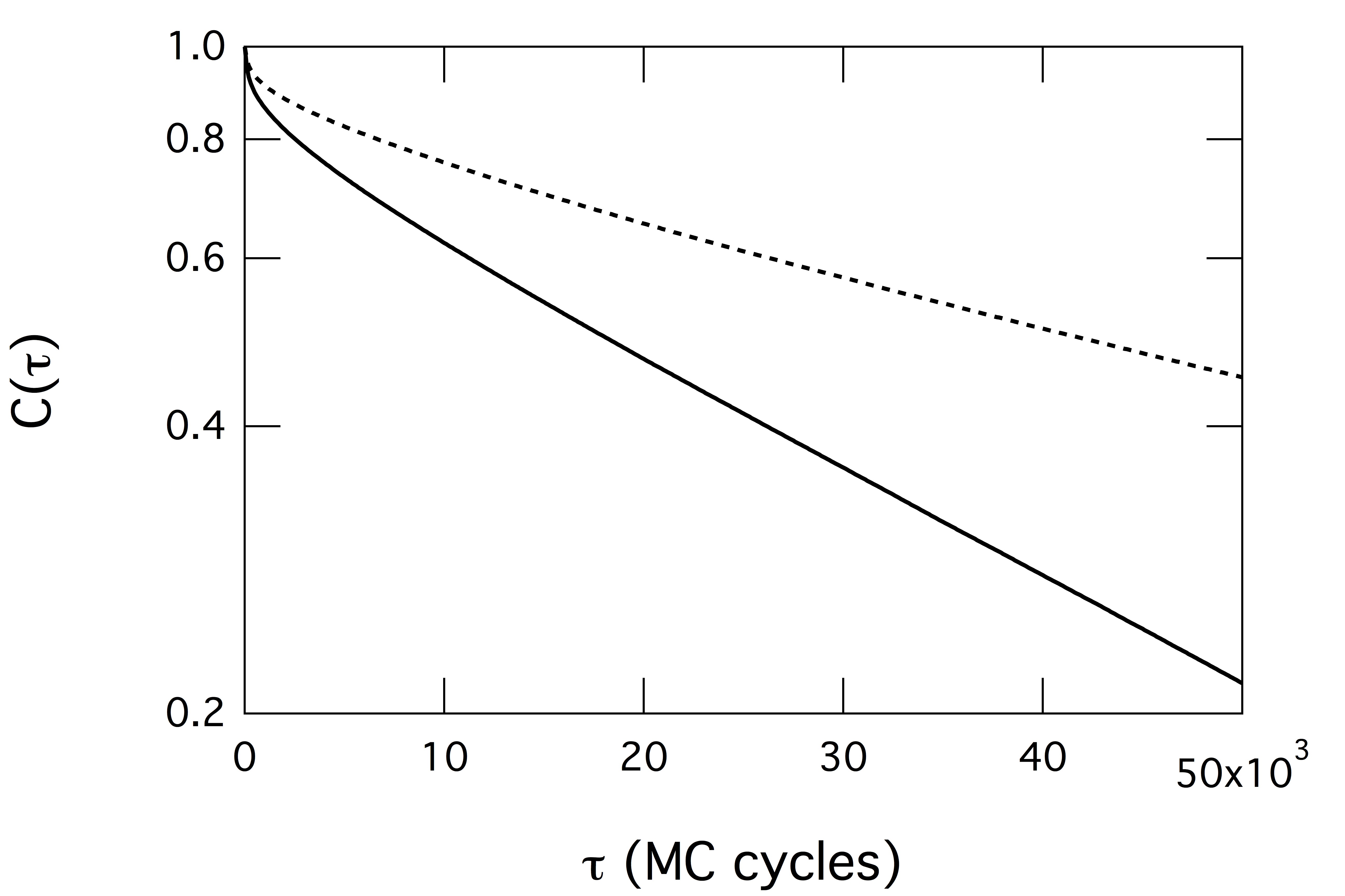
Figure 1: Orientational autocorrelation function $C(\tau)$ for an isotropic fluid of sticky cylinders with aspect ratio $L/D=0.5$ and binding energy $\beta E_{\rm bond}=12$ at a pressure of $\beta PD^{3}=0.8$. Results are shown for simulations with (solid curve) and without (dashed curve) cluster MC moves. Cluster moves decrease the orientational decorrelation time by approximately a factor of two.

II.1.2 Overlap test.  

The test for cylinder-cylinder overlaps is more time-consuming than the corresponding test for hard spheres, spherocylinders or ellipsoids. We use a procedure similar to that used in previous simulation studies of hard cylinders Blaak et al. (1999); Ibarra-Avalos et al. (2007), and that consists of three tests: 1. Spherocylinder overlap: test for overlaps between the enclosing spherocylinders (obtained by adding hemispherical endcaps to hard cylinders). If the spherocylinders don’t overlap, then neither do the hard cylinders. 2. Disk-disk overlap: if an overlap is found in the first step, test for overlaps between the flat end faces of the cylinders. 3. Disk-cylinder overlap: if no overlaps are found in the second step, test for overlaps between the flat end faces of one cylinder and the cylindrical surface of the other.

If the enclosing spherocylinders overlap, but no cylinder-cylinder overlaps are found, then the two cylinders may interact via the short-range attractive potential (Eq. (1)). Computing the attractive interaction between sticky cylinders requires minimal additional effort, because the distance between the centers of the circular end faces of the cylinders is available from the spherocylinder overlap test.

III Theory

To compare the I-N transition in simulation and theory, we extended the work of van der Schoot and Cates van der Schoot and Cates (1994). This analytic theory considers cylindrical monomers (of length $L$ and diameter $D$) that reversibly assemble into linear aggregates. The form of the free energy is determined from three key assumptions. First, the aggregates are treated as nearly rigid cylinders. The ratio of aggregate length $\ell$ to the persistence length $l_{p}$ is assumed small, $\ell/l_{p}\ll 1$. Second, the aggregates interact via steric repulsion. Only pairwise interactions are taken into account within the second virial approximation, but the Parsons-Lee approximation is used to extend the theory to higher density. Third, the assembly of monomers into aggregates is driven by an energetic penalty $E_{\rm bond}$ for monomers to have free ends. We assume that $E_{\rm bond}$ is independent of the aggregate length $\ell$.

The assumption of nearly rigid aggregates does not hold in our simulations: the results shown in this paper have a ratio of aggregate lengths to persistence length $\ell/l_{p}\sim 1$. We discuss below the limitations of the theory in this flexibility regime.

The work of van der Schoot and Cates considered two-particle interactions in the second virial approximation. Since this approximation is accurate only in the dilute limit, we used the Parsons-Lee approximation to extend the theory to the regime of higher packing fractions Parsons (1979). The Parsons-Lee method effectively inlcudes contributions from higher virial coefficients in the interaction free energy.

The total free energy of the system depends on the density of monomers $\rho_{\ell}({\bf u})$ that belong to a subset of aggregates of contour lengths between $\ell$ and $\ell+d\ell$ and have orientations within the solid angle $\Omega_{\bf u}$ and $\Omega_{\bf u}+d\Omega_{\bf u}$ with respect to some specified direction $\hat{\bf n}$. The monomers have length $L$, diameter $D$, aspect ratio $r=L/D$, and volume $v_{0}=\pi D^{2}L/4$. The free energy per unit volume (in units of $k_{B}T$) is

$$\frac{F}{V} = \int d\ell\,\frac{d\Omega_{\bf u}}{4\pi}\,\frac{L}{\ell}\,\rho_{\ell}({\bf u})\,\left[\log\left(\frac{v_{0}L^{2}}{\ell}\rho_{\ell}({\bf u})\right)-1\right]$$ (3)

$${}-\frac{2L}{3l_{p}}\,\int d\ell\,\frac{d\Omega_{\bf u}}{4\pi}\,[\rho_{\ell}({\bf u})]^{1/2}\nabla^{2}[\rho_{\ell}({\bf u})]^{1/2}$$

$${}+L^{2}\,D\,\eta(\phi)\,\int d\ell_{1}\,d\ell_{2}\,\frac{d\Omega_{{\bf u}_{1}}}{4\pi}\,\frac{d\Omega_{{\bf u}_{2}}}{4\pi}\rho_{\ell_{1}}({\bf u}_{1})\times$$

$$\rho_{\ell_{2}}({\bf u}_{2})|\sin\gamma|+E_{\rm bond}\int d\ell\,\frac{d\Omega_{\bf u}}{4\pi}\,\frac{L}{\ell}\,\rho_{\ell}({\bf u}).$$

All length integrals (over $\ell$) are from zero to infinity and all angular integrals (over $\Omega$) are over $4\pi$ of solid angle. The first term is the free energy of a mixture of ideal gases of aggregates. Aggregates of different lengths and orientations are treated as different chemical species. The second term describes semiflexibility of aggregates; it is a perturbative correction to the orientational degrees of freedom (implicitly included in the first term) due to the flexibility of aggregates Khokhlov and Semenov (1982). The third term describes the excluded-volume interaction between pairs of monomers with relative orientations described by $\cos\gamma\equiv{\bf u}_{1}\cdot{\bf u}_{2}$. The prefactor $\eta(\phi)$ reflects the Parsons-Lee correction for higher virial coefficients Parsons (1979); Cinacchi et al. (2004); Cuetos et al. (2007) based on the Carnahan-Starling expression for the correlation function of hard spheres Carnahan and Starling (1969),

$$\eta(\phi)=\frac{1}{4}\,\left(\frac{4-3\phi}{(1-\phi)^{2}}\right),$$ (4)

where $\phi=\rho v_{0}$ is the packing fraction of monomers. In the usual second-virial approximation $\eta(\phi)=1$. The last term in Eq. (3) is the free energy of polymerization, which is proportional to the total number of aggregates in the system. In writing Eq. (3) we assumed that in equilibrium the distribution of monomers is spatially homogenous and that the conformational degrees of freedom of aggregates decouple from the interaction degrees of freedom.

For a closed system the total number of monomers $N$ is fixed, leading to the normalization condition

$$\int d\ell\,\frac{d\Omega_{\bf u}}{4\pi}\,\rho_{\ell}({\bf u})=\frac{N}{V}.$$ (5)

To determine the I-N phase diagram we take the standard approach of requiring mechanical and diffusive equilibrium of the two phases at coexistence. We calculate the osmotic pressure $p^{(i,n)}$ and chemical potential per monomer $\mu^{(i,n)}$ in each phase. Coexistence requires

$$p^{(i)}=p^{(n)},\quad\mu^{(i)}=\mu^{(n)}.$$ (6)

The solution of Eqs. (6) provides information about the packing fractions $\phi^{(i)}$ and $\phi^{(n)}$ of monomers at the coexistence boundaries, the mean aggregation number $\langle n\rangle$ (and distribution of aggregation numbers), as well as the order parameter $S=\frac{1}{2}(\langle 3\cos^{2}\theta\rangle-1)$, where $\theta$ is the angle between the monomer’s axis and the director $\hat{\bf n}$, and averaging is performed over all monomers in the system.

In the sections below we outline the calculations and resulting equations for the isotropic and nematic phases as well as the numerical methods.

III.1 Isotropic phase

In the isotropic phase the monomers are distributed uniformly both in space and in orientation, so $\rho^{(i)}_{\ell}({\bf u})=\rho_{\ell}^{(i)}$ independent of angle. The free energy functional Eq. (3) for the total free energy of the system in the isotropic phase reduces to

$$f^{(i)} \equiv F^{(i)}\cdot\frac{v_{0}}{V}=\int d\ell\,\frac{L}{\ell}\rho^{(i)}_{\ell}\left[\log\Big{(}\frac{v_{0}L^{2}}{\ell}\rho^{(i)}_{\ell}\Big{)}-1\right]$$ (7)

$${}+r\eta(\phi)\phi^{2}+E_{\rm bond}\int d\ell\frac{L}{\ell}\rho^{(i)}_{\ell},$$

where the monomer aspect ratio $r=L/D$ and the monomer packing fraction $\phi=\rho v_{0}$.

Functional minimization of the free energy is subject to the normalization condition Eq. (5), which can be handled with a Lagrange multiplier $\lambda$:

$$\frac{\delta(f^{(i)}+\lambda\int d\ell\rho_{\ell}^{(i)})}{\delta\rho^{(i)}_{\ell}}=0.$$ (8)

This results in a length distribution of aggregates that is, as assumed, independent of orientation

$$\rho^{(i)}_{\ell}=\frac{\ell\,\phi}{v_{0}L^{2}M_{0}^{2}}\,e^{-\ell/(LM_{0})},$$ (9)

with

$$M_{0}=\sqrt{\phi}e^{E_{\rm bond}/2}.$$ (10)

This solution corresponds to an exponential distribution for the density of aggregates $N^{(i)}_{\rm agg}(\ell)/V$ as a function of aggregate length $\ell$:

$$\frac{N^{(i)}_{\rm agg}(\ell)}{V}=\frac{L}{\ell}\rho_{\ell}^{(i)}=\frac{\phi}{v_{0}LM_{0}^{2}}\,e^{-\ell/(LM_{0})}.$$ (11)

The chemical potential per monomer is given by

$$\mu^{(i)}=\frac{\partial f^{(i)}}{\partial\phi}=r\,\phi\,(2\eta(\phi)+\phi\,\eta^{\prime}(\phi))-\frac{e^{-E_{\rm bond}/2}}{\sqrt{\phi}},$$ (12)

where $\eta^{\prime}(\phi)$ is the derivative of $\eta(\phi)$ with respect to $\phi$. The osmotic pressure is

$$p^{(i)} = -\frac{1}{v_{0}}(f^{(i)}-\phi\mu^{(i)})=\frac{1}{v_{0}}\Big{[}r\,\phi^{2}\,(\eta(\phi)+\phi\,\eta^{\prime}(\phi))$$ (13)

$${}+e^{-E_{\rm bond}/2}\,\sqrt{\phi}\,\Big{]}.$$

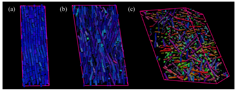
Figure 2: Instantaneous configurations from $NPT$ MC simulations of $N=1440$ $L/D=2$ sticky cylinders with binding energy $\beta E_{\rm bond}=12$ in various phases: (a) columnar LC phase, $\beta PD^{3}=0.7$; (b) nematic phase, $\beta PD^{3}=0.28$; (c) isotropic fluid phase, $\beta PD^{3}=0.18$. Cylinder color encodes orientation: the RGB color index of cylinder $i$ is $(|\hat{u}_{ix}|,|\hat{u}_{iy}|,|\hat{u}_{iz}|$), where $\hat{\bf u}_{i}$ is a unit vector along the cylinder axis.

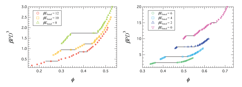
Figure 3: Equation of state for $L/D=1$ measured on expansion from a high-density columnar crystal state (symbols). The horizontal lines indicate the approximate location of first-order phase transitions.

III.2 Nematic phase

In the nematic phase the system is spatially homogenous but orientationally ordered due to alignment of aggregates along a spontaneously chosen direction $\hat{\bf n}$. The system preserves azimuthal symmetry with respect to rotations about $\hat{\bf n}$. Therefore, in spherical coordinates the density $\rho_{\ell}({\bf u})$ is independent of the polar angle $\varphi$ and

$$\int\frac{d\Omega_{\bf u}}{4\pi}\,\rho_{\ell}({\bf u})=\frac{1}{2}\int_{-1}^{1}dx\,\rho_{\ell}(x),$$ (14)

with $x=\cos\theta$, where $\theta$ is the angle to the director $\hat{\bf n}$. As in the previous section, we minimize the system’s free energy with respect to the orientation-dependent density function $\rho_{\ell}(x)$,

$$\frac{\delta(F^{(n)}+\lambda\int d\ell\int_{-1}^{1}dx\rho_{\ell}(x))}{\delta\rho_{\ell}(x)}=0.$$ (15)

This results in the integro-differential equation

$$0 = \lambda+\frac{E_{\rm bond}}{2}\,\frac{L}{\ell}+\frac{1}{2}\,\frac{L}{\ell}\log\left(\frac{v_{0}L^{2}}{\ell}\rho_{\ell}(x)\right)$$ (16)

$$- \frac{L}{3l_{p}}\,\frac{\partial^{2}_{x}[\rho_{\ell}(x)]^{1/2}}{[\rho_{\ell}(x)]^{1/2}}+\frac{L^{2}D\,\eta(\phi)}{2}\times$$

$$\int d\ell^{\prime}\int_{-1}^{1}dx^{\prime}\rho_{\ell^{\prime}}(x^{\prime})\,K(x^{\prime},x).$$

The interaction kernel is

$$K(x_{1},x_{2})=\int_{0}^{2\pi}\frac{d\phi_{1}}{2\pi}\frac{d\phi_{2}}{2\pi}|\sin\gamma|.$$ (17)

Solving Eq.(16) for the function $\rho_{\ell}(x)$ that minimizes the free energy is a difficult task that requires either numerical solution or introduction of a trial function. We chose a mixed approach that starts with a trial function and uses numerical solution of the resulting algebraic equations. We adopted the trial function proposed in reference van der Schoot and Cates (1994):

$$\rho^{(n)}_{\ell}(x)=\frac{\ell\phi}{v_{0}L^{2}M_{0}^{2}}e^{-\ell/(LM(x))},$$ (18)

where the parameter $M_{0}$ is given by Eq. (10) and $M(x)$ is an orientation-dependent aggregation number.

The free energy of the nematic phase as a functional of $M(x)$ becomes

$$f^{(n)} \equiv F^{(n)}\cdot\frac{v_{0}}{V}=-\frac{\phi}{M_{0}}\int_{-1}^{1}dx\,\bar{M}(x)$$ (19)

$${}{}+\frac{r\phi^{2}}{\pi}\int_{-1}^{1}\!\!\int_{-1}^{1}dx_{1}dx_{2}\bar{M}^{2}(x_{1})\,\bar{M}^{2}(x_{2})\,K(x_{1},x_{2})$$

$$-\frac{\phi}{6\bar{l}_{p}}\int_{-1}^{1}dx\bar{M}(x)\partial_{x}^{2}\,\bar{M}(x).$$

The bars denote dimensionless variables: $\bar{l}_{p}=l_{p}/L$ and $\bar{M}(x)\equiv M(x)/M_{0}$. The next step is functional minimization of the free energy to determine an integro-differential equation for $\bar{M}(x)$. We find a series solution for $\bar{M}(x)$ by expanding in Legendre polynomials, which turns the equation for $\bar{M}(x)$ into a system of algebraic equations that we solve numerically. For details of the calculations, see Appendix A. Here we summarize our results for the chemical potential per monomer $\mu^{(n)}$ and osmotic pressure $p^{(n)}$ in the nematic phase:

$$\mu^{(n)} = \frac{\partial f^{(n)}}{\partial\phi}=-\frac{e^{-E_{\rm bond}/2}}{2\sqrt{\phi}}\,I_{1}-\frac{1}{6\bar{l}_{p}}\,I_{2}$$ (20)

$${}+\frac{\phi r}{\pi}(2\eta(\phi)+\phi\eta^{\prime}(\phi))I_{3}$$

$$p^{(n)} = -\frac{1}{v_{0}}(f^{(n)}-\phi\mu^{(n)})=\frac{1}{v_{0}}\Big{[}\frac{\sqrt{\phi}}{2}\,e^{-E_{\rm bond}/2}I_{1}$$ (21)

$${}+\frac{\phi^{2}\,r}{\pi}(\eta(\phi)+\phi\eta^{\prime}(\phi))I_{3}\,\Big{]},$$

where $I_{1}$–$I_{3}$ are integrals involving $\bar{M}(x)$ that are defined in Eqs. (33)-(35).

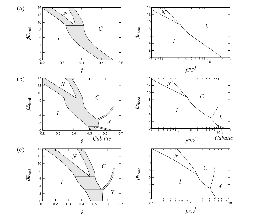
Figure 4: Phase diagrams of the sticky cylinder system as a function of binding energy and packing fraction (left) and binding energy and pressure (right), for aspect ratios $L/D=0.5$ (a), $L/D=1$ (b), and $L/D=2$ (c). A variety of phases are observed, including isotropic ($I$), nematic ($N$), columnar liquid crystal ($C$), columnar crystal ($X$), and cubatic-like ($Cubatic$) phases. Shaded areas correspond to regions of two-phase coexistence.

The mean aggregation number in the nematic phase is

$$\langle n\rangle=\frac{1}{L}\frac{\int d\ell\,\ell\,N^{(n)}_{\rm agg}(\ell)}{\int d\ell N^{(n)}_{\rm agg}(\ell)},$$ (22)

where

$$N^{(n)}_{\rm agg}(\ell)=(L/\ell)\int_{-1}^{1}\rho^{(n)}_{\ell}(x)dx.$$ (23)

is the distribution function of aggregates of length $\ell$ in the nematic phase. The order parameter of aggregates of length $\ell$ is

$$S_{\ell}=\frac{\int_{-1}^{1}dxP_{2}(x)\rho_{\ell}(x)}{\int_{-1}^{1}dx\rho_{\ell}(x)},$$ (24)

where $P_{2}(x)$ is the second-order Legendre polynomial. The order parameter (averaged over all monomers in the system) is

$$S=\frac{\int d\ell\int_{-1}^{1}dxP_{2}(x)\rho_{\ell}(x)}{\int d\ell\int_{-1}^{1}dx\rho_{\ell}(x)}.$$ (25)

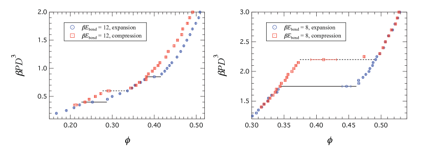
Figure 5: Hysteresis in the equation of state for $L/D=1$ with $\beta E_{\rm bond}=12$ (left) and $\beta E_{\rm bond}=8$ (right). The horizontal lines indicate the approximate location of first-order phase transitions observed on expansion from a high-density columnar crystal state (solid lines) and on compression from a low-density isotropic fluid state (dashed lines).

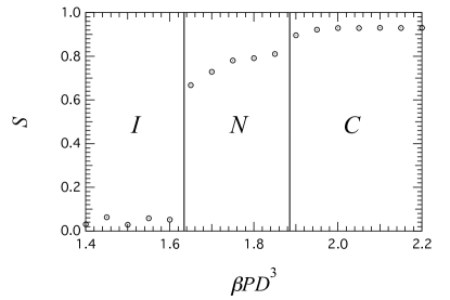
Figure 6: Nematic order parameter $S$ as a function of pressure for $L/D=0.5$ and $\beta E_{\rm bond}=10$.

IV Simulation results

In Figure 2 we illustrate the phase behavior with sample snapshots of the simulations. Instantaneous configurations from simulations of the $L/D=2$ sticky-cylinder system with binding energy $\beta E_{\rm bond}=12$ are shown. This figure displays the typical phase sequence observed upon expansion from a high-density columnar crystal for large binding energy, which includes the columnar LC phase, the nematic phase, and the isotropic fluid phase.

To determine phase boundaries, we determined the locations of plateaus in the equation of state obtained on expansion from a high density columnar crystal state. Such plateaus indicate first-order phase transitions. Phase identification was based on structural properties such as the pair-correlation function and nematic order parameter, as discussed below. For example, the equation of state for $L/D=1$ and various values of $\beta E_{\rm bond}$ is shown in Figure 3, with the approximate location of first-order phase transitions indicated by horizontal solid lines.

Phase diagrams of the sticky-cylinder system for aspect ratios $L/D=0.5$, 1 and 2 are shown in Figure 4. All three phase diagrams share the same key features. First, both nematic ($N$) and columnar LC ($C$) phases are observed for large $\beta E_{\rm bond}$. The range of nematic stability (in terms of pressure or packing fraction) increases with increasing binding energy. Second, an isotropic-nematic-columnar triple point is observed at intermediate binding energies. For binding energies below the triple point, there is a direct transition from the isotropic phase to the columnar LC phase.

We also find a columnar crystal ($X$) phase at high density, and the $L/D=1$ system exhibits a cubatic-like phase for small $\beta E_{\rm bond}$. The cubatic-like phase was previously described by Blaak et al. Blaak et al. (1999) in the $L/D=0.9$ hard cylinder system. As the focus of this paper is on LC phases, we have not investigated the crystalline or cubatic phases in detail, and the phase boundaries involving these phases should be regarded as schematic.

Comparison of the equation of state obtained on compression from an isotropic fluid state with that obtained on expansion from a high-density columnar crystal state reveals considerable hysteresis (Figure 5). This hysteresis becomes increasingly pronounced with decreasing $\beta E_{\rm bond}$, and compression from the low-density isotropic state for small $\beta E_{\rm bond}$ typically leads to a high-density disordered (jammed) state, likely due to the dominance of hard-core interactions in this limit. For large $\beta E_{\rm bond}$, the I-N transition occurs at relatively low packing fractions, which facilitates annealing into a well-ordered nematic state starting from an isotropic state. Because we generally observed slow kinetics of formation of an ordered state starting from disordered (isotropic) initial configuration, we used isotherms obtained on expansion (e.g., Figure 3) to construct the phase diagrams in Figure 4. This implies that the phase boundaries shown are lower limits (both in density and pressure), and should be considered provisional. In future work we will refine the phase diagram using free energy calculations.

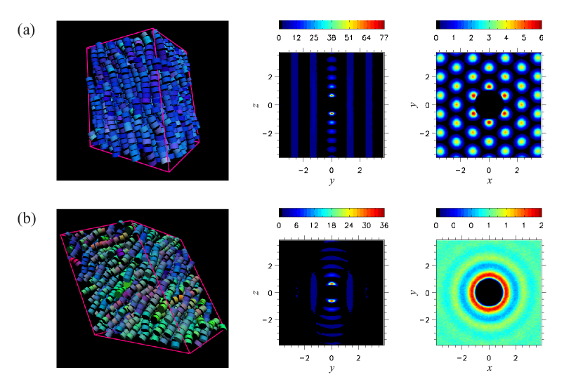
Figure 7: Instantaneous configurations (left) and pair distribution functions in planes containing the nematic director $\hat{\bf z}\equiv\hat{\bf n}$ ($g(0,y,z)$, center) and perpendicular to the nematic director ($g(x,y,0)$, right) for $L/D=0.5$ and $\beta E_{\rm bond}=12$. (a) Columnar LC phase at $\beta PD^{3}=1.8$, obtained by expansion from a high-density columnar crystal. There are no long-range correlations in the $z$ positions of cylinders, as shown by $g(0,y,z)$, and a well-defined hexagonal lattice of columns is apparent in $g(x,y,0)$. (b) Nematic LC phase at $\beta PD^{3}=1.1$, obtained by compression from a low-density isotropic fluid. Again, there are no long-range correlations in the $z$ positions of cylinders, as shown by $g(0,y,z)$. The plot of $g(x,y,0)$ reveals isotropic and rapidly decaying positional correlations in the plane perpendicular to $\hat{\bf z}$, indicative of nematic order.

IV.1 Order parameter and correlation functions

We measured nematic order by calculating the tensor

$$Q_{\alpha\beta}={1\over N}\sum_{i=1}^{N}\left({3\over 2}\hat{u}_{i\alpha}\hat{u}_{i\beta}-{1\over 2}\delta_{\alpha\beta}\right),$$ (26)

where $\alpha$ and $\beta$ refer to cartesian components, $i$ indexes the sum over monomers, and $\delta_{\alpha\beta}$ is the Kronecker delta function. The nematic order parameter $S$ is the largest eigenvalue of the average order tensor $\langle Q_{\alpha\beta}\rangle$, and the nematic director $\hat{\bf n}$ is the corresponding eigenvector. Typical results for $S$ as a function of pressure are shown in Figure 6, for $L/D=0.5$ and $\beta E_{\rm bond}=10$. The order parameter jumps abruptly from a small value ($S\approx 0.05$) in the isotropic phase to $S\approx 0.7-0.8$ in the nematic phase, and exhibits a further abrupt jump to $S\approx 0.9$ in the columnar LC phase. We list values of the nematic order parameter in the nematic or columnar liquid crystal phases at coexistence ($S_{N}$ or $S_{C}$) with the isotropic phase in Table 1. The values of $S$ are generally large ($>0.7$), indicating a high degree of orientational order in all LC phases investigated.

To distinguish between the various orientationally ordered phases we computed the three-dimensional pair distribution function $g({\bf r})$ and examined positional correlations as a function of pair separations parallel and perpendicular to the nematic director. The pair distribution function $g({\bf r})$ is defined as the normalized probability of finding a pair of particles with separation ${\bf r}$,

$$g({\bf r})={1\over{\rho N}}\left\langle\sum_{i=1}^{N}\sum_{j\neq i}\delta({\bf r}+{\bf r}_{j}-{\bf r}_{i})\right\rangle,$$ (27)

where $\rho=N/V$ is the average number density of particles and $\delta({\bf r})$ is the Dirac delta function.

Figure 7 shows example plots of pair distribution functions. The nematic director defines the $z$ direction ($\hat{\bf z}\equiv\hat{\bf n}$), so $g(0,y,z)$ is in a plane containing the nematic director and $g(x,y,0)$ is in a plane perpendicular to the nematic director. For this set of simulations, $L/D=0.5$ and $\beta E_{\rm bond}=12$. The columnar LC phase shown in Figure 7(a) is characterized by a well-defined hexagonal lattice of columns and by the absence of long-range correlations in the $z$ positions of cylinders. The nematic LC phase shown in Figure 7(b) exhibits isotropic and rapidly decaying positional correlations in the plane perpendicular to $\hat{\bf n}$.

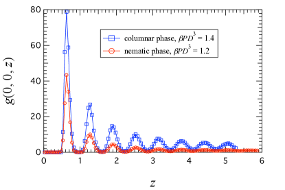
Figure 8: One-dimensional pair distribution function $g(0,0,z)$ along a line parallel to the nematic director in the columnar LC phase (blue squares) and the nematic phase (red circles) for $L/D=0.5$ and $\beta E_{\rm bond}=12$.

We computed the positional correlation length $\xi_{\parallel}$ along the nematic director in both the nematic and columnar LC phases from the one-dimensional pair distribution function along a line parallel to the nematic director, $g(0,0,z)$. Figure 8 shows typical results for the columnar LC and nematic phases for $L/D=0.5$ and $\beta E_{\rm bond}=12$. We find exponential decay of correlations to a constant in both phases (in the nematic phase $g(0,0,z)$ approaches 1 for large $z$, while in the columnar LC phase we estimated that $g(0,0,z)$ approaches 3.5 for large $z$). The correlation length determined by fitting the exponential decay is $\xi_{\parallel}=1.3$ in the nematic phase at $\beta PD^{3}=1.2$ and $\xi_{\parallel}=1.8$ in the columnar LC phase at $\beta PD^{3}=1.4$. In the same simulations, the mean aggregate lengths are 44 in the nematic phase and 352 in the columnar LC phase. This gives a ratio of aggregate length to correlation length that is large: $\ell/\xi_{\parallel}\approx 33$ in the nematic phase and $\ell/\xi_{\parallel}\approx 200$ in the columnar LC phase. (For more discussion of aggregate lengths, see Section IV.2 below.) In other words, we find that the correlation length can differ from the mean aggregate length by 1-2 orders of magnitude. This in turn suggests that it may not be feasible to determine the mean aggregation number from X-ray scattering experiments that measure correlation lengths, such as the experiments of references Park et al. (2008); Joshi et al. (2009).

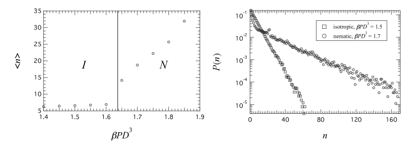
Figure 9: Mean aggregation number $\langle n\rangle$ as a function of pressure (left) and aggregation number distributions $P(n)$ (right) for $L/D=0.5$ and $\beta E_{\rm bond}=10$, measured on expansion from a high-density columnar crystal state. The nematic phase $P(n)$ displays fast exponential decay for small $n$ crossing over to slow exponential decay for large $n$ (bi-exponential distribution). The small peak near $n=20$ in the nematic aggregation number distribution is a finite-size artifact, associated with aggregates that connect to themselves across the periodic boundaries.

IV.2 Aggregate Statistics

We measured the aggregation number distribution function $P(n)$ and its first moment, the mean aggregation number $\langle n\rangle$, in the isotropic, nematic, and columnar LC phases. Here $n$ is the aggregation number (the number of monomers in an aggregate). Aggregates are defined by proximity: any pair of cylinders with endpoint separation smaller than $r_{c}$ belongs to the same aggregate.

The use of a finite simulation volume imposes a cutoff on the aggregate-length distribution. This finite-size effect is particularly evident in the limit of large binding energies, where the mean aggregate length can exceed the maximum linear dimension of the periodic simulation cell. To ameliorate this effect, the initial columnar crystal configurations used for expansion runs were constructed with an oblique orientation of columns with respect to the edge vectors of the periodic simulation cell, so that a given column traverses the periodic box multiple times before intersecting itself. With this expedient, we are able to measure aggregation number distributions over a wide range of conditions, although small finite-size artifacts associated with aggregates that connect to themselves across the periodic boundaries are observed in many of the expansion runs (see Figure 9).

We illustrate the typical aggregation behavior in Figure 9, which shows the mean aggregation number $\langle n\rangle$ as a function of pressure (left) and aggregation number distributions $P(n)$ in the isotropic and nematic states (right) for $L/D=0.5$ and $\beta E_{\rm bond}=10$, measured upon expansion from a high-density columnar crystal state. The mean aggregation number jumps discontinuously at the I-N transition, and increases strongly with increasing pressure in the nematic phase. This behavior is qualitatively consistent with that observed in previous simulation and theoretical studies of semiflexible linear aggregates. The distribution $P(n)$ has an exponential dependence on $n$ in the isotropic phase, but displays biexponential behavior in the nematic phase, i.e., fast exponential decay for small $n$ crossing over to slow exponential decay for large $n$. Such biexponential behavior has been noted previously by Lü and Kindt Lu and Kindt (2004), who argued that the short length scale behavior of $P(n)$ comes from a distinct population of short aggregates with relatively low orientational order. Biexponential behavior in the nematic phase is also predicted by the analytic theory; see Figure 11. In the simulations we also observed a biexponential aggregation number distribution in the columnar LC phase.

Mean aggregation numbers in the isotropic phase at coexistence ($\langle n\rangle_{I}$) and in the nematic or columnar LC phase at coexistence with the isotropic phase ($\langle n\rangle_{N}$ or $\langle n\rangle_{C}$) are listed in Table 1. The mean aggregation number at coexistence tends to increase with increasing $\beta E_{\rm bond}$, although the trend in the nematic or columnar LC phase at coexistence isn’t strictly monotonic. We note that the mean aggregation numbers at coexistence decrease with increasing cylinder aspect ratio for a given $\beta E_{\rm bond}$, possibly because the corresponding packing fractions at coexistence decrease with increasing aspect ratio.

Table 1: Properties of the sticky-cylinder system measured in $NPT$ MC simulations. Columns contain the cylinder aspect ratio $L/D$, the dimensionless binding energy $\beta E_{\rm bond}$, the number of particles $N$, the measured persistence length $l_{p}$, the mean intra-aggregate bond length $\langle R\rangle$, the mean aggregation number in the isotropic phase at coexistence $\langle n\rangle_{I}$, the mean aggregation number in the nematic or columnar LC phase at coexistence with the isotropic phase ($\langle n\rangle_{N}$ or $\langle n\rangle_{C}$), and the nematic order parameter in the nematic or columnar phase at coexistence with the isotropic phase ($S_{N}$ or $S_{C}$).

$L/D$	$\beta E_{\rm bond}$	$N$	$l_{p}$	$\langle R\rangle$	$\langle n\rangle_{I}$	$\langle n\rangle_{N}$	$\langle n\rangle_{C}$	$S_{N}$	$S_{C}$
0.5	12	1920	14.9	0.66	9.96	24.08	-	0.704	-
	10	1680	13.5	0.67	6.91	18.75	-	0.729	-
	8	1680	11.4	0.68	4.06	-	45.90	-	0.908
	6	1440	9.2	0.69	2.74	-	27.44	-	0.895
	4	1440	7.2	0.70	2.10	-	15.85	-	0.872
	2	1200	5.4	0.70	1.78	-	14.96	-	0.869
	0	1200	-	-	-	-	-	-	-
1	12	1440	31.4	1.15	5.65	14.98	-	0.761	-
	10	1200	27.3	1.16	4.15	16.38	-	0.841	-
	8	1200	22.3	1.17	2.83	-	58.42	-	0.947
	6	1200	17.7	1.17	1.89	-	12.95	-	0.903
	4	960	13.3	1.18	1.55	-	11.04	-	0.902
	2	960	-	-	-	-	-	-	-
	0	720	-	-	-	-	-	-	-
2	12	1440	62.6	2.14	3.80	11.88	-	0.840	-
	10	1200	51.0	2.15	2.54	11.15	-	0.873	-
	8	1200	44.4	2.16	1.82	7.99	-	0.870	-
	6	960	32.2	2.16	1.43	-	19.58	-	0.965
	4	960	24.3	2.17	1.22	-	9.31	-	0.956
	2	720	-	-	-	-	-	-	-
	0	720	-	-	-	-	-	-	-

IV.3 Persistence Length

As discussed above, the persistence length of sticky-cylinder aggregates is determined by cylinder-cylinder interactions. We measured the persistence length from the bond orientational correlation function,

$$C_{O}(s)=\left\langle\hat{\bf R}_{i}\cdot\hat{\bf R}_{i+m}\right\rangle,$$ (28)

where $\hat{\bf R}_{i}$ is a unit vector along the $i$th bond (the vector joining the centers of two neighboring cylinders) in an aggregate, the contour length $s=m\langle R\rangle$, and $\langle R\rangle$ is the average bond length. In the isotropic phase, $C_{O}(s)$ decays exponentially with increasing $m$, with a decay constant that can be identified with the persistence length $l_{p}$, $C_{O}(s)=\exp(-s/l_{p})$. By fitting this exponential decay to the simulation data, we determined the persistence length. For a given $L/D$ and $\beta E_{\rm bond}$, we find that the calculated persistence length is nearly independent of pressure within the isotropic phase, which gives us confidence that this procedure measures the intrinsic bending rigidity of aggregates. Table 1 lists the persistence length and average bond length as a function of $L/D$ and $\beta E_{\rm bond}$, where both quantities are averaged over isotropic state points.

The persistence length increases approximately linearly with increasing binding energy, and is also approximately proportional to cylinder aspect ratio $L/D$ for a given binding energy. Because of this, the reduced persistence length $\bar{l}_{p}=l_{p}/L$ is reasonably well approximated as a universal linear function of $\beta E_{\rm bond}$, independent of cylinder aspect ratio, as shown in Figure 10. The solid line in Figure 10 is the best linear fit to the data, $\bar{l}_{p}=5.07+2.14\beta E_{\rm bond}$. The ratio of persistence length to monomer length approaches a nonzero constant in the limit of zero binding energy. This indicates that there is a significant entropic contribution to the persistence length due to hard-core interactions between neighboring cylinders in an aggregate.

Figure 10: Ratio of persistence length to monomer length $\bar{l}_{p}=l_{p}/L$ as a function of $\beta E_{\rm bond}$ for aspect ratios $L/D=0.5$ (circles), $L/D=1$ (squares), and $L/D=2$ (triangles). The data for all three aspect ratios is well approximated by a universal linear function, $\bar{l}_{p}=5.07+2.14\beta E_{\rm bond}$, which represents the best linear fit to the data (solid line).

We expect that the precise way that $\bar{l}_{p}$ varies with $\beta E_{\rm bond}$ to depend strongly on the form of the intermolecular potential. This dependence can be estimated by simple dimensional analysis arguments. When two bound cylinders interact, thermal fluctuations will typically cause their separation to vary to about 1 $k_{B}T$ above their minimum interaction energy $E_{\rm min}=-E_{\rm bond}$. Therefore a typical separation $r_{t}=R/\sqrt{\beta E_{\rm bond}}$. This suggests a characteristic angle defined by the distance $r_{t}$ and the cylinder radius $R$: $\tan\theta=r_{t}/R=1/{\sqrt{\beta E}}$. The typical angle is therefore $\cos\theta=1/\sqrt{1+1/(\beta E_{\rm bond})}$. This gives an estimate of the persistence length, based on the relation $\langle\cos\theta\rangle=e^{-L/l_{p}}$ and assuming $\beta E_{\rm bond}\gg 1$, of $\bar{l}_{p}=2\beta E_{\rm bond}$. In other words, the persistence length should vary linearly with $\beta E_{\rm bond}$, with a slope of 2, as observed in simulations.

For other forms of the potential, this dependence would change. Using the same dimensional analysis argument, we would predict that for an exponent of $\gamma$ in the interaction potential (Eqn. (1)), the scaling is $\bar{l}_{p}=2(\beta E_{\rm bond})^{2/\gamma}$. In the limit of a square well ($\gamma\to\infty$) the persistence length would become independent of $\beta E_{\rm bond}$. Because the phase behavior of aggregates is strongly dependent on the persistence length, this implies a strong dependence of the phase behavior on the form of the monomer-monomer interaction potential, in addition to the obvious dependence on the binding energy. In the future it would be interesting to investigate the interplay of these two effects, focusing how sticky-cylinder phase behavior varies with the form of the interaction potential.

The aggregates in this study are relatively flexible: the ratio of persistence length to mean aggregate length for the nematic phase at coexistence ranges from $\approx 0.8$ for $L/D=0.5$ and $\beta E_{\rm bond}=12$ to $\approx 2.9$ for $L/D=2$ and $\beta E_{\rm bond}=12$.

V Theory-simulation comparison

We compared our analytic theory results both to the simulations of Lü and Kindt Lu and Kindt (2004) and to our simulations. These comparison illustrate the key role of aggregate flexibility in determining the theory-simulation agreement.

Figure 11: Theoretical predictions of aggregate length and order parameter distributions. Top, aggregate length distributions at I-N coexistence of the isotropic (I, dashed curves) and nematic (N, solid curves) phases with $\bar{l}_{p}=1000$ and $\bar{l}_{p}=100$ (subscripts). Note that in this figure the predictions of the simple second-virial approximation and the Parsons-Lee approximation overlap. Bottom, length-dependent aggregate order parameter at I-N coexistence in the nematic phase with $\bar{l}_{p}=1000$ and $\bar{l}_{p}=100$ (subscripts). Solid curves: simple second-virial approximation. Dashed curves: Parsons-Lee approximation. In both cases, the association constant $K=e^{\beta E_{\rm bond}}=5000$, for comparison with the simulations of Lü and Kindt Lu and Kindt (2004).

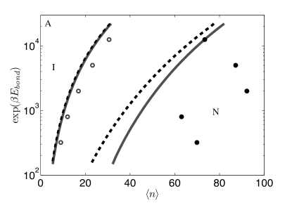
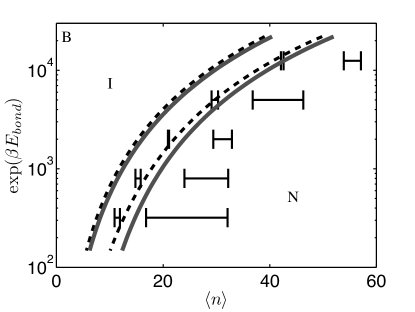
Figure 12: Theoretical predictions of mean aggregation number in the isotropic and nematic phases at I-N coexistence. (A), $\bar{l}_{p}=1000$. (B), $\bar{l}_{p}=100$. Comparison of theory (solid and dashed curves) to simulation results of Lü and Kindt Lu and Kindt (2004) (points). Curves denote borders of regions of I-N coexistence. Solid curves: simple second-virial approximation. Dashed curves: Parsons-Lee approximation. Points and bars: simulation results of Lü and Kindt Lu and Kindt (2004). Note that for $\bar{l}_{p}=100$ (B) Lü and Kindt gave ranges of measured values, which we plot using horizontal bars, while for $\bar{l}_{p}=1000$ (A) Lü and Kindt gave only mean values, which we plot using points.

First, we calculated the aggregate length distributions and order parameter as a function of length to compare with the simulation results of Lü and Kindt (Figure 11). Lü and Kindt considered two persistence length values, $\bar{l}_{p}=1000$ and $\bar{l}_{p}=100$ Lu and Kindt (2004). Note that $\bar{l}_{p}=l_{p}/L$ is the persistence length divided by the monomer length. (In Lü and Kindt’s work, the monomers are spheres.) For this figure, we used the the association constant $K=e^{\beta E_{\rm bond}}=5000$.

A significant and unexpected result is the calculated biexponential aggregate length distribution in the nematic phase. This distribution arises naturally from the free-energy minimization (Figure 11, top). To our knowledge, our work is the first to find this biexponential distribution in analytic theory. Lü and Kindt’s initial analytic work found only a single exponential distribution Lu and Kindt (2004); in later work they found that assuming a biexponential distribution improved the theory-simulation agreement Lu and Kindt (2006).

Overall we find good quantitative agreement between the predictions of the analytic theory for aggregate length distributions and order parameter as a function of aggregate length (compare Figure 11 to Figure 2 of reference Lu and Kindt (2004)). The aggregate length distribution is exponential in the isotropic phase and biexponential in the nematic phase. The nematic phase also shows significantly longer aggregates. Stiffer aggregates also tend to be longer in the nematic phase. The average alignment depends strongly on aggregate length in the nematic phase, with short aggregates only weakly aligned and a rapid increase in the length-dependent order parameter with aggregate length.

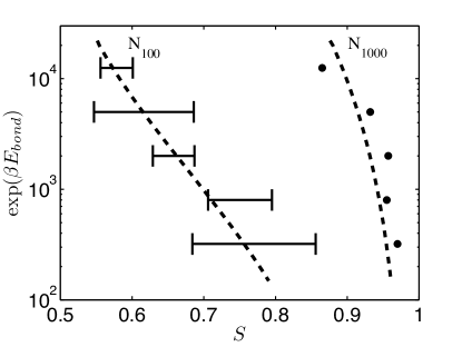
Figure 13: Comparison of nematic order parameter at I-N coexistence predicted by theory (dashed curves) to simulation results of Lü and Kindt Lu and Kindt (2004) (points). Persistence lengths $\bar{l}_{p}=1000$ and $\bar{l}_{p}=100$ indicated by subscripts.

Next we compared our predictions for the aggregate length and nematic order parameter at I-N coexistence to the simulations of Lü and Kindt for a range of monomer binding energies $E_{\rm bond}$. In Figure 12 we plot the average aggregation number in the isotropic and nematic phases at I-N coexistence for a range of values of $E_{\rm bond}$. The curves are predictions of our analytic theory and the bars and points are values from the simulations of Lü and Kindt Lu and Kindt (2004). Note that for the shorter persistence length $\bar{l}_{p}=100$ Lü and Kindt gave ranges of measured values, which we plot using horizontal bars, while for the larger persistence length $\bar{l}_{p}=1000$ Lü and Kindt gave only mean values, which we plot using points. (The same holds for the two figures below in which we compare to Lü and Kindt’s work). This result illustrates the strong enhancement of aggregation in the nematic phase. The theory clearly captures the correct qualitative trends of the simulations: as the binding energy increases, the aggregates become longer in both the isotropic and the nematic phases. Quantitatively agreement is reasonable for the larger persistence length, but for the shorter persistence length $\bar{l}_{p}=100$ the predicted values of $\langle n\rangle$ are off by approximately 50%. This illustrates the decreased quantitative accuracy of the theory as the aggregates become less flexible.

The order parameter in the nematic phase at I-N coexistence is shown in Figure 13. Here our calculations for the order parameter agree well with the simulation results. As expected, the stiffer, longer aggregates show a higher average order parameter that is less sensitive to the binding energy.

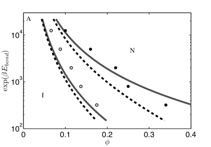
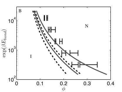
Figure 14: Comparison of theory (solid and dashed curves) to simulation results of Lü and Kindt Lu and Kindt (2004) (points). (A), $l_{p}=1000$. (B), $l_{p}=100$. Curves denote borders of regions of I-N coexistence. Solid curves: simple second-virial approximation. Dashed curves: Parsons-Lee approximation.

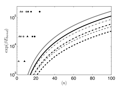
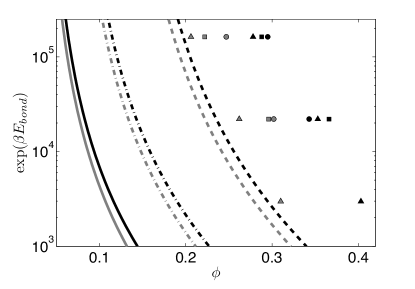
Figure 15: Comparison of I-N coexistence in theory (curves) and simulation (points). Top, aggregation number. Botton, phase diagarm Curves denote borders of regions of I-N coexistence; gray: onset of I-N coexistence; black: upper limit of I-N coexistence. Solid curve: $L/D=2$. Dashed curves: $L/D=1$. Dotted curves: $L/D=0.5$. In doing the calculations we used the empiricial persistence length found from simulations $\bar{l}_{p}=5.07+2.14\beta E_{\rm bond}$. Triangles: $L/D=2$. Squares: $L/D=1$. Circles: $L/D=0.5$.

Our final comparison with the simulation results of Lü and Kindt is the phase diagrams shown in Figure 14. The analytic theory agrees well with the $\bar{l}_{p}=1000$ simulation results and less well with the $\bar{l}_{p}=100$ simulation results. For $\bar{l}_{p}=100$ the analytic theory gives errors of up to about 50% in the predicted volume fraction $\phi$ of the coexistence region. Perhaps surprisingly, we find that the simple second-virial approximation (solid curves in Figure 14) are closer to the simulation results than the results that include the Parsons-Lee approximation (dashed curves).

In our simulations, the ratio of persistence length to monomer length $\bar{l}_{p}=L/D$ is significantly less than in the work of Lü and Kindt; we find values $\bar{l}_{p}\approx 20-30$ in the I-N coexistence range (Table 1). The ratio of mean aggregate length to persistence length $\ell/l_{p}\approx 0.1-1$ in this range (Table 1). Because our analytic theory assumes nearly rigid aggregates ($\ell/l_{p}\ll 1$) we expect that the theory will not show good quantitative agreement with the simulations in this regime. We note that in our simulations the persistence length is not a control parameter but is determined by the balance of binding energy and entropy of the aggregates; we found empirically that $\bar{l}_{p}=5.07+2.14\beta E_{\rm bond}$ (figure 10). We used this empirical relationship in the analytic theory.

In Figure 15 we show the aggregation number and volume fraction at the borders of I-N coexistence. While the qualitative trends in the simulations are correctly captured by theory, there is significant quantitative disagreement. The analytic theory predicts significantly larger aggregation numbers and significantly lower volume fractions than found in the simulations. The biggest discrepancy is with the aggregation numbers, where the analytic theory predictions are larger than found in simulation by factors of 2–5. For the volume fraction, the discrepancy is a factor of 1/3–4. However, we do note that although the position of the phase boundaries is not correctly predicted by our theory, their slope is. We note that the slope is affected by the variation of the persistence length $\bar{l}_{p}$ with $\beta E_{\rm bond}$: including this variation in the analytic theory is necessary to reproduce the slope seen in the simulations.

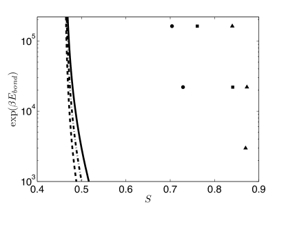
Figure 16: Comparison of order parameter in theory (curves) and simulation (points) in the nematic phase at I-N coexistence. Solid curve: $L/D=2$. Dashed curves: $L/D=1$. Dotted curves: $L/D=0.5$. In doing the calculations we used the empiricial persistence length found from simulations $\bar{l}_{p}=5.07+2.14\beta E_{\rm bond}$. Triangles: $L/D=2$. Squares: $L/D=1$. Circles: $L/D=0.5$.

We also find significant quantitative discrepancy in the order parameter in the nematic phase at coexistence (Figure 16). The theory predicts lower values of $S$ than found in the simulations by almost a factor of 2.

VI Conclusion

Recent experiments on the coupled aggregation and liquid-crystal ordering of chromonic liquid crystals and short double-stranded nucleic acids motivated us to consider coarse-grained simulation and theory of this problem. In nucleic acid systems in particular, the monomer aspect ratio can be varied by varying the number of base pairs per monomer; however, the effects of varying monomer aspect ratio on the aggregation/LC ordering problem have not been extensively studied in theoretical work.

In this paper we used both Monte Carlo simulation and analytic theory to study aggregation and liquid-crystal ordering of a simple model of sticky cylinders. The model assumes hard cylinders (of length $L$ and diameter $D$, so the aspect ratio of the monomers can easily be varied) that experience attractive interactions when they stack end to end.

We determined approximate phase diagrams by using calculations of the equation of state in expansion and compression runs; we then studied the aggregate length distributions, order parameter, and correlation functions in the different phases. We find isotropic, nematic, columnar LC, columnar crystal, and cubatic-like phases are possible for this system. This family of phases is similar to the results of Hentschke and colleagues Fodi and Hentschke (2000); Ouyang and Hentschke (2007) but does show differences with the work of Lü and Kindt, who only observed isotropic and nematic phases Lu and Kindt (2004). Similarly to previous work we observe the disappearance of the nematic phase (as the monomer binding energy drops or temperature increases) at an isotropic-nematic-columnar triple point Taylor and Herzfeld (1991); Fodi and Hentschke (2000); Ouyang and Hentschke (2007); Park et al. (2008); Edwards et al. (2008). These phase diagrams bear a strong qualitative resemblance to those of chromonic liquid crystals, which show a strong decrease in nematic phase width with increasing temperature Park et al. (2008); Edwards et al. (2008). The location of the I-N-C triple point appears to be sensitive to the monomer aspect ratio, occurring at lower $\beta E_{\rm bond}$ for larger $L/D$.

In the simulations we studied three aspect ratios: $L/D=0.5$, 1, and 2. The same qualitative phase behavior is present for all aspect ratios. The key differences are that, first, we only observe the cubatic-like phase for $L/D=1$. This is consistent with previous work on hard cylinders Blaak et al. (1999). Second, we do not observe the columnar crystal phase for the lowest aspect ratio of 0.5. Naïvely this might be understood because having columns made of a larger number of shorter monomers makes the increase in entropy allowed by disorder along the columns more favorable. Third, as noted above, the nematic phase persists to lower $\beta E_{\rm bond}$ when the aspect ratio is larger. Qualitatively, this makes sense. We find that the mean aggregate length at I-N coexistence increases with increasing monomer aspect ratio, which suggests (as in Onsager theory) that the density at coexistence should also decrease with increasing monomer aspect ratio. We do observe this decrease, although the trend is not extremely strong. We also find that the persistence length increases linearly with increasing monomer aspect ratio; therefore aggregate stiffness increases with increasing aspect ratio (assuming fixed binding energy). Both increasing aggregate length and increasing aggregate stiffness tend to favor nematic order, and therefore tend to broaden the nematic region.

Our results give evidence that the phase diagram depends on the the form of the interaction potential, not just the binding energy between monomers. The phase behavior is sensitive to the flexibility of the aggregates, and the aggregate persistence length varies with temperature in a way that is controlled by the interaction potential. This suggests that the temperature dependence of the I-N phase boundary as well as the location of the I-N-C triple point are influenced by the implicit dependence of $l_{p}$ on $\beta E_{\rm bond}$. This is an interesting direction for future work.

Our simulation results demonstrate a remarkable difference between the correlation length along aggregates and the length of aggregates in the nematic and columnar LC phases. Indeed, the aggregate length is typically 10-100 times larger than the density correlation length along the columns. This has important implications for attempts to measure aggregate length distributions: X-ray scattering experiments, which measure correlation lengths, may not be able to probe aggregate lengths Park et al. (2008); Joshi et al. (2009).

In our computations the aggregate persistence length is determined from the interaction potential of the monomers; we found a universal (independent of $L/D$) linear dependence of $\bar{l}_{p}=l_{p}/L$ on $E_{\rm bond}$.

Our extensions of previous theoretical work suggest that quantitative agreement between analytic theory and simulation for the I-N transition of aggregates is within reach. Starting with the relatively simple second-virial model of aggregation and nematic order of van der Schoot and Cates van der Schoot and Cates (1994), we added (1) the Parsons-Lee approximation for higher-density systems, and (2) expansion of the angular trial function in Legendre polynomials and numerical solution of the resulting algebraic equations. This combination significantly improves the quantitative agreement between the analytic theory and the simulations of Lü and Kindt Lu and Kindt (2004).

Our analytic theory predicts the biexponential distribution of aggregate lengths in the nematic phase. Previous analytic work of Lü and Kindt assumed a biexponential distribution in the nematic phase, and based on this assumption found good agreement with their simulation results Lu and Kindt (2006). Here the biexponential distribution arises directly from the free-energy minimization and does not have to be added to the theory as an assumption.

The comparison between simulation and theory highlights the role of aggregate flexibility in controling the phase diagram. In our analytic theory, the aggregates are treated as nearly rigid. Therefore, our theoretical results match the simulation results best where the aggregate persistence length is long ($\bar{l}_{p}=1000$). In this regime, the quantitative agreement between theory and simulation is remarkably good, particularly in the prediction of the phase boundaries, the order parameter, and the biexponential aggregate length distribution in the nematic phase. When comparing to the simulations of Lü and Kindt with shorter aggregate persistence length ($\bar{l}_{p}=100$) or our simulations ($\bar{l}_{p}\approx 20-30$), the quantitative agreement between analytic theory and simulation decreases. Future improvement to the theory will require improved treatment of aggregate flexibility.

A major direction for future research is the comparison of our results to experimental results on chromonic and nucleic-acid liquid crystals, and refinement of both the simulation model and the analytic theory based on the comparison. In the future, improvements to the simulation model and the analytic theory may allow true quantitative agreement between experiment, simulation, and theory.

Appendix A Free energy minimization in the nematic phase

Here we outline the free energy minimization and numerical solution for the function $M(x)$ introduced in Eq. (18). Plugging the trial function Eq. (18) into the normalization condition Eq. (5) we arrive at the normalization condition for $\bar{M}(x)\equiv M(x)/M_{0}$

$$\int_{-1}^{1}dx\bar{M}^{2}(x)=2.$$ (29)

Minimizing the free energy $f^{(n)}$ (Eq. (19)) with respect to $\bar{M}(x)$ subject to the normalization constraint gives

$$\frac{\delta(f^{(n)}+\lambda\int_{-1}^{1}dx\bar{M}^{2}(x))}{\delta\bar{M}(x)}=0,$$ (30)

leading to the equation for $\bar{M}(x)$,

$$\bar{M}(x)=\lambda\bar{M}^{2}(x)-\frac{M_{0}}{3\bar{l}_{p}}\bar{M}(x)\partial_{x}^{2}\bar{M}(x)$$

$${}+\frac{4r\phi M_{0}}{\pi}\int_{-1}^{1}dx^{\prime}\bar{M}^{2}(x)\bar{M}^{2}(x^{\prime})K(x,x^{\prime}).$$ (31)

Integrating Eq. (A) over $x$ and using the normalization condition we obtain the equation for the Lagrange multiplier $\lambda$:

$$\lambda=\frac{1}{2}\left(I_{1}+\frac{M_{0}}{3\bar{l}_{p}}\,I_{2}-\frac{4\,r\phi M_{0}}{\pi}\,I_{3}\right),$$ (32)

where the three integrals are

$$I_{1} = \int_{-1}^{1}dx\bar{M}(x),$$ (33)

$$I_{2} = \int_{-1}^{1}dx\,\bar{M}(x)\,\partial^{2}_{x}\,\bar{M}(x),$$ (34)

$$I_{3} = \int_{-1}^{1}dx_{1}dx_{2}\,K(x_{1},x_{2})\,\bar{M}^{2}(x_{1})\,\bar{M}^{2}(x_{2}).$$ (35)

To solve equation (A) and determine the function $\bar{M}(x)$ that minimizes the free energy we seek a series solution: expansion of $\bar{M}(x)$ in Legendre polynomials turns equation (A) into a system of coupled algebraic equations that can straightforwardly be truncated and solved numerically. We expand $\bar{M}(x)$ in even Legendre polynomials $P_{2k}(x)$ (note that the nematic phase is symmetric under $x\to-x$, so only even Legendre polynomials are allowed):

$$\bar{M}(x)=\sum_{k=0}^{\infty}m_{2k}\,P_{2k}(x)$$ (36)

Plugging this series expansion into Eq (A) gives the equations for the coefficients $m_{2k}$, after using the orthogonality condition and completeness relation for Legendre polynomials:

$$m_{2k} = \frac{4k+1}{2}\left[\lambda\,\alpha_{2k}+\sum_{i,j}\Big{\{}(4i+1)k_{2j}\Lambda_{1}\,\alpha_{2i}\,\alpha_{2j}\right.$$ (37)

$$\left.{}+(2i)(2i+1)\Lambda_{2}\,m_{2i}\,m_{2j}\,\Big{\}}I_{2k,2i,2j}\right].$$

The dimensionless parameters $\Lambda_{1}$ and $\Lambda_{2}$ are

$$\Lambda_{1} = \frac{4\,r\,\phi\,M_{0}}{\pi},$$ (38)

$$\Lambda_{2} = \frac{2M_{0}}{3\bar{l}_{p}}.$$ (39)

The coefficients $k_{2j}$ come from the expansion of the interaction kernel

$$K(x_{1},x_{2})=\int_{0}^{2\pi}\frac{d\phi_{1}}{2\pi}\frac{d\phi_{2}}{2\pi}|\sin\gamma|$$ (40)

in Legendre polynomials,

$$K(x_{1},x_{2})=\sum_{n=0}^{\infty}k_{2n}P_{2n}(x_{1})P_{2n}(x_{2}),$$ (41)

with $k_{0}=\pi/4,\ k_{2}=-5\pi/32$ and

$$k_{2n}=-\frac{\pi(4n+1)(2n-3)!!(2n-1)!!}{2^{2n+2}n!(n+1)!}\quad\quad(n>1).$$ (42)

The coefficients $\alpha_{2n}$ are

$$\alpha_{2n}=2\sum_{a,b}m_{2a}\,m_{2b}\,I_{2a,2b,2n},$$ (43)

and the integral of 3 Legendre polynomials is

$$I_{2k,2i,2j}=\frac{1}{2}\int_{-1}^{1}dxP_{2k}(x)P_{2i}(x)P_{2j}(x),$$ (44)

This integral is known exactly van der Schoot and Cates (1994): it is equal to 0 when $k+i-j<0$ or $k-i+j<0$ or $-k+i+j<0$. In all other cases

$$I_{2k,2i,2j}=$$

$$\frac{(2k+2i-2j)!(2k-2i+2j)!(-2k+2i+2j)!}{(2k+2i+2j+1)!}\times$$

$$\left(\frac{(k+i+j)!}{(k+i-j)!(k-i+j)!(-k+i+j)!}\right)^{2}.$$ (45)

The three integrals in Eqs. (33)-(35) become, after plugging in the series expansion Eq. (36),

$$I_{1} = 2\,m_{0},$$ (46)

$$I_{2} = -\sum_{n}\frac{4n(2n+1)}{4n+1}(m_{2n})^{2},$$ (47)

$$I_{3} = \sum_{n}k_{2n}(\alpha_{2n})^{2}.$$ (48)

We truncated and solved the system of algebraic equations (32), (37) and (46)-(48) numerically in Matlab. We typically kept 25-30 expansion coefficients for the function $\bar{M}(x)$, depending on how well the numerical solution converged.

In terms of the expansion coeficients $m_{2k}$ the mean aggregation number $\langle n\rangle$ in the nematic phase is

$$\langle n\rangle=\frac{2M_{0}}{\int_{-1}^{1}dx\bar{M}(x)}=\frac{M_{0}}{m_{0}},$$ (49)

and the order parameter is

$$S=\frac{\int_{-1}^{1}dxP_{2}(x)\bar{M}^{2}(x)}{\int_{-1}^{1}dx\bar{M}^{2}(x)}=\sum_{i,j}m_{2i}m_{2j}I_{2,2i,2j}.$$ (50)