A decision-theoretic approach for segmental classification

Abstract

This paper is concerned with statistical methods for the segmental classification of linear sequence data where the task is to segment and classify the data according to an underlying hidden discrete state sequence. Such analysis is commonplace in the empirical sciences including genomics, finance and speech processing. In particular, we are interested in answering the following question: given data $y$ and a statistical model $\pi(x,y)$ of the hidden states $x$, what should we report as the prediction $\hat{x}$ under the posterior distribution $\pi(x|y)$? That is, how should you make a prediction of the underlying states? We demonstrate that traditional approaches such as reporting the most probable state sequence or most probable set of marginal predictions can give undesirable classification artefacts and offer limited control over the properties of the prediction. We propose a decision theoretic approach using a novel class of Markov loss functions and report $\hat{x}$ via the principle of minimum expected loss (maximum expected utility). We demonstrate that the sequence of minimum expected loss under the Markov loss function can be enumerated exactly using dynamic programming methods and that it offers flexibility and performance improvements over existing techniques. The result is generic and applicable to any probabilistic model on a sequence, such as Hidden Markov models, change point or product partition models.

and t2Supported in part by a UK Engineering and Physical Sciences Research Council Life Sciences Interface Doctoral Training Studentship and by a UK Medical Research Council Specialist Training Fellowship in Biomedical Informatics (Ref No. G0701810). t3Supported in part by a UK Medical Research Council Programme Leaders Award.

1 Introduction

This paper is concerned with statistical methods for the segmental analysis of linear sequence data where the task is to segment and classify data according to an unobserved discrete state sequence. Such analysis is commonplace in the empirical sciences including genomics [Day et al. (2007), Majoros, Pertea and Salzberg (2004), Su, Balding and Coin (2008)], finance [Chopin and Pelgrin (2004), Giampieri, Davis and Crowder (2005), Rossi and Gallo (2006), Banachewicz, Lucas and van der Vaart (2008)] and speech processing [Chien and Furui (2005), Yan et al. (2007), Weiss and Ellis (2008)]. In particular, we are interested in answering the question: given data $y$ and a statistical model $\pi(x,y)$ of the hidden states $x$, what shall we report as the prediction $\hat{x}$?

In this paper we formalise the segmental classification problem within a Bayesian decision theoretic framework. We propose a new class of Markov loss function that penalises the misclassification of state occupancy and transitions which are errors of direct relevance in many segmental classification problems. Under the Markov loss function, the state sequence with minimum expected loss (or maximum expected utility) can be enumerated using dynamic programming methods and can provide a simple, yet effective, means of reporting for many pre-existing statistical models of linear sequence data.

Note that throughout we will make a clear distinction between the modeling task, which involves designing and fitting the best possible statistical model for $\pi(x,y)$, and the prediction task, that we address here, which involves finding a procedure to obtain a segmental prediction upon which actions are taken.

2 Application

Our motivating application is the problem of identifying DNA copy number alterations from modern high-throughput genomic technologies: array comparative genomic hybridisation (aCGH), single nucleotide polymorphism (SNP) genotyping data or next generation sequencing (NGS). Copy number alterations are segments of DNA that occur at variable copy number relative to a reference genome. In humans, we typically possess two copies of every gene, one inherited from each of our parents. However, in genomic regions containing copy number alterations, it is possible to have less than two copies, in which case that region is said to harbour a copy number loss or deletion, or more than two copies, where the region is then said to contain a duplication. In rare genetic disorders, whole or partial copies of entire chromosomes can be lost or gained; for example, Downs Syndrome is caused by the gain of an extra copy of chromosome 21. Our particular interest lies in copy number profiling of genomically complex cancers where copy number alterations can arise due to mutations that disrupt the normal function of DNA repair and chromosome segregation during cell division.

As an illustration, Figure 1 depicts a SNP genotyping data set that measures variation in DNA copy number along a particular chromosome from DNA derived from tumour cells. The statistical problem is to divide the sequence into regions and to classify each region by the underlying DNA copy number. This task is typically made substantially more challenging in cancer due to confounding factors such as aneuploidy, intra-tumour heterogeneity and normal cell contamination. These issues are reviewed and discussed in Loo and Campbell (2012). Genome-wide profiling of copy number alterations in cancers [Bignell et al. (2010), Beroukhim et al. (2010), Curtis et al. (2012), Northcott et al. (2002), Knight et al. (2012)] have typically employed the use of a variety of statistical approaches for generating copy number profiles [Popova et al. (2009), Loo et al. (2010), Greenman et al. (2010), Yau et al. (2010), Li et al. (2011), Carter et al. (2012)].

A popular class of methods is based on the use of Hidden Markov models where the hidden state is used to denote the unknown copy number at a particular location. Copy number sequence predictions are then reported by finding the most probable state sequence using the Viterbi algorithm or the most probable set of marginal predictions using the forward–backward algorithm. A potential limitation of discrete models, such as the HMM, for cancer analysis is the possibility of cellular heterogeneity in tumour samples. This can be problematic for aCGH data, as differences in signal intensity level may correspond to cell-to-cell variation rather than actual copy number changes. With SNP arrays the availability of allele-specific intensity data can mitigate the problem. Statistical models [Popova et al. (2009), Loo et al. (2010), Yau et al. (2010), Li et al. (2011), Carter et al. (2012)] have been developed that modeled the structure of allele-specific signals that results from certain types of cellular heterogeneity.

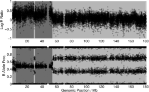
Figure 1: Example: SNP genotyping data. A SNP genotyping data comprises two sets of measurements—the Log R Ratio and the B allele frequency-measured at multiple locations along the genome. Alterations in the distributions of the measurements correspond to underlying changes in the DNA copy number. Each coloured region corresponds to a different underlying DNA copy number state.

With modern high-density microarrays and next generation sequencing data it is possible to reveal many hundreds of structural aberrations within a single tumour. These aberrations can range in size from large, whole or partial chromosomal gains and losses to small focal aberrations affecting potential driver mutations (oncogenes and tumour suppressors). Current state-of-the-art methods can report accurate copy profiles but can lead to practical problems: a collection of lengthy, unmanageable lists of genomic alterations that must be screened by cancer biologists. In this paper, we will show that our decision-theoretic methods can be used to augment existing models and provide increased flexibility for sequence classification. We demonstrate the utility of these methods as a means to report smoother copy number profiles that retain key copy number alterations while having reduced overall complexity.

3 Motivation

3.1 Decision theory

We begin by defining some notation. Let $x_{i}\in\{0,\break\ldots,S\}$ denote the true unobserved underlying state at the $i=1,\ldots,n$ locations, and $y_{i}$ the corresponding observation. The task is to obtain a prediction $\hat{x}=\{\hat{x}_{1},\ldots,\hat{x}_{n}\}$ given a statistical model $\pi(x|y)$ [for notational simplicity, we shall suppress the conditioning on $y$ in the following and refer to $\pi(x|y)$ as $\pi(x)$].

Bayesian decision theory [Berger (1985), Bernardo and Smith (2000)] provides an axiomatic framework for making optimal decisions via the principle of minimum expected loss (or maximum expected utility). In our problem the “decision” is the reporting of $\hat{x}$ from which a set of actions will be taken with associated losses based on the unknown true state of nature $x$. We encapsulate the forms of error into a loss function $l(\hat{x}|x)$ which quantifies the loss of taking actions with $\hat{x}$ when the true state of nature is $x$. The principle of minimum expected loss (MEL) prescribes one should report $\hat{x}$ as

$$\hat{x} = \arg\min_{\tilde{x}}\mathbb{E}_{\pi(x)}\bigl{[}l(\tilde{x}|x)\bigr{]},$$

$$= \arg\min_{\tilde{x}}\sum_{x}l(\tilde{x}|x)\pi(x).$$

3.2 Standard summaries for segmental classification

Two summary predictions that are often used for $\hat{x}$ are as follows: (i) the most probable sequence $\hat{x}=\arg\max_{x}\pi(x)$ (MAP) or (ii) the set of marginally most probable classifications (MaxMarg), $\hat{x}_{i}=\arg\max_{x_{i}}\sum_{x_{-i}}\pi(\{x_{i},x_{-i}\})$ where the summation is over $x_{-i}$, the state sequence other than $x_{i}$. From a decision theoretic perspective, it is interesting to note the corresponding loss functions that would motivate the use of these summaries.

In the case of the MAP sequence, the implicit loss function is the following:

$$l_{G}(\hat{x}|x)=\cases{0,&\quad${\mbox{if }}\hat{x}\equiv x,$\vspace*{2pt}\cr 1,&\quad${\mbox{otherwise}}.$}$$ (1)

We shall refer to this as the global loss function, as a constant penalty is incurred if the prediction is not completely correct. This loss function is extreme in the sense that no matter how many misclassification errors are made, the same penalty is incurred, that is, it is an “all-or-nothing approach.” Furthermore, for this loss function the entirety of the sequence is important, the optimal prediction must be globally and locally correct.

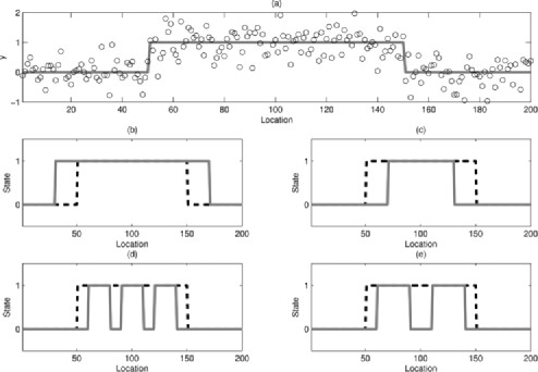
Figure 2: Sequence predictions. An example data set (a) and four predictions of the underlying state sequence (b)–(e). (Grey, solid) Predicted and (Black, dashed) true state sequence.

For the MaxMarg sequence, the implicit loss function assumed is as follows:

$$l(\hat{x}|x)=\sum_{i}l_{M}(\hat{x}_{i}|x_{i}),$$

with

$$l_{M}(\hat{x}_{i}|x_{i})=\cases{0,&\quad${\mbox{if }}\hat{x}_{i}\equiv x_{i},$\vspace*{2pt}\cr\mathrm{FC},&\quad${\mbox{otherwise}},$}$$ (2)

where $\mathrm{FC}$ is the cost of making a false classification. We shall refer to this as the marginal loss function.

In contrast to the global loss function, the marginal loss function ignores any form of local or global structure. It concentrates instead on penalising classification error at each location considered independently of others, which is equivalent to stating that the overall loss is invariant to permutations of the sequence $\{\hat{x}_{i},x_{i}\}_{i=1}^{n}$. As a result, if we consider the simulated data sequence in Figure 2(a) which contains a region of elevated signal related to an underlying change in the hidden state, the predictions shown in Figure 2(b)–(e) which contain the same number of misclassifications may incur the same loss under the marginal loss function even though each prediction is qualitatively very different and may contain a different number of predicted segments that could lead to quite different actions if decisions are taken upon them. It is clear, therefore, that simply counting the number of state misclassifications is insufficient.

3.3 Limitations of standard summaries

These two commonly used loss functions correspond to quite opposite extremes and neither scenario seems appropriate in segmental classification problems. For example, in many situations it is unusual for classification errors to be completely intolerable, instead there are acceptable tolerance levels for error. Under these circumstances it would not be appropriate to use the global loss function in which the same penalty is incurred irrespective of how many errors are made in the prediction. Moreover, there is no flexibility with the global loss and the user cannot explore other predictions with fewer or greater number of transitions. Furthermore, if we are interested in segmental classification and we expect dependencies between states at different locations, it does not seem appropriate to use a marginal loss function that considers classification error at each location independently of the others.

Nonetheless, the appeal of these loss functions is that the computation of the state sequence with minimum expected loss is often analytically tractable or simple to approximate with commonly used statistical models. For example, in Hidden Markov models, the Viterbi algorithm allows the most probable sequence to be enumerated exactly while the forward–backward algorithm allows the marginal probabilities $\pi(x_{i})=\sum_{x_{-i}}\pi(x)$ with computational time complexity that is linear in the length of the data sequence [Rabiner (1989)].

4 Method

4.1 Markov loss function

We now introduce a loss function for segmental classification that penalises incorrect state classifications and transitions:

$$l_{\mathrm{ML}}(\tilde{x}|x)=\sum_{i=1}^{n}l_{M}(\tilde{x}_{i}|x_{i})+\sum_{i=1}^{n-1}l_{T}(\tilde{x}_{i,i+1}|x_{i,i+1}),$$

where $x_{i,i+1}$ denotes the pair $\{x_{i},x_{i+1}\}$. We refer to this as the Markov loss function. This loss function extends the marginal loss function $l_{M}(\tilde{x}|x)$ to include penalty terms on state transition errors $l_{T}(\tilde{x}_{i,i+1}|x_{i,i+1})$ as follows:

$$l_{T}(\tilde{x}_{i,i+1}|x_{i,i+1})=\cases{\mathrm{FT},&\quad$\mbox{if }\tilde{x}_{i}\neq\tilde{x}_{i+1},x_{i}=x_{i+1}$,\vspace*{2pt}\cr\mathrm{FH},&\quad$\mbox{if }\tilde{x}_{i}=\tilde{x}_{i+1},x_{i}\neq x_{i+1},$\vspace*{2pt}\cr 0,&\quad$\mathrm{otherwise},$}$$

where for exposition we assume a common cost of error irrespective of the actual state.

The Markov loss function contains three parameters: (i) $\mathrm{FC}$ (False Call)—cost of a state classification error, (ii) $\mathrm{FT}$ (False Transition)—the cost associated with calling a false state transition and (iii) $\mathrm{FH}$ (False Hold)—the cost of incorrectly staying in the same state. In the special case when $\mathrm{FT}=\mathrm{FH}=0$, the Markov loss function reduces to the marginal loss function which forms a subclass of our more general loss function. An example pairwise loss function for a binary state problem is shown in Table 1.

Table 1: Cost matrix structure for binary state transition

		$\bolds{x}$
$\bolds{l_{\mathrm{\mathbf{ML}}}(\tilde{x}|x)}$		(0, 0)	(0, 1)	(1, 0)	(1, 1)
$\tilde{x}$	(0, 0)	0	$\mathrm{FH}$	$\mathrm{FC+FH}$	$\mathrm{FC}$
	(0, 1)	$\mathrm{FT}$	0	$\mathrm{FC+FT}$	$\mathrm{FC+FT}$
	(1, 0)	$\mathrm{FC+FT}$	$\mathrm{FC+FT}$	0	$\mathrm{FT}$
	(1, 1)	$\mathrm{FC}$	$\mathrm{FC+FH}$	$\mathrm{FH}$	0

4.2 Calculating the expected loss under the Markov loss function

Under the Markov loss function, the expected loss is given by

$$\mathbb{E}_{\pi(x)}\bigl{[}l(\tilde{x}|x)\bigr{]}=\sum_{x}\Biggl{[}\sum_{i=1}^{n}l_{M}(\tilde{x}_{i}|x_{i})+\sum_{i=1}^{n-1}l_{T}(\tilde{x}_{i,i+1}|x_{i,i+1})\Biggr{]}\pi(x),$$

where, by exchanging the order of summation,

$$\mathbb{E}_{\pi(x)}\bigl{[}l(\tilde{x}|x)\bigr{]} = \sum_{i=1}^{n}\sum_{x_{i}}l_{M}(\tilde{x}_{i}|x_{i})\pi(x_{i})+\sum_{i=1}^{n-1}\sum_{x_{i,i+1}}l_{T}(\tilde{x}_{i,i+1}|x_{i,i+1})\pi(x_{i,i+1})$$

$$= \sum_{i=1}^{n}\mathbb{E}_{\pi(x_{i})}\bigl{[}l_{M}(\tilde{x}_{i};x_{i})\bigr{]}+\sum_{i=1}^{n-1}\mathbb{E}_{\pi(x_{i,i+1})}\bigl{[}l_{T}(\tilde{x}_{i,i+1}|x_{i,i+1})\bigr{]},$$

where $\mathbb{E}_{\pi(x_{i})}[l_{M}(\tilde{x}_{i}|x_{i})]$ and $\mathbb{E}_{\pi(x_{i,i+1})}[l_{T}(\tilde{x}_{i,i+1}|x_{i,i+1})]$ are the expected posterior marginal state and switching losses, respectively.

4.3 Dynamic programming

As the expected loss for the Markov loss function is additive, the prediction $\hat{x}$ that has MEL can be found using the following dynamic programming recursions (in similar fashion to the Viterbi algorithm):

4.3.1 Forward recursion

Compute

$$\phi_{1}(k) = \min_{j}\gamma\bigl{(}\tilde{x}_{1,2}=(j,k)\bigr{)},$$

$$\delta_{1}(k) = \arg\min_{j}\gamma\bigl{(}\tilde{x}_{1,2}=(j,k)\bigr{)},$$

where $k\in\{0,\ldots,S\}$, and then for $i=2,\ldots,n$,

$$\phi_{i}(k) = \min_{j}\bigl{[}\phi_{i-1}(j)+\gamma\bigl{(}\tilde{x}_{i,i-1}=(j,k)\bigr{)}\bigr{]},$$

$$\delta_{i}(k) = \arg\min_{j}\bigl{[}\phi_{i-1}(j)+\gamma\bigl{(}\tilde{x}_{i,i-1}=(j,k)\bigr{)}\bigr{]},$$

where $\gamma(\tilde{x}_{i,i-1})=\sum_{x_{i}}l_{M}(\tilde{x}_{i}|x_{i})\pi(x_{i})+\sum_{x_{i,i-1}}l_{T}(\tilde{x}_{i,i-1}|x_{i,i-1})\pi(x_{i,i-1})$.

4.3.2 Backward trace

Find $\hat{x}_{n}=\arg\min_{k}\phi_{n}(k)$, then $\hat{x}_{i-1}=\delta_{i}(\hat{x}_{i}),i=n-1,\ldots,2$.

4.4 Computational requirements

The order of computation required is ${\mathcal{O}}(S^{4}N)$, where $S$ is the number of states and $N$ is the sequence length, since a summation is required over all possible pairs of the true hidden states $x_{i,i+1}$ and predictions $\tilde{x}_{i,i+1}$. This can be prohibitive for applications involving large state spaces but is computationally manageable for smaller state spaces. In practical situations, though, it is often the case that the posterior probability distribution assigns high probabilities to a few transitions while the remainder have negligible probability. For data exhibiting sparse properties, these features can be exploited in order to derive approximate algorithms for inference in Hidden Markov models [see Siddiqi and Moore (2005)] that can offer substantial computational gains at the expense of little error if the assumption of sparseness holds.

4.5 Uncertainty in the statistical model

We have assumed throughout the availability of the exact statistical model $\pi(x|y)$. In general, of course, it is rare in practice to have access to the exact statistical model and instead the model is known up to a form $\pi(x,\theta|y)$ that includes some unknown model parameters $\theta$. The prediction must then satisfy

$$\hat{x} = \arg\min_{\tilde{x}}\int_{\Theta}\biggl{[}\sum_{x\in\mathcal{X}}l(\tilde{x}|x)\pi(x,\theta|y)\biggr{]}\,d\theta$$

$$= \arg\min_{\tilde{x}}\sum_{x\in\mathcal{X}}l(\tilde{x}|x)\pi(x|y)$$

$$\approx \arg\min_{\tilde{x}}\sum_{x\in\mathcal{X}}l(\tilde{x}|x)\hat{\pi}(x|y),$$

where, in the second line, the independence of the loss function and the model parameters allow $\theta$ to be integrated out of the model $\pi(x,\theta|y)$ and the problem is reduced to the same form as before. The integral required will generally be analytically intractable and an estimate $\hat{\pi}(x|y)$ must be used that can be obtained using Monte Carlo simulations, variational methods or by conditioning on point estimators (such as the MAP).

4.5.1 Connections to the discrete Fused Lasso method

Motivated by a similar problem to the one we consider here, Zhang et al. (2010) adopted a dynamic programming imputation method, based on a discrete version of the Fused Lasso prior, to penalise state transitions. The objective function being minimized has the general form

$$\hat{x}=\arg\min_{x}\Biggl{[}\sum_{i=1}^{n}g(x_{i};y,\theta)+\lambda\sum_{i=2}^{n}(1-\delta_{x_{t-1},x_{t}})\Biggr{]},$$

where $g(x_{i};y,\theta)$ is a cost term related to data fidelity, for example, the negative log-likelihood $-\log f(y_{i};x_{i},\theta)$, $\lambda$ is a Lasso penalty for state transitions and $\delta_{x_{i-1},x_{i}}$ is the Kronecker delta function. Note that Zhang et al. (2010) actually penalise the absolute difference in signal level between copy number assignments, but we do not do this here, as, in contrast to the examination of germline copy number alterations, large copy number changes in cancers are frequently occurring.

The Fused Lasso term resembles a one-dimensional stationary Markov Random Field prior of the form $\pi(x)\propto\exp(-\lambda\sum_{i=2}^{n}(1-\delta_{x_{i-1},x_{i}}))$. Since, in one dimension, a stationary Markov Random Field can be expressed as a Markov chain with a particular transition matrix [Kesten (1976)], the method of Zhang et al. (2010) can be equivalently expressed as finding the Viterbi sequence for a Hidden Markov model and the Lasso parameter $\lambda$ provides controls over the prior expected holding times for the Markov chain. In particular, as only a single parameter is used to control the state transition penalties, the transition matrix is symmetric and all states will share the same expected geometric length distribution. Structured nonsymmetric transitions can be specified by transition-specific losses.

An illustration of this relationship can be considered in the symmetric two-state case. The conditional distribution of $X_{i}|X_{i-1},X_{i+1}$ for the Markov Random Field is given by

$$\mathrm{Pr}(X_{i}=x_{i}|X_{i-1}=x_{i-1},X_{i+1}=x_{i+1})$$

$$\qquad=\frac{\exp(-\lambda(1-\delta_{x_{i-1},x_{i}}))\exp(-\lambda(1-\delta_{x_{i},x_{i+1}}))}{\sum_{s=1}^{S}\exp(-\lambda(1-\delta_{x_{i-1},s}))\exp(-\lambda(1-\delta_{s,x_{i+1}}))}.$$

If an equivalent Markov chain exists, with self-transition probability$\mathrm{Pr}(X_{i}=x_{i-1}|X_{i-1}=x_{i-1})=1-\alpha$, the conditional distribution can also be expressed as

$$\mathrm{Pr}(x_{i}|x_{i-1},x_{i+1})=\cases{\displaystyle\frac{\alpha^{2}}{(1-\alpha)^{2}+\alpha^{2}},&\quad$x_{i}\neq x_{i-1},x_{i}\neq x_{i+1}$,\vspace*{2pt}\cr\displaystyle\frac{(1-\alpha)^{2}}{(1-\alpha)^{2}+\alpha^{2}},&\quad$x_{i+1}=x_{i}=x_{i-1}$,\vspace*{2pt}\cr 0.5,&\quad$\mbox{otherwise}.$}$$

By equating these expressions and solving the resulting quadratic, one can obtain the following relationship between the transition probability $\alpha$ and the Fused Lasso penalty $\lambda$:

$$\alpha=\frac{\beta-\sqrt{\beta}}{\beta-1},$$

where $\beta=\exp(-2\lambda)$. Figure 3 shows that for values of $\lambda$ considered by Zhang et al. (2010) ($\lambda=0\mbox{--}10$), the transition probability is accordingly small, which is the desired property for applications in copy number calling applications where DNA copy number state is expected to persist across sizeable genomic regions.

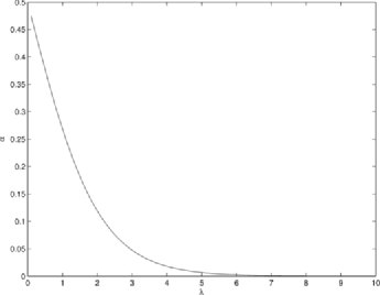
Figure 3: The relationship between the Fused Lasso penalty $\lambda$ and the Markov chain transition probability $\alpha$.

As the discrete Fused Lasso of Zhang et al. (2010) implicitly invokes a structured Hidden Markov model, it therefore can be used as the base model $\pi(x|y)$ for our decision theoretic approach. In addition, there are some interesting connections between the discrete Fused Lasso and our decision theoretic approach. In particular, we can interpret our method as applying a discrete Fused Lasso type reporting process a posteriori rather than a priori. Our method uses the expected posterior marginal site-wise and pair-wise losses from a statistical model that has already been fitted to data. This separation of the reporting and model fitting tasks means that our loss function does not become a proxy for the prior distribution on sequences. This allows a user to modify the sequence classification without having to change the statistical model that is fitted to the data. The benefits of this approach over the Fused Lasso are illustrated and discussed in the following simulation study.

5 Results

5.1 Simulations

We performed a simulation study to examine the properties of predictions made by the use of Viterbi, Fused Lasso and Markov loss functions in a generic segmental classification setup.

5.1.1 Assessing performance

In order to assess performance, we will consider two performance metrics: (i) the site-wise $(\mathrm{e}_{c})$ and (ii) segment-wise $(\mathrm{e}_{s})$ misclassification rates. These are defined as

$$\mathrm{e}_{c}=1-\sum_{i=1}^{N}\delta_{\hat{x}_{i},x_{i}},\qquad\mathrm{e}_{s}=1-\frac{1}{K}\sum_{k=1}^{K}\biggl{[}\frac{1}{|S_{k}|}\sum_{i\in S_{k}}\delta_{\hat{x}_{i},x_{i}}\biggr{]},$$

where $(\hat{x}_{i},x_{i})$ are the prediction and true state at the $i$th position, $K$ is the number of segments in the prediction and $S_{k}$ is the subset of locations spanned by the $k$th segment. A segment-wise misclassification error $e_{s}=0$ means all segments are correctly classified, while $e_{s}=1$ means no segments are found correctly. In this measure, segments contribute equally to the segment-wise performance measure regardless of size. For the motivating application, this is appropriate, as many small genomic aberrations are of greater biological importance than larger structural alterations. The latter, however, contribute more significantly to site-wise classification error.

5.1.2 Simulation models

We simulated data sets, each consisting of 100 data sequences of length $n=1000$ for four different scenarios. The first two data sets were simulated according to a Hidden Markov model with Gaussian observation densities,

$$\pi\bigl{(}y_{i}|x_{i}=k,\mu,\sigma^{2}\bigr{)} = \mathrm{Normal}\bigl{(}\mu_{k},\sigma^{2}\bigr{)},\qquad i=1,\ldots,n,$$

$$\pi(x_{i}=j|x_{i-1}=k) = \Pi_{jk},\qquad i=2,\ldots,n,$$

$$\pi(x_{1}=k) = \nu_{k},\qquad j=1,\ldots,S,$$

with a uniform prior state occupancy vector $\nu$ and the transition matrix $\Pi$ and mean levels $\mu$ are given in Table 2(a), (b).

Table 2: Parameter settings for simulation study

Simulation	Transition matrix, $\bolds{\Pi}$	State durations, $\bolds{\lambda}$	State levels, $\bolds{\mu}$
(a) HMM (Sticky)	$\left[\matrix{9/10&1/30&1/30&1/30\vspace*{2pt}\cr 1/30&9/10&1/30&1/30\vspace*{2pt}\cr 1/30&1/30&9/10&1/30\vspace*{2pt}\cr 1/30&1/30&1/30&9/10}\right]$	n/a	$\{-1,0,1,2\}$
(b) HMM (Dynamic)	$\left[\matrix{0.5&0.2&0.2&0.1\vspace*{2pt}\cr 0.4&0.6&0.0&0.0\vspace*{2pt}\cr 0.0&0.1&0.7&0.2\vspace*{2pt}\cr 0.2&0.0&0.0&0.5}\right]$	n/a	$\{-1,0,1,2\}$
(c) HSMM (4-state)	$\left[\matrix{0.0&0.2&0.5&0.3\vspace*{2pt}\cr 0.2&0.0&0.5&0.3\vspace*{2pt}\cr 0.1&0.3&0.0&0.6\vspace*{2pt}\cr 0.2&0.4&0.4&0.0}\right]$	$\{20,50,20,10\}$	$\{-1,0,1,2\}$
(d) HSMM (5-state)	$\left[\matrix{0.0&0.25&0.25&0.25&0.25\vspace*{2pt}\cr 0.25&0.0&0.25&0.25&0.25\vspace*{2pt}\cr 0.25&0.25&0.0&0.25&0.25\vspace*{2pt}\cr 0.25&0.25&0.25&0.0&0.25\vspace*{2pt}\cr 0.25&0.25&0.25&0.25&0.0}\right]$	$\{30,50,30,20,10\}$	$\{-1,0,1,2,5\}$

The third and fourth data sets were generated according to Hidden Semi-Markov model sequences via the following scheme:

$$y_{t}|z_{t}=s,\qquad\sigma^{2} \sim \mathrm{Normal}\bigl{(}\mu_{s},\sigma^{2}\bigr{)},$$

$$z_{t+1:t+\Delta_{i}} = x_{i},t=\sum_{j=1}^{i-1}\Delta_{j},$$

$$\Delta_{i}|x_{i}=k,\qquad\lambda \sim \mathrm{Poisson}(\lambda_{k}),\qquad i=2,\ldots,N,$$

$$p(x_{i}=j|x_{i-1}=k) = \Pi_{jk},\qquad i=2,\ldots,N,(j,k)\in\{1,\ldots,S\}^{2}$$

$$p(x_{1}=j) = \nu_{j},\qquad j=1,\ldots,S,$$

where the transition matrix $\Pi$, state durations $\lambda$ and mean levels $\mu$ are shown in Table 2(c), (d).

5.1.3 Statistical inference

We fitted a Hidden Markov model with Gaussian observation densities to each data sequence. We assumed that the parameters of the observational density $(\mu,\sigma^{2})$ are given, but we used a standard expectation-maximization (or Baum–Welch algorithm) to obtain maximum likelihood parameter estimates for the prior state occupancy vector $\hat{\nu}$ and transition matrix, $\hat{\Pi}$. Note that our primary interest here is the methods for reporting sequence predictions and not the model fitting procedures themselves which we consider a separate exercise. Given the parameter estimates, we applied three methods for segmental classification: (i) we used the Viterbi algorithm to find the most probable state sequence $\hat{x}_{v}$; (ii) the discrete Fused Lasso method with a range of penalty values $\lambda=1\mbox{--}10\mbox{,}000$; and, finally, (iii) we applied the forward–backward algorithm to obtain the marginal state and switching probabilities $\pi(x_{i}|y)$ and $\pi(x_{i,i+1}|y)$ and applied our decision-theoretic approach with loss parameter values $\mathrm{FC}=1$, $\mathrm{FN}=1$ and a range $\mathrm{FT}=1\mbox{--}10\mbox{,}000$.

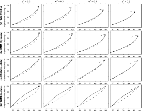
Figure 4: Classification of simulated Markov and Semi-Markov sequences under first-order Markov assumptions. $(-)$ Markov loss. $(--)$ Fused Lasso. $(\times)$ Viterbi.

5.1.4 Results

Figure 4 shows the average performance of the three segmentation methods on the four data sets. The Viterbi segmentation gives excellent site-wise and segment-wise classification accuracy in all cases. Similar classification performance may be achieved using the Fused Lasso for a certain choice of penalty parameter $\lambda$. This parameter would need to be learnt in real applications. For our decision-theoretic approach, Viterbi-like performance can be achieved using a default choice of unit loss parameters $\mathrm{FC}=\mathrm{FH}=\mathrm{FT}=1$ which is convenient for default analyses.

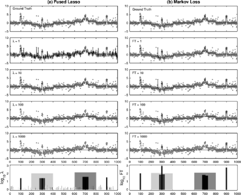
Figure 5: Example segmentations using the Fused Lasso and Markov loss functions for different transition penalties.

We remark that the Viterbi and Fused Lasso solutions are only available as we condition on fixed or point parameter estimates. In a full Bayesian analysis, where Markov chain Monte Carlo (MCMC) methods are used to sample from the joint posterior distribution, these solutions would not be available. However, our decision-theoretic approach can utilise Monte Carlo approximations of the posterior expected marginal losses and can be applied to MCMC output.

Our principle interest, though, is not the single prediction provided by Viterbi but the Fused Lasso and our proposed decision-theoretic approach for exploring alternative segmentations. In this case, by increasing the transition penalties ($\lambda$ and $\mathrm{FT}$, resp.), each method is able to produce less complex (smoother) segmentations with fewer segments. However, Figure 4 shows that for a given site-wise classification accuracy, our decision-theoretic approach is able to attain a higher segment-wise classification accuracy than the Fused Lasso method.

Figure 5 explains the differing segmentation behaviours. As shown previously, the Fused Lasso penalty $\lambda$ is related to the prior expected segment length, and large values of $\lambda$ imply a preference for larger (and therefore fewer) segments. As a consequence, the short segments tend to be the first to be eliminated from the Fused Lasso segmentations, while larger segments are retained. This is because the contribution of small segments to the overall sequence likelihood is insufficient to justify the penalty of having two breakpoints to define the small segment.

With our decision-theoretic approach, when computing the expected loss, the loss penalties are scaled by the posterior marginal site-wise and transition probabilities. Hence, as the penalty on false transitions $(\mathrm{FT})$ is increased, it is those breakpoints that are associated with low probability state transitions which are eliminated first. The segmentations that are produced using the Markov loss function therefore show a reduction in complexity as the transition loss $\mathrm{FT}$ is increased, but retain the short, high signal segments in the data sequence with high probability breakpoints. We shall see the practical implications of this in the following application study.

5.2 Application: DNA copy number profiling of colorectal cancer

5.2.1 Setup

We now consider the use of our methods as an augmented step in existing Hidden Markov model based approaches for classifying DNA copy number alterations. One of the problems with such a task is the difficulty of making formal performance assessments due to a unavailability of “gold standard” genome-wide copy number profiles for cancers. Standard experimental approaches, such as FISH or PCR, lack the resolution and throughput necessary to confirm the hundreds to thousands of possible findings arising from more modern technologies based on microarrays of next generation sequencing technologies. As a consequence, in the absence of ground truth data, we adopted the following simulation set up to produce realistic data sets for evaluation.

We collated a genome-wide DNA copy number data set derived from a recent study of colorectal cancers [Christie et al. (2012)] consisting of over 630 colorectal tumours. Secondly, for each tumour, the raw microarray data was processed using a state-of-the-art method, OncoSNP [Yau et al. (2010)], to infer the DNA copy number profile. Finally, from this collection of tumour copy number profiles, we then simulated a series of one-dimensional data sets with Student $t$-distributed noise using these copy number profiles as a scaffold. The simulation strategy is illustrated graphically in Figure 6 using a data set derived from a colorectal tumour exhibiting chromosomal instability—a common phenomenon in colorectal cancers. Chromosomal instability gives rise to large segments with shorter segments interspersed along the genome residing at sites containing genes with potential oncogenic or tumor suppressing activity.

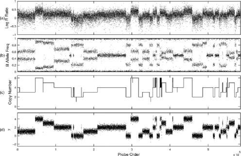
Figure 6: Cancer simulation strategy. (a), (b) SNP data from the original colorectal tumor was analysed using OncoSNP [Yau et al. (2010)] to obtain a copy number profile (c). Using this copy number profile we simulated a new data set (d) upon which we tested the Viterbi, Fused Lasso and our decision-theoretic approaches for segmental classification.

This strategy allows us to generate copy number sequence data with real-world characteristics where we know the truth, and hence better understand the effect of using Viterbi, the Fused Lasso and our preferred method based on Markov loss functions for segmental classification. This partially circumvents the lack of “gold standard” copy number profiles for complex tumour samples, without which we are not able to verify the accuracy of the copy number profile predictions that would be inferred.

5.2.2 Simulations

Given a DNA copy number profile $x_{1},\ldots,x_{N}$ involving $S$ copy number states, we simulated a data set $y$ according to the following scheme:

$$y_{i}|x_{i}=k,\qquad\sigma^{2}\sim\mathrm{Student}\bigl{(}\mu_{k},\sigma^{2},\nu\bigr{)},\qquad i=1,\ldots,N,$$ (3)

where $\nu=4$ and $\mu=\log(k/2)$ and $\mu=-4$ for $k=0$ in the simulations (our simulations mimic the nonlinear response behaviour of homozygous deletions that involve zero copy number in microarray experiments). As before, we fitted a Hidden Markov model to the data using the EM algorithm to obtain maximum likelihood estimates of the initial state occupancy vector and transition matrix. We applied the Viterbi algorithm, Fused Lasso and our decision-theoretic method to give a segmental classification of the data compared to the actual profile used to generate the data sequence.

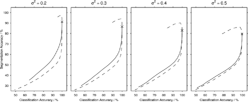
Figure 7: Classification performance on the colon cancer data set. $(-)$ Markov loss. $(--)$ Fused Lasso. $(\times)$ Viterbi.

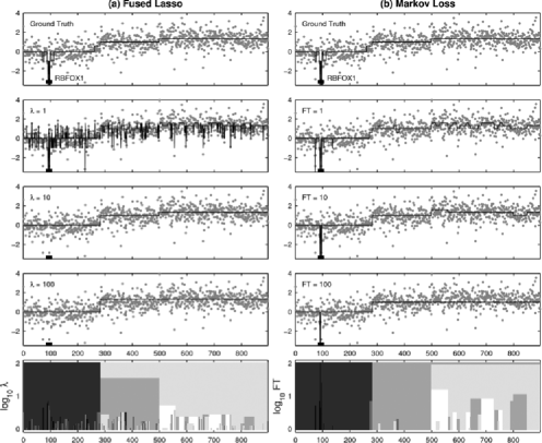
Figure 8: Example segmentations using the Fused Lasso and Markov loss functions for a tumour containing an RBFOX1 deletion.

Note, for these applications, a true physical basis for the statistical model $\pi(x)$ is unknown and first-order Markov models are often used as an approximation. Semi-Markov models provide greater modeling flexibility but are rarely used in genomic applications, as the data sets involve long sequences (in our CRC application $N=6\times 10^{5}$). Inference methods for the semi-Markov models have computational requirements that are order ${\mathcal{O}}(S^{2}N^{2})$ [Murphy (2002)], which preclude their use in real applications.

5.2.3 Results

Figure 7 shows that using the Markov loss function we were able to achieve improved segmental classification rates compared to the Fused Lasso for the colon cancer data set. A specific example is illustrated in Figure 8 which shows data simulated based on a tumour carrying a number of large copy number alterations on chromosome 16 and a small homozygous deletion involving the alternative splicing factor RBFOX1. Deletions of RBFOX1 are a recurrent event in colorectal cancer [Cancer Genome Atlas Network (2012)] and were recently found to have high prevalence in patients from a Bangladeshi population versus Caucasians [Sengupta et al. (2013)]. Deletions in this region are complex, with focal deletions targeting the 5^′ end of the gene, and have been shown to affect mRNA and protein expression in colorectal cell lines and tumours. A copy number profile of this tumour should ideally report the presence of the RBFOX1 deletion, but the other larger copy number changes may be of less importance as they are likely to be passenger events formed due to genomic instability during tumour evolution.

In the Fused Lasso segmentations, we can encourage smoother segmentations by increasing the transition penalty. However, the effect of using larger penalties causes the important RBFOX1 deletion to be eliminated and only the larger copy number alterations are retained. With our decision-theoretic approach, the RBFOX1 deletion is identified even when the false transition loss parameter was increased—we are able to achieve smoothing without losing this important fine detail.

These results indicate that our method could be used to augment existing Hidden Markov model-based calling algorithms for copy number aberrations, such as those by Sun et al. (2009), Yau et al. (2010) and Li et al. (2011), with a sequence classification algorithm that provides a more flexible alternative to the Viterbi algorithm and has improved segmental classification performance relative to the Fused Lasso method. In particular, we demonstrate the adaptive nature of the Markov loss function, in terms of its ability to provide reduced complexity copy number segmentations while retaining important features such as small homozygous deletions or gene amplifications. This may assist cancer researchers in isolating important genetic alterations of interest in cases where a default Viterbi segmentation might produce unmanageably complex copy profiles.

6 Discussion

Segmental classification problems are ubiquitous across many fields, including signal processing, finance and, more recently, genomics. We have introduced a Markov loss function that allows a user to take their preferred statistical model $\pi(x)$ of the sequence $x$ and obtain a sequence prediction $\hat{x}$ whose properties can be adjusted in an intuitive way by specifying loss parameters on state and transition errors. The calculation of the posterior expected loss with respect to a Markov loss function was shown to have a simple form and a dynamic programming algorithm was provided to compute the state sequence with the minimum expected loss.

Although the emphasis in this presentation was on the Hidden Markov model as the statistical model $\pi(x)$, this method can be applied to any statistical model for the segmentation and classification of linear sequence data that can provide estimates of the marginal state transition probability $\pi(x_{i,i+1})$. Therefore, it can be used to augment, without modification, many existing statistical methods for analyzing sequence data, such as those based on semi-Markov models, change point methods [Fearnhead and Liu (2007)] or product partition models [Barry and Hartigan (1992)]. While it is a relatively simple addition, the application of this method could greatly enhance the adaptability of many existing statistical algorithms, transferring power to the experimenter to allow them to assign losses to various error types relevant to their own study.

Our approach can be considered to be a specific form of the loss functions considered by Rue (1995) in Bayesian imaging applications. Rue (1995) considered a more complex two-dimensional domain, using Markov Random Field priors, where exact enumeration of the optimal decision is impossible and numerical optimisation using computationally-intensive MCMC and simulated annealing is required. Recently, Lember and Koloydenko (2010) have also considered generalised risk-based inference for Hidden Markov models including a subclass of posterior decoding schemes that can be viewed as hybrids of the Viterbi and marginal approaches.

Throughout this paper we have not explicitly stated how the loss values should be selected. This is purposeful because the selection of the costs associated with various error types is study-dependent and the individual data analyst must balance the appropriate losses for the particular application. For example, in genomics, costs might be related to tangible quantities such as the financial, time and manpower requirements for follow-up studies and validation taken upon the predictions. We indicate that a default choice of loss parameters can lead to a Viterbi-like performance.

It is also of further research interest to characterise the effect on predictions when only an approximation of the statistical model is available. Furthermore, in some applications there may be some utility in combining of Markov loss functions on the hidden state sequence $x$ and loss functions on the model parameters $\theta$. The Markov loss function introduced here focuses on costs associated with classification errors of the hidden state sequence and assumes that the model parameters are in some sense nuisance variables. There are applications where both the state sequence and model parameters may be of interest; for example, the transition matrix may have some interpretation for a given application and a loss function may be given on $\theta$. In these instances it may be necessary to derive optimal joint predictions $(\hat{x},\hat{\theta})$ under the appropriate loss functions.

References

- Banachewicz, Lucas and van der Vaart (2008) {barticle}[author] \bauthor\bsnmBanachewicz, \bfnmK.\binitsK., \bauthor\bsnmLucas, \bfnmA.\binitsA. and \bauthor\bparticlevan der \bsnmVaart, \bfnmA.\binitsA. (\byear2008). \btitleModelling portfolio defaults using Hidden Markov models with covariates. \bjournalEconom. J. \bvolume11 \bpages155–171. \bptokimsref \endbibitem
- Barry and Hartigan (1992) {barticle}[mr] \bauthor\bsnmBarry, \bfnmDaniel\binitsD. and \bauthor\bsnmHartigan, \bfnmJ. A.\binitsJ. A. (\byear1992). \btitleProduct partition models for change point problems. \bjournalAnn. Statist. \bvolume20 \bpages260–279. \biddoi=10.1214/aos/1176348521, issn=0090-5364, mr=1150343 \bptokimsref \endbibitem
- Berger (1985) {bbook}[mr] \bauthor\bsnmBerger, \bfnmJames O.\binitsJ. O. (\byear1985). \btitleStatistical Decision Theory and Bayesian Analysis, \bedition2nd ed. \bpublisherSpringer, \blocationNew York. \bidmr=0804611 \bptokimsref \endbibitem
- Bernardo and Smith (2000) {bbook}[author] \bauthor\bsnmBernardo, \bfnmJ. M.\binitsJ. M. and \bauthor\bsnmSmith, \bfnmA. F. M.\binitsA. F. M. (\byear2000). \btitleBayesian Theory. \bpublisherWiley, \blocationNew York. \bptokimsref \endbibitem
- Beroukhim et al. (2010) {barticle}[author] \bauthor\bsnmBeroukhim, \bfnmRameen\binitsR., \bauthor\bsnmMermel, \bfnmCraig H.\binitsC. H., \bauthor\bsnmPorter, \bfnmDale\binitsD., \bauthor\bsnmWei, \bfnmGuo\binitsG., \bauthor\bsnmRaychaudhuri, \bfnmSoumya\binitsS., \bauthor\bsnmDonovan, \bfnmJerry\binitsJ., \bauthor\bsnmBarretina, \bfnmJordi\binitsJ., \bauthor\bsnmBoehm, \bfnmJesse S.\binitsJ. S., \bauthor\bsnmDobson, \bfnmJennifer\binitsJ., \bauthor\bsnmUrashima, \bfnmMitsuyoshi\binitsM., \bauthor\bsnmHenry, \bfnmKevin T. Mc\binitsK. T. M., \bauthor\bsnmPinchback, \bfnmReid M.\binitsR. M., \bauthor\bsnmLigon, \bfnmAzra H.\binitsA. H., \bauthor\bsnmCho, \bfnmYoon-Jae\binitsY.-J., \bauthor\bsnmHaery, \bfnmLeila\binitsL., \bauthor\bsnmGreulich, \bfnmHeidi\binitsH., \bauthor\bsnmReich, \bfnmMichael\binitsM., \bauthor\bsnmWinckler, \bfnmWendy\binitsW., \bauthor\bsnmLawrence, \bfnmMichael S.\binitsM. S., \bauthor\bsnmWeir, \bfnmBarbara A.\binitsB. A., \bauthor\bsnmTanaka, \bfnmKumiko E.\binitsK. E., \bauthor\bsnmChiang, \bfnmDerek Y.\binitsD. Y., \bauthor\bsnmBass, \bfnmAdam J.\binitsA. J., \bauthor\bsnmLoo, \bfnmAlice\binitsA., \bauthor\bsnmHoffman, \bfnmCarter\binitsC., \bauthor\bsnmPrensner, \bfnmJohn\binitsJ., \bauthor\bsnmLiefeld, \bfnmTed\binitsT., \bauthor\bsnmGao, \bfnmQing\binitsQ., \bauthor\bsnmYecies, \bfnmDerek\binitsD., \bauthor\bsnmSignoretti, \bfnmSabina\binitsS., \bauthor\bsnmMaher, \bfnmElizabeth\binitsE., \bauthor\bsnmKaye, \bfnmFrederic J.\binitsF. J., \bauthor\bsnmSasaki, \bfnmHidefumi\binitsH., \bauthor\bsnmTepper, \bfnmJoel E.\binitsJ. E., \bauthor\bsnmFletcher, \bfnmJonathan A.\binitsJ. A., \bauthor\bsnmTabernero, \bfnmJosep\binitsJ., \bauthor\bsnmBaselga, \bfnmJosé\binitsJ., \bauthor\bsnmTsao, \bfnmMing-Sound\binitsM.-S., \bauthor\bsnmDemichelis, \bfnmFrancesca\binitsF., \bauthor\bsnmRubin, \bfnmMark A.\binitsM. A., \bauthor\bsnmJanne, \bfnmPasi A.\binitsP. A., \bauthor\bsnmDaly, \bfnmMark J.\binitsM. J., \bauthor\bsnmNucera, \bfnmCarmelo\binitsC., \bauthor\bsnmLevine, \bfnmRoss L.\binitsR. L., \bauthor\bsnmEbert, \bfnmBenjamin L.\binitsB. L., \bauthor\bsnmGabriel, \bfnmStacey\binitsS., \bauthor\bsnmRustgi, \bfnmAnil K.\binitsA. K., \bauthor\bsnmAntonescu, \bfnmCristina R.\binitsC. R., \bauthor\bsnmLadanyi, \bfnmMarc\binitsM., \bauthor\bsnmLetai, \bfnmAnthony\binitsA., \bauthor\bsnmGarraway, \bfnmLevi A.\binitsL. A., \bauthor\bsnmLoda, \bfnmMassimo\binitsM. and \bauthor\bsnmBeer, \bfnmDavid G.\binitsD. G. (\byear2010). \btitleThe landscape of somatic copy-number alteration across human cancers. \bjournalNature \bvolume463 \bpages899–905. \bptokimsref \endbibitem
- Bignell et al. (2010) {barticle}[author] \bauthor\bsnmBignell, \bfnmGraham R.\binitsG. R., \bauthor\bsnmGreenman, \bfnmChris D.\binitsC. D., \bauthor\bsnmDavies, \bfnmHelen\binitsH., \bauthor\bsnmButler, \bfnmAdam P.\binitsA. P., \bauthor\bsnmEdkins, \bfnmSarah\binitsS., \bauthor\bsnmAndrews, \bfnmJenny M.\binitsJ. M., \bauthor\bsnmBuck, \bfnmGemma\binitsG., \bauthor\bsnmChen, \bfnmLina\binitsL., \bauthor\bsnmBeare, \bfnmDavid\binitsD., \bauthor\bsnmLatimer, \bfnmCalli\binitsC., \bauthor\bsnmWidaa, \bfnmSara\binitsS., \bauthor\bsnmHinton, \bfnmJonathon\binitsJ., \bauthor\bsnmFahey, \bfnmCiara\binitsC., \bauthor\bsnmFu, \bfnmBeiyuan\binitsB., \bauthor\bsnmSwamy, \bfnmSajani\binitsS., \bauthor\bsnmDalgliesh, \bfnmGillian L.\binitsG. L., \bauthor\bsnmTeh, \bfnmBin T.\binitsB. T., \bauthor\bsnmDeloukas, \bfnmPanos\binitsP., \bauthor\bsnmYang, \bfnmFengtang\binitsF., \bauthor\bsnmCampbell, \bfnmPeter J.\binitsP. J., \bauthor\bsnmFutreal, \bfnmP. Andrew\binitsP. A. and \bauthor\bsnmStratton, \bfnmMichael R.\binitsM. R. (\byear2010). \btitleSignatures of mutation and selection in the cancer genome. \bjournalNature \bvolume463 \bpages893–898. \bptokimsref \endbibitem
- Cancer Genome Atlas Network (2012) {bmisc}[pbm] \borganizationCancer Genome Atlas Network (\byear2012). \bhowpublishedComprehensive molecular characterization of human colon and rectal cancer. Nature 487 330–337. \biddoi=10.1038/nature11252, issn=1476-4687, mid=NIHMS379461, pii=nature11252, pmcid=3401966, pmid=22810696 \bptokimsref \endbibitem
- Carter et al. (2012) {barticle}[author] \bauthor\bsnmCarter, \bfnmScott L.\binitsS. L., \bauthor\bsnmCibulskis, \bfnmKristian\binitsK., \bauthor\bsnmHelman, \bfnmElena\binitsE., \bauthor\bsnmMcKenna, \bfnmAaron\binitsA., \bauthor\bsnmShen, \bfnmHui\binitsH., \bauthor\bsnmZack, \bfnmTravis\binitsT., \bauthor\bsnmLaird, \bfnmPeter W.\binitsP. W., \bauthor\bsnmOnofrio, \bfnmRobert C.\binitsR. C., \bauthor\bsnmWinckler, \bfnmWendy\binitsW., \bauthor\bsnmWeir, \bfnmBarbara A.\binitsB. A., \bauthor\bsnmBeroukhim, \bfnmRameen\binitsR., \bauthor\bsnmPellman, \bfnmDavid\binitsD., \bauthor\bsnmLevine, \bfnmDouglas A.\binitsD. A., \bauthor\bsnmLander, \bfnmEric S.\binitsE. S., \bauthor\bsnmMeyerson, \bfnmMatthew\binitsM. and \bauthor\bsnmGetz, \bfnmGad\binitsG. (\byear2012). \btitleAbsolute quantification of somatic DNA alterations in human cancer. \bjournalNat. Biotechnol. \bvolume30 \bpages413–421. \bptokimsref \endbibitem
- Chien and Furui (2005) {barticle}[author] \bauthor\bsnmChien, \bfnmJ. T.\binitsJ. T. and \bauthor\bsnmFurui, \bfnmS.\binitsS. (\byear2005). \btitlePredictive hidden Markov model selection for speech recognition. \bjournalIEEE Transactions on Speech and Audio Processing \bvolume13 \bpages377–387. \bptokimsref \endbibitem
- Chopin and Pelgrin (2004) {barticle}[mr] \bauthor\bsnmChopin, \bfnmNicolas\binitsN. and \bauthor\bsnmPelgrin, \bfnmFlorian\binitsF. (\byear2004). \btitleBayesian inference and state number determination for hidden Markov models: An application to the information content of the yield curve about inflation. \bjournalJ. Econometrics \bvolume123 \bpages327–344. \biddoi=10.1016/j.jeconom.2003.12.010, issn=0304-4076, mr=2100417 \bptokimsref \endbibitem
- Christie et al. (2012) {barticle}[author] \bauthor\bsnmChristie, \bfnmM.\binitsM., \bauthor\bsnmJorissen, \bfnmR. N.\binitsR. N., \bauthor\bsnmMouradov, \bfnmD.\binitsD., \bauthor\bsnmSakthianandeswaren, \bfnmA.\binitsA., \bauthor\bsnmLi, \bfnmS.\binitsS., \bauthor\bsnmDay, \bfnmF.\binitsF., \bauthor\bsnmTsui, \bfnmC.\binitsC., \bauthor\bsnmLipton, \bfnmL.\binitsL., \bauthor\bsnmDesai, \bfnmJ.\binitsJ., \bauthor\bsnmJones, \bfnmI. T.\binitsI. T., \bauthor\bsnmMcLaughlin, \bfnmS.\binitsS., \bauthor\bsnmWard, \bfnmR. L.\binitsR. L., \bauthor\bsnmHawkins, \bfnmN. J.\binitsN. J., \bauthor\bsnmRuszkiewicz, \bfnmA. R.\binitsA. R., \bauthor\bsnmMoore, \bfnmJ.\binitsJ., \bauthor\bsnmBurgess, \bfnmA. W.\binitsA. W., \bauthor\bsnmBusam, \bfnmD.\binitsD., \bauthor\bsnmZhao, \bfnmQ.\binitsQ., \bauthor\bsnmStrausberg, \bfnmR. L.\binitsR. L., \bauthor\bsnmSimpson, \bfnmA. J.\binitsA. J., \bauthor\bsnmTomlinson, \bfnmI. P M\binitsI. P. M., \bauthor\bsnmGibbs, \bfnmP.\binitsP. and \bauthor\bsnmSieber, \bfnmO. M.\binitsO. M. (\byear2012). \btitleDifferent APC genotypes in proximal and distal sporadic colorectal cancers suggest distinct WNT/-catenin signalling thresholds for tumourigenesis. \bjournalOncogene. \bnoteDOI:\doiurl10.1038/onc.2012.486. \bptokimsref \endbibitem
- Curtis et al. (2012) {barticle}[author] \bauthor\bsnmCurtis, \bfnmChristina\binitsC., \bauthor\bsnmShah, \bfnmSohrab P.\binitsS. P., \bauthor\bsnmChin, \bfnmSuet-Feung\binitsS.-F., \bauthor\bsnmTurashvili, \bfnmGulisa\binitsG., \bauthor\bsnmRueda, \bfnmOscar M.\binitsO. M., \bauthor\bsnmDunning, \bfnmMark J.\binitsM. J., \bauthor\bsnmSpeed, \bfnmDoug\binitsD., \bauthor\bsnmLynch, \bfnmAndy G.\binitsA. G., \bauthor\bsnmSamarajiwa, \bfnmShamith\binitsS., \bauthor\bsnmYuan, \bfnmYinyin\binitsY., \bauthor\bsnmGräf, \bfnmStefan\binitsS., \bauthor\bsnmHa, \bfnmGavin\binitsG., \bauthor\bsnmHaffari, \bfnmGholamreza\binitsG., \bauthor\bsnmBashashati, \bfnmAli\binitsA., \bauthor\bsnmRussell, \bfnmRoslin\binitsR., \bauthor\bsnmMcKinney, \bfnmSteven\binitsS., \bauthor\bsnmGroup, \bfnmM. E. T. A. B. R. I. C.\binitsM. E. T. A. B. R. I. C., \bauthor\bsnmLangerød, \bfnmAnita\binitsA., \bauthor\bsnmGreen, \bfnmAndrew\binitsA., \bauthor\bsnmProvenzano, \bfnmElena\binitsE., \bauthor\bsnmWishart, \bfnmGordon\binitsG., \bauthor\bsnmPinder, \bfnmSarah\binitsS., \bauthor\bsnmWatson, \bfnmPeter\binitsP., \bauthor\bsnmMarkowetz, \bfnmFlorian\binitsF., \bauthor\bsnmMurphy, \bfnmLeigh\binitsL., \bauthor\bsnmEllis, \bfnmIan\binitsI., \bauthor\bsnmPurushotham, \bfnmArnie\binitsA., \bauthor\bsnmBørresen-Dale, \bfnmAnne-Lise\binitsA.-L., \bauthor\bsnmBrenton, \bfnmJames D.\binitsJ. D., \bauthor\bsnmTavaré, \bfnmSimon\binitsS., \bauthor\bsnmCaldas, \bfnmCarlos\binitsC. and \bauthor\bsnmAparicio, \bfnmSamuel\binitsS. (\byear2012). \btitleThe genomic and transcriptomic architecture of 2000 breast tumours reveals novel subgroups. \bjournalNature \bvolume486 \bpages346–352. \bptokimsref \endbibitem
- Day et al. (2007) {barticle}[pbm] \bauthor\bsnmDay, \bfnmNathan\binitsN., \bauthor\bsnmHemmaplardh, \bfnmAndrew\binitsA., \bauthor\bsnmThurman, \bfnmRobert E.\binitsR. E., \bauthor\bsnmStamatoyannopoulos, \bfnmJohn A.\binitsJ. A. and \bauthor\bsnmNoble, \bfnmWilliam S.\binitsW. S. (\byear2007). \btitleUnsupervised segmentation of continuous genomic data. \bjournalBioinformatics \bvolume23 \bpages1424–1426. \biddoi=10.1093/bioinformatics/btm096, issn=1367-4811, pii=btm096, pmid=17384021 \bptokimsref \endbibitem
- Fearnhead and Liu (2007) {barticle}[mr] \bauthor\bsnmFearnhead, \bfnmPaul\binitsP. and \bauthor\bsnmLiu, \bfnmZhen\binitsZ. (\byear2007). \btitleOn-line inference for multiple changepoint problems. \bjournalJ. R. Stat. Soc. Ser. B Stat. Methodol. \bvolume69 \bpages589–605. \biddoi=10.1111/j.1467-9868.2007.00601.x, issn=1369-7412, mr=2370070 \bptokimsref \endbibitem
- Giampieri, Davis and Crowder (2005) {barticle}[mr] \bauthor\bsnmGiampieri, \bfnmGiacomo\binitsG., \bauthor\bsnmDavis, \bfnmMark\binitsM. and \bauthor\bsnmCrowder, \bfnmMartin\binitsM. (\byear2005). \btitleAnalysis of default data using hidden Markov models. \bjournalQuant. Finance \bvolume5 \bpages27–34. \biddoi=10.1080/14697680500039951, issn=1469-7688, mr=2241629 \bptokimsref \endbibitem
- Greenman et al. (2010) {barticle}[pbm] \bauthor\bsnmGreenman, \bfnmChris D.\binitsC. D., \bauthor\bsnmBignell, \bfnmGraham\binitsG., \bauthor\bsnmButler, \bfnmAdam\binitsA., \bauthor\bsnmEdkins, \bfnmSarah\binitsS., \bauthor\bsnmHinton, \bfnmJon\binitsJ., \bauthor\bsnmBeare, \bfnmDave\binitsD., \bauthor\bsnmSwamy, \bfnmSajani\binitsS., \bauthor\bsnmSantarius, \bfnmThomas\binitsT., \bauthor\bsnmChen, \bfnmLina\binitsL., \bauthor\bsnmWidaa, \bfnmSara\binitsS., \bauthor\bsnmFutreal, \bfnmP. Andy\binitsP. A. and \bauthor\bsnmStratton, \bfnmMichael R.\binitsM. R. (\byear2010). \btitlePICNIC: An algorithm to predict absolute allelic copy number variation with microarray cancer data. \bjournalBiostatistics \bvolume11 \bpages164–175. \biddoi=10.1093/biostatistics/kxp045, issn=1468-4357, pii=kxp045, pmcid=2800165, pmid=19837654 \bptokimsref \endbibitem
- Kesten (1976) {barticle}[mr] \bauthor\bsnmKesten, \bfnmHarry\binitsH. (\byear1976). \btitleExistence and uniqueness of countable one-dimensional Markov random fields. \bjournalAnn. Probab. \bvolume4 \bpages557–569. \bidmr=0410930 \bptokimsref \endbibitem
- Knight et al. (2012) {barticle}[author] \bauthor\bsnmKnight, \bfnmS. J. L.\binitsS. J. L., \bauthor\bsnmYau, \bfnmC.\binitsC., \bauthor\bsnmClifford, \bfnmR.\binitsR., \bauthor\bsnmTimbs, \bfnmA. T.\binitsA. T., \bauthor\bsnmSadighi Akha, \bfnmE.\binitsE., \bauthor\bsnmDréau, \bfnmH. M.\binitsH. M., \bauthor\bsnmBurns, \bfnmA.\binitsA., \bauthor\bsnmCiria, \bfnmC.\binitsC., \bauthor\bsnmOscier, \bfnmD. G.\binitsD. G., \bauthor\bsnmPettitt, \bfnmA. R.\binitsA. R., \bauthor\bsnmDutton, \bfnmS.\binitsS., \bauthor\bsnmHolmes, \bfnmC. C.\binitsC. C., \bauthor\bsnmTaylor, \bfnmJ.\binitsJ., \bauthor\bsnmCazier, \bfnmJ.-B.\binitsJ.-B. and \bauthor\bsnmSchuh, \bfnmA.\binitsA. (\byear2012). \btitleQuantification of subclonal distributions of recurrent genomic aberrations in paired pre-treatment and relapse samples from patients with B-cell chronic lymphocytic leukemia. \bjournalLeukemia \bvolume26 \bpages1564–1575. \bptokimsref \endbibitem
- Lember and Koloydenko (2010) {bmisc}[author] \bauthor\bsnmLember, \bfnmJüri\binitsJ. and \bauthor\bsnmKoloydenko, \bfnmAlexey A\binitsA. A. (\byear2010). \bhowpublishedA generalized risk approach to path inference based on hidden Markov models. Preprint. Available at \arxivurlarXiv:1007.3622. \bptokimsref \endbibitem
- Li et al. (2011) {barticle}[pbm] \bauthor\bsnmLi, \bfnmAo\binitsA., \bauthor\bsnmLiu, \bfnmZongzhi\binitsZ., \bauthor\bsnmLezon-Geyda, \bfnmKimberly\binitsK., \bauthor\bsnmSarkar, \bfnmSudipa\binitsS., \bauthor\bsnmLannin, \bfnmDonald\binitsD., \bauthor\bsnmSchulz, \bfnmVincent\binitsV., \bauthor\bsnmKrop, \bfnmIan\binitsI., \bauthor\bsnmWiner, \bfnmEric\binitsE., \bauthor\bsnmHarris, \bfnmLyndsay\binitsL. and \bauthor\bsnmTuck, \bfnmDavid\binitsD. (\byear2011). \btitleGPHMM: An integrated hidden Markov model for identification of copy number alteration and loss of heterozygosity in complex tumor samples using whole genome SNP arrays. \bjournalNucleic Acids Res. \bvolume39 \bpages4928–4941. \biddoi=10.1093/nar/gkr014, issn=1362-4962, pii=gkr014, pmcid=3130254, pmid=21398628 \bptokimsref \endbibitem
- Loo and Campbell (2012) {barticle}[author] \bauthor\bsnmLoo, \bfnmPeter Van\binitsP. V. and \bauthor\bsnmCampbell, \bfnmPeter J.\binitsP. J. (\byear2012). \btitleABSOLUTE cancer genomics. \bjournalNat. Biotechnol. \bvolume30 \bpages620–621. \bptokimsref \endbibitem
- Loo et al. (2010) {barticle}[author] \bauthor\bsnmLoo, \bfnmPeter Van\binitsP. V., \bauthor\bsnmNordgard, \bfnmSilje H.\binitsS. H., \bauthor\bsnmLingjærde, \bfnmOle Christian\binitsO. C., \bauthor\bsnmRussnes, \bfnmHege G.\binitsH. G., \bauthor\bsnmRye, \bfnmInga H.\binitsI. H., \bauthor\bsnmSun, \bfnmWei\binitsW., \bauthor\bsnmWeigman, \bfnmVictor J.\binitsV. J., \bauthor\bsnmMarynen, \bfnmPeter\binitsP., \bauthor\bsnmZetterberg, \bfnmAnders\binitsA., \bauthor\bsnmNaume, \bfnmBjørn\binitsB., \bauthor\bsnmPerou, \bfnmCharles M.\binitsC. M., \bauthor\bsnmBørresen-Dale, \bfnmAnne-Lise\binitsA.-L. and \bauthor\bsnmKristensen, \bfnmVessela N.\binitsV. N. (\byear2010). \btitleAllele-specific copy number analysis of tumors. \bjournalProc. Natl. Acad. Sci. USA \bvolume107 \bpages16910–16915. \bptokimsref \endbibitem
- Majoros, Pertea and Salzberg (2004) {barticle}[pbm] \bauthor\bsnmMajoros, \bfnmW. H.\binitsW. H., \bauthor\bsnmPertea, \bfnmM.\binitsM. and \bauthor\bsnmSalzberg, \bfnmS. L.\binitsS. L. (\byear2004). \btitleTigrScan and GlimmerHMM: Two open source ab initio eukaryotic gene-finders. \bjournalBioinformatics \bvolume20 \bpages2878–2879. \biddoi=10.1093/bioinformatics/bth315, issn=1367-4803, pii=bth315, pmid=15145805 \bptokimsref \endbibitem
- Murphy (2002) {bmisc}[author] \bauthor\bsnmMurphy, \bfnmKevin P.\binitsK. P. (\byear2002). \bhowpublishedHidden semi-Markov models (hsmms). Technical report. \bptokimsref \endbibitem
- Northcott et al. (2002) {barticle}[author] \bauthor\bsnmNorthcott, \bfnmPaul A.\binitsP. A., \bauthor\bsnmShih, \bfnmDavid J. H.\binitsD. J. H., \bauthor\bsnmPeacock, \bfnmJohn\binitsJ., \bauthor\bsnmGarzia, \bfnmLivia\binitsL., \bauthor\bsnmMorrissy, \bfnmA. Sorana\binitsA. S., \bauthor\bsnmZichner, \bfnmThomas\binitsT., \bauthor\bsnmStütz, \bfnmAdrian M.\binitsA. M., \bauthor\bsnmKorshunov, \bfnmAndrey\binitsA., \bauthor\bsnmReimand, \bfnmJ.\binitsJ., \bauthor\bsnmSchumacher, \bfnmSteven E.\binitsS. E., \bauthor\bsnmBeroukhim, \bfnmRameen\binitsR., \bauthor\bsnmEllison, \bfnmDavid W.\binitsD. W., \bauthor\bsnmMarshall, \bfnmChristian R.\binitsC. R., \bauthor\bsnmLionel, \bfnmAnath C.\binitsA. C., \bauthor\bsnmMack, \bfnmStephen\binitsS., \bauthor\bsnmDubuc, \bfnmAdrian\binitsA., \bauthor\bsnmYao, \bfnmYuan\binitsY., \bauthor\bsnmRamaswamy, \bfnmVijay\binitsV., \bauthor\bsnmLuu, \bfnmBetty\binitsB., \bauthor\bsnmRolider, \bfnmAdi\binitsA., \bauthor\bsnmCavalli, \bfnmFlorence M. G.\binitsF. M. G., \bauthor\bsnmWang, \bfnmXin\binitsX., \bauthor\bsnmRemke, \bfnmMarc\binitsM., \bauthor\bsnmWu, \bfnmXiaochong\binitsX., \bauthor\bsnmChiu, \bfnmReadman Y. B.\binitsR. Y. B., \bauthor\bsnmChu, \bfnmAndy\binitsA., \bauthor\bsnmChuah, \bfnmEric\binitsE., \bauthor\bsnmCorbett, \bfnmRichard D.\binitsR. D., \bauthor\bsnmHoad, \bfnmGemma R.\binitsG. R., \bauthor\bsnmJackman, \bfnmShaun D.\binitsS. D., \bauthor\bsnmLi, \bfnmYisu\binitsY., \bauthor\bsnmLo, \bfnmAllan\binitsA., \bauthor\bsnmMungall, \bfnmKaren L.\binitsK. L., \bauthor\bsnmNip, \bfnmKa Ming\binitsK. M., \bauthor\bsnmQian, \bfnmJenny Q.\binitsJ. Q., \bauthor\bsnmRaymond, \bfnmAnthony G. J.\binitsA. G. J., \bauthor\bsnmThiessen, \bfnmNina T.\binitsN. T., \bauthor\bsnmVarhol, \bfnmRichard J.\binitsR. J., \bauthor\bsnmBirol, \bfnmInanc\binitsI., \bauthor\bsnmMoore, \bfnmRichard A.\binitsR. A., \bauthor\bsnmMungall, \bfnmAndrew J.\binitsA. J., \bauthor\bsnmHolt, \bfnmRobert\binitsR., \bauthor\bsnmKawauchi, \bfnmDaisuke\binitsD., \bauthor\bsnmRoussel, \bfnmMartine F.\binitsM. F., \bauthor\bsnmKool, \bfnmMarcel\binitsM., \bauthor\bsnmJones, \bfnmDavid T. W.\binitsD. T. W., \bauthor\bsnmWitt, \bfnmHendrick\binitsH., \bauthor\bsnmFernandez-L, \bfnmAfrica\binitsA., \bauthor\bsnmKenney, \bfnmAnna M.\binitsA. M., \bauthor\bsnmWechsler-Reya, \bfnmRobert J.\binitsR. J., \bauthor\bsnmDirks, \bfnmPeter\binitsP., \bauthor\bsnmAviv, \bfnmTzvi\binitsT., \bauthor\bsnmGrajkowska, \bfnmWieslawa A.\binitsW. A. and \bauthor\bsnmPerek-Polnik, \bfnmMart\binitsM. (\byear2012). \btitleSubgroup-specific structural variation across 1000 medulloblastoma genomes. \bjournalNature \bvolume488 \bpages49–56. \bptokimsref \endbibitem
- Popova et al. (2009) {barticle}[pbm] \bauthor\bsnmPopova, \bfnmTatiana\binitsT., \bauthor\bsnmManié, \bfnmElodie\binitsE., \bauthor\bsnmStoppa-Lyonnet, \bfnmDominique\binitsD., \bauthor\bsnmRigaill, \bfnmGuillem\binitsG., \bauthor\bsnmBarillot, \bfnmEmmanuel\binitsE. and \bauthor\bsnmStern, \bfnmMarc Henri\binitsM. H. (\byear2009). \btitleGenome Alteration Print (GAP): A tool to visualize and mine complex cancer genomic profiles obtained by SNP arrays. \bjournalGenome Biol. \bvolume10 \bpagesR128. \biddoi=10.1186/gb-2009-10-11-r128, issn=1465-6914, pii=gb-2009-10-11-r128, pmcid=2810663, pmid=19903341 \bptokimsref \endbibitem
- Rabiner (1989) {binproceedings}[author] \bauthor\bsnmRabiner, \bfnmL. R.\binitsL. R. (\byear1989). \btitleA tutorial on hidden Markov models and selected applications in speech recognition. In \bbooktitleProceedings of the IEEE \bvolume77 \bpages257–286. \bptokimsref \endbibitem
- Rossi and Gallo (2006) {barticle}[author] \bauthor\bsnmRossi, \bfnmA.\binitsA. and \bauthor\bsnmGallo, \bfnmG. M.\binitsG. M. (\byear2006). \btitleVolatility estimation via hidden Markov models. \bjournalJournal of Empirical Finance \bvolume13 \bpages203–230. \bptokimsref \endbibitem
- Rue (1995) {barticle}[mr] \bauthor\bsnmRue, \bfnmHåvard\binitsH. (\byear1995). \btitleNew loss functions in Bayesian imaging. \bjournalJ. Amer. Statist. Assoc. \bvolume90 \bpages900–908. \bidissn=0162-1459, mr=1354007 \bptokimsref \endbibitem
- Sengupta et al. (2013) {barticle}[pbm] \bauthor\bsnmSengupta, \bfnmNeel\binitsN., \bauthor\bsnmYau, \bfnmChristopher\binitsC., \bauthor\bsnmSakthianandeswaren, \bfnmAnuratha\binitsA., \bauthor\bsnmMouradov, \bfnmDmitri\binitsD., \bauthor\bsnmGibbs, \bfnmPeter\binitsP., \bauthor\bsnmSuraweera, \bfnmNirosha\binitsN., \bauthor\bsnmCazier, \bfnmJean-Baptiste\binitsJ.-B., \bauthor\bsnmPolanco-Echeverry, \bfnmGuadalupe\binitsG., \bauthor\bsnmGhosh, \bfnmAnil\binitsA., \bauthor\bsnmThaha, \bfnmMohamed\binitsM., \bauthor\bsnmAhmed, \bfnmShafi\binitsS., \bauthor\bsnmFeakins, \bfnmRoger\binitsR., \bauthor\bsnmPropper, \bfnmDavid\binitsD., \bauthor\bsnmDorudi, \bfnmSina\binitsS., \bauthor\bsnmSieber, \bfnmOliver\binitsO., \bauthor\bsnmSilver, \bfnmAndrew\binitsA. and \bauthor\bsnmLai, \bfnmCecilia\binitsC. (\byear2013). \btitleAnalysis of colorectal cancers in British Bangladeshi identifies early onset, frequent mucinous histotype and a high prevalence of RBFOX1 deletion. \bjournalMol. Cancer \bvolume12 \bpages1. \biddoi=10.1186/1476-4598-12-1, issn=1476-4598, pii=1476-4598-12-1, pmcid=3544714, pmid=23286373 \bptokimsref \endbibitem
- Siddiqi and Moore (2005) {binproceedings}[author] \bauthor\bsnmSiddiqi, \bfnmSajid M.\binitsS. M. and \bauthor\bsnmMoore, \bfnmAndrew W.\binitsA. W. (\byear2005). \btitleFast inference and learning in large-state-space HMMs. In \bbooktitleProceedings of the 22nd International Conference on Machine Learning (Bonn, Germany) \bpages800–807. \bpublisherACM, \baddressNew York. \bptokimsref \endbibitem
- Su, Balding and Coin (2008) {barticle}[author] \bauthor\bsnmSu, \bfnmS. Y.\binitsS. Y., \bauthor\bsnmBalding, \bfnmD. J.\binitsD. J. and \bauthor\bsnmCoin, \bfnmL. J. M.\binitsL. J. M. (\byear2008). \btitleDisease association tests by inferring ancestral haplotypes using a hidden Markov model. \bjournalBioinformatics \bvolume24 \bpages972. \bptokimsref \endbibitem
- Sun et al. (2009) {barticle}[author] \bauthor\bsnmSun, \bfnmWei\binitsW., \bauthor\bsnmWright, \bfnmFred A.\binitsF. A., \bauthor\bsnmTang, \bfnmZhengzheng\binitsZ., \bauthor\bsnmNordgard, \bfnmSilje H.\binitsS. H., \bauthor\bsnmLoo, \bfnmPeter Van\binitsP. V., \bauthor\bsnmYu, \bfnmTianwei\binitsT., \bauthor\bsnmKristensen, \bfnmVessela N.\binitsV. N. and \bauthor\bsnmPerou, \bfnmCharles M.\binitsC. M. (\byear2009). \btitleIntegrated study of copy number states and genotype calls using high-density SNP arrays. \bjournalNucleic Acids Res. \bvolume37 \bpages5365–5377. \bptokimsref \endbibitem
- Weiss and Ellis (2008) {barticle}[author] \bauthor\bsnmWeiss, \bfnmR. J.\binitsR. J. and \bauthor\bsnmEllis, \bfnmD. P. W.\binitsD. P. W. (\byear2008). \btitleSpeech separation using speaker-adapted eigenvoice speech models. \bjournalComputer Speech & Language \bvolume24 \bpages16–29. \bptokimsref \endbibitem
- Yan et al. (2007) {barticle}[author] \bauthor\bsnmYan, \bfnmQ.\binitsQ., \bauthor\bsnmVaseghi, \bfnmS.\binitsS., \bauthor\bsnmZavarehei, \bfnmE.\binitsE., \bauthor\bsnmMilner, \bfnmB.\binitsB., \bauthor\bsnmDarch, \bfnmJ.\binitsJ., \bauthor\bsnmWhite, \bfnmP.\binitsP. and \bauthor\bsnmAndrianakis, \bfnmI.\binitsI. (\byear2007). \btitleFormant tracking linear prediction model using HMMs and Kalman filters for noisy speech processing. \bjournalComputer Speech & Language \bvolume21 \bpages543–561. \bptokimsref \endbibitem
- Yau et al. (2010) {barticle}[pbm] \bauthor\bsnmYau, \bfnmChristopher\binitsC., \bauthor\bsnmMouradov, \bfnmDmitri\binitsD., \bauthor\bsnmJorissen, \bfnmRobert N.\binitsR. N., \bauthor\bsnmColella, \bfnmStefano\binitsS., \bauthor\bsnmMirza, \bfnmGhazala\binitsG., \bauthor\bsnmSteers, \bfnmGraham\binitsG., \bauthor\bsnmHarris, \bfnmAdrian\binitsA., \bauthor\bsnmRagoussis, \bfnmJiannis\binitsJ., \bauthor\bsnmSieber, \bfnmOliver\binitsO. and \bauthor\bsnmHolmes, \bfnmChristopher C.\binitsC. C. (\byear2010). \btitleA statistical approach for detecting genomic aberrations in heterogeneous tumor samples from single nucleotide polymorphism genotyping data. \bjournalGenome Biol. \bvolume11 \bpagesR92. \biddoi=10.1186/gb-2010-11-9-r92, issn=1465-6914, pii=gb-2010-11-9-r92, pmcid=2965384, pmid=20858232 \bptokimsref \endbibitem
- Zhang et al. (2010) {barticle}[mr] \bauthor\bsnmZhang, \bfnmZhongyang\binitsZ., \bauthor\bsnmLange, \bfnmKenneth\binitsK., \bauthor\bsnmOphoff, \bfnmRoel\binitsR. and \bauthor\bsnmSabatti, \bfnmChiara\binitsC. (\byear2010). \btitleReconstructing DNA copy number by penalized estimation and imputation. \bjournalAnn. Appl. Stat. \bvolume4 \bpages1749–1773. \biddoi=10.1214/10-AOAS357, issn=1932-6157, mr=2829935 \bptokimsref \endbibitem