Competitive Analysis of Minimum-Cut Maximum Flow Algorithms in Vision Problems

Abstract

Rapid advances in image acquisition and storage technology underline the need for algorithms that are capable of solving large scale image processing and computer-vision problems. The minimum cut problem plays an important role in processing many of these imaging problems such as, image and video segmentation, stereo vision, multi-view reconstruction and surface fitting. While several min-cut/max-flow algorithms can be found in the literature, their performance in practice has been studied primarily outside the scope of computer vision. We present here the results of a comprehensive computational study, in terms of execution times and memory utilization, of the four leading published algorithms, which optimally solve the s-t cut and maximum flow problems: (i) Goldberg’s and Tarjan’s Push-Relabel; (ii) Hochbaum’s pseudoflow; (iii) Boykov’s and Kolmogorov’s augmenting paths; and (iv) Goldberg’s partial augment-relabel. Our results demonstrate that while the augmenting paths algorithm is more suited for small problem instances or for problems with short paths from $s$ to $t$, the pseudoflow algorithm, is more suited for large general problem instances and utilizes less memory than the other algorithms on all problem instances investigated.

I Introduction

The minimum cut problem (min-cut) and its dual, the maximum flow problem (max-flow), are classical combinatorial optimization problems with applications in numerous areas of science and engineering (for a collection of applications of min-cut and max-flow see [1]).

Rapid advances in image acquisition and storage technology have increased the need for faster image processing and computer-vision algorithms that require lesser memory while being capable of handling large scale imaging problems. The min-cut problem takes a prominent role in many of these imaging problems, such as image and video segmentation, [2, 3], co-segmentation [4], stereo vision [5], multi-view reconstruction, [6, 7], and surface fitting [8].

Several min-cut/max-flow algorithms can be found in the combinatorial optimization literature. However, their performance in practice has been studied primarily outside the scope of computer vision. In this study we compare, in terms of execution times and memory utilization, the four leading published algorithms, which solve optimally the min-cut and max-flow problems within the scope of vision problems. The study consists of a benchmark of an extensive data set which includes standard and non-standard vision problems [9, 10].

The algorithms compared within the scope of this study are: (i) the Push-Relabel, PRF, algorithm devised by Goldberg and Tarjan [11]; (ii) the Hochbaum’s pseudoflow algorithm, HPF [12]; (iii) Boykov’s and Kolmogorov’s augmenting paths algorithm, BK, [13]; and (iv) Goldberg’s partial augment-relabel, PAR, algorithm [14].

The study of these algorithms within the scope of computer-vision was reported in [13, 14]. The first, [13], compares the BK algorithm only to PRF, and for a limited set of instances. The latter report,[14], used the same limited set of instances, and compared PRF and PAR to HPF. The comparison provided in [14] to HPF is however not valid, as it did not use the updated publicly available software. Here we provide, for the first time, a comprehensive review of all these algorithms and a detailed comparison of several aspects of their performance, including a breakdown of the run-times and memory requirements. The breakdown of the run-times for the different stages of the algorithm: initialization, minimum cut computation and flow recovery, is important as the logic of the software is allocated differently by these algorithms to these stages. For example, while the initialization process in the BK and HPF algorithms only reads the problem file and initiate the corresponding graphs, the implementation of the PRF incorporates an additional logic into this stage, e.g. sorting the arcs of each node. This extends the execution time of the initialization phase, and as a result of the entire algorithm. While our experiments show that this time is significant, it was disregarded in the previous reports in which the initialization execution time was not considered as part of the algorithm’s running times. In addition, for many computer-vision applications only the min-cut solution is of importance. Thus, there is no need to recover the actual maximum flow in order to solve the problem. The breakdown of the execution times allows to evaluate the performance of the algorithms for these relevant computations by taking into account only the initialization and minimum-cut times.

Our results demonstrate that while the BK algorithm is more suited for small problem instances or for problems with short paths from $s$ to $t$, the HPF algorithm, is more suited for large general problem instances and utilizes less memory than the other algorithms on all problem instances investigated.

The paper is organized as follows: Section II describes the algorithms compared in this study. The experimental setup is presented in Section III, followed by the comparison results, which are detailed in Section IV. Section V concludes the paper.

I-A A graph representation of a vision problem

A vision problem is typically presented on an undirected graph $G=(V,E)$, where $V$ is the set of pixels and $E$ are the pairs of adjacent pixels for which similarity information is available. The $4$-neighbors setup is a commonly used adjacency rule with each pixel having $4$ neighbors – two along the vertical axis and two along the horizontal axis. This set-up forms a planar grid graph. The $8$-neighbors arrangement is also used, but then the planarity of the graph is no longer preserved, and complexity of various algorithms increases, sometimes significantly. Planarity is also not satisfied for $3$-dimensional images or video. In the most general case of vision problems, no grid structure can be assumed and thus the respective graphs are not planar. Indeed, the algorithms presented here do not assume any specific property of the graph $G$ - they work for general graphs.

The edges in the graph representing the image carry similarity weights. There is a great deal of literature on how to generate similarity weights, and we do not discuss this issue here. We only use the fact that similarity is inversely increasing with the difference in attributes between the pixels. In terms of the graph, each edge $\{i,j\}$ is assigned a similarity weight $w_{ij}$ that increases as the two pixels $i$ and $j$ are perceived to be more similar. Low values of $w_{ij}$ are interpreted as dissimilarity. In some contexts one might want to generate dissimilarity weights independently. In that case each edge has two weights, $w_{ij}$ for similarity, and $\hat{w}_{ij}$ for dissimilarity.

I-B Definitions and Notation

Let $G_{st}$ be a graph $(V_{st},A_{st})$, where $V_{st}=V\cup\{s,t\}$ and $A_{st}=A\cup A_{s}\cup A_{t}$ in which $A_{s}$ and $A_{t}$ are the source-adjacent and sink-adjacent arcs respectively. The number of nodes $|V_{st}|$ is denoted by $n$, while the number of arcs $|A_{st}|$ is denoted by $m$. A flow $f=\{f_{ij}\}_{(i,j)\in A_{st}}$ is said to be feasible if it satisfies

1. Flow balance constraints: for each $j\in V$, $\sum_{(i,j)\in A_{st}}f_{ij}=\sum_{(j,k)\in A_{st}}f_{jk}$ (i.e., inflow($j$) = outflow($j$)), and

2. Capacity constraints: the flow value is between the lower bound and upper bound capacity of the arc, i.e., $\ell_{ij}\leq f_{ij}\leq u_{ij}$. We assume henceforth w.l.o.g that $\ell_{ij}=0$.

The maximum flow or max-flow problem on a directed capacitated graph with two distinguished nodes—a source and a sink—is to find a feasible flow $f^{*}$ that maximizes the amount of flow that can be sent from the source to the sink while satisfying flow balance constraints and capacity constraints.

A cut is a partition of nodes $S\cup T=V$ with $s\in S,t\in T$. Capacity of a cut is defined by $u(S,T)=\sum_{i\in S,j\in T,(i,j)\in A}u_{ij}$. The minimum $s$-$t$ cut problem, henceforth referred to as the min-cut problem, defined on the above graph, is to find a bi-partition of nodes—one containing the source and the other containing the sink—such that the sum of capacities of arcs from the source set to the sink set is minimized. In 1956, Ford and Fulkerson [15] established the max-flow min-cut theorem, which states that the value of a max-flow in any network is equal to the value of a min-cut.

Given a capacity-feasible flow, hence a flow that satisfies (ii), an arc $(i,j)$ is said to be a residual arc if $(i,j)\in A_{st}$ and $f_{ij}<u_{ij}$ or $(j,i)\in A_{st}$ and $f_{ji}>0$. For $(i,j)\in A_{st}$, the residual capacity of arc $(i,j)$ with respect to the flow $f$ is $c_{ij}^{f}=u_{ij}-f_{ij}$, and the residual capacity of the reverse arc $(j,i)$ is $c^{f}_{ji}=f_{ij}$. Let $A^{f}$ denote the set of residual arcs with respect to flow $f$ in $G_{st}$ which consists of all arcs or reverse arcs with positive residual capacity.

A preflow is a relaxation of a flow that satisfies capacity constraints, but inflow into a node is allowed to exceed the outflow. The excess of a node $v\in V$ is the inflow into that node minus the outflow denoted by $e(v)=\sum_{(u,v)\in A_{st}}f_{uv}-\sum_{(v,w)\in A_{st}}f_{vw}$. Thus a preflow may have nonnegative excess.

A pseudoflow is a flow vector that satisfies capacity constraints but may violate flow balance in either direction (inflow into a node needs not to be equal outflow). A negative excess is called a deficit.

II Min-cut / Max-flow Algorithms

II-A The push-relabel Algorithm

In this section, we provide a sketch of a straightforward implementation of the algorithm. For a more detailed description, see [1, 11].

Goldberg’s and Tarajen’s push-relabel algorithm [11], PRF, works with preflows, where a node with strictly positive excess is said to be active. Each node $v$ is assigned a label $\ell(v)$ that satisfies (i) $\ell(t)=0$, and (ii) $\ell(u)\leq\ell(v)+1$ if $(u,v)\in A^{f}$. A residual arc $(u,v)$ is said to be admissible if $\ell(u)=\ell(v)+1$.

Initially, $s$’s label is assigned to be $n$, while all other nodes are assigned a label of $0$. Source-adjacent arcs are saturated creating a set of source-adjacent active nodes (all other nodes have zero excess). An iteration of the algorithm consists of selecting an active node in $V$, and attempting to push its excess to its neighbors along an admissible arc. If no such arc exists, the node’s label is increased by $1$. The algorithm terminates with a maximum preflow when there are no active nodes with label less than $n$. The set of nodes of label $n$ then forms the source set of a minimum cut and the current preflow is maximum in that it sends as much flow into the sink node as possible. This ends Phase $1$ of the algorithm. In Phase $2$, the algorithm transforms the maximum preflow into a maximum flow by pushing the excess back to $s$. In practice, Phase $2$ is much faster than Phase $1$. A high-level description of the PRF algorithm is shown in Figure 1.

  /*
Generic push-relabel algorithm for maximum flow.
*/ procedure push-relabel$(V_{st},A_{st},c)$: begin Set the label of $s$ to $n$ and that of all other nodes to $0$; Saturate all arcs in $A_{s}$; while there exists an active node $u\in V$ of label less than $n$ do if there exists an admissible arc $(u,v)$ do Push a flow of $\min\{e(u),c^{f}_{uv}\}$ along arc $(u,v)$; else do Increase label of $u$ by $1$ unit; end  

Figure 1: High-level description of Phase I of the generic push-relabel algorithm. The nodes with label equal to $n$ at termination form the source set of the minimum cut.

The generic version of the PRF algorithm runs in $O(n^{2}m)$ time. Using the dynamic trees data structure of Sleator and Tarjan [16], the complexity is improved to $O(nm\log\frac{n^{2}}{m})$ [11]. Two heuristics that are employed in practice significantly improve the run-time of the algorithm: Gap relabeling and Global relabeling (see [11, 17] for details).

In the highest label and lowest label variants, an active node with highest and lowest labels respectively are chosen for processing at each iteration. In the FIFO variant, the active nodes are maintained as a queue in which nodes are added to the queue from the rear and removed from the front for processing. In practice the FIFO - highest label variant is reported to work best[11]. This variant of the algorithm is also referred to as HI_PR. While, in this paper the highest label variant was used, it is referred to as PRF to indicate that this is the PRF algorithm.

II-B The Hochbaum’s Pseudo-flow Algorithm

The Hochbaum’s Pseudoflow algorithm, HPF, [12] was motivated by an algorithm of Lerchs and Grossman [18] for the maximum closure problem. The pseudoflow algorithm has a strongly polynomial complexity of $O(nm\log\frac{n^{2}}{m})$ [19]. Hochbaum’s algorithm was shown to be fast in theory [12] and in practice [17] for general benchmark problems.

Each node in $v\in V$ is associated with at most one current arc, ${\rm currArc}(v)=(w,v)$, in $A^{f}$; the corresponding current node of $v$ is denoted by ${\rm currNode}(v)=w$. The algorithm also associates with each node with a root that is defined constructively as follows: starting with node $v$, generate the sequence of nodes $\{v,v_{1},v_{2},\dots,v_{r}\}$ defined by the current arcs $(v_{1},v),(v_{2},v_{1}),\dots,(v_{r},v_{r-1})$ until $v_{r}$ has no current arc. Such root node $v_{r}$ always exists [17, 19]. Let the unique root of node $v$ be denoted by ${\rm root}(v)$. Note that if node $v$ has no current arc, then ${\rm root}(v)=v$.

The HPF algorithm is initiated with any arbitrary initial pseudoflow (i.e, flow vector that may violate flow balance in either direction) that saturates source adjacent and sink-adjacent arcs. Such initial pseudoflow can be generated, for example, by saturating all source-adjacent and sink-adjacent arcs, $A_{s}\cup A_{t}$, and setting all other arcs to have zero flow. This creates a set of source-adjacent nodes with excess, and a set of sink-adjacent nodes with deficit. All other arcs have zero flow, and the set of initial current arcs is empty. Thus, each node is a singleton component of the forest for which it serves as a tree and the root of the tree.

The algorithm associates each node $v\in V$ with a distance label $d(v)$. A residual arc $(w,v)$ is said to be admissible if $d(w)=d(v)+1$.

A node is said to be active if it has strictly positive excess. Given an admissible arc $(w,v)$ with nodes $w$ and $v$ in different components, an admissible path is the path from ${\rm root}(w)$ to ${\rm root}(v)$ along the set of current arcs from ${\rm root}(w)$ to $w$, the arc $(w,v)$, and the set of current arcs (in the reverse direction) from $v$ to ${\rm root}(v)$.

An iteration of the HPF algorithm consists of choosing an active component, with root node label $<n$ and searching for an admissible arc from a lowest labeled node $w$ in this component. Choosing a lowest labeled node for processing ensures that an admissible arc is never between two nodes of the same component.

By construction (see [12]), the root is the lowest labeled node in a component and node labels are non-decreasing with their distance from the root of the component. Thus, all the lowest labeled nodes within a component form a sub-tree rooted at the root of the component. Once an active component is identified, all the lowest labeled nodes within the component are examined for admissible arcs by performing a depth-first-search in the sub-tree starting at the root.

If an admissible arc $(w,v)$ is found, a merger operation is performed. The merger operation consists of pushing the entire excess of ${\rm root}(w)$ towards ${\rm root}(v)$ along the admissible path and updating the excesses and the arcs in the current forest. A schematic description of the merger operation is shown in Figure 2. The pseudocode is given in Figure 3.

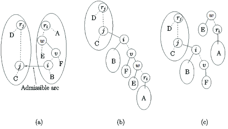
Figure 2: (a) Components before merger (b) Before pushing flow along admissible path from $r_{i}$ to $r_{j}$ (c) New components generated when arc $(w,v)$ leaves the current forest due to insufficient residual capacity.

If no admissible arc is found, $d(w)$ is increased by $1$ unit for all lowest label nodes $w$ in the component. The algorithm terminates when there are no active nodes with label $<n$. At termination all $n$ labeled nodes form the source set of the min-cut.

The active component to be processed in each iteration can be selected arbitrarily. There are two variants of the pseudoflow algorithm: (i) the lowest label pseudoflow algorithm, where an active component with the lowest labeled root is processed at each iteration; and (ii) the highest label algorithm, where an active component with the highest labeled root node is processed at each iteration.

The first stage of HPF terminates with the min-cut and a pseudoflow. The second stage converts this pseudoflow to a maximum feasible flow. This is done by flow decomposition. Hence representing the flow as the sum of flows along a set of $s$-$t$ paths, and flows along a set of directed cycles, such that no two paths or cycles are comprised of the same set of arcs ([20], pages 79-83). This stage can be done in $O(m\log n)$ by flow decomposition in a related network, [12]. Our experiments, like the experiments in [17], indicate that the time spent in flow recovery is small compared to the time to find the min-cut.

  /*
Min-cut stage of HPF algorithm.
*/ procedure HPF ($V_{st},A_{st},c$): begin SimpleInit ($A_{s},A_{t},c$); while $\exists$ an active component $T$ with root $r$, where $d(r)<n$, do $w\leftarrow r$; while $w\neq\emptyset$ do if $\exists$ admissible arc $(w,v)$ do Merger (${\rm root}(w),\cdots,w,v,\cdots,{\rm root}(v)$); $w\leftarrow\emptyset$; else do if $\exists y\in T:({\rm current}(y)=w)\wedge(d(y)=d(w))$ do $w\leftarrow y$; else do {relabel} $d(w)\leftarrow d(w)+1$; $w\leftarrow{\rm current}(w)$; end  

Figure 3: The min-cut stage of the HPF algorithm. At termination all nodes in label-$n$ components are the source set of the min-cut.

II-C Boykov’s and Kolmogorov’s Augmenting Paths Algorithm

Boykov’s and Kolmogorov’s augmenting paths algorithm, BK, [13] attempts to improve on standard augmenting path techniques on graphs in vision. Given that $|C|$ is the capacity of a minimum cut, the theoretical complexity of this algorithm is $O(mn^{2}|C|)$. Similarly to Ford–Fulkerson’s algorithm [15], the BK algorithm’s complexity is only pseudo-polynomial. In this it differs from the other algorithms studied here, all of which have strongly polynomial time complexity. Despite of that, it has been demonstrated in [13] that in practice on a set of vision problems, the algorithm works well.

At heart of the augmenting paths approach is the use of search trees for detecting augmenting paths from $s$ to $t$. Two such trees, one from the source, $T_{S}$, and the other from the sink, $T_{T}$ are constructed, where $T_{S}\cap T_{T}=\emptyset$. The trees are constructed so that in $T_{S}$ all edges from each parent node to its children are non-saturated and in $T_{T}$, edges from children to their parents are non-saturated.

Nodes that are not associated with a tree are called free. Nodes that are not free can be tagged as active or passive. Active nodes have edges to at least one free node, while passive nodes have no edges connecting them to a free node. Consequentially trees can grow only by connecting, through a non-saturated edge, a free node to an active node of the tree. An augmenting path is found when an active node in either of the trees detects a neighboring node that belongs to the other tree.

At the initialization stage the search tree, $T_{S}$ contains only the source node, $s$ and the search tree $T_{T}$ contains only the sink node $t$. All other nodes are free.

Each iteration of the algorithm consists of the following three stages:

Growth In this stage the search trees $T_{S}$ and $T_{T}$ expand. For all active nodes in a tree, $T_{S}$ or $T_{T}$, adjacent free nodes, which are connected through non-saturated edge, are searched. These free nodes become members of the corresponding search tree. The growth stage terminates when the search for an active node from one tree, finds an adjacent (active) node that belongs to the other tree. Thus, an augmenting path from $S$ to $T$ was found.

Augmentation Upon finding the augmenting path, the maximum flow possible is being pushed from $s$ to $t$. This implies that at least one edge will be saturated. Thus, for at least one node in the trees $T_{S}$ and $T_{T}$ the edge connecting it to its parent is no longer valid. The augmentation phase may split the search trees $T_{S}$ and $T_{T}$ into forests. Nodes for which the edges connecting them to their parent become saturated are called orphans.

Adoption In this stage the tree structure of $T_{S}$ and $T_{T}$ is restored. For each orphan, created in the previous stage, the algorithm tries to find a new valid parent. The new parent should belong to the same set, $T_{S}$ or $T_{T}$, as the orphan node and has a non-saturated edge to the orphan node. If no parent is found, then the orphan node and all its children become free and the tree structure rooted in this orphan is discarded. This stage terminates when all orphan nodes are connected to a new parent or are free.

The algorithm terminates when there are no more active nodes and the trees are separated by saturated edges. Thus, the maximum flow is achieved and the corresponding minimum-cut is $S=T_{S}$ and $T=T_{T}$.

It is interesting to note that there are two speed-ups for the BK-algorithm. The first one is an option to reuse search trees from one maxflow computation to the next as described in [21]. This option does not apply in our setting as the instances are not modified. The other speed-up is due to capacity scaling [22]. We would have liked to test this version but we are not aware of any publicly available implementation.

II-D The Partial Augment-Relabel

The Partial Augment-Relabel algorithm, PAR, devised by Goldberg, [14] searches for the shortest augmenting path and it maintains a flow (rather than a pseudoflow or preflow). A relabeling mechanism is utilized by the algorithm to find the augmenting paths.

The algorithm starts at $s$ and searches for admissible, non-saturated, arcs in a depth-first search manner. An arc $(x,y)$ is admissible if the label of its associated nodes is equal, $d(x)=d(y)$. At each iteration, the algorithm maintains a path from $s$ to $v\in V$ and tries to extend it. If $v$ has an admissible arc, $(v,w)$, the path is extended to $w$. If no such admissible arc is found, the algorithm shrinks the path, making the predecessor of $v$ on the path the current node and relabels $v$. At each iteration, the search terminates either if $w=t$, or if the length of the path reaches some predefined value, $k$, or if $v$, the current node has no outgoing admissible arcs. For $k=\Theta(\sqrt{m})$, PAR has a complexity of $O(n^{2}\sqrt{m})$ [14].

In order to achieve better performance in practice, the same gap and global heuristics mentioned in Section II-A, for PRF, can be applied here for the PAR algorithm.

III Experimental Setup

The PRF, HPF and the BK algorithms are compared here by running them on the same problem instances and on the same hardware setup. The run-times of the highest level variant of the PRF algorithm and of PAR are reported in [14] for a subset of the problems used here. Since the source code for the PAR implementation is not made available, the PAR performance is evaluated here through the speedup factor of PAR with respect to the highest level variant of the PRF algorithm for each instance reported in the above paper.

As suggested by Chandran and Hochbaum [17] we use the highest label version for the HPF algorithm. The latest version of the code (version 3.23) is available at [23]. The highest level variant of the PRF algorithm is considered to have the best performance in practice [24]. We use the highest-level PRF implementation Version 3.5, [25]. Note that the latest implementation of the Push-Relabel method is actually denoted by HI_PR, which indicates that the highest-label version is used. We refer to it as PRF, to indicate that it is the same algorithm which was reported in [24]. For the BK algorithm, a library implementation was used [26]. In order to utilize the library for solving problems in DIMACS format, a wrapping code, wrapper, was written. This wrapper reads the DIMACS files and calls the library’s functions for constructing and solving the problem. The part that reads the DIMACS files, under the required changes, is similar to the code used in the HPF implementation. One should note that the compilation’s setup and configuration of the library have great effect on the actual running times of the code. In our tests the shortest running times were achieved using the following compilation line g++ -w -O4 -o <output_file_name> -DNDEBUG -DBENCHMARK graph.cpp maxflow.cpp <wrapper_implementation_file>.

Every problem instance was run $5$ times and we report the average time of the three runs. These are reported for the three different stages of the algorithm (Initialization, Compute Min-Cut and Flow recovery). As detailed in section I, breaking down the run-times provides insight into the algorithms’ performance and allows for better comparison. Since for many computer-vision applications only the min-cut solution is of importance (e.g. [2, 27, 4, 5, 6, 7, 28, 29, 30, 31, 32, 33, 34, 35, 36]), the most relevant evaluation is of the initialization and min-cut times.

III-A Computing Environments

Our experiments were conducted on a machine with x86_64 Dual-Core AMD Opteron(tm) Processor at 2.4 GHz with 1024 KB level 2 cache and 32 GB RAM. The operating system was GNU/Linux kernel release 2.6.18-53.el. The code of all three algorithms, PRF, HPF and BK, was compile with gcc 4.1.2 for the x86_64-redhat-linux platform with $-O4$ optimization flag.

One should note that the relatively large physical memory of the machine allows one to avoid memory swaps between the memory and the swap-file (on the disk) throughout the execution of the algorithms. Swaps are important to avoid since when the machine’s physical memory is small with respect to the problem’s size, the memory swap operation might take place very often. These swapping times, the wait times for the swap to take place, can accumulate to a considerably long run-times. Thus, in these cases, the execution times are biased due to memory constraints, rather than measuring the algorithms’ true computational efficiency. Therefore we chose large physical memory which allows for more accurate and unbiased evaluation of the execution times.

III-B Problem Classes

The test sets used consist of problem instances that arise as min-cut problems in computer vision, graphics, and biomedical image analysis. All instances were made available from the Computer Vision Research Group at the University of Western Ontario [9]. The problem sets used are classified into four types of vision tasks: Stereo vision, Segmentation, Multi-view reconstruction; and Surface fitting. These are detailed in sections III-B1 through III-B3. The number of nodes $n$ and the number of arcs $m$ for each of the problems are given in Table III-B4.

III-B1 Stereo Vision

Stereo problems, as one of the classical vision problems, have been extensively studied. The goal of stereo is to compute the correspondence between pixels of two or more images of the same scene. we use the Venus, Sawtooth [5] and the Tsukuba [28] data-sets. These sequences are made up of piecewise planar objects. Each of the stereo problems, used in this study, consists of an image sequence, where each image in the sequence is a slightly shifted version of its preceding one. A corresponding frame for each sequence is given in Figure 4.

Often the best correspondence between the pixels of the input images is determined by solving a min-cut problem for each pair of images in the set. Thus in order to solve the stereo problem, one has to solve a sequence of min-cut sub-problems all of approximately the same size. Previously reported run-times of these stereo problem [13, 14] disclosed, for each problem, only the summation of the run-times of its min-cut sub-problems. Presenting the summation of the run-times of the sub-problems as the time for solving the entire problem assumes linear asymptotic behaviour of the run-times with respect to the input size. This assumption has not been justified. The run-times here, for the stereo problems, are reported as the average time it takes the algorithm to solve the min-cut sub-problem.

Each of the stereo min-cut sub-problems aims at matching corresponding pixels in two images. The graphs consist of two $4$-neighborhood grids, one for each image. Each node, on every grid, has arcs connecting it to a set of nodes on the other grid. For each of the stereo problems there are two types of instances. In one type, indicated by KZ2 suffix, each node in one image is connected to at most two nodes in the other image. In the second type, indicated by BVZ suffix, each node in one image is connected to up to five nodes in the second image.

$$\begin{array}[]{c c c}\framebox{\includegraphics[width=108.405pt]{sawtooth}}&\framebox{\includegraphics[width=108.405pt]{venus}}&\framebox{\includegraphics[width=127.9171pt]{tsukuba}}\\ Sawtooth&Venus&Tsukuba\\ \end{array}$$

Figure 4: Stereo test sequences (source [9])

III-B2 Multi-view reconstruction

A 3D reconstruction is a fundamental problem in computer vision with a significant number of applications (for recent examples see [37, 6, 7]). Specifically, graph theory based algorithms for this problem were reported in [38, 39, 40].The input for the multi-view reconstruction problem is a set of 2D images of the same scene taken from different perspectives. The reconstruction problem is to construct a 3D image by mapping pixels from the 2D images to voxels complex in the 3D space. The most intuitive example for such a complex would be a rectangular grid, in which the space is divided into cubes. In the examples used here a finer grid, where each voxel is divided into 24 tetrahedral by six planes each passing through a pair of opposite cube edges, is used (See [38] for details). Two sequences are used in this class, Camel and Gargoyle. Each sequence was constructed in three different sizes (referred to as small, middle and large) [41]. Representing frames are presented in Figure 5.

$$\begin{array}[]{c c}\framebox{\includegraphics[width=131.82085pt]{Camel}}&\framebox{\includegraphics[width=97.56714pt]{gargo}}\\ Camel&Gargoyle\\ \end{array}$$

Figure 5: Multi-view test sequences (source [9])

III-B3 Surface fitting

3D reconstruction of an object’s surface from sparse points containing noise, outliers, and gaps is also one of the most interesting problems in computer vision. Under this class we present a single test instance, ”Bunny” (see Fig. 6), constructed in three different sizes. The sequence is part of the Stanford Computer Graphics Laboratory 3D Scanning Repository [10] and consists of $362,272$ scanned points. The goal then to reconstruct the observed object by optimizing a functional that maximizes the number of data points on the 3D grid while imposing some shape priors either on the volume or the surface, such as spatial occupancy or surface area [29]. The ”bunny” corresponding graphs, on which the min-cut problem is solved, are characterized by particularly short paths from $s$ to $t$ [29].

$$\begin{array}[]{c c}\framebox{\includegraphics[width=131.82085pt]{bunnyOrig}}&\framebox{\includegraphics[width=131.82085pt]{bunnyRang}}\\ OriginalImage&ReconstructedSurface\\ \end{array}$$

Figure 6: Bunny Problem Instance - Surface fitting (source [10])

III-B4 Segmentation

Under this group $4$ test sets, referred to as ”Liver”, ”adhead”, ”Babyface” and ”bone” are used. Each set consists of similar instances which differ in the graph size, neighborhood size, length of the path between $s$ and $t$, regional arc consistency (noise), and arc capacity magnitude [42]. For all instances used in this group, the suffices $n$ and $c$ represent the neighborhood type and maximum arc capacities respectively. For example, bone.n6.c10 and babyface.n26.c100, correspond to a $6$ neighborhood and a maximum arc capacity of $10$ units and a $26$ neighborhood with maximum arc capacity of $100$ units respectively. The different bone instances differ in the number of nodes. The grid on the 3 axes x,y and z was made coarser by a factor of 2 on each, thus bone_xy, means that the original problem (bone) was decimated along the x,y axes and it is $1/4$ of its original size; bone_xyz, means that the original problem was decimated along the x,y and z axes and it is $1/8$ of its original size.

Instance			Run-times [Secs]			Slowdown Factor
Name	Nodes	Arcs	PRF	HPF	BK	PRF	HPF	BK
Stereo
sawtoothBVZ	173,602	838,635	1.55	0.76	0.62	2.50	1.23	1
sawtoothKZ2	310,459	2,059,153	4.05	1.87	1.52	2.66	1.23	1
tsukubaBVZ	117,967	547,699	1.09	0.50	0.41	2.66	1.22	1
tsukubaKZ2	213,144	1,430,508	3.42	1.33	1.06	3.23	1.25	1
venusBVZ	174,139	833,168	1.93	0.82	0.66	2.92	1.24	1
venusKZ2	315,972	2,122,772	5.12	2.09	1.66	3.08	1.26	1
Multi-View
camel-lrg	18,900,002	93,749,846	558.65	143.96	225.53	3.88	1	1.57
camel-med	9,676,802	47,933,324	240.30	67.61	83.43	3.55	1	1.23
camel-sml	1,209,602	5,963,582	17.16	6.31	6.46	2.72	1	1.02
gargoyle-lrg	17,203,202	86,175,090	413.26	134.77	432.31	3.07	1	3.21
gargoyle-med	8,847,362	44,398,548	196.26	56.24	226.43	3.49	1	4.03
gargoyle-sml	1,105,922	5,604,568	12.26	5.00	13.86	2.45	1	2.77
Surface Fitting
bunny-lrg	49,544,354	300,838,741	1564.10	305.05	277.02	5.56	1.10	1
bunny-med	6,311,088	38,739,041	129.05	34.47	32.82	3.93	1.05	1
bunny-sml	805,802	5,040,834	10.89	4.12	4.03	2.70	1.02	1
Segmentation
adhead.n26c10	12,582,914	327,484,556	970.74	344.31	407.42	2.82	1	1.18
adhead.n26c100	12,582,914	327,484,556	971.20	362.49	476.04	2.68	1	1.31
adhead.n6c10	12,582,914	75,826,316	219.14	90.17	90.38	2.43	1	1.01
adhead.n6c100	12,582,914	75,826,316	242.43	103.03	123.22	2.35	1	1.20
babyface.n26c10	5,062,502	131,636,370	333.91	245.10	250.15	1.36	1	1.02
babyface.n26c100	5,062,502	131,636,370	378.94	272.26	321.20	1.39	1	1.18
babyface.n6c10	5,062,502	30,386,370	103.27	48.30	35.30	2.93	1.37	1
babyface.n6c100	5,062,502	30,386,370	126.28	58.77	43.89	2.88	1.34	1
bone.n26c10	7,798,786	202,895,861	451.35	160.73	196.26	2.81	1	1.22
bone.n26c100	7,798,786	202,895,861	472.34	168.09	198.73	2.81	1	1.18
bone.n6c10	7,798,786	46,920,181	119.76	41.02	47.79	2.92	1	1.17
bone.n6c100	7,798,786	46,920,181	132.06	43.56	51.88	3.03	1	1.19
bone_subx.n26c10	3,899,394	101,476,818	209.03	79.70	100.23	2.62	1	1.26
bone_subx.n26c100	3,899,394	101,476,818	218.57	81.79	107.43	2.67	1	1.31
bone_subx.n6c10	3,899,394	23,488,978	64.17	20.89	26.57	3.07	1	1.27
bone_subx.n6c100	3,899,394	23,488,978	61.18	22.06	30.29	2.77	1	1.37
bone_subxy.n26c10	1,949,698	50,753,434	99.59	39.51	48.25	2.52	1	1.22
bone_subxy.n26c100	1,949,698	50,753,434	101.13	40.00	51.04	2.53	1	1.28
bone_subxy.n6c10	1,949,698	11,759,514	27.22	10.04	12.09	2.71	1	1.20
bone_subxy.n6c100	1,949,698	11,759,514	27.66	10.56	13.62	2.62	1	1.29
bone_subxyz.n26c10	983,042	25,590,293	48.07	18.89	23.69	2.54	1	1.25
bone_subxyz.n26c100	983,042	25,590,293	48.83	19.39	25.41	2.52	1	1.31
bone_subxyz.n6c10	983,042	5,929,493	11.95	4.85	5.95	2.46	1	1.23
bone_subxyz.n6c100	983,042	5,929,493	12.05	5.14	6.54	2.34	1	1.27
bone_subxyz_subx.n26c10	491,522	12,802,789	22.96	9.36	11.27	2.45	1	1.20
bone_subxyz_subx.n26c100	491,522	12,802,789	23.55	9.52	11.55	2.47	1	1.21
bone_subxyz_subx.n6c10	491,522	2,972,389	5.47	2.37	2.75	2.31	1	1.16
bone_subxyz_subx.n6c100	491,522	2,972,389	5.56	2.47	2.89	2.25	1	1.17
bone_subxyz_subxy.n26c10	245,762	6,405,104	10.99	4.63	5.60	2.37	1	1.21
bone_subxyz_subxy.n26c100	245,762	6,405,104	11.06	4.74	5.79	2.33	1	1.22
bone_subxyz_subxy.n6c10	245,762	1,489,904	2.55	1.14	1.34	2.24	1	1.18
bone_subxyz_subxy.n6c100	245,762	1,489,904	2.59	1.21	1.39	2.14	1	1.15
liver.n26c10	4,161,602	108,370,821	272.63	123.61	112.40	2.43	1.10	1
liver.n26c100	4,161,602	108,370,821	297.88	132.48	128.60	2.32	1.03	1
liver.n6c10	4,161,602	25,138,821	82.11	35.24	32.02	2.56	1.10	1
liver.n6c100	4,161,602	25,138,821	96.38	40.36	43.60	2.39	1	1.08

TABLE I: Vision problems: Graph sizes with combined Initialization and Minimum-cut run-times and their corresponding speedup factors. Each problem’s fastest run-time is set in boldface. The speedup factor states how much an algorithm runs compared to the fastest algorithm

IV Results

IV-A Run-times

In this study, the comparison of the PRF’s, HPF’s and BK’s run-times are indicated for the three stages of the algorithms: (i) initialization, $t_{init}$; (ii) minimum-cut, $t_{minCut}$; and (iii) maximum-flow, $t_{maxFlow}$. As these data is unknown for the PAR algorithm, the comparison of these three algorithms with respect to PAR is addressed differently, by running PRF on our setup and deducing the PAR run-times by multiplying the measured PRF time by the speedup factor reported in [14]. This is explained in Section IV-B.

As already indicated, the most relevant times in this study are the times it takes each of the algorithms to complete the computation of the min-cut, thus $t_{init}+t_{minCut}$. These are graphically presented in Figure 7 and detailed in Table III-B4. The Slowdown Factor, reported in table III-B4 for each algorithm, for every problem instance, is the ratio of the time it takes the algorithm to complete the computation of the minimum-cut divided by the minimum time it took any of the algorithms to complete this computation.

Figure 77(a) presents the run-times for the stereo vision problem sets. The input’s size, for these problems is small, with respect the the other problem sets. For these small problem instances, the BK algorithm is doing better than PRF (with average Slowdown factor of $2.86$, which corresponds to average difference in the running time of $2.0$ Seconds) and slightly better than HPF (slowdown factor of $1.24$, which corresponds to a running time difference of $0.24$ Seconds). For the Multi-view instances HPF presents better results than both algorithms with average slowdown factors of $1.46$ with respect to BK and $3.19$ with respect to PRF. These correspond to differences in the running times of $95$ and $170$ seconds respectively. This is illustrated in Figure 77(b). Figure 7(c) shows that the BK algorithm is more suitable for solving the surface fitting instances. This is attributed to the fact that these problems are characterized by particularly short s-t paths. In these instances, the slowdown factors of HPR and PRF are $1.05$ (correspond to an average difference of $9$ seconds) and $4.06$ (difference of $454$ seconds). The running times for the Segmentation problems class are depicted in Figure 77(d). There are $36$ segmentation problems. In a subset of $5$ segmentation problems BK achieved shorter running times. In this subset the BK’s average slowdown factors are $1.19$ ($9.24$ seconds difference) and $2.62$ ($106$ seconds difference in the running time) with respect to HPF and PRF respectively. On the rest of the $31$ segmentation problems, HPF shows shorter running times with slowdown factors of $1.18$ ($14.22$ seconds difference) with respect to BK and $2.62$ ($101.39$ seconds difference) with respect to PRF.

A total of $51$ problem instances were tested within the scope of this study. The HPF algorithm was shown to be better in $37$ problem instances. The BK algorithm achieved better results over the other $14$ problems. The average run-times and slowdown factors of these two subsets are given in Table II.

TABLE II: Average running times and slowdown factors

	PRF	HPF	BK
HPF is better ($37$ problem instances)
Ave. run-time	184.87	72.25	99.69
Ave. slowdown	2.6	1	1.39
BK is better ($14$ problem instances)
Ave. run-time	185.96	53.53	48.00
Ave. slowdown	3.03	1.18	1

(a) Stereo

(b) Multi-View

(c) Surface Fitting

(d) Segmentation

Figure 7: Initialization and Minimum-cut run-times in seconds: 7(a) Stereo Problems; 7(b) Multi-view Problems; 7(c) Surface Fitting; 7(d) Segmentation

In order to allow for the comparison of the times it takes each of the algorithms to complete the computation of only the min-cut phase, the initialization run-times are presented in Figure 8 and detailed in Appendix A, Tables III-B4 – III-B4. Ideally one should be able to evaluate the minimum-cut processing times by subtracting the initialization times in Tables III-B4 – III-B4 from the corresponding times in Table III-B4. However, as described in Section I, while the BK and HPF algorithms only read the problem’s data and allocate memory, the PRF algorithm has some additional logic in its initialization phase. Consequentially, one can not evaluate PRF’s min-cut processing times by this substraction. To accomplish that, one has to account for the time it takes the PRF algorithm to compute the additional logic implemented with the initialization stage. Figure 8 shows that for all problem instances, the PRF’s initialization times ($t_{init}$) are $2-3$ times longer than BK’s and HPF’s times. While these times were excluded from the total execution times reported in [13] and [14], Figure 8 strongly suggests that these initialization times are significant with respect to to the min-cut computation times ($t_{minCut}$) and should not be disregarded.

(a) Stereo

(b) Multi-View

(c) Surface Fitting

(d) Segmentation

Figure 8: Initialization run-times in seconds: 8(a) Stereo Problems; 8(b) Multi-view Problems; 8(c) Surface Fitting; 8(d) Segmentation

The actual maximum-flow plays a less significant role in solving computer vision problems. Yet, for the sake of completeness, the maximum flow computation times of the algorithms $(t_{init}+t_{minCut}+t_{maxFlow})$ are reported in Figure 9 and in Tables III-B4 – III-B4.

(a) Stereo

(b) Multi-View

(c) Surface Fitting

(d) Segmentation

Figure 9: Initialization, Minimum cut and Maximum Flow run-times in seconds: 9(a) Stereo Problems; 9(b) Multi-view Problems; 9(c) Surface Fitting; 9(d) Segmentation

IV-B Comparison to Partial Augment-Relabel

The PAR run-times, on our hardware setup, are deduced from the speedup factor for PAR with respect to the highest level variant of the PRF which are reported in [14]. The paper above reports only the summation of the min-cut and max-flow run-times (without initialization), $t_{minCut}+t_{maxFlow}$ . Therefore, to enable a fair comparison we use the min-cut and max-flow run-times of the other algorithms as well. For $t_{PAR}^{G}$ and $t_{PRF}^{G}$, the run-times reported in [14] for the PAR and PRF algorithms respectively, the estimated run-time of PAR, $\hat{t}_{PAR}$, on our hardware is:

$$\hat{t}_{PAR}=\frac{t_{PAR}^{G}}{t_{PRF}^{G}}~{}(t_{minCut}^{PRF}+t_{maxFlow}^{PRF})$$

where $t_{minCut}^{PRF}$ and $t_{maxFlow}^{PRF}$ are the corresponding run-times of the PRF algorithm measured on the hardware used in this study.

The comparison results are given in Figure 10 for all problem instances reported in [14]. As reported in [14], the PAR algorithm indeed improves on PRF. HPF outperforms PAR for all problem instances. It is noted that in this comparison of the run-times that exclude initialization PAR’s performance is still inferior to that of HPF. If one were to add the initialization time then the relative performance of PAR as compare to HPF would be much worse since the initialization used has time consuming logic in it as note previously in Section I and is shown in Figure 8. In terms of comparing PAR to BK, Figure 10 shows that PAR is inferior to BK for small problem instances, but performs better for larger instances.

(a) Stereo

(b) Multi-View

(c) Segmentation

Figure 10: PAR, PRF, HPF, BK Minimum cut run-times in seconds: 10(a) Stereo Problems; 10(b) Multi-view Problems; 10(c) Segmentation

IV-C Memory Utilization

Measuring the actual memory utilization is of growing importance, as advances in acquisition systems and sensors allow higher image resolution, thus larger problem sizes.

The memory utilization of each of the algorithms is a result of two factors: (i) the data each algorithm maintains in order to solve the problem. For example, the BK algorithm must maintain a flow $f$, the list of active nodes and a list of all orphans (see Section II-C); and (ii) the efficiency of the specific implementation’s memory allocation in each implementation. The first factor can be analytically assessed by carefully examining the algorithm. The latter, however, must be evaluated empirically. It is important to note that both do not necessarily grow linearily with the problem size. The memory usage was read directly out of the /proc/[process]/statm file for each implementation and for each problem instance. One should note that the granularity of the information in this file is the page-file size, thus $4096$ Bytes.

Figure 11 summarizes the results of the memory utilization for BK (solid blue line), HPF (dashed green line) and PRF (dotted red line) algorithms. These are detailed in Appendix B, Table III-B4. The X-axis in Figure 11 is the input size. A Problem’s input size is the number of nodes, $n$ plus the number of arcs, $m$, in the problem’s corresponding graph: $input~{}size=n+m$. The number of nodes, $n$, and the number of arcs, $m$, for each of the problems are given in Table III-B4. The Y-axis is the memory utilization in Mega- Bytes.

Both BK and PRF algorithms use on average 10% more memory than the HPF algorithm. For problem instances with large number of arcs, the PRF and BK require 25% more memory. This becomes critical when the problem size is considerably large, with respect to the machine’s physical memory. In these cases the execution of the algorithms requires a significant amount of swapping memory pages between the physical memory and the disk, resulting in longer execution times.

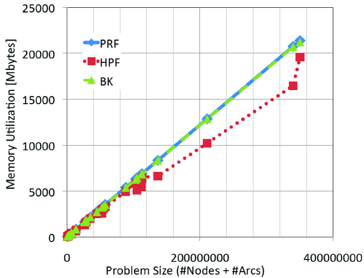
Figure 11: Memory Utilization Vs. Input size

IV-D Summary

Figure 12 is a graphical summary of the run-times of each of the algorithms for the min-cut task ($t_{init}+t_{minCut}$) depending on the problem size. Figure 12 and tables III-B4 and II suggest that the BK and the HPF algorithms generate comparable results. The the first, BK, is more suited for small problem instances (less then $1,000,000$ graph elements (#Nodes + #Arcs)) or for instances that are characterized by a short paths from $s$ to $t$. The latter, HPF, might be used for all other general larger problems. Figure 10 shows that this also holds for PRF’s revised version, the partial augment-relabel (PAR) algorithms, for all vision problem instances examined in this study. In detail, out of the $51$ instances BK is dominating $14$ times with an average running time of $48$ seconds on these instances. HPF on the other hand has an averaged running time of $54$ seconds and therefor the HPF algorithm has a slowdown factor of $1.18$ with respect to BK. On the remaining 37 instances HPF is dominating with an average running time of $72$ seconds. It takes BK $100$ seconds in average to finish on theses instances, whitch results in a slowdown factor of $1.39$ for BK with respect to HPF.

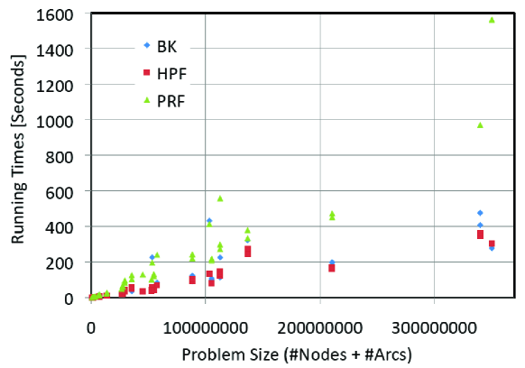
Figure 12: Minium-cut Execution times (Initialization and minimum-cut phases) with respect to the problems’ size

V Conclusions

This paper presents the results of a comprehensive computational study on vision problems, in terms of execution times and memory utilization, of four algorithms, which optimally solve the s-t minimum cut and maximum flow problems: (i) Goldberg’s and Tarjan’s Push-Relabel; (ii) Hochbaum’s pseudoflow; (iii) Boykov’s and Kolmogorov’s augmenting paths; and (iv) Goldberg’s partial augment-relabel.

The results show that the BK algorithm is more suited for small problem instances (less then $1,000,000$ graph elements, thus vertices and arcs) or for instances that are characterized by short paths from $s$ to $t$, the HPF algorithm is better suited for all other general larger problems. In terms of memory utilization, the HPF algorithm has better memory utilization with up to 25% saved in memory allocation as compared to BK and PRF.

Our results are of significance because it has been widely accepted that both BK and PRF algorithms were the fastest algorithms in practice for the min-cut problem. This was shown not to hold in general [17], and here for computer vision in particular. This, with the availability of HPF algorithm’s source-code (see [23]), makes HPF the perfect tool for the growing number of computer vision applications which incorporate the min-cut problem as a sub-routine.

The current strategy of speeding up computers is to increment the number of processors instead of increasing the computing power of a single one. This development suggests that a parallelization of the algorithm would be beneficial. We expect the HPF algorithm to behave well with respect to parallel implementations as well.

Appendix A Run-times

TABLE III: Initialization stage run-times: Stereo Vision problems

TABLE IV: Initialization stage run-times: Multi-View problems

TABLE V: Initialization stage run-times: Surface Fitting problems

TABLE VI: Initialization stage run-times: Segmentation problems

TABLE VII: Total run-times of the Initialization and Min-cut and Max-flow stages - Stereo Vision problems

TABLE VIII: Total run-times of the Initialization and Min-cut and Max-flow stages - Multi-View problems

TABLE IX: Total run-times of the Initialization and Min-cut and Max-flow stages - Surface Fitting problems

TABLE X: Total run-times of the Initialization and Min-cut and Max-flow stages - Segmentation problems

Appendix B Memory Utilization

TABLE XI: Memory Utilization in [MBytes]

References

- [1] R. Ahuja, T. Magnanti, and J. Orlin, Network Flows: Theory, Algorithms, and Applications. Prentice-Hall, 1993.
- [2] D. Hochbaum, “An efficient algorithm for image segmentation, markov random fields and related problems,” J. ACM, vol. 48, no. 4, pp. 686–701, 2001.
- [3] D. S. Hochbaum, “Polynomial time algorithms for ratio regions and a variant of normalized cut,” Pattern Recognition and Machine Intelligence IEEE Transactions on, vol. 32, no. 5, pp. 889–898, 2009.
- [4] D. Hochbaum and V. Singh, “An efficient algorithm for co-segmentation,” in International Conference on Computer Vision (ICCV), 2009.
- [5] D. Scharstein, R. Szeliski, and R. Zabih, “A taxonomy and evaluation of dense two-frame stereo correspondence algorithms,” in Proc. IEEE Workshop on Stereo and Multi-Baseline Vision (SMBV 2001), Dec. 9–10, 2001, pp. 131–140.
- [6] S. N. Sinha, D. Steedly, R. Szeliski, M. Agrawala, and M. Pollefeys, “Interactive 3d architectural modeling from unordered photo collections,” in SIGGRAPH Asia ’08: ACM SIGGRAPH Asia 2008 papers. New York, NY, USA: ACM, 2008, pp. 1–10.
- [7] N. Snavely, S. M. Seitz, and R. Szeliski, “Photo tourism: Exploring photo collections in 3d,” ACM Transactions on Graphics, vol. 25(3), August 2006.
- [8] J. Starck and A. Hilton, “Surface capture for performance-based animation,” IEEE Computer Graphics and Applications, vol. 27, no. 3, pp. 21–31, 2007.
- [9] Computer Vision Research Group, “Max-flow problem instances in vision,” University of Western Ontario, Tech. Rep., accessed Oct 2009, http://vision.csd.uwo.ca.
- [10] Stanford Computer Graphics Laboratory, “”the stanford 3d scanning repository”,” Stanford, Palo-Alto, CA, USA, Tech. Rep., accessed Oct 2009, http://graphics.stanford.edu/data/3Dscanrep/.
- [11] A. V. Goldberg and R. E. Tarjan, “A new approach to the maximum-flow problem,” J. ACM, vol. 35, no. 4, pp. 921–940, 1988.
- [12] D. S. Hochbaum, “The pseudoflow algorithm: A new algorithm for the maximum-flow problem,” Operations Research, vol. 56, no. 4, pp. 992–1009, 2008. [Online]. Available: http://or.journal.informs.org/cgi/content/abstract/56/4/992
- [13] Y. Boykov and V. Kolmogorov, “An experimental comparison of min-cut/max-flow algorithms for energy minimization in vision,” IEEE Transactions on Pattern Analysis and Machine Intelligence, vol. 26, no. 9, pp. 1124–1137, 2004.
- [14] A. Goldberg, “The partial augment–relabel algorithm for the maximum flow problem,” Algorithms - ESA 2008, pp. 466–477, 2008.
- [15] L. Ford and D. Fulkerson, “Maximal flow through a network,” Canadian Journal of Math., vol. 8, no. 3, pp. 339–404, 1956.
- [16] D. D. Sleator and R. E. Tarjan, “A data structure for dynamic trees,” in STOC ’81: Proceedings of the thirteenth annual ACM symposium on Theory of computing. New York, NY, USA: ACM, 1981, pp. 114–122.
- [17] B. Chandran and D. Hochbaum, “A computational study of the pseudoflow and push-relabel algorithms for the maximum flow problem,” Operations Research, vol. 57, no. 2, pp. 358 – 376, 2009.
- [18] H. Lerchs and I. Grossman, “Optimum design of open pit mines,” Transactions, C.I.M, vol. 68, pp. 17–24, 1965.
- [19] D. S. Hochbaum and J. B. Orlin, “Simplifications and speedups of the pseudoflow algorithm,” UC Berkeley manuscript, 2009.
- [20] R. K. Ahuja, M. Kodialam, A. K. Mishra, and J. B. Orlin, “Computational investigations of maximum flow algorithms,” European Journal of Operational Research, vol. 97, no. 3, pp. 509 – 542, 1997. [Online]. Available: http://www.sciencedirect.com/science/article/B6VCT-3SWXMSD-8/2/8d88b6f35cdd701679f1f5b9a328cdbc
- [21] P. Kohli and P. H. S. Torr, “Effciently solving dynamic markov random fields using graph cuts,” in ICCV ’05: Proceedings of the Tenth IEEE International Conference on Computer Vision. Washington, DC, USA: IEEE Computer Society, 2005, pp. 922–929.
- [22] O. Juan and Y. Boykov, “Capacity scaling for graph cuts in vision,” in ICCV, 2007, pp. 1–8.
- [23] D. S. Hochbaum, “HPF Implementation Ver. 3.3,” http://riot.ieor.berkeley.edu/riot/Applications/Pseudoflow/maxflow.html (accessed January 2010).
- [24] B. V. Cherkassky and A. V. Goldberg, “On implementing the push—relabel method for the maximum flow problem,” Algorithmica, vol. 19, no. 4, pp. 390–410, 12 1997.
- [25] A. V. Goldberg, “Hi-level variant of the push-relabel (ver. 3.5),” http://www.avglab.com/andrew/soft.html (accessed January 2010).
- [26] V. Kolmogorov, “An implementation of the maxflow algorithm,” http://www.cs.ucl.ac.uk/staff / V.Kolmogorov / software.html (accessed January 2010).
- [27] D. S. Hochbaum, “Efficient and effective image segmentation interactive tool,” in BIOSIGNALS 2009 - International Conference on Bio-inspired Systems and Signal Processing, 2009, pp. 459–461.
- [28] Y. Nakamura, T. Matsuura, K. Satoh, and Y. Ohta, “Occlusion detectable stereo – occlusion patterns in camera matrix,” Computer Vision and Pattern Recognition, IEEE Computer Society Conference on, vol. 0, p. 371, 1996.
- [29] V. Lempitsky and Y. Boykov, “Global optimization for shape fitting,” in Proc. IEEE Conference on Computer Vision and Pattern Recognition CVPR ’07, Jun. 17–22, 2007, pp. 1–8.
- [30] S. Ali and M. Shah, “Human action recognition in videos using kinematic features and multiple instance learning,” IEEE Trans, Pattern Analysis and Machine Intelligence, vol. 32, no. 2, pp. 288–303, 2010.
- [31] Y. Boykov and D. Huttenlocher, “A new bayesian framework for object recognition,” Computer Vision and Pattern Recognition, IEEE Computer Society Conference on, vol. 2, p. 2517, 1999.
- [32] I. Cox, S. Rao, and Y. Zhong, ““ratio regions”: a technique for image segmentation,” vol. 2, Aug 1996, pp. 557–564 vol.2.
- [33] V. Kwatra, I. Essa, A. Bobick, and N. Kwatra, “Texture optimization for example-based synthesis,” in SIGGRAPH ’05: ACM SIGGRAPH 2005 Papers. New York, NY, USA: ACM, 2005, pp. 795–802.
- [34] S. Roy and I. J. Cox, “A maximum-flow formulation of the n-camera stereo correspondence problem,” in Proc. Sixth International Conference on Computer Vision, Jan. 4–7, 1998, pp. 492–499.
- [35] J. Shi and J. Malik, “Normalized cuts and image segmentation,” Ieee Transactions On Pattern Analysis and Machine Intelligence, vol. 22, no. 8, pp. 888–905, AUG 2000.
- [36] B. Thirion, B. Bascle, V. Ramesh, and N. Navab, “Fusion of color, shading and boundary information for factory pipe segmentation,” Computer Vision and Pattern Recognition, IEEE Computer Society Conference on, vol. 2, p. 2349, 2000.
- [37] I. Ideses, L. Yaroslavsky, and B. Fishbain, “Real-time 2d to 3d video conversion,” Journal of Real-Time Image Processing, vol. 2, no. 1, pp. 3–9, 2007.
- [38] V. Lempitsky, Y. Boykov, and D. Ivanov, “Oriented visibility for multiview reconstruction,” in Computer Vision ECCV 2006, ser. Lecture Notes in Computer Science, A. Leonardis, H. Bischof, and A. Pinz, Eds. Springer Berlin / Heidelberg, 2006, vol. 3953, pp. 226–238. [Online]. Available: http://dx.doi.org/10.1007/11744078_18
- [39] D. Snow, P. Viola, and R. Zabih, “Exact voxel occupancy with graph cuts,” in Proc. IEEE Conference on Computer Vision and Pattern Recognition, vol. 1, Jun. 13–15, 2000, pp. 345–352.
- [40] G. Vogiatzis, P. Torr, and R. Cipolla, “Multi-view stereo via volumetric graph-cuts,” in Computer Vision and Pattern Recognition (CVPR), vol. 2, 2005, pp. 391 – 398.
- [41] V. L. Yuri Boykov, “From photohulls to photoflux optimization,” in British Machine Vision Conference (BMVC), vol. III, Sept 2006, pp. 1149–1158.
- [42] Y. Boykov and G. Funka-Lea, “Graph cuts and efficient n-d image segmentation,” International Journal of Computer Vision, vol. 70, no. 2, p. 109131, 2006. [Online]. Available: http://dx.doi.org/10.1007/s11263-006-7934-5