Retired A Stars and Their Companions VI.
A Pair of Interacting Exoplanet Pairs Around the Subgiants 24 Sextanis and HD 200964¹

Abstract

We report radial velocity measurements of the G-type subgiants 24 Sextanis (=HD 90043) and HD 200964. Both are massive, evolved stars that exhibit periodic variations due to the presence of a pair of Jovian planets. Photometric monitoring with the T12 0.80 m APT at Fairborn Observatory demonstrates both stars to be constant in brightness to $\leq 0.002$ mag, thus strengthening the planetary interpretation of the radial velocity variations. 24 Sex b, c have orbital periods of 452.8 days and 883.0 days, corresponding to semimajor axes 1.333 AU and 2.08 AU, and minimum masses 1.99 $M_{\rm Jup}$ and 0.86 $M_{\rm Jup}$, assuming a stellar mass $M_{\star}=$ 1.54 $M_{\odot}$. HD 200964 b, c have orbital periods of 613.8 days and 825.0 days, corresponding to semimajor axes 1.601 AU and 1.95 AU, and minimum masses 1.99 $M_{\rm Jup}$ and 0.90 $M_{\rm Jup}$, assuming $M_{\star}=$ 1.44 $M_{\odot}$. We also carry out dynamical simulations to properly account for gravitational interactions between the planets. Most, if not all, of the dynamically stable solutions include crossing orbits, suggesting that each system is locked in a mean motion resonance that prevents close encounters and provides long-term stability. The planets in the 24 Sex system likely have a period ratio near 2:1, while the HD 200964 system is even more tightly packed with a period ratio close to 4:3. However, we caution that further radial velocity observations and more detailed dynamical modelling will be required to provide definitive and unique orbital solutions for both cases, and to determine whether the two systems are truly resonant.

1. Introduction

The giant planets thus far discovered around other stars exhibit a wide variety of orbital characteristics that are very different from the properties of the planets in our Solar System. For example, exoplanets rarely reside in circular orbits and many of them have semimajor axes 1 to 2 orders of magnitude smaller than those of Jupiter and Saturn. However, at least one characteristic of exoplanets appears to be shared with the constituents of the Solar System: planets often come in bunches. As Wright et al. 2009 recently showed, 28% of apparently singleton exoplanets are later discovered to reside in systems containing two or more components. As the precision and time baselines of Doppler surveys increase, and as more planets are discovered from wide-field transit surveys (bakos09b; wasp1), direct imaging (marois08; kalas08), and microlensing (gaudi08; gould10), the currently measured multiplicity rate will likely prove to be a lower bound.

Multiplanet systems are manifested in radial velocity (RV) time series as either a single-planet Keplerian motion superimposed atop a partial longer-period orbit, or as multiple, time-resolved orbits (e.g. wright09). Those in the former category will gradually come into focus as the time baselines of Doppler surveys lengthen, and these “trend” systems are becoming recognized as promising direct-imaging targets. The latter category, with their well-characterized orbits, are extremely valuable for understanding the origins of planets and the evolution of their orbital architectures (ford06r).

Observed deviations from pure Keplerian motions reveal gravitational interactions among planets that serve as fossil records of past close encounters and/or convergent orbital migration (malhotra02; wu02). A prime example is the system of planets orbiting $\upsilon$ Andromedae (butler99). ford05b demonstrated through dynamical modeling that the current orbital configuration shows evidence of a violent planet-planet scattering event in the distant past. Similarly, the two Jovian planets in the Gl 876 system currently reside in a mean-motion resonance (MMR) that may be a reflection of differential migration after the planets’ formation (marcy01; lee04; laughlin05). Thus, the discovery of exoplanets in MMRs is strong support for the inward orbital migration that is often invoked to explain the common existence of giant planets well within the canonical “snow line.”

Additionally, gravitational interactions among resonant planets can also place constraints on both the system inclination with respect to the sky, as well as mutual inclinations between the planets, and thereby remove the $\sin{i}$ ambiguity and provide absolute measurements of the planet masses (rivera05; correia10). Interactions observed in certain types of multiplanet systems can reveal the interior structures of gas giant planets in vivid detail. In the dramatic case of the system of planets around HAT-P-13, the inner planet transits its host star and experiences additional gravitational perturbations from an outer planet near 1 AU (bakos09; winn10). Depending on the inclinations of the planets in the system, precise follow-up measurements may provide estimates of the tidal Love number and Q value of the inner planet to a higher precision than is possible for Jupiter (batygin09; mardling10).

We are conducting a Doppler survey of intermediate-mass subgiant stars at the Lick and Keck Observatories with the goal of understanding the influence stellar mass on the physical properties, orbital architectures and multiplicity rates of planetary systems. Our survey has resulted in the discovery of 14 new singleton exoplanets (johnson06; johnson07; johnson08a; peek09; bowler10; johnson10b). In this contribution we announce the discovery of two pairs of Jovian planets orbiting the subgiants 24 Sextanis ($=$HD 90043) and HD 200964.

2. Spectroscopic Observations

We began observations of 24 Sex and HD 200964 at Lick Observatory in 2004–2005 as part of our Doppler survey of intermediate-mass subgiants. Details of the survey, including target selection and observing strategy are given in johnson06b, peek09 and bowler10. In 2007 we expanded our survey of subgiants at Keck Observatory (johnson10b) and we added 24 Sex and HD 200964 to our Keck target list for additional monitoring.

At Lick Observatory, the Shane 3 m and 0.6 m Coude Auxiliary Telescopes (CAT) feed the Hamilton spectrometer (vogt87), and observations at Keck Observatory were obtained using the HIRES spectrometer (vogt94). Doppler shifts are measured from each observation using the iodine cell method described by butler96 (see also marcy92b). A temperature–controlled Pyrex cell containing gaseous iodine is placed at the entrance slit of the spectrometer. The dense set of narrow molecular lines imprinted on each stellar spectrum from 5000 to 6000 Å provides a robust wavelength scale for each observation, as well as information about the shape of the spectrometer’s instrumental response (valenti95).

At Lick, typical exposure times of 60 minutes on the CAT and 5 minutes on the 3 m yield a signal-to-noise ratio (SNR) of $\approx$120 at the center of the iodine region ($\lambda=5500$ Å), providing a velocity precision of 4.0–5.0 m s^-1. At Keck, typical spectra have SNR $\approx 180$ at 5500 Å, resulting in a velocity precision of 1.5–2.0 m s^-1.

In addition to the internal, photon-limited uncertainties, the RV measurements include an additional noise term due to stellar “jitter”—velocity noise in excess of internal errors due to astrophysical sources such as pulsation and rotational modulation of surface features (saar98; wright05). We therefore adopt a jitter value of 5 m s^-1 for our subgiants based on the estimate of johnson10b. This jitter term is added in quadrature to the internal errors before determining the Keplerian orbital solutions. For the dynamical analysis in § 6 we allow the jitter to vary as a free parameter in the fitting process.

3. Stellar Properties

Table 1Stellar Parameters

Parameter	24 Sex	HD 200964
V	6.61 (0.04)	6.64 (0.04)
$M_{V}$	2.17 (0.06)	2.35 (0.07)
B-V	0.92 (0.01)	0.880 (0.009)
Distance (pc)	74.8 (4.9)	68.4 (4.8)
${\rm[Fe/H]}$	-0.03 (0.04)	-0.15 (0.04)
$T_{eff}$ (K)	5098 (44)	5164 (44)
$V_{\rm rot}\sin{i}$ (km s-1)	2.77 (0.5)	2.28 (0.5)
$\log{g}$	3.5 (0.1)	3.6 (0.1)
$M_{*}$ ($M_{\odot}$)	1.54 (0.08)	1.44 (0.09)
$R_{*}$ ($R_{\odot}$)	4.9 (0.08)	4.3 (0.09)
$L_{*}$ ($L_{\odot}$)	14.6 (0.1)	11.6 (0.4)
Age (Gyr)	2.7 (0.4)	3.0 (0.6)
$\log R^{\prime}_{HK}$	-5.1	-5.1

Atmospheric parameters of the target stars are estimated from iodine-free, “template” spectra using the LTE spectroscopic analysis package Spectroscopy Made Easy (SME; valenti96), as described by valenti05 and fischer05b. To constrain the low surface gravities of the evolved stars we used the iterative scheme of valenti09, which ties the SME-derived value of $\log{g}$ to the gravity inferred from the Yonsei-Yale (Y²; y2) stellar model grids. The analysis yields a best-fitting estimate of $T_{\rm eff}$, $\log{g}$, [Fe/H], and $V_{\rm rot}\sin{i}$. The properties of our targets from Lick and Keck are listed in the fourth edition of the Spectroscopic Properties of Cool Stars Catalog (SPOCS IV.; Johnson et al. 2010, in prep). We adopt the SME parameter uncertainties described in the error analysis of valenti05.

The luminosity of each star is estimated from the apparent V-band magnitude and the parallax from Hipparcos (hipp2), together with the bolometric correction from vandenberg03. From $T_{\rm eff}$ and luminosity, we determine the stellar mass, radius, and an age estimate by associating those observed properties with a model from the Y² stellar interior calculations (y2). We also measure the chromospheric emission in the CaII H&K line cores (wright04b), providing an $S$ value on the Mt. Wilson system, which we convert to $R^{\prime}_{HK}$ as per Noyes84. The stellar properties of the host stars are summarized in Table 1.

4. Keplerian Orbital Solutions

In this section we present the RV time series for both stars and the initial orbital analysis, which consists of the sum of two Keplerians without gravitational interaction. In § 6 we present the results of our Newtonian dynamical analysis for each system, which properly accounts for non-Keplerian motion due to gravitational interactions between the planets and host star.

Table 2Orbital Parameters from Non-interacting Two-planet Solution

Parameter	24 Sex b	24 Sex c	HD 200964 b	HD 200964 b
Period (d)	455.2 (3.2)	910 (21)	630.6 (9.3)	829 (21)
Tp (JD)	2454758 (30)	2454941 (30)	2454916 (30)	2455029 (130)
Eccentricity	0.184 (0.029)	0.412 (0.064)	0.111 (0.030)	0.113 (0.076)
K (m s-1)	33.2 (1.6)	23.5 (2.9)	35.2 (2.7)	22.1 (2.3)
$\omega$ (deg)	227 (20)	172.0 (9)	223 (20)	301 (50)
$M_{P}\sin{i}$ ($M_{\rm Jup}$)	1.6 (0.2)	1.4 (0.2)	1.9 (0.2)	1.3 (0.2)
$a$ (AU)	1.41 (0.03)	2.22 (0.06)	1.71 (0.04)	2.03 (0.06)
Lick rms (m s-1)	7.7	…	7.6	…
Keck rms (m s-1)	4.8	…	5.3	…
Jitter (m s-1)	5.0	…	5.0	…
$\sqrt{\chi^{2}_{\nu}}$	1.14	…	1.15	…
Nobs Lick	50	…	61	…
Nobs Keck	24	…	35	…

To search for the best-fitting, two-planet orbital solution for each time series we use the partially-linearized technique presented by wrighthoward, as implemented in the IDL software suite RVLIN. We estimate the parameter uncertainties using a Markov-Chain Monte Carlo (MCMC) algorithm, as described by bowler10.

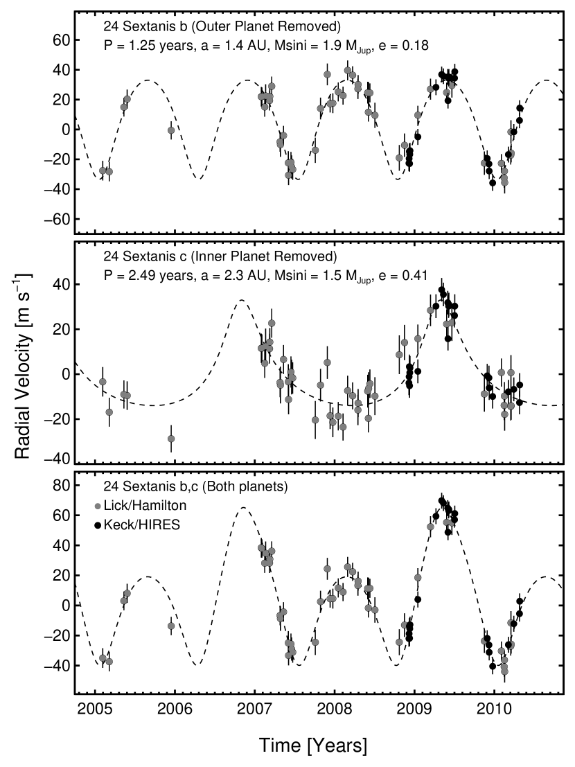
Figure 1.— RV time series and two-Keplerian orbital solution for 24 Sex. Top: Inner planet with the signal from the outer planet removed. The dashed line shows the best-fitting orbital solution for 24 Sex b. Middle: The outer planet with the inner planet removed. The dashed line shows the best-fitting orbital solution for 24 Sex c. Bottom: The full RV time series, with the two-planet solution shown as a dashed line.

4.1. 24 Sextanis

We obtained initial-epoch observations of 24 Sex at Lick Observatory in 2005 February, and since then we have obtained 50 RV measurements. After noticing time-correlated RV variations, we began additional monitoring at Keck Observatory in 2008 December, where we have obtained 24 additional RV measurements. The RVs from both observatories are listed in Table 4, along with the Julian Dates (JD) of observation and the internal measurement uncertainties (without jitter). Fig. 1 shows the RV time series from both observatories, where the error bars represent the quadrature sum of the internal errors and 5 m s^-1 of jitter.

bowler10 reported evidence of a two-planet system around 24 Sex, but the data at the time could not provide a unique orbital solution. An additional season of observations has provided stronger constraints on the possible orbits of the two planets. We fitted a model consisting of two non-interacting planets and a 1.54 $M_{\odot}$ star orbiting their mutual center of mass. We find that two Keplerians provide an acceptable fit to the data with an rms scatter of 6.8 m s^-1 and a reduced $\sqrt{\chi^{2}_{\nu}}$ $=1.14$. The inner planet has a period of $P=455.2\pm 3.2$ days, velocity semiamplitude $K=33.2\pm 1.6$ m s^-1, and eccentricity $e=0.184\pm 0.029$. The outer planet has $P=910\pm 21$ days, $K=23.5\pm 2.9$ m s^-1, and $e=0.412\pm 0.064$. Together with our stellar mass estimate these spectroscopic orbital parameters yield semimajor axes $\{a_{b},a_{c}\}=\{1.41,2.22\}$ AU and minimum planet masses $\{M_{b},M_{c}\}\sin{i}=\{1.6,1.4\}$ $M_{\rm Jup}$. A more detailed, dynamical analysis presented in § 6 revises this two-Keplerian solution under the constraint of long-term stability.

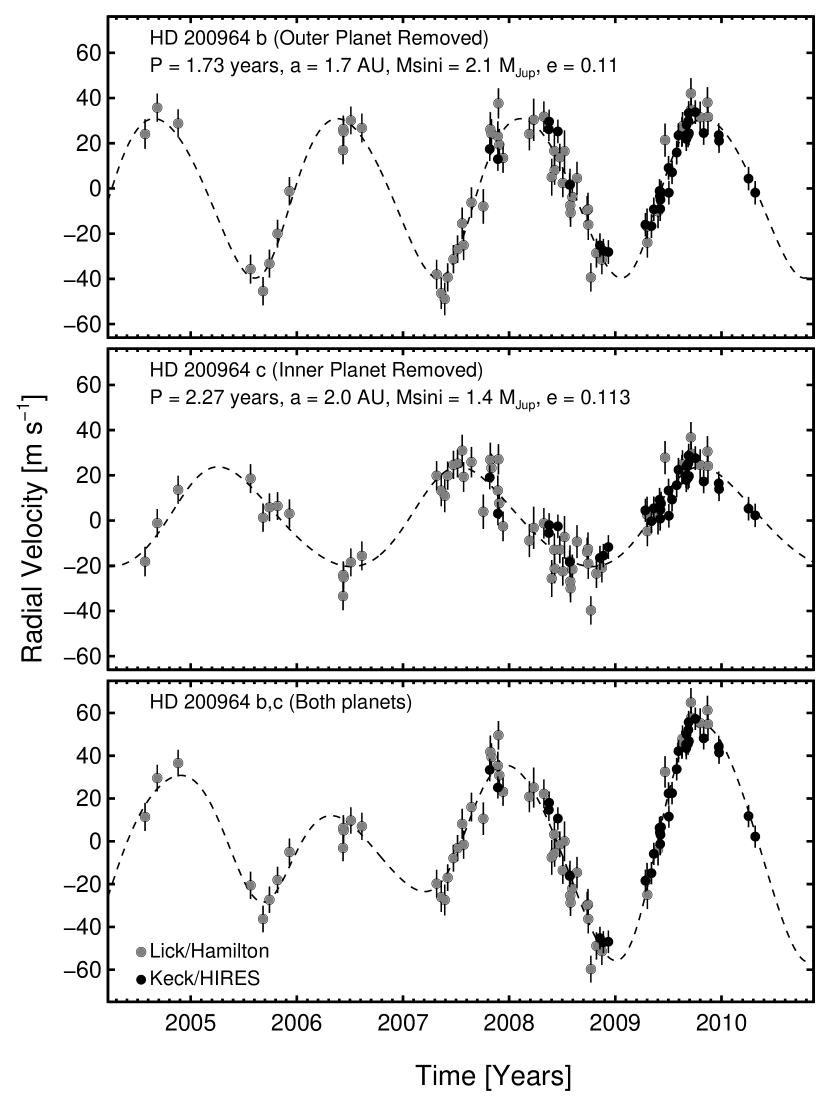
Figure 2.— RV time series and two-Keplerian orbital solution for HD 200964. Top: Inner planet with the signal from the outer planet removed. The dashed line shows the best-fitting orbital solution for HD 200964 b. Middle: The outer planet with the inner planet removed. The dashed line shows the best-fitting orbital solution for HD 200964 c. Bottom: The full RV time series, with the two-planet solution shown as a dashed line.

4.2. HD 200964

We began monitoring HD 200964 at Lick Observatory in 2007 July and have obtained 61 RV measurements. Time-correlated variations in the star’s RVs prompted additional monitoring at Keck Observatory where we have obtained 35 measurements since 2007 October. The RVs from both observatories are listed in Table 5, along with the Julian Dates (JD) of observation and the internal measurement uncertainties (without jitter). Fig. 2 shows the RV time series from both observatories, where the error bars represent the quadrature sum of the internal errors and 5 m s^-1 of jitter.

As is the case for 24 Sex, bowler10 reported evidence of a two-planet system around HD 200964, and an additional season of observations has provided stronger constraints on the possible orbits of the planets in the system. We find that a two-Keplerian model provides an acceptable fit to the data with an rms scatter of 6.8 m s^-1 and a reduced $\sqrt{\chi^{2}_{\nu}}$ $=1.14$. The inner planet has a period of $P=630.6\pm 9.3$ days, velocity semiamplitude $K=35.2\pm 2.7$ m s^-1, and eccentricity $e=0.111\pm 0.030$. The outer planet has $P=829\pm 21$ days, $K=22.1\pm 2.3$ m s^-1, and $e=0.113\pm 0.076$. Together with our stellar mass estimate these spectroscopic orbital parameters yield semimajor axes $\{a_{b},a_{c}\}=\{1.71,2.03\}$ AU and minimum planet masses $\{M_{b},M_{c}\}\sin{i}=\{1.9,1.3\}$ $M_{\rm Jup}$. A more in-depth dynamical analysis presented in § 6 revises this two-Keplerian solution under the constraint of long-term stability.

5. Photometric Monitoring

In addition to the radial velocities presented in § 4 we also acquired photometric measurements of both 24 Sex and HD 200964 with the T12 0.80 m automatic photometric telescope (APT) at Fairborn Observatory. The T12 APT and its two-channel photometer measure count rates simultaneously through Strömgren $b$ and $y$ filters. T12 is essentially identical to the T8 0.80 m APT described in henry99. Each program star ($P$) was observed differentially with respect to two nearby comparison stars ($C1$ and $C2$) (see Table 6). The differential magnitudes $P-C1$, $P-C2$, and $C2-C1$ were computed from each set of differential measures. All differential magnitudes with internal standard deviations greater than 0.01 mag were rejected to eliminate observations taken under non-photometric conditions. The surviving observations were corrected for differential extinction with nightly extinction coefficients and transformed to the Strömgren photometric system with yearly-mean transformation coefficients. We averaged the $b$ and $y$ measurements of each star into a single $(b+y)/2$ “passband” (which we designate $by$ in Table 6) to improve the precision of the brightness measurements. Typical precision of a single $(b+y)/2$ observation, as measured for pairs of constant stars, is $\sim$0.0015–0.0025 mag on good photometric nights.

queloz01b and paulson04 have demonstrated how rotational modulation in the visibility of star spots on active stars can result in periodic radial velocity variations that mimic the presence of a planetary companion. Thus, the precise APT brightness measurements are valuable for distinguishing between activity-related radial velocity changes and true reflex motion of a star caused by a planet.

Photometric results for 24 Sex and HD 200964 are given in Table 6. Columns 7–9 give the standard deviations of the $P-C1$, $P-C2$, and $C2-C1$ differential magnitudes in the $(b+y)/2$ passbands. All of the standard deviations are small and within the range of measurement precision with the T12 APT. We also performed periodogram analyses on all the data sets and found no significant periodicity between 0.03 and 100 days that might be the signature of stellar rotation. Our data sets are not sufficiently long to test for variability on the four planetary periods from Table 2, but we expect any such variability to be very small. The photometric stability of both 24 Sex and HD 200964 and the long-term coherency of the observed radial velocity variations provide strong support for the existence of all four new planets.

6. Dynamical Interactions

Our best-fitting double-Keplerian fits have two Jupiter-mass planets with periods near the 2:1 commensurability for 24 Sex and near 4:3 for HD 200964. The proximity of the two planets implies strong gravitational interactions, which limits the number of possible orbits to those that allow the two planets to remain stable over the lifetime of the star. To test the long-term stability of the various orbital configurations that are consistent with the data we performed a series of numerical integrations as described in the following sections.

6.1. Methodology for MCMC Analysis incorporating N-Body Integrations

We analyze the radial velocity observations using a Bayesian framework following ford05 and ford06b. We assume priors that are uniform in logarthimic intervals of orbital period, eccentricity, argument of pericenter, mean anomaly at epoch, and the velocity zero-point. For the velocity amplitude ($K$) and stellar jitter ($\sigma_{j}$), we adopt a prior of the form $p(x)=(x+x_{o})^{-1}[log(1+x/x_{o})]^{-1}$, with $K_{o}=\sigma_{j,o}=1$m/s. For a discussion of priors, see ford07. The likelihood for radial velocity terms assumes that each radial velocity observation ($v_{i}$) is independent and normally distributed about the true radial velocity with a variance of $\sigma_{i}^{2}+\sigma_{j}^{2}$, where $\sigma_{i}$ is the published measurement uncertainty and $\sigma_{j}$ is a jitter parameter that accounts for additional scatter due to stellar variability, instrumental errors and/or inaccuracies in the model (i.e., neglecting planet-planet interactions or additional, low-amplitude planet signals).

In our initial phase of analysis, we use an MCMC method based upon Keplerian orbit fitting to calculate a sample from the posterior distribution (ford06b). We calculate multiple Markov chains, each with $\sim~{}2\times 10^{8}$ states. We discard the first half of the chains and calculate Gelman-Rubin test statistics for each model parameter and several ancillary variables. We find no indications of non-convergence. Thus, we randomly choose a subsample ($\sim 16,000$ samples) from the posterior distribution for further investigation.

Table 3Orbital Parameters from Stable, Interacting N-Body Two-planet Solution

Parameter	24 Sex b	24 Sex c	HD 200964 b	HD 200964 c
Period (d)	452.8 (${}^{+2.1}_{-4.5}$)	883.0 (${}^{+32}_{-14}$)	613.8 (${}^{+1.3}_{-1.4}$)	825.0 (${}^{+5.1}_{-3.1}$)
Tp (JD)	2454762 (${}^{+67.3}_{-172.3}$)	2454930 (${}^{+209.9}_{-96.5}$)	2454900 (${}^{+235.5}_{-89.3}$)	2455000 (${}^{+51.1}_{-54.6}$)
Eccentricity	0.09 (${}^{+0.14}_{-0.06}$)	0.29 (${}^{+0.16}_{-0.09}$)	0.04 (${}^{+0.04}_{-0.02}$)	0.181 (${}^{+0.024}_{-0.017}$)
K (m s-1)	40.0 (${}^{+4.9}_{-7.8}$)	14.5 (${}^{+7.5}_{-3.6}$)	34.5 (${}^{+2.7}_{-1.5}$)	15.42 (${}^{+2.19}_{-1.04}$)
$\omega$ (deg)	9.2 (${}^{+277.9}_{-165.4}$)	220.5 (${}^{+182.2}_{-320.9}$)	288.0 (${}^{+47.0}_{-111.9}$)	182.6 (${}^{+67.7}_{-57.1}$)
$M_{P}\sin{i}$ ($M_{\rm Jup}$)	1.99 (${}^{+0.26}_{-0.38}$)	0.86 (${}^{+0.35}_{-0.22}$)	1.85 (${}^{+0.14}_{-0.08}$)	0.90 (${}^{+0.12}_{-0.06}$)
$a$ (AU)	1.333 (${}^{+0.004}_{-0.009}$)	2.08 (${}^{+0.05}_{-0.02}$)	1.601 (${}^{0.002}_{-0.002}$)	1.95 (${}^{+0.008}_{-0.005}$)
Jitter (m s-1)	9.9 (${}^{+2.9}_{-1.2}$)		8.23 (${}^{+0.38}_{-0.88}$)

Next, we use this subsample as the basis for a much more computationally demanding analysis that uses fully self-consistent n-body integrations to account for planet-planet interactions when modeling the RV observations. We again perform a Bayesian analysis, but replace the standard MCMC algorithm with a Differential Evolution Markov chain Monte Carlo (DEMCMC) algorithm (terbraak06; veras09b; veras10). In the DEMCMC algorithm each state of the Markov chain is an ensemble of orbital solutions. The candidate transition probability function is based on the orbital parameters in the current ensemble, allowing the DEMCMC algorithm to sample more efficiently from high-dimensional parameter spaces that have strong correlations between model parameters. More details of this DEMCMC algorithm and associated tests of its accuracy will be presented in a forthcoming paper, (Nelson et al., 2011, in prep.)

The priors for the model parameters are the same as those of the MCMC simulations. The initial conditions of the n-body simulations are calculated by converting between Keplerian and Cartesian coordinates. In this paper, we consider only coplanar two-planet systems.

For the n-body integrations, we use a time symmetric 4th order Hermite integrator that has been optimized for planetary systems (Kokubo et al. 1998). We extract the radial velocity of the star (in the barycentric frame) at each of the observation times for comparison to RV data. During the DEMCMC analysis, we also impose the constraint of short-term (100 years) orbital stability. We check whether the planetary semimajor axes remain within a factor of 50% of their starting value, and that no close-approaches occur within $0.1\times$ the semimajor axis during the 100 year n-body integration. Any systems failing these tests are rejected as unstable (regardless of the quality of the fit to RV data). Thus, the DEMCMC simulations avoid orbital solutions that are violently unstable. In our DEMCMC simulations, this process is repeated for 10,000 generations, each of which contains 16,000 systems, for a total of $\sim 10^{8}$ n-body integrations in each DEMCMC simulation.

Since the DEMCMC simulations only require stability for $\sim~{}100$ years, the orbital solutions in the final generation may or may not be stable for longer timescales. Since nearly all of these systems are strongly interacting, we take this final generation (16k systems) and demand that they also be stable (according to the same criteria above) over the course of a $10^{7}$ year integration, performed using the hybrid Bulirsch-Stoer / Symplectic integrator Mercury (chambers99). Only the orbital solutions which are stable over the course of this long-term n-body integration are regarded as being acceptable solutions. More details on the dynamical analysis performed and the results obtained will be presented in a companion paper, (Payne et al, 2010, in prep.).

6.2. Numerical Integrations for 24 Sex

We find that the n-body DEMCMC routine results for 24 Sex are concentrated around solutions with $\{P_{b},P_{c}\}\approx\{450,900\}$ days, i.e. close to the 2:1 resonance, and that they span a significantly smaller range of parameter space than do the double-Keplerian fits. The n-body RV fitting aspect of the DEMCMC routine acts to shrink the parameter space, whereas the stability requirement in the routine has the effect of shifting the DEMCMC solutions towards the 2:1 period ratio mark, primarily by favoring lower periods for the inner planet. We illustrate in Fig. 3 the difference in the end-points of the two analyses, showing a scatter plot of the planetary periods at the end of both the Keplerian analysis and the n-body analysis.

We have applied the DEMCMC method described in § 6.1 multiple times using different values for the initial ensemble of orbital solutions. Each time, these simulations reached qualitatively similar results to those of Fig. 3, but quantitatively there are signs that the method has not fully converged. Therefore, we do not interpret the results as a precise estimate of the posterior probability distribution. Instead, we use these results to demonstrate that there exist orbital solutions that are both stable and consistent with the Doppler observations. Most importantly, all our simulations indicate that the posterior distribution is concentrated at solutions with a ratio of orbital periods between $\sim 1.9$ and $\sim 2.1$ and very close to the 2:1 MMR. Thus, we conclude that the current observations strongly favor orbital solutions in (or at least near) the 2:1 MMR.

Next, we performed long-term stability tests for the 16,000 orbital solutions in the final generation of the n-body DEMCMC analysis. We find that $\sim 90\%$ of the orbital solutions are unstable over the course of $10^{7}$ years of integration. We consider the remaining $\sim 1,000$ (of the 16,000 orbital solutions) that are stable for $10^{7}$ years to be plausible orbital solutions given both the RV data for 24 Sex and the requirement of long-term dynamical stability.

We show in Fig. 3 that the stable systems remain strongly clustered around the 2:1 period commensurability region. Taking all of these long-term stable systems into account, we find that the data indicate that the inner planet has a period $P_{b}=$ 452.8 ${}^{+2.1}_{-4.5}$ days, semimajor axis $a_{b}=$ 1.333${}^{+0.004}_{-0.009}$ AU, eccentricity $e_{b}=$ 0.09${}^{+0.14}_{-0.06}$ and mass $M_{b}\sin{i}=$ 1.99${}^{+0.26}_{-0.38}$ $M_{\rm Jup}$, while the outer planet has a period $P_{c}=$ 883.0${}^{+32}_{-14}$ days, semimajor axis $a_{c}=$ 2.08${}^{+0.05}_{-0.02}$ AU, eccentricity $e_{c}=$ 0.29${}^{+0.16}_{-0.09}$ and mass $M_{c}\sin{i}=$ 0.86${}^{+0.35}_{-0.22}$ $M_{\rm Jup}$. We detail all the fitted parameters from this analysis in Table 3.

When we examine specific systems in detail, we find that the pericenter of the outer planet overlaps the location of the pericenter of the inner planet, meaning that the planets therefore experience detectable gravitational interactions. The systems typically undergo large eccentricity oscillations ($0.24<e_{b}<0.47$, $0.5<e_{c}<0.6$) over a period of $\sim 800$ years, while the semimajor axis varies on a shorter ($\sim 25$ year) timescale, with a range $1.29<a_{b}<1.31$ and $2.04<a_{c}<2.10$.

We note that the PDFs from the DEMCMC analysis are bimodal. To investigate the cause of the biomodality, we performed a similar n-body$+$DEMCMC analysis without the requirement of short-term stability. The resulting PDFs have a single broader mode consistent with the output of Keplerian MCMC analysis. We conclude that the biomodal nature of the PDF from the dynamical analysis is most likely the result of demanding short-term stability.

The overlap of the pericenters suggests that a MMR is needed to stabilize the system over long timescales by preventing close encounters. However, an analysis of the resonant angles $\theta_{2,1}=2\lambda_{c}-1\lambda_{b}-1\varpi_{2,1}$ (where $\lambda$ is the mean longitude and $\varpi$ is the longitude of pericenter) suggests that, for all the long-term-stable systems, the planets circulate, rather than librate, i.e. all of the systems are observed to have angular ranges for $\theta_{2,1}\sim 360^{\circ}$. We therefore caution that the current state of the observations and dynamical analysis cannot confirm whether the system is truly in a resonant state, and hence further work will be required. A more detailed investigation (Payne et al. 2010 in prep) will probe the nature of these dynamical interactions in 24 Sex and HD 200964 in greater detail.

Finally, we note that as discussed in § 6.1, jitter is allowed to vary during the DEMCMC procedure. As such we find a best fit value for the jitter in the same manner as we do for the various planetary orbital parameters. From the 24 Sex analysis, we find a large jitter value of 9.9${}^{+2.9}_{-1.2}$m s^-1. This is substantially larger than the value of 5 m s^-1assumed in § 4, indicating that 24 Sex has intrinsic RV variability at the high end of the observed distribution, or that there are other unmodeled sources of variability such as an additional planet in the system. However, a periodogram of the residuals shows no significant power above the noise. Using the approach of bowler10, we can rule out additional companions with masses greater than 0.3 $M_{\rm Jup}$ out to 1 AU and “hot” planets with masses $M_{P}\sin{i}$ $<0.1$ $M_{\rm Jup}$ within 0.1 AU. Additional monitoring at Keck and a more in-depth dynamical analysis will help clarify the situation.

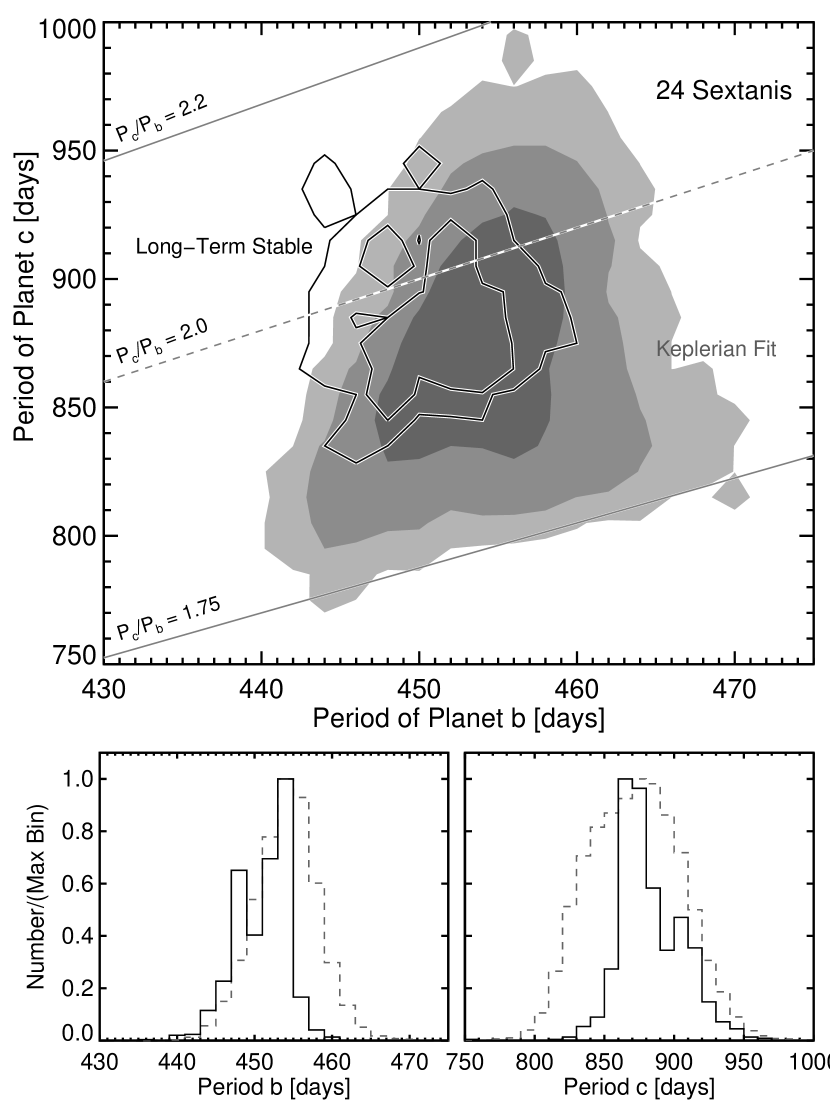
Figure 3.— Top: Comparison of the end-points of the double-Keplerian MCMC analysis (shaded contours), and the n-body DEMCMC analysis with the long-term stable constraint (black, solid contours) for 24 Sex. The contours show the 68.2%, 80% and 95% confidence intervals (inner to outer). To guide the eye, we overlay diagonal lines to indicate 1.75:1, 2:1 & 2.2:1 period ratios. The MCMC posterior sample covers a large range of parameter space and is consistent with a 2:1 period ratio. In contrast, the DEMCMC results are limited to a smaller area of parameter space lying on, or close to, the 2:1 period ratio. Bottom: Histograms for the same planetary period data from 24 Sex, comparing the results from the Keplerian MCMC analysis (black), N-Body DEMCMC analysis (dark gray). When compared to the basic MCMC results, the DEMCMC results for the inner planet are shifted more towards lower periods, while the outer planet shifts towards higher periods, making the overall period ratio converge more closely towards 2:1.

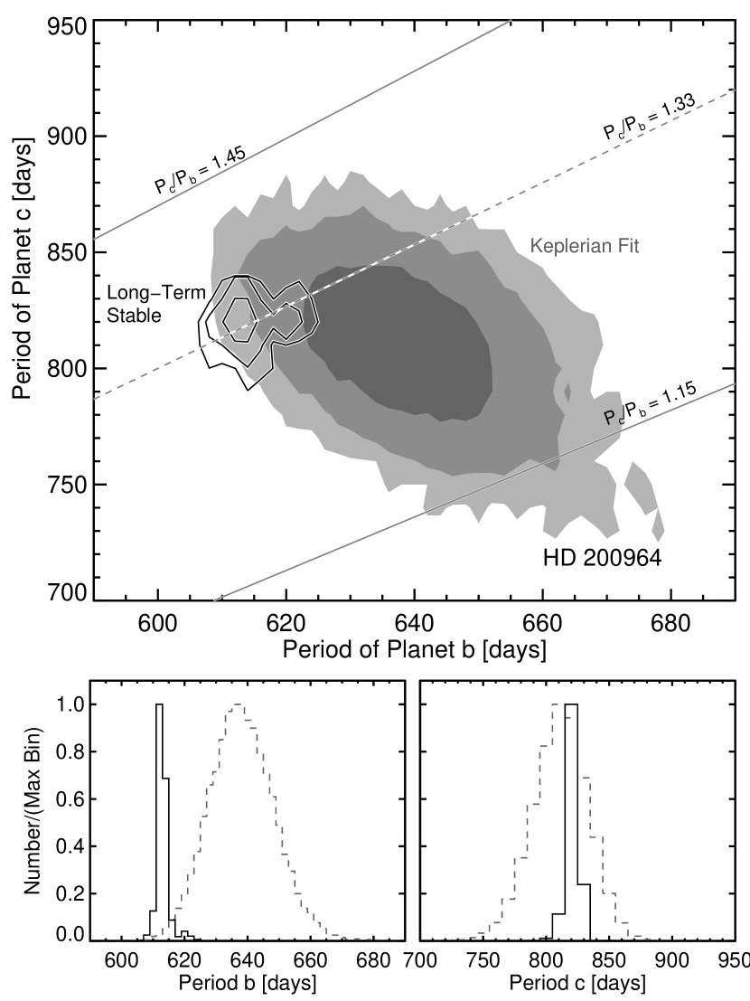
Figure 4.— Top: Comparison of the end-points of the double-Keplerian MCMC analysis (shaded contours), and the n-body DEMCMC analysis with the long-term stable constraint (black, solid contours) for 24 Sex. The contours show the 68.2%, 80% and 95% confidence intervals (inner to outer). To guide the eye, we overlay diagonal lines to indicate 1.15:1, 4:3 & 1.45:1 period ratios. The MCMC posterior sample covers a large range of parameter space and is consistent with a 4:3 period ratio. In contrast, the DEMCMC results are limited to a smaller area of parameter space straddling the 4:3 period ratio. Bottom: Histograms for the two planetary periods in the HD 200964 system, comparing the results from the Keplerian MCMC analysis (black) and N-Body DEMCMC analysis (dark gray). When compared to the basic MCMC results, the DEMCMC results in a decrease in the fitted period of the inner planet, making the overall period ratio converge more closely towards 4:3.

6.3. Numerical Integrations for HD 200964

The results of our n-body DEMCMC simulations for HD 200964 are again more tightly confined than the results of the double-Keplerian analysis. As an example of this we illustrate in Fig. 4 the difference in the end-points of the two analyses, showing a scatter plot of the planetary periods at the end of both the Keplerian analysis and the n-body analysis, as well as histograms for the same data. Again, we note that the shift to an N-Body analysis acts to concentrate the preferred region into a smaller area, while the stability requirements act to shift the favored parameters closer toward the 4:3 period commensurability.

As for the case of 24 Sex, we have applied our DEMCMC method multiple times using numerous randomized initial conditions. Again, we find qualitatively similar results from all sets of the DEMCMC analysis, but with some indication that the results have not truly converged. As such, we interpret these results as demonstrative that stable systems exist which can fit the RV data, and moreover, the extremely narrow range of period ratios favored by the analysis ($\sim 1.32$ to $\sim 1.36$) shows that the current observations strongly favor orbital solutions in or close to the 4:3 MMR.

Next, we test the long-term orbital stability of the orbital solutions identified by the DEMCMC analysis. For HD 200964, $>90\%$ of the systems are clearly unstable during a $10^{7}$ year integration (i.e., they experience a collision or a change in semimajor axes of more than 50%.) We find that $\sim~{}1,000$ of the 16,000 simulations remain stable for $10^{7}$ years. We interpret these as plausible orbital solutions consistent with the RV observations of HD 200964.

As illustrated in Fig. 4, the stable systems occupy a region of parameter space corresponding to a region of paramter space near the 4:3 period ratio. Taking only these long-term stable systems into account, we find that the inner planet has a period $P_{b}=$ 613.8${}^{+1.3}_{-1.4}$ days, semimajor axis $a_{b}=$ 1.601${}^{0.002}_{-0.002}$ AU, eccentricity $e_{b}=$ 0.04${}^{+0.04}_{-0.02}$ and mass $M_{b}\sin{i}=$ 1.85${}^{+0.14}_{-0.08}$ $M_{\rm Jup}$, while the outer planet has a period $P_{c}=$ 825.0${}^{+5.1}_{-3.1}$ days, semimajor axis $a_{c}=$ 1.95${}^{+0.008}_{-0.005}$ AU, eccentricity $e_{c}=$ 0.181${}^{+0.024}_{-0.017}$ and mass $M_{c}\sin{i}=$ 0.90${}^{+0.12}_{-0.06}$ $M_{\rm Jup}$. We detail all the fitted parameters from this analysis in Table 3.

We find that most of the stable planetary orbits overlap, producing strongly interacting systems, resulting in significant oscillations in the the semimajor axes and the eccentricities of both planets. An example stable solution exhibits observable eccentricity oscillations ($0.03<e_{b}<0.1$ and $0.13<e_{c}<0.18$) on an approximately 250-year timescale and semimajor axis oscillations ($1.57<a_{b}<1.58$ and $1.9<a_{c}<1.93$) on an approximately 60 year timescale. Again, as in the 24 Sex system, all of the long-term stable systems examined here for HD 200964 seem to be circulating rather librating. As in the 24 Sex analysis, we find a jitter value of 8.23${}^{+0.38}_{-0.88}$m s^-1, which is larger than the empirical jitter estimate of johnson10b.

7. Summary and Discussion

Our RV measurements of the intermediate-mass subgiants 24 Sex and HD 200964 ($M_{\star}=$ 1.54 and 1.44 $M_{\odot}$, respectively) reveal the presence of a pair of giant planets around each star. Our orbital analysis indicates that most, if not all, of the dynamically stable solutions include crossing orbits, suggesting that each system is locked in a mean motion resonance that prevents close encounters and provides long-term stability. The planets in the 24 Sex system likely have a period ratio near 2:1, while the HD 200964 system is even more tightly packed with a period ratio close to 4:3.

In both the 24 Sex and HD 200964 systems, the planets reside well within the so-called snow line, beyond which volatiles in the protoplanetary disk can condense to provide the raw materials for protoplanetary core growth. For a pre-main-sequence, 1.5 $M_{\odot}$ star the snow line is located beyond 2-3 AU according to the estimates of kennedy08 for realistic disk models including irradiation and accretional heating. It is therefore likely that the planets around 24 Sex and HD 200964 formed at larger semimajor axes and subsequently experienced inward orbital migration (See migrationrev, for a review of migration theory).

Unless the planets around 24 Sex and HD 200964 formed with period ratios close to their current values, the two planets in each system likely migrated through disk interactions at convergent rates until they became trapped in an MMR, with the strong 2:1 resonance being the most likely endpoint of such differential migration (kley00; nelson02). The rarity of planets discovered with period ratios smaller than 2:1 accords well with the dynamical simulations of lee09. In their simulation they considered the formation of two giant planets in a protoplanetary disk with initial period ratios just outside of 2:1 and final orbital configurations determined by the initial conditions and details of the planet-planet-disk interactions. From their ensemble of simulated planetary systems they found that only 3% attain period ratios closer than 2:1, and none ended in stable configurations closer than 3:2.

The ability of planets to reach a resonance tighter than 3:2 is dependent upon a number of factors including the initial separation of the planets, disk viscosity, planet masses, remaining disk mass and size of the gaps opened by the planets (malhotra93; nader99; bryden00; snellgrove01). One key variable is the convergent migration rate, which if fast enough can carry the planets past the deep 2:1 MMR into tighter commensurabilities. The 24 Sex system is near the 2:1 resonance, which may be a reflection of a slower migration process compared to that which led to the extremely tight 4:3 configuration in the otherwise very similar HD 200964 system.

pap10 explored rapid migration scenarios leading to the attainment of high-order MMRs by low-mass planets migrating withing a gas disk. For the terrestrial planets they considered, MMRs with degrees as high as 8:7 and 11:10 were achieved for migration timescales of order $10^{3}$ years. However, to test whether such conditions can lead to high-order stable MMRs for the planets in the HD 200964 system, and the 2:1 MMR seen in the 24 Sex system, hydrodynamic considerations need to be incorporated into the models. rein10 investigated the formation and evolution of the gas giants orbiting HD 45364 and found plausible models for the attainment of the 3:2 MMR observed in that system. Simulations of this nature are beyond the scope of the present work and will be presented in a future contribution (Payne et al. 2010, in prep). For now, it is clear that just like the resonant planetary systems discovered before them, the 24 Sex and HD 200964 systems pose interesting challenges to theories of planet formation and orbital evolution.

Table 4Radial Velocities for 24 Sextanis

JD	RV	Uncertainty	Telescope
-2440000	(m s-1)	(m s-1)
13405.936	-34.98	4.24	L
13435.836	-37.40	4.05	L
13502.774	3.04	3.76	L
13517.768	8.07	3.90	L
13719.011	-13.68	3.46	L
14131.051	38.40	4.17	L
14133.931	37.92	3.49	L
14146.787	28.17	4.15	L
14150.947	34.70	6.03	L
14168.823	28.25	4.33	L
14169.860	30.86	3.65	L
14178.699	36.12	4.10	L
14216.839	-6.66	4.22	L
14218.709	-8.74	6.44	L
14232.713	-4.29	4.05	L
14254.688	-24.93	6.01	L
14255.689	-33.28	4.29	L
14266.699	-25.63	4.77	L
14269.695	-28.99	5.87	L
14274.719	-31.09	4.86	L
14378.045	-24.52	6.79	L
14402.054	2.53	5.26	L
14433.046	24.41	5.29	L
14445.938	4.46	3.08	L
14458.050	4.53	4.31	L
14482.959	11.65	3.89	L
14504.855	8.92	3.36	L
14525.946	25.65	4.37	L
14548.900	22.38	3.29	L
14572.872	13.31	4.54	L
14573.724	16.22	3.77	L
14617.764	11.34	5.29	L
14620.705	-1.69	3.78	L
14621.716	11.26	5.22	L
14627.708	11.39	3.87	L
14650.692	-2.99	6.79	L
14762.024	-24.44	7.00	L
14786.078	-13.05	6.03	L
14806.150	-22.03	1.98	K
14807.075	-18.78	1.83	K
14808.057	-13.83	1.96	K
14809.069	-21.81	1.88	K
14810.149	-15.43	1.88	K
14811.122	-12.80	1.65	K
14847.038	3.99	1.80	K
14847.048	18.53	3.83	L
14904.830	52.37	4.91	L
14929.814	59.40	1.63	K
14955.878	69.74	1.60	K
14963.915	68.12	1.49	K
14978.706	55.29	4.31	L
14983.770	64.81	1.59	K
14984.827	48.72	1.53	K
14987.759	63.15	1.54	K
14988.750	63.85	1.60	K
15002.711	55.03	6.40	L
15014.741	57.09	1.72	K
15015.750	61.18	1.58	K
15151.052	-23.66	6.04	L
15164.112	-21.86	1.83	K
15172.150	-26.29	2.05	K
15173.097	-31.15	1.93	K
15189.119	-40.47	1.85	K
15229.007	-30.27	3.76	L
15241.871	-40.78	4.23	L
15242.872	-36.26	3.75	L
15243.855	-43.99	5.27	L
15260.941	-26.13	1.65	K
15271.797	-27.09	3.77	L
15272.789	-11.58	6.00	L
15273.750	-25.81	3.66	L
15285.854	-12.17	1.75	K
15311.810	-5.48	1.43	K
15312.791	2.81	1.56	K

Table 5Radial Velocities for HD 200964

JD	RV	Uncertainty	Telescope
-2440000	(m s-1)	(m s-1)
13213.895	11.40	4.20	L
13255.775	29.55	3.72	L
13327.604	36.56	3.70	L
13576.944	-20.58	3.98	L
13619.810	-36.28	3.71	L
13641.795	-27.30	3.61	L
13669.629	-18.07	3.55	L
13710.605	-4.99	3.77	L
13894.977	-3.08	3.71	L
13895.921	6.24	3.30	L
13896.963	5.08	3.47	L
13921.953	9.72	3.59	L
13959.788	7.02	3.96	L
14216.976	-19.74	4.09	L
14232.936	-26.06	4.83	L
14244.907	-27.39	5.19	L
14254.960	-16.97	3.70	L
14274.916	-7.88	3.72	L
14288.888	-3.15	3.49	L
14304.877	8.18	4.89	L
14309.845	-1.57	4.28	L
14336.881	16.00	4.49	L
14377.773	10.58	5.74	L
14399.752	33.36	1.62	K
14401.749	41.83	5.67	L
14405.700	39.39	4.02	L
14427.588	35.30	4.29	L
14427.757	25.14	1.18	K
14429.621	49.55	4.41	L
14432.653	30.85	4.89	L
14445.624	23.13	4.22	L
14536.053	20.85	5.26	L
14551.019	25.15	7.90	L
14585.990	22.22	4.51	L
14603.126	14.71	1.39	K
14604.012	18.01	1.58	K
14612.988	-7.49	6.44	L
14621.965	3.21	5.14	L
14622.995	-5.37	4.16	L
14634.079	10.67	1.52	K
14640.923	-1.39	3.34	L
14650.960	-13.59	3.79	L
14656.902	0.00	7.81	L
14674.916	-16.16	1.39	K
14675.850	-16.06	4.87	L
14676.879	-25.35	4.49	L
14677.922	-28.67	3.69	L
14683.850	-22.03	4.24	L
14699.804	-14.57	5.28	L
14734.713	-29.88	3.82	L
14737.790	-29.53	5.34	L
14738.751	-36.28	4.54	L
14747.711	-59.70	3.80	L
14766.659	-48.87	3.96	L
14778.803	-45.21	1.61	K
14785.605	-51.33	4.06	L
14790.734	-47.17	1.34	K
14807.789	-46.94	1.60	K
14935.136	-18.39	1.16	K
14941.012	-18.06	6.19	L
14941.989	-24.98	4.38	L
14956.097	-14.88	1.50	K
14964.120	-5.85	1.33	K
14978.935	-3.81	5.48	L
14984.070	6.28	1.43	K
14985.095	4.20	1.62	K
14986.112	-1.27	1.71	K
14987.129	3.06	1.39	K
14989.069	6.64	1.33	K
15002.947	32.46	5.34	L
15014.972	22.36	1.54	K
15015.957	11.56	1.44	K
15027.007	22.52	1.55	K
15042.973	33.72	1.69	K
15049.001	42.16	1.62	K
15060.816	45.09	4.29	L
15061.819	45.31	3.69	L
15062.829	47.93	3.69	L
15075.078	45.22	1.68	K
15076.067	43.59	1.75	K
15077.056	49.98	1.57	K
15082.047	45.65	1.53	K
15083.053	52.10	1.63	K
15084.028	55.68	1.57	K
15085.004	46.81	1.60	K
15091.772	64.86	4.56	L
15092.725	57.80	3.96	L
15106.911	57.25	1.51	K
15123.798	55.22	4.81	L
15135.755	48.13	1.43	K
15148.734	61.20	4.57	L
15150.620	54.74	5.97	L
15187.695	44.10	1.66	K
15188.688	41.49	1.69	K
15290.146	11.79	1.39	K
15313.137	2.22	1.33	K

Table 6Summary of Photometric Observations From Fairborn Observatory

Program	Comparison	Comparison	Date Range	Duration		$\sigma{(P-C1)}_{by}$	$\sigma{(P-C2)}_{by}$	$\sigma{(C2-C1)}_{by}$
Star	Star 1	Star 2	(HJD $-$ 2,400,000)	(days)	$N_{obs}$	(mag)	(mag)	(mag)	Variability
(1)	(2)	(3)	(4)	(5)	(6)	(7)	(8)	(9)	(10)
24 Sex	HD 87974	HD 89734	54438–55333	895	243	0.0022	0.0020	0.0020	Constant
HD 200964	HD 201507	HD 201982	54578–55167	589	100	0.0015	0.0014	0.0015	Constant