Vertical Structure and Turbulent Saturation Level in Fully Radiative Protoplanetary Disc Models

Abstract

We investigate a massive ($\varSigma\sim 10\,000\mbox{ g}\,\mbox{cm}^{-2}$ at 1 AU) protoplanetary disc model by means of 3D radiation magnetohydrodynamics simulations. The vertical structure of the disc is determined self-consistently by a balance between turbulent heating caused by the MRI and radiative cooling. Concerning the vertical structure, two different regions can be distinguished: A gas-pressure dominated, optically thick midplane region where most of the dissipation takes place, and a magnetically dominated, optically thin corona which is dominated by strong shocks. At the location of the photosphere, the turbulence is supersonic ($M\sim 2$), which is consistent with previous results obtained from the fitting of spectra of YSOs. It is known that the turbulent saturation level in simulations of MRI-induced turbulence does depend on numerical factors such as the numerical resolution and the box size. However, by performing a suite of runs at different resolutions (using up to 64x128x512 grid cells) and with varying box sizes (with up to 16 pressure scaleheights in the vertical direction), we find that both the saturation levels and the heating rates show a clear trend to converge once a sufficient resolution in the vertical direction has been achieved.

1 Introduction & Motivation

Despite many years of observational and theoretical research, the physics of protoplanetary accretion discs is still not well understood. Significant uncertainties remain both with respect to their physical composition as well as their temporal evolution. Their rather short lifetime of $\sim 10^{6}\mbox{ to }10^{7}\,\mathrm{yr}$ (Hartmann et al., 1998; Sicilia-Aguilar et al., 2006) requires a physical process that transfers angular momentum outwards efficiently so that the matter can be accreted fast enough onto the star. Usually it is assumed that some sort of turbulence is acting in the disc, providing an effective viscosity that drives accretion (Shakura & Syunyaev, 1973, hereafter SS). As of today, the most promising mechanism for this scenario appears to be the magneto-rotational instability (MRI), a linear instability that exists in rotating, weakly magnetised shear flows and operates under very general conditions (Balbus & Hawley, 1998; Balbus, 2003, 2009).

Apart from protoplanetary discs, the MRI plays an important role also in a variety of other accreting systems, for example accretion discs in active galactic nuclei, galactic accretion discs and core-collapse supernovae. Although these systems cover very different physical regimes, they can be modeled using similar numerical methods. The most common approach is to employ the shearing-box approximation, where one models a small patch of the accreting disc in the co-moving frame using special “shear-periodic” boundary conditions which are consistent with the background shear flow (Hawley et al., 1995, hereafer HGB). The shearing-box model has the advantage that it is easy to set up, and that it is not very expensive computationally. In contrast to the many works that make use of the shearing-box approximation, there are only very few global simulations of protoplanetary discs (Fromang & Nelson, 2009; Flock et al., 2010; Dzyurkevich et al., 2010), all employing an isothermal equation of state.

The most interesting quantity that numerical simulations can provide is the magnitude of the turbulent viscosity, which is usually measured in terms of the alpha parameter (SS, HGB). Numerical simulations show that the MRI leads to sustained turbulence which transports angular momentum outwards at a rate that, for the case of protoplanetary discs (but maybe not for other systems), is compatible with observations (King et al., 2007). The saturation level of the MRI depends on numerical parameters such as the box size (Johansen et al., 2009), the numerical resolution (Fromang & Papaloizou, 2007; Simon et al., 2009; Davis et al., 2009; Shi et al., 2010, herafter SKH) and the numerical scheme (Balsara & Meyer, 2010). There is also a dependence on the physical parameters viscosity and resisistivity (Fromang et al., 2007) and, to a lesser extent, also on the thermodynamics (Flaig et. al. 2009, herafter FK2; see also Turner et. al. 2003). When doing MRI simulations, it is therefore very important to check the dependence of the results on numerical factors and also to include as much of the relevant physics as possible.

Protoplanetary discs are dense systems and therefore for a large part optically thick. This means that one should include radiation transport in order to properly model the transport of radiation energy from the disc midplane, which is constantly heated by turbulent dissipation, to the upper layers, where the radiation escapes into space. Including radiation transport is very important in order to get the correct vertical structure, which will be determined by a dynamic balance between turbulent heating and radiative cooling. It is also an important step towards the goal of comparing numerical simulations to actual observations by modelling accretion disc spectra, and thereby deriving constraints on physical parameters.

While such an attempt to include radiation transport in MRI-turbulent protoplanetary disc simulations has not been reported so far, there exist already several works which include radiative transfer in simulations of accretion discs that are situated in other physical regimes (for example Turner, 2004; Krolik et al., 2007, for the case of radiation dominated discs). The gas-pressure dominated simulation of  Hirose et al. (2006), hereafter HKS, is most closely related to our work, and will be the main source of reference. In such simulations it is possible to track in quite some detail the path that the energy takes inside accretion discs (HKS) and it is possible to derive observable consequences (Blaes et al., 2006).

When dealing with protoplanetary discs one has to consider that these are not only dense, but also cold, which means that for a large part they will only be poorly ionised, leading to the formation of a “dead zone” (Gammie, 1996). The effects of a finite resistivity have already been studied in isothermal models (for example Sano et al., 2000; Turner & Sano, 2008; Dzyurkevich et al., 2010). In the present work, we avoid this additional complication by placing our simulation domain near to the star and choosing a surface density that is high enough so that the turbulent heating provides a sufficient amount of collisional ionisation, thereby justifying the assumption of ideal MHD. In a later work, we will extend our model by including a physical resisitvity, thereby arriving at a protoplanetary disc model that includes all the relevant physics in a self-consistent manner.

The organisation of our paper is as follows: In §2 we describe our numerical methods and the model setup. In §3 the results of our simulations are presented. In §4 we conclude and provide an outlook on the further research that is planned.

2 Model description

We apply the stratified shearing-box approximation, i.e. our simulations take place in a co-moving rectangular box that is small enough so that local Cartesian coordinates $(x,y,z)$ can be introduced, which correspond to the radial, azimuthal and vertical coordinates, respectively. The radial boundary conditions are shear-periodic and the azimuthal boundary conditions are strictly periodic (HGB). In the vertical direction we apply open boundary conditions that allow outflow, but no inflow. The simulation box is placed at a distance of $1\,{\rm AU}$ from the central star which has one solar mass. We choose a surface density $\varSigma_{0}$ of order $\sim 10\,000\,\,{\rm g\,cm^{-2}}$, which lies in between the value of $\varSigma_{0}=1700\,\,{\rm g\,cm^{-2}}$ given by the minimum mass solar nebula of Hayashi (1981) and the value of $\varSigma_{0}=50500\,\,{\rm g\,cm^{-2}}$ according to the more recently proposed solar nebula model by Desch (2007). With this choice of surface density, the temperatures that come out of our model are of the order of $1000-2000\,\mathrm{K}$ in the body of the disc, which allows us to describe the the disc gas using the ideal MHD equations. The gas is assumed to have solar chemical composition, therefore we choose values of $\gamma=1.4$ for the adiabatic index and $\mu=2.35$ for the mean molecular weight.

For protoplanetary discs, the stellar irradiation plays an important role in determining the degree of ionisation in the disc, because stellar X-rays are one of the main ionisation sources. However, since for our choice of parameters the disc can be considered to be already sufficiently ionised for the MRI to work, we may safely neglect this factor. At visible wavelengths, the stellar irradiation will only be important in the very upper layers of a protoplanetary disc, where according to passively heated models, a temperature inversion will occur (Chiang & Goldreich, 1997). In the present work we are mainly interested in the temperature profile as it results from a balance between active heating by turbulent dissipation and cooling by radiation transport. Therefore we exclude this region from our simulation domain and neglect the stellar irradiation in the visible part of the spectrum also. For reference, the basic properties of our model are summarised in Table 1.

Parameter	Symbol	Value
Radial box size	$L_{x}$	${\rm 0.08\,AU}$
Azimuthal box size	$L_{y}$	${\rm 0.48\,AU}$
Vertical box size	$L_{z}$	${\rm 0.8\,AU}$ - ${\rm 1.28\,AU}$
Mass of central star	$M_{\ast}$	$1\,M_{\odot}$
Distance to central star	$R_{0}$	${\rm 1\,AU}$
Surface density	$\varSigma_{0}$	${\rm 11\,356\,\,g\,cm^{-2}}$
Adiabatic index	$\gamma$	$1.4$
Mean molecular weight	$\mu$	$2.35$

Table 1: Summary of basic physical parameters of our model. The vertical box size of $L_{z}=0.8\,{\rm AU}$ corresponds to a model which covers 10 pressure scale heights in the vertical direction, while $L_{z}=1.28\,{\rm AU}$ corresponds to a model with 16 scale heights.

2.1 Equations solved

We calculate the dynamics of the disc gas by solving the equations of radiation magnetohydrodynamics in conservative form. We make the one-temperature approximation (i.e. we assume thermal equilibrium between matter and radiation), which means that we need not to solve an additional equations for the radiation energy. Radiative diffusion is treated within the flux-limited diffusion approach. Including the source terms that arise in shearing box framework, the resulting set of equations looks as follows:

$$\frac{\partial\rho}{\partial t}+\bm{\nabla}\cdot(\rho\bm{v})=0,$$ (1a)

$$\frac{\partial(\rho\bm{v})}{\partial t}+\bm{\nabla}\cdot\left(\rho\bm{v}\bm{v}+P_{\mathrm{tot}}\mathsf{I}-\frac{\bm{B}\bm{B}}{4\uppi}\right)=\bm{f},$$ (1b)

$$\frac{\partial E_{\mathrm{tot}}}{\partial t}+\bm{\nabla}\cdot\left[(E_{\mathrm{tot}}+P_{\mathrm{tot}})\bm{v}-\frac{\bm{B}(\bm{B}\cdot\bm{v})}{4\uppi}\right]=\bm{f}\cdot\bm{v}-\bm{\nabla}\cdot\bm{F},$$ (1c)

$$\frac{\partial\bm{B}}{\partial t}-\bm{\nabla}\times(\bm{v}\times\bm{B})=0;$$ (1d)

where the total pressure $P_{\mathrm{tot}}=p+B^{2}/8\uppi$ is the sum of gas pressure and magnetic pressure (neglecting the contribution arising from radiation pressure), $\mathsf{I}$ is the identity matrix, $\bm{f}$ denotes the sum of the gravitational forces and the inertial forces arising in the shearing-box system, $E_{\mathrm{tot}}=p/(\gamma-1)+\rho v^{2}/2+B^{2}/8\uppi+E_{\mathrm{rad}}$ is the total energy, $\bm{F}=-(\lambda c/\kappa\rho)\bm{\nabla}E_{\mathrm{rad}}$ is the radiative energy flux, and the other symbols have their usual meaning. Using linearised expressions for the gravitational and inertial forces, $\bm{f}$ becomes (HGB):

$$\bm{f}=3\rho\varOmega^{2}x\,\hat{\bm{x}}-\rho\varOmega^{2}z\,\hat{\bm{z}}+2\rho\varOmega\bm{v}\times\hat{\bm{z}},$$ (2)

with $\varOmega$ the angular orbital frequency. Note that by solving the total energy equation, rather than the thermal energy equation, all dissipative losses are automatically captured and transformed into gas internal energy. In this way the heating of the gas is consistent with the dissipation caused by the turbulence.

In the optically thick protoplanetary discs, matter and radiation are closely coupled and we can assume that they are at the same temperature, which means that the radiation energy density is given by $E_{\mathrm{rad}}=aT^{4}$, which closes our system of equations. For the flux limiter $\lambda$ we apply the formula given in Eq. (28) of Levermore & Pomraning (1981).

Figure 1: Opacity as a function of temperature and density. The thick curve gives the opacities for the typical densities and temperatures found in our model R7, where M and S correspond to the location of the midplane and the surface, respectively, while the star $\star$ denotes the mean location of the photosphere. For an explanation of the different opacity regions ➀ to ➃ see the text.

We use dust opacities $\kappa=\kappa(\rho,T)$ as described in Bell & Lin (1994), which are calculated as a function of the gas density and temperature. Fig. 1 shows a plot of the opacity function for the typical density and temperature range that we have in our simulations. Four different regions can be distinguished: At the lowest temperatures, in region ➀, the dominant contribution to the opacity is due to ice grains. Since these are more efficient scatterers and absorbers at shorter wavelengths, the opacity increases with temperature. In region ➁, ranging from $\sim 170$ to $\sim 200\,{\rm K}$, the ice grains melt, so the opacity decreases. Region ➂ is dominated by dust grains and the opacity shows only a weak temperature dependence of the form $\kappa\propto T^{0.5}$. Finally, in region ➃, the temperatures and densities are sufficiently high for the dust grains to start melting, leading again to a decrease of the opacity.

2.2 Numerical code

We use the Cronos magnetohydrodynamics code (Kissmann et al., 2008). The code has already been successfully applied to simulations of the turbulent interstellar medium (Kissmann et al., 2008), coronal mass ejections (Pomoell et al., 2008) and simulations of MRI turbulence in accretion discs (FK2). The code solves the ideal MHD equation using the conservative scheme described in Kurganov et al. (2001). Since we do not include any explicit dissipation, the turbulent cascade is cut off at the grid scale, where kinetic and magnetic energy are lost due to numerical errors and transformed into gas internal energy by virtue of the conservative properties of the underlying numerical scheme. The fact that the heating is mainly due to numerical effects means that there will inevitably be some dependence on numerical parameters such as the resolution and the details of the numerical scheme involved. However, since numerical errors are largest at locations where there are sharp gradients in velocity and magnetic field, the numerical dissipation should at least qualitatively resemble the actual physical dissipation (HKS, Krolik et al., 2007). For high enough resolutions, we expect the results to become independent of numerical parameters. It is therefore very important to perform runs at different resolutions in order to check that the results are actually converged.

The radiation transport is treated using operator splitting. During the radiation transport step, the equation $\partial(e_{\mathrm{th}}+E_{\mathrm{rad}})/\partial t=-\bm{\nabla}\cdot\bm{F}$ is solved, which, using the relations $e_{\mathrm{th}}=\rho k_{\mathrm{B}}T/(\gamma-1)\mu m_{\mathrm{H}}$ and $E_{\mathrm{rad}}=aT^{4}$, can be transformed into the following diffusion equation for the temperature:

$$(c_{\mathrm{V}}\rho+4aT^{3})\frac{\partial T}{\partial t}=\bm{\nabla}\cdot\frac{\lambda c}{\kappa\rho}4aT^{3}\bm{\nabla}T,$$ (3)

where $c_{\mathrm{V}}=k_{\mathrm{B}}/(\gamma-1)\mu m_{\mathrm{H}}$. In order to avoid prohibitively short timesteps due to the presence of optically thin regions, Eq. (3) is solved implicitly (for more details on the implementation of the radiation transport, see the appendix).

2.3 Boundary & initial conditions

Name	Resolution	Box size	grid cells/$H_{0}$	Orbits	TD	$\langle\langle\alpha_{\mathrm{Reyn}}\rangle\rangle$	$\langle\langle\alpha_{\mathrm{Maxw}}\rangle\rangle$	$\langle\langle\alpha\rangle\rangle$
I6	32x64x256	$H_{0}\times 6H_{0}\times 12H_{0}$	21	200	isothermal	$0.001\pm 0.001$	$0.003\pm 0.004$	$0.004\pm 0.005$
I5	32x64x256	$H_{0}\times 6H_{0}\times 10H_{0}$	25	80	isothermal	$0.003\pm 0.002$	$0.011\pm 0.006$	$0.014\pm 0.008$
I7	32x64x448	$H_{0}\times 6H_{0}\times 14H_{0}$	32	70	isothermal	$0.004\pm 0.001$	$0.013\pm 0.003$	$0.017\pm 0.004$
I6D	64x128x512	$H_{0}\times 6H_{0}\times 12H_{0}$	42	60	isothermal	$0.003\pm 0.001$	$0.012\pm 0.005$	$0.015\pm 0.006$
R6	32x64x256	$H_{0}\times 6H_{0}\times 12H_{0}$	21	200	radiative	$0.001\pm 0.001$	$0.004\pm 0.003$	$0.005\pm 0.004$
R7	32x64x448	$H_{0}\times 6H_{0}\times 14H_{0}$	32	150	radiative	$0.003\pm 0.002$	$0.015\pm 0.010$	$0.018\pm 0.013$
R8	32x64x512	$H_{0}\times 6H_{0}\times 16H_{0}$	32	90	radiative	$0.004\pm 0.002$	$0.018\pm 0.009$	$0.022\pm 0.011$
R6D	64x128x512	$H_{0}\times 6H_{0}\times 12H_{0}$	42	60	radiative	$0.004\pm 0.002$	$0.017\pm 0.008$	$0.021\pm 0.010$

Table 2: Overview of the simulation runs that were performed. The box size (third column) is measured in scaleheights $H_{0}$ refering to the initial gas pressure at the midplane. Since the pressure at the midplane does not change very much, this corresponds very well to the actual pressure scaleheight during the simulation. The fourth column gives the number of grid cells per scale height in the vertical direction. The fifth column tells the number of orbits for which the simulation has been run. “TD” (sixth column) denotes the the type of thermodynamics. The last three columns contain the time-averaged values of the turbulent stresses as well as the standard deviation.

In the radial direction, shear-periodic boundary condtions are applied, which are consistent with the shear flow in our local box (HGB). The azimuthal boundary conditions are periodic. In the vertical direction, we use outflow boundary conditions which extrapolate the values of the density and the velocity in the outermost cell into the ghost zones. In order to prevent inflow of mass, reflective boundary conditions are applied instead whenever the velocity vector points into the computational domain. For the magnetic field, we apply vertical field boundary conditions, where $B_{x}$ and $B_{y}$ are set to zero in the ghost cells and $B_{z}$ is extrapolated from the outermost computational cell. With this set-up we do not need any (artificial or physical) resistivity near the boundaries in order to prevent inconvenient effects. At the boundaries, the temperature is set to a small fixed value of $T_{\mathrm{b}}={\rm 10\,K}$, which is kept constant throughout the simulation. This prescription for the temperature allows for free emission of the radiation from the disc surface, and it is well justified by the fact that in our models the gas at the boundary is always optically thin.

As the initial condition we choose a state of approximate vertical hydrostatic equilibrium:

$$\begin{array}[]{rcl}\rho(t=0)&=&\rho_{\mathrm{m}}\exp(-z^{2}/2H_{0}^{2}),\\ \bm{v}(t=0)&=&\bm{v}_{\mathrm{kep}}+\delta\bm{v},\\ T(t=0)&=&T_{0},\\ B(t=0)&=&\bm{\nabla}\times\delta\bm{A},\end{array}$$ (4)

with the scale height $H_{0}=c_{\mathrm{g0}}/\varOmega$, where $c_{\mathrm{g0}}=\sqrt{kT_{\mathrm{0}}/\mu m_{\mathrm{H}}}$ is the initial gas sound speed, and $\bm{v}_{\mathrm{kep}}=-\frac{3}{2}\varOmega x\,\hat{\bm{y}}$ is the background Keplerian shear flow. For the initial midplane density $\rho_{\mathrm{m}}$ and the initial temperature $T_{\mathrm{0}}$ we choose the values $\rho_{\mathrm{m}}={\rm 3.93\cdot 10^{-9}\,g\,cm^{-3}}$ (corresponding to a midplane number density $n_{\mathrm{m}}=10^{15}\,{\rm cm^{-3}}$) and temperature $T_{\mathrm{0}}={\rm 1500\,K}$, respectively. The surface density is then $\varSigma_{0}={\rm 11356\,g\,cm^{-2}}$. In order to avoid excessive shrinking or swelling of the disc during the inital phase, the initial temperature $T_{0}$ has been chosen (by trial and error) such that it is roughly the midplane temperature that comes out of the simulations for this particular combination of $\varSigma_{0}$ and $R_{0}$. Small random perturbations $\delta\bm{v}$ of order $10^{-3}\,c_{\mathrm{g0}}$ are added to the velocity. Finally, the initial magnetic field is derived from the following vector potential:

$$\delta\bm{A}=B_{0}\frac{\sin(2\uppi x/L_{x})}{2\uppi/L_{x}}\,\exp(-z^{2}/2H_{0}^{2})\,\hat{\bm{y}}.$$ (5)

Note that the initial net magnetic flux in the computational domain is thus zero, and this property is retained throughout the simulation to good accuracy. The value of $B_{0}$ is taken such that it corresponds to a plasma beta of $\beta=100$ at the midplane. With this particular choice of magnetic field, the whole disc quickly becomes turbulent in less than 10 orbits.

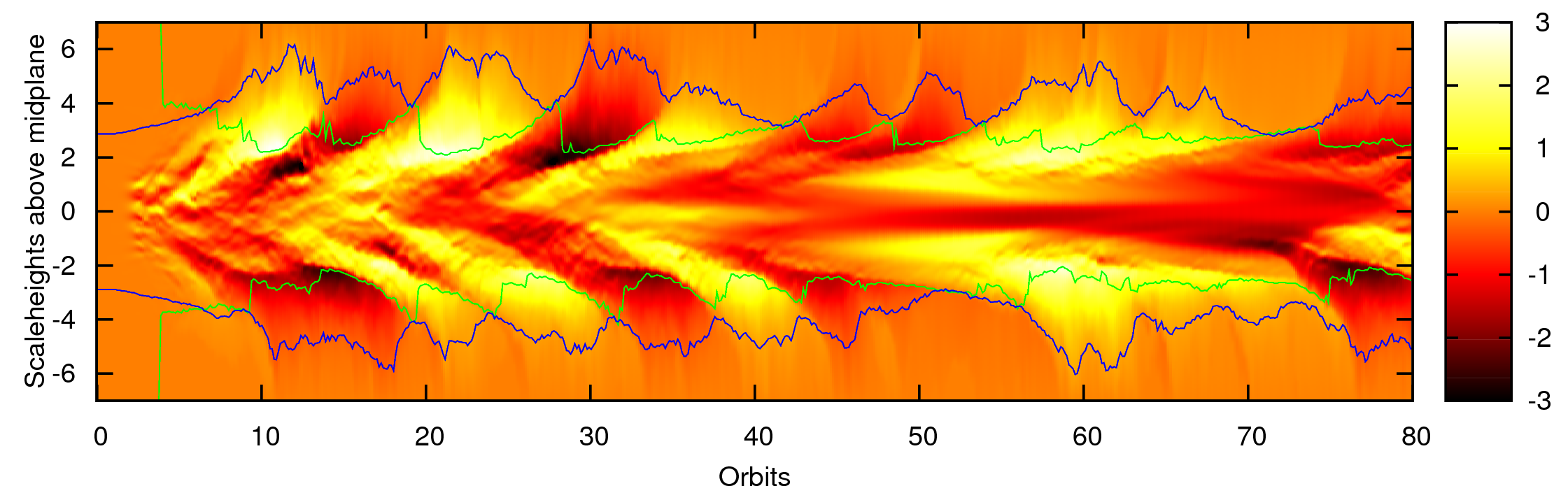
(a) Horizontally averaged azimuthal magnetic field component $B_{y}$ normalised to the initial magnetic field strength $B_{0}$. The blue curve denotes the location of the photosphere and the green curve is the location at which magnetic pressure starts to exceed gas pressure.

(b) Volume averaged magnetic, turbulent kinetic and thermal energy normalised to the initial gas pressure at the midplane. The gas internal energy is about 100 times the magnetic energy (note the different scaling).

(c) Volume averaged turbulent stresses normalised to the mean gas pressure.

(d) Photospheric temperature at top and bottom boundary.

Figure 2: Time history of various physical variables for model R7 from 0 to 80 orbits illustrating the changes in turbulent activity and the correlations between stresses, magnetic field strength and luminosity of the disc. For further explanation see the text.

2.4 Definition of mean quantities

Since we want to investigate the vertical structure of the disc, we are especially interested in horizontally averaged quantities. Therefore, for any quantity $q$, we define the radially and azimuthally averaged value $\langle q\rangle_{xy}$ as

$$\langle q\rangle_{xy}=\frac{1}{L_{x}L_{y}}\int\!\!\!\int q\,\mathrm{d}x\,\mathrm{d}y.$$ (6)

In addition to this, we will also use the volume average $\langle q\rangle$, which is defined as

$$\langle q\rangle=\frac{1}{L_{x}L_{y}L_{z}}\int\!\!\!\int\!\!\!\int q\,\mathrm{d}x\,\mathrm{d}y\,\mathrm{d}z.$$ (7)

The definitions (6) and  (7) are of course to be understood in a discretised sense.

The most important factor that determines the disc’s temporal evolution is the amount of angular momentum transport that takes place inside the disc. It is related to the $r-\phi$ component of the total stress (Balbus & Hawley, 1998), which, in the local shearing-box frame, reads

$$T_{xy}=\rho v_{x}\delta v_{y}-\frac{B_{x}B_{y}}{4\uppi},$$ (8)

where $\delta v_{y}=v_{y}+\frac{3}{2}\varOmega x$. $T_{xy}$ can be decomposed as the sum of Reynolds stress $T_{\rm Reyn}=\rho v_{x}\delta v_{y}$ and Maxwell stress $T_{\rm Maxw}=-B_{x}B_{y}/4\uppi$.

Following the $\alpha$ prescription of SS, we normalise the stresses to the mean gas pressure. We thus define the volume-averaged alpha parameter as

$$\langle\alpha\rangle=\langle\alpha_{\mathrm{Reyn}}\rangle+\langle\alpha_{\mathrm{Maxw}}\rangle,$$ (9)

where

$$\langle\alpha_{\mathrm{Reyn}}\rangle=\langle T_{\rm Reyn}\rangle/\langle P\rangle\mbox{ and }\langle\alpha_{\mathrm{Maxw}}\rangle=\langle T_{\rm Maxw}\rangle/\langle P\rangle$$ (10)

are the volume-averaged Reynolds and Maxwell stresses normalised by the mean gas pressure.

3 Simulations

Table 2 provides an overview of the simulations that were performed. We perform simulations with different box sizes and resolutions. The lowest resolution chosen is $32\times 64\times 256$ (Model R6). We also perform a simulation at double the resolution in all directions (simulation R6D) and two simulations (R7 and R8) with a larger box size in the vertical direction and a vertical resolution that is in between model R6 and R6D, since recent results indicate that it is the resolution in the vertical direction that is critical in determining the value of the turbulent saturation level (SKH). In order to see how the results from the radiative simulations compare to simulations which use an isothermal equation of state, we also perform a set of simulations (I5, I6, I7 and I6D) which have identical physical parameters as the radiative simulations but which use an isothermal equation of state where the temperature is constant kept constant at the initial value of $T_{0}$.

3.1 Time history

Starting from the initial state described in Sec. 2.3 the MRI starts to grow quickly and the non-linear state is reached already after a few orbits. After ten orbits the whole disc is fully turbulent and remains turbulent for the whole course of the simulation. Concerning the time history we now concentrate on model R7.

The turbulent state is not time-steady, but there are periods of high turbulent activity which are followed by periods where the disc is less active. This behaviour can be observed in Fig. 2, where various physical quantities are plotted as function of time for the first 80 orbits. Fig. 2(a) shows the horizontally averaged azimuthal component of the magnetic field (which is the dominant component). During an active phase the magnetic field is lifted upwards, leading to the typical butterfly structure. Recently it has been claimed that it is the undulatory Parker instability that drives the updwelling of the magnetic field (SKH). As one can estimate from Fig. 2(a), one cycle lasts between 10 and 20 orbits. Often the changes in turbulent activity are accompanied by magnetic field reversals in one or both sides of the disc. Unlike, for example, the solar butterfly diagram, the field reversals shown in Fig. 2(a) do not follow a regular pattern and there is no strict correlation between the magnetic polarities in both sides of the disc.

In Fig. 2(a) we also plot the location of the photosphere (defined as the location where the optical depth equals unity) and the position of the magnetosphere (defined as the location where the magnetic pressure starts to exceed the gas pressure). Just between two active phases, the locations of the magnetosphere and the photosphere coincide, so the magnetically dominated region is optically thin. During an active phase, the disc expands due to the stronger magnetic forces and the photosphere is pushed outwards. At the same time, the magnetosphere is pushed inwards due to the higher magnetisation caused by stronger turbulence. Therefore, for much of the time, the magnetically dominated region is for a large part optically thick. The same phenomenon has also been reported in the gas-pressure dominated simulation of HKS, although the physical regime is quite different.

We plot the time history of the energies (thermal energy, turbulent kinetic energy and magnetic energy) in Fig. 2(b). During active periods the magnetic energy is much larger then during a quiet period. The turbulent kinetic energy (that is the total kinetic energy minus the kinetic energy of the background shear flow) is also larger during active phases. In contrast to this, the long-term changes in the thermal energy are much smaller than the up-and-down variations, which shows that we have indeed reached thermal equilibrium.

The turbulent stresses that determine the angular momentum transport in the disc are shown in Fig. 2(c). The angular momentum transport is dominated by the Maxwell stress which is about four to six times larger than the Reynolds stress. This ratio is consistent with previous results for stratified boxes (for example Stone et al., 1996). From a comparison between Fig. 2(b) and Fig. 2(c) it is evident that the magnetic energy and the alpha parameter are strongly correlated. Indeed, it is known that in shearing-box calculations, the time-dependence of the alpha parameter can be fitted by a formula of the form $\langle\alpha\rangle\propto\langle B^{2}\rangle+{\rm const.}$ (see Brandenburg, 2008).

Finally, we may ask how the observational appearance of the disc will change due to phases of varying turbulent activity. To address this question, we plot in Fig. 2(d) the photospheric temperature (i.e. the temperature at the location where the optical depth equals unity). If we compare Fig. 2(d) with Fig. 2(c), it is obvious that in general a high degree of turbulent activity leads to a higher flux of radiation through the disc’s boundaries. The increased flux then balances the increased turbulent heating, so that the thermal energy content in the disc remains nearly constant. This observation can be made more quantitative by looking at the cross-correlation between alpha-parameter and photospheric temperature (Fig. 3):

$$C(\tau)=\int[\langle\alpha\rangle(t-\tau)-\langle\langle\alpha\rangle\rangle][T_{\mathrm{phot}}(t)-\langle T_{\mathrm{phot}}\rangle]\,\mathrm{d}t.$$ (11)

Here, $\langle\alpha\rangle$ denotes the volume-averaged alpha parameter as defined in Eq. (9) and $T_{\mathrm{phot}}$ is the arithmetic mean of the photospheric temperatures at top and bottom. The lag $\tau$ between photospheric temperature and alpha parameter (as inferred from the peak in the correlation function) is about 2-3 orbits. We can compare this to the radiative diffusion timescale $\tau_{\mathrm{rad}}=H_{0}^{2}/D_{\mathrm{rad}}$, where the radiative diffusion coefficient $D_{\mathrm{rad}}$ is given by

$$D_{\mathrm{rad}}=4acT^{3}/3c_{\mathrm{V}}\kappa\rho^{2}$$ (12)

(cf. the appendix). When taking typical values $\rho=2.0\cdot 10^{-9}\,\mathrm{g\,cm^{-3}}$ and $T=1700\,\mathrm{K}$ for the density and the temperature in the region near the midplane (see Fig. 5 and Fig. 6 later in the paper), we get $\tau_{\mathrm{rad}}\sim 2.5$ orbits, so the lag between stress and photospheric temperature agrees well with the radiative diffusion timescale. Concerning the turbulent transport coefficient $D_{\mathrm{turb}}=v_{z}^{2}/\varOmega$, we find that near the midplane $D_{\mathrm{turb}}$ is typically about one order of magnitude smaller than $D_{\mathrm{rad}}$, so the energy transport by turbulent gas motions is negligible compared to the energy transport by radiative diffusion.

Figure 3: Cross-correlation between alpha stress and photospheric temperature for model R7.

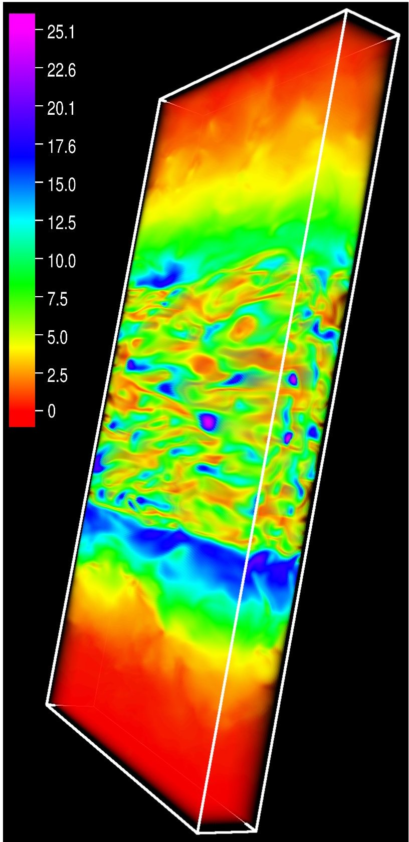
(a) Magnetic field strength $|\bm{B}|$ measured in Gauss.

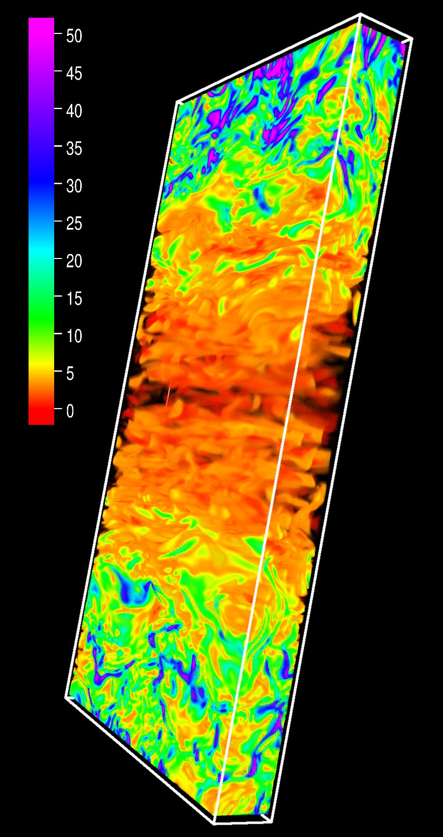
(b) Vorticity $\omega=|\bm{\nabla}\times\bm{v}|$ in units of angular orbital frequency $\varOmega$.

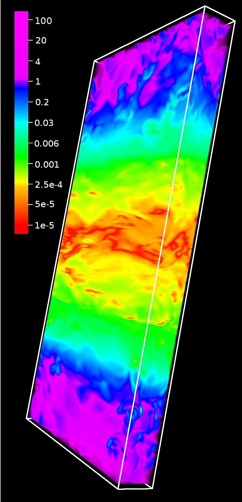
(c) Ratio of photon mean free path to the length over which the temperature varies.

Figure 4: Snapshots from model R6D illustrating the two-layer structure of the disc. The plots in panels (a) and (b) have been taken at $t=20$ orbits, the plot in panel (c) has been taken at $t=21$ orbits. For further comments see the text. (Graphics have been produced using the Vapor visualisation package.)

Figure 5: Temperature profiles obtained for the radiative models. Averages have been taken from 20 orbits until the end of the simulation.

3.2 Vertical structure

To get an impression of how the turbulent state looks like, the reader may first have a look at Fig. 4, where 3D snapshots of some physical quantities are shown for the high-resolution model R6D. Panel (a) depicts the magnetic field strength measured in Gauss. In panel (b) a plot of the vorticity measured in units of the angular orbital frequency $\varOmega$ is shown. Panel (c) contains a plot of the quantity

$$R_{z}=\frac{|\partial_{z}E_{\mathrm{rad}}|}{\kappa\rho E_{\mathrm{rad}}}=\frac{4|\partial_{z}T|}{\kappa\rho T}$$ (13)

which is the ratio of the photon mean free path $\ell_{\mathrm{phot}}=1/\kappa\rho$ to the typical length over which the radiation energy (or the temperature) varies.

Concerning the vertical structure, two regions with very different physical properties can be disinguished: On the one hand, there is the region near the midplane (the region inside the first three scaleheights). Here, the magnetic field is approximately uniform and of the order of several Gauss. The turbulence is subsonic (see Sec. 3.2.3 below) and many intertwined vortices can be observed. Since $R_{z}\ll 1$ the photons are diffusing in this region. On the other hand, there is the corona (the region outwards from 4 scaleheights) which exhibits markedly different features: Here, the magnetic field drops sharply, the flow is supersonic and characterised by strong shocks, and the photons are to a large part better described as free streaming rather than diffusing.

Due to the properties of the shearing-box setup, on average the physical state will appear homogeneous with respect to the radial and the azimuthal direction. This suggests to consider horizontal averages of physical quantities. However, due to the turbulent nature of the flow, the horizontal average of some variable at one instant in time shows large fluctuations and sometimes strong asymmetries between the two halves of the disc. It is therefore necessary to perform averages over many orbits in order to achieve a smooth and symmetric vertical profile.

3.2.1 Density & temperature profile

One of the most interesting quantities that our radiative models are able to provide is the self-consistently calculated temperature profile. We plot the mean temperature profiles for our radiative models in Fig. 5. Except for the low resolution model R6 all the radiative models yield nicely consistent temperature profiles. In the body of the disc, the temperature profile resembles an inverted parabola and becomes flat in the optically thin regions in the upper layers of the disc. Near the disc midplane,   the temperature is about $1800$ K. The mean position of the photosphere is located at about 5 scaleheights away from the midplane. The corresponding photospheric temperatures are of the order of $500-600$ K. According to the well-known formula

$$\dot{M}=\frac{8\uppi}{3}\frac{\sigma T^{4}R_{0}^{3}}{GM_{\odot}}$$ (14)

this would correspond to an accretion rate $\dot{M}$ of order $10^{-5}\,M_{\odot}\,\mbox{yr}^{-1}$. The accretion rate can also be estimated from the alpha parameter according to the formula given in Pringle (1981)

$$\dot{M}=3\uppi\alpha c_{\mathrm{g}}H\varSigma_{0}.$$ (15)

Using $c_{\mathrm{g}}\approx c_{\mathrm{g}0}$ as well as $H\approx H_{\mathrm{0}}$, and plugging in a value of $\alpha=0.02$ for the alpha parameter (see Sec. 3.3), we get again an accretion rate of order $10^{-5}\,M_{\odot}\,\mbox{yr}^{-1}$, so the two results are nicely consistent.

In Fig. 6 we compare the density profile obtained with model R7 to the profile of the isothermal model I7 and also to the initial profile. Away from the midplane the density profiles flatten due to the additional magnetic support. Since for the radiative model the temperature decreases outwards, the density in the upper layers is lower as compared to the isothermal model.

Figure 6: Density profile for models I7 and R7, averaged from 20 orbits until the end of the simulation. For comparison, the initial gaussian density profile has also been plotted (short-dashed line).

3.2.2 Vertical support & Stresses

Figure 7: Gas pressure and magnetic pressure for model R7. Averages have been taken from 20 orbits until the end of the simulation.

In our model, the radiation pressure is small compared to the gas pressure almost everywhere. This means that concerning the vertical support of the disc against gravity, radiation pressure plays no role, leaving only gas pressure and magnetic forces. As can be inferred from Fig. 7, where gas and magnetic pressure are plotted as a function of height, the midplane region inside the first three scaleheights is gas-pressure dominated. The magnetic pressure is approximately constant in the midplane region with a slight increase outwards. Outside the midplane region, the magnetic pressure declines exponentially, but not as steep as the gas pressure. As a consequence, the disc’s corona is magnetically dominated.

Figure 8: Turbulent stresses as a function of height for the radiative models. Averages have been taken from 20 orbits until the end of the simulation.

The turbulence is not only important with regard to the transport of angular momentum, but also insofar as it constantly creates new magnetic field and heats the disc gas; balancing the losses of thermal energy and magnetic field and thus preventing the collapse of the disc. We can determine the strength of the turbulence at different locations by measuring the turbulent stresses. This is done in Fig. 8, where vertical profiles of the alpha parameter are plotted for the radiative models. Note that except for the low resolution model R6 all profiles are very similar, indicating convergence. We encounter a similar picture as in Fig. 7 for the case of the magnetic pressure: Inside the gas-pressure dominated midplane region the stress profiles are roughly constant with a slight increase outwards (with the exception of the low-resolution model R6, where the stresses drop noticably at the midplane). Outside of the midpane region the stress profiles decline exponentially. This means that almost all the angular momentum transport happens in the midplane region and is there almost independent of height. In the corona, angular momentum transport is negligible.

3.2.3 Turbulent velocities

We now look at the velocity distribution in the disc. In Fig. 9 we plot the horizontally averaged turbulent velocity $\bm{v}_{\mathrm{turb}}=\bm{v}-\bm{v}_{\mathrm{kep}}$ normalised by the gas sound speed as a function of height. In the midplane region, the turbulence is subsonic, while in the corona it becomes highly supersonic, exceeding Mach 5 at the boundaries. For comparison with other works we also plot the velocity normalised to the initial isothermal sound speed at the midplane and the velocity normalised to the total sound speed $c_{\mathrm{tot}}$, where $c_{\mathrm{tot}}^{2}=(p+B^{2}/8\uppi)/\rho$. Our results are in agreement with the isothermal simulations done by Miller & Stone (2000) who report Mach numbers of about two and with HKS, who report Mach numbers (with respect to the total sound speed) between one and two.

Figure 9: Turbulent velocities for model R7, where $c_{\mathrm{g}}$ denotes the gas sound speed, $c_{\mathrm{g}0}$ is the initial gas sound speed at the midplane and $c_{\mathrm{tot}}$ is the total sound speed (including gas and magnetic pressure). Averages have been taken from 20 to 60 orbits.

From Fig. 4, middle panel, where a snapshot of the vorticity is plotted, on can appreciate the highly dynamic and tangled nature of the velocity field. In the subsonic midplane region many intertwined vortices can be distinguished. Vortices have been proposed as a means of trapping dust particles, thereby helping the formation of larger bodies by enhancing the number of collisions and slowing down the spiraling into the star (Barge & Sommeria, 1995; Tanga et al., 1996). However, the vortices in our simulations are rather short-lived, usually lasting much shorter than one orbit, so particle trapping in the MRI-generated vortices in the midplane region will not be efficient.

In observations, the turbulence will show itself in the form of a broadening of spectral lines due to the velocity dispersion induced by it. At the mean location of the photosphere the turbulent velocities are about Mach 2-3 which implies a significant effect on the line widths. The detection of CO overtone emission in young stellar objects (YSOs) provides a useful diagnostic tool to detect turbulent line broadening. The reason for this is that the near overlap of CO transitions near the $v=2-0$ band allows a separation of the local broadening (e.g. turbulence) from the macrobroadening (caused for example by a disc wind). In the case of several YSOs, there is indeed substantial empirical evidence for supersonic turbulent line broadening of the magnitude that we find in our simulations (Najita et al., 1996; Carr et al., 2004; Hügelmeyer, 2009).

3.3 Turbulent saturation level

As has already been remarked in the introduction, in numerical simulations of MRI tubulence, the turbulent saturation level is influenced by a number of numerical factors. By performing a suite of simulations with different box sizes an at different resolutions, we are able to gauge the strength of the influence of these numerical parameters.

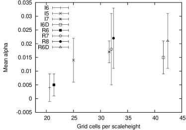
Figure 10: Time-averaged value of the alpha parameter as a function of the number of grid cells in the vertical direction per scale height for all models. The “error bars” correspond to the deviation from the mean value.

In Fig. 10 we plot the values of the alpha parameter as given in Table 1. When increasing the resolution from 32x64x256 (models I6 and R6), to the double resolution of 64x128x512 (models I6D and R6D), the values of the stresses increase considerably. A similar increase of the stresses is observed also when only the resolution in the vertical direction is increased (models I5, I7, R7 and R8), which is analogous to what has been found in the radiative simulations of SKH. A look at Fig. 8 suggests that it is especially the region near the midplane that is not sufficiently resolved, since the stress drops there noticably, while in the better resolved models it does not.

The results depicted in Fig. 10 suggest that once a resolution of about 30 grid cells per scaleheight in the vertical direction has been achieved, the results will no longer significantly depend on the numerical resolution. All models except I6 and R6 are consistent with an $\alpha$-value of about $\alpha\sim 0.015-0.02$, with the isothermal models yielding somewhat lower stresses that are closer to the lower end of $\alpha\sim 0.015$, while the stresses found in the radiative models are grouped around the value $\alpha\sim 0.02$. No tendency is found for the turbulent saturation level to change with respect to neither the vertical box size nor the resolution in the radial and azimuthal directions.

As a consequence of the lower stress, the heating in the low-resolution model R6 is also smaller than compared to the other radiative models, leading to significantly lower temperatures in this model. Apart from this, the temperature profile for model R6 is qualitatively similar to the other models.

As has already remarked before, the heating does intrinsically depend on numerical effects. However, as can be seen from Fig. 5, the temperature profiles for the better resolved models (R7, R8 and R6D) are very similar, suggesting that the heating rates are also converged.

4 Conclusion & Outlook

We have performed 3D radiative MHD simulations of MRI-turbulent protoplanetary discs. Including radiation transport allows us to obtain a self-consistent picture of the vertical structure which results from a dynamic balance between turbulent heating and radiative cooling. Such simulations do thus contain a greater level of realism as compared to previous isothermal simulations. Furthermore, radiative simulations are an important step towards bringing numerical simulations into contact with observations.

In our models two regions can be distinguished: A gas-pressure dominated midplane region where the magnetic field and stresses are approximately constant on average and where almost all the angular momentum transport and dissipation of turbulent energy take place, and a magnetically dominated corona where the stresses and the magnetic field are much smaller than in the midplane region. The position of the photosphere is highly variable due to changing turbulent activity. For most of the time, a large part of the magnetically dominated part of the disc is optically thick. Only at times when the turbulent activity is low do the positions of the photosphere and the magnetosphere coincide.

Since the turbulent saturation level in simulations of MRI turbulence may depend on the numerical resolution, and since in our simulations the heating of the disc is to a large part due to numerical dissipation, it is especially important to check what influence numerical parameters such as the resolution or the box size have on the outcome of the simulation. By running models at different resolutions and with different box sizes, we are able to verify previous results that it is the resolution in the vertical direction that is critical for achieving convergence of the turbulent stresses. We find that once a sufficient resolution in the vertical direction has been achieved ($\sim 30$ grid cells per scaleheight), neither the saturation level nor the heating rates do significantly change when increasing the resolution further. No trend is found for either of these to quantities to change with the vertical box size.

For our model parameters, where we chose to simulate a massive protoplanetary disc, the turbulent heating alone already proved to be sufficient to justify the assumption of ideal MHD. The logical next step will be to include resistivity into the model and choose parameters that are appropriate to a “standard” protoplanetary disc model. When including both non-ideal MHD and radiation transport, it will be possible to do truly self-consistent simulations that do not only include the proper thermodynamics, but also a self-consistently evolved dead zone.

Acknowledgements

This research has been supported in part by the Deutsche Forschungsgemeinschaft DFG through grant DFG Forschergruppe 759 “The Formation of Planets: The Critical First Growth Phase”. Computational resources were provided by the Höchstleistungsrechenzentrum Stuttgart (HLRS) and the High Performance Computing Cluster of the University of Tübingen. We thank Neal Turner for very helpful discussions. We thank an anonymous referee for providing valuable suggestions that helped improve the paper.

Appendix A Implementation of Radiation Transport

In this appendix we describe the implementation of radiation transport into the Cronos MHD code. By adding the thermal energy equation

$$\frac{\partial e_{\mathrm{th}}}{\partial t}+\bm{\nabla}\cdot(e_{\mathrm{th}}\bm{v})=-p\bm{\nabla}\cdot\bm{v}-\kappa_{\mathrm{P}}\rho(4\uppi B-cE_{\mathrm{rad}})$$ (16)

and the radiation energy equation

$$\frac{\partial E_{\mathrm{rad}}}{\partial t}+\bm{\nabla}\cdot(E_{\mathrm{rad}}\bm{v})=-\frac{E_{\mathrm{rad}}}{3}\bm{\nabla}\cdot\bm{v}+\kappa_{\mathrm{P}}\rho(4\uppi B-cE_{\mathrm{rad}})-\bm{\nabla}\cdot\bm{F},$$ (17)

we obtain an equation that describes the evolution of the combined (gas+radiation) energy:

$$\frac{\partial(e_{\mathrm{th}}+E_{\mathrm{rad}})}{\partial t}+\bm{\nabla}\cdot[(e_{\mathrm{th}}+E_{\mathrm{rad}})\bm{v}]=-p_{\mathrm{tot}}\bm{\nabla}\cdot\bm{v}-\bm{\nabla}\cdot\bm{F},$$ (18)

where in general $p_{\mathrm{tot}}=p+E_{\mathrm{rad}}/3$. However, since in our simulations the radiation pressure is small compared to the gas pressure, we neglect it and set $p_{\mathrm{tot}}=p$. Splitting off the radiation diffusion part and making use of the flux-limited diffusion approximation (Levermore & Pomraning, 1981), the radiation transport step becomes:

$$\frac{\partial(e_{\mathrm{th}}+E_{\mathrm{rad}})}{\partial t}=-\bm{\nabla}\cdot\frac{\lambda c}{\kappa\rho}\bm{\nabla}E_{\mathrm{rad}}.$$ (19)

Using the ideal gas law $e_{\mathrm{th}}=c_{\mathrm{V}}\rho T$ and assuming thermal equilibrium between matter and radiation, $E_{\mathrm{rad}}=aT^{4}$, we close our system of equations and end up with the following diffusion equation for the radiation energy:

$$\left(\frac{e_{\mathrm{th}}}{4E_{\mathrm{rad}}}+1\right)\frac{\partial E_{\mathrm{rad}}}{\partial t}=-\bm{\nabla}\cdot\frac{\lambda c}{\kappa\rho}\bm{\nabla}E_{\mathrm{rad}}.$$ (20)

From this we can estimate the timescale to reach thermal balance according to $\tau\sim H^{2}/D_{\mathrm{rad}}$, where $H$ is the scale height and

$$D_{\mathrm{rad}}=\left(\frac{e_{\mathrm{th}}}{4E_{\mathrm{rad}}}+1\right)^{-1}\frac{\lambda c}{\kappa\rho}.$$ (21)

Note that in the radiation pressure dominated case, $D_{\mathrm{rad}}$ is simply given by $D_{\mathrm{rad}}=\lambda c/\kappa\rho$. However, for the gas pressure dominated case that we are considering, we actually have $D_{\mathrm{rad}}=4E_{\mathrm{rad}}\lambda c/e_{\mathrm{th}}\kappa\rho$, which means that $\tau$ is bigger by a factor of $4E_{\mathrm{rad}}/e_{\mathrm{th}}$ and it takes thus much longer to reach thermal balance.

When working in the gas-pressure dominated regime, it is natural to replace the radiation energy $E_{\mathrm{rad}}$ in Eq. (20) by $aT^{4}$ and then solve the following diffusion equation for the temperature:

$$(c_{\mathrm{V}}\rho+4aT^{3})\frac{\partial T}{\partial t}=-\bm{\nabla}\cdot\frac{\lambda c}{\kappa\rho}4aT^{3}\bm{\nabla}T.$$ (22)

This equation is straightforwardly discretised in the following manner:

$$T^{n+1}_{ijk}=T^{n}_{ijk}+\frac{\Delta t}{c_{\mathrm{V}}\rho_{ijk}^{n}+4a(T_{ijk}^{n})^{3}}\Bigg{\{}$$

$$\frac{1}{\Delta x^{2}}\left[D^{n}_{i+\frac{1}{2}jk}\Delta T^{n+1}_{i+\frac{1}{2}jk}-D^{n}_{i-\frac{1}{2}jk}\Delta T^{n+1}_{i-\frac{1}{2}jk}\right]+$$

$$\frac{1}{\Delta y^{2}}\left[D^{n}_{ij+\frac{1}{2}k}\Delta T^{n+1}_{ij+\frac{1}{2}k}-D^{n}_{ij-\frac{1}{2}k}\Delta T^{n+1}_{ij-\frac{1}{2}k}\right]+$$

$$\frac{1}{\Delta z^{2}}\left[D^{n}_{ijk+\frac{1}{2}}\Delta T^{n+1}_{ijk+\frac{1}{2}}-D^{n}_{ijk-\frac{1}{2}}\Delta T^{n+1}_{ijk-\frac{1}{2}}\right]\Bigg{\}},$$

where $\Delta T^{n+1}_{i+\frac{1}{2}jk}=T^{n+1}_{i+1jk}-T^{n+1}_{ijk}$,

$$D^{n}_{i+\frac{1}{2}jk}=\frac{1}{2}\left[\left(\frac{\lambda c}{\kappa\rho}4aT^{3}\right)_{i+1jk}^{n}+\left(\frac{\lambda c}{\kappa\rho}4aT^{3}\right)_{ijk}^{n}\right],$$ (23)

and so on. The resulting matrix equation, which involves a diagonally dominant matrix, can then be solved by any standard matrix solver. For the calculations reported in this paper we used the method of successive overrelaxation.

References

- Balbus (2003) Balbus S. A., 2003, ARA&A, 41, 555
- Balbus (2009) Balbus S. A., 2009, ArXiv e-prints
- Balbus & Hawley (1998) Balbus S. A., Hawley J. F., 1998, Rev. Mod. Phys., 70, 1
- Balsara & Meyer (2010) Balsara D. S., Meyer C., 2010, ArXiv e-prints
- Barge & Sommeria (1995) Barge P., Sommeria J., 1995, A&A, 295, L1
- Bell & Lin (1994) Bell K. R., Lin D. N. C., 1994, ApJ, 427, 987
- Blaes et al. (2006) Blaes O. M., Davis S. W., Hirose S., Krolik J. H., Stone J. M., 2006, ApJ, 645, 1402
- Brandenburg (2008) Brandenburg A., 2008, Physica Scripta, p. 014016
- Carr et al. (2004) Carr J. S., Tokunaga A. T., Najita J., 2004, ApJ, 603, 213
- Chiang & Goldreich (1997) Chiang E. I., Goldreich P., 1997, ApJ, 490, 368
- Davis et al. (2009) Davis S. W., Stone J. M., Pessah M. E., 2009, ArXiv e-prints
- Desch (2007) Desch S. J., 2007, ApJ, 671, 878
- Dzyurkevich et al. (2010) Dzyurkevich N., Flock M., Turner N. J., Klahr H., Henning T., 2010, A&A, 515, A70+
- Flaig et al. (2009) Flaig M., Kissmann R., Kley W., 2009, MNRAS, 394, 1887 (FK2)
- Flock et al. (2010) Flock M., Dzyurkevich N., Klahr H., Mignone A., 2010, A&A, 516, A26+
- Fromang & Nelson (2009) Fromang S., Nelson R. P., 2009, A&A, 496, 597
- Fromang & Papaloizou (2007) Fromang S., Papaloizou J., 2007, A&A, 476, 1113
- Fromang et al. (2007) Fromang S., Papaloizou J., Lesur G., Heinemann T., 2007, A&A, 476, 1123
- Gammie (1996) Gammie C. F., 1996, ApJ, 457, 355
- Hartmann et al. (1998) Hartmann L., Calvet N., Gullbring E., D’Alessio P., 1998, ApJ, 495, 385
- Hawley et al. (1995) Hawley J. F., Gammie C. F., Balbus S. A., 1995, ApJ, 440, 742 (HGB)
- Hayashi (1981) Hayashi C., 1981, Progress of Theoretical Physics Supplement, 70, 35
- Hirose et al. (2006) Hirose S., Krolik J. H., Stone J. M., 2006, ApJ, 640, 901 (HKS)
- Hügelmeyer (2009) Hügelmeyer S., 2009, PhD thesis, Georg-August-Universität Göttingen, Göttingen
- Johansen et al. (2009) Johansen A., Youdin A., Klahr H., 2009, ApJ, 697, 1269
- King et al. (2007) King A. R., Pringle J. E., Livio M., 2007, MNRAS, 376, 1740
- Kissmann et al. (2008) Kissmann R., Kleimann J., Fichtner H., Grauer R., 2008, MNRAS, 391, 1577
- Krolik et al. (2007) Krolik J. H., Hirose S., Blaes O., 2007, ApJ, 664, 1045
- Kurganov et al. (2001) Kurganov A., Noelle S., Petrova G., 2001, SIAM J. Sci. Comput., 23, 707
- Levermore & Pomraning (1981) Levermore C. D., Pomraning G. C., 1981, ApJ, 248, 321
- Miller & Stone (2000) Miller K. A., Stone J. M., 2000, ApJ, 534, 398
- Najita et al. (1996) Najita J., Carr J. S., Glassgold A. E., Shu F. H., Tokunaga A. T., 1996, ApJ, 462, 919
- Pomoell et al. (2008) Pomoell J., Vainio R., Kissmann R., 2008, Sol. Phys., 253, 249
- Pringle (1981) Pringle J. E., 1981, ARA&A, 19, 137
- Sano et al. (2000) Sano T., Miyama S. M., Umebayashi T., Nakano T., 2000, ApJ, 543, 486
- Shakura & Syunyaev (1973) Shakura N. I., Syunyaev R. A., 1973, A&A, 24, 337 (SS)
- Shi et al. (2010) Shi J., Krolik J. H., Hirose S., 2010, ApJ, 708, 1716 (SKH)
- Sicilia-Aguilar et al. (2006) Sicilia-Aguilar A., Hartmann L., Calvet N., Megeath S. T., Muzerolle J., Allen L., D’Alessio P., Merín B., Stauffer J., Young E., Lada C., 2006, ApJ, 638, 897
- Simon et al. (2009) Simon J. B., Hawley J. F., Beckwith K., 2009, ApJ, 690, 974
- Stone et al. (1996) Stone J. M., Hawley J. F., Gammie C. F., Balbus S. A., 1996, ApJ, 463, 656
- Tanga et al. (1996) Tanga P., Babiano A., Dubrulle B., Provenzale A., 1996, Icarus, 121, 158
- Turner (2004) Turner N. J., 2004, ApJ, 605, L45
- Turner & Sano (2008) Turner N. J., Sano T., 2008, ApJ, 679, L131
- Turner et al. (2003) Turner N. J., Stone J. M., Krolik J. H., Sano T., 2003, ApJ, 593, 992