Challenging GRB models through the broadband dataset of GRB 060908

Abstract

Context. Multiwavelength observations of gamma-ray burst prompt and afterglow emission are a key tool to disentangle the various possible emission processes and scenarios proposed to interpret the complex gamma-ray burst phenomenology.

Aims. We collected a large dataset on GRB 060908 in order to carry out a comprehensive analysis of the prompt emission as well as the early and late afterglow.

Methods. Data from Swift-BAT, -XRT and -UVOT together with data from a number of different ground-based optical/NIR and millimeter telescopes allowed us to follow the afterglow evolution from about a minute from the high-energy event down to the host galaxy limit. We discuss the physical parameters required to model these emissions.

Results. The prompt emission of GRB 060908 was characterized by two main periods of activity, spaced by a few seconds of low intensity, with a tight correlation between activity and spectral hardness. Observations of the afterglow began less than one minute after the high-energy event, when it was already in a decaying phase, and it was characterized by a rather flat optical/NIR spectrum which can be interpreted as due to a hard energy-distribution of the emitting electrons. On the other hand, the X-ray spectrum of the afterglow could be fit by a rather soft electron distribution.

Conclusions. GRB 060908 is a good example of a gamma-ray burst with a rich multi-wavelength set of observations. The availability of this dataset, built thanks to the joint efforts of many different teams, allowed us to carry out stringent tests for various interpretative scenarios showing that a satisfactorily modeling of this event is challenging. In the future, similar efforts will enable us to obtain optical/NIR coverage comparable in quality and quantity to the X-ray data for more events, therefore opening new avenues to progress gamma-ray burst research.

1 Introduction

The afterglows of gamma-ray bursts (GRBs) have attracted theoretical and observational interest. The difficulties in building a detailed and consistent model are indeed remarkable. In the context of the “fireball” model, the blastwave is decelerated after sweeping up circumburst medium, and eventually enters a self-similar deceleration regime (Blandford & McKee 1976). The onset of the afterglow, when the fireball begins to decelerate, requires accurate relativistic computations in order to derive reliable (i.e. not only qualitative) predictions (see e.g. Bianco & Ruffini 2005; Kobayashi & Zhang 2007). The scenario emerging from observations both in the X-rays and at longer wavelengths (optical, near-infrared; hereafter NIR) appears to be even more complicated than expected only a few years ago, with the superposition of emission from different mechanisms beyond the external shock emission.

Swift-XRT observations have provided an increasing sample of well-monitored observations, allowing for the derivation of the well-known “canonical” X-ray light-curve (Nousek et al. 2006). As shown by many authors (e.g. Panaitescu 2006; Zhang et al. 2007b; Panaitescu 2007; Takami et al. 2007; Willingale et al. 2010), the early X-ray afterglow is often dominated by a steeply decaying emission component usually attributed to large-angle emission produced during the main burst (Fenimore et al. 1996; Tagliaferri et al. 2005; Zhang et al. 2006; Liang et al. 2007), although it has also been attributed to progressively fading central engine activity (Fan & Wei 2005; Fan et al. 2008; Kumar et al. 2008). The subsequent “shallow-decay” phase (for an overview, see Liang et al. 2007) is still attributed to prolonged central engine activity (Fan & Piran 2006; Jóhannesson et al. 2006), although there are other proposed mechanisms which can be at work: ejecta with a wide Lorentz $\Gamma$-factor energy distribution (Rees & Mészáros 1998), varying micro-physics parameters (Panaitescu 2007), delayed burst emission due to dust-scattering (e.g. Shao & Dai 2007; Shen et al. 2009, who reach different conclusions), off-axis initial observation (Granot 2005; Donaghy 2006; Guidorzi et al. 2009), etc.

In the optical/NIR the situation is somewhat less defined. Robotic telescopes throughout the world have provided early-time light curves often fully overlapped in time to the Swift-XRT (and -UVOT) observations. The data quality, however, is not always adequate for a detailed modelling, due to the modest aperture of most robotic, rapid-pointing, telescopes. For several events it was possible to detect the afterglow (external shock) onset (Vestrand et al. 2006; Molinari et al. 2007; Ferrero et al. 2009; Rykoff et al. 2009; Klotz et al. 2009) as predicted by semi-analytical estimates (Sari & Piran 1999) and more accurate numerical analyses (Kobayashi & Zhang 2007; Jin & Fan 2007). The lack of reverse shock (see e.g. Mundell et al. 2007; Jin & Fan 2007) confirms the general results for Swift GRBs obtained by the UVOT (Roming et al. 2006). These (lack of) findings impose severe constraints on the micro-physics parameters of the relativistic shocks or alternatively suggests that additional ingredients, such as magnetically dominated outflows, are required (Lyutikov et al. 2003; Fan et al. 2004; Zhang & Kobayashi 2005). The prompt emission from GRB 990123 (Akerlof et al. 1999), considered to be a typical example of reverse shock emission peaking in the optical, was also interpreted as the long wavelength tail of the large-angle high-energy emission from the prompt event (Panaitescu & Kumar 2007). Reverse shock emission was invoked to model the early-time post-flash optical emission of the exceptionally bright GRB 080319B (Bloom et al. 2009; Kumar & Panaitescu 2008; Racusin et al. 2008; Yu et al. 2009). A comparable emission due to the reverse and forward shock was also proposed for GRB 070802 (Krühler et al. 2008). Partly motivated by the increasing difficulties of the so-called “standard model” in interpreting the rich multi-wavelength datasets now available, there is a rising interest in alternative scenarios, such as the “cannonball” model (Dado & Dar 2009; Dado et al. 2009). This scenario has shown remarkable fitting capabilities (e.g. Dado & Dar 2010a, b) although it is still lacking of a comprehensive independent analysis campaign.

Some classification schemes have been proposed to interpret the rich variety displayed by optical afterglows. Zhang et al. (2003) and Jin & Fan (2007) define three classes, depending on the mutual importance of the reverse and forward shock emission based on theoretical considerations. Class I is constituted by afterglows showing both the reverse and forward shock emissions, class II is for afterglows with a prominent reverse shock emission outshining all other components, and class III contains events characterised by forward shock emission only. Panaitescu & Vestrand (2008) observationally classify the optical afterglows in four classes following the temporal behaviour of the early optical emission and try to find a common scenario producing all the different observed behaviours: fast-rising with an early peak, slow-rising with a late peak, flat plateau, and rapid decays since the first measurements. They conclude that an emission due to the forward or reverse shock coming from a structured collimated outflow can explain all the four shapes, by varying the observer location and the structure of the outflows. However, the afterglows with plateaus and slow rises could also be due to a long-lived injection of energy in the blast wave. Interestingly, these authors find a possible peak flux-peak time correlation for the fast- (extended to slow-) rising optical afterglows that could provide a way to use them as standard candles. Note however that Klotz et al. (2009) and Kann et al. (2009) with more data later questioned the tightness of the correlation. Liang et al. (2009) discovered a set of correlations between afterglow onset parameters in the optical and GRB parameters, in particular a tight correlation between the initial Lorentz factor and the burst isotropic energy (see also Dado & Dar 2010b). Moreover, as clearly demonstrated by the case of GRB 050820A (Vestrand et al. 2006) or GRB 080319B (Racusin et al. 2008), the possible influence of the optical emission coming from the prompt GRB phase should also be taken into account when analysing the early light curve, further complicating the picture.

In general, a satisfactory understanding of the early afterglow phases is still lacking. Events with high-quality optical early-time observations carried out with robotic telescopes and/or the UVOT are thus especially important for testing the predictions of different models. We discuss here the case of GRB 060908. In Sect. 2 we report the main observational data available for this event. In Sect. 3 we give some details of the data analysis for Swift-BAT, -XRT, -UVOT, REM, SMARTS, Danish 1.54m, NOT, UKIRT, TNG and the Plateau de Bure Interferometer observations and in Sect. 4 we discuss our results. Our main conclusions are given in Sect. 5.

2 GRB 060908

GRB 060908 was detected by the Swift satellite (Gehrels et al. 2004) on Sept. 8, 2006 at 08:57:22 UT (Evans et al. 2006). Further analysis (see Sect. 3.1) yielded a revision of the GRB time. The optical afterglow was detected from ground by the PROMPT telescope showing a bright ($r\sim 15$ mag about 105 s after the burst), rapidly fading source (Nysewander et al. 2006). The optical afterglow was then confirmed at coordinates RA=02:07:18.3 and DEC=+00:20:31 (J2000, 0.5″ error) with the REM telescope by Antonelli et al. (2006) reporting $R\sim 17$ mag about 7 min after the burst. A first estimate of the decay rate was provided by Wiersema et al. (2006) as $\alpha=1.07\pm 0.11$, with observations carried out with the Danish 1.54m telescope at ESO-La Silla equipped with DFOSC. Later observations were also reported by Andreev et al. (2006).

Rol et al. (2006) derived a redshift identifying the absorption lines of C IV and Si II, and possibly Al III by means of observations performed with the Gemini-North telescope equipped with GMOS. Their redshift estimate was later corrected by Fynbo et al. (2009) to $z=1.884\pm 0.003$. The afterglow was not detected at 8.46 GHz with the VLA a day after the burst with a $3\sigma$ upper limit of 77 $\mu$Jy (Chandra & Frail 2006). The effect of the host galaxy on the light-curve was initially detected by Thöne et al. (2006) with the NOT equipped with ALFOSC.

Throughout the paper, the decay and energy spectral indices $\alpha$ and $\beta$ are defined by $F_{\nu}(t,\nu)\propto(t-T_{0})^{-\alpha}\nu^{-\beta}$, where $T_{0}$ is the onset time of the burst. We assume a $\Lambda{\rm CDM}$ cosmology with $\Omega_{\rm m}=0.27$, $\Omega_{\Lambda}=0.73$ and $h_{0}=0.71$. At the redshift of the GRB ($z=1.88$), the luminosity distance is $\sim 15$ Gpc ($\sim 4.5\times 10^{28}$ cm, corresponding to a distance modulus $\mu=45.8$ mag). The Galactic extinction in the direction of the afterglow is E${}_{B-V}=0.03$ mag (Schlegel et al. 1998). All errors are $1\sigma$ unless stated otherwise.

3 Observations, data reduction and analysis

3.1 Swift-BAT

GRB 060908 triggered BAT at 08:57:22.34 UT, which hereafter will be referred to as $T_{\rm BAT}$. We extracted the mask-weighted light curves and energy spectra in the 15–150 keV band following the BAT team instructions. The 15–150 keV prompt emission profile consists of an initial structure where three pulses can be identified lasting about 15 s, followed by a 5 s long quiescent time ended by another isolated pulse comparable with the previous ones (Fig. 1). The total duration (15–150 keV) in terms of $T_{90}$ is $19.3\pm 0.3$ s (Palmer et al. 2006). We note that the onset of the GRB, $T_{0}$, occurs before the trigger time $T_{\rm BAT}$: in particular, we find $T_{0}=T_{\rm BAT}-12.96$ s from significance requirements described below. This was also pointed out by the BAT team (Palmer et al. 2006). Also worth mentioning is the evidence of a weak prolonged emission at high energies, when the light curves were binned to reach a given significance in the count rate of each bin. Fig. 2 shows the case of the 15–150 keV profile when 3$\sigma$ are required for each time bin. The last point from $T_{0}+26.1$ s to $T_{0}+975.2$ s is 2.7$\sigma$ significant. Notably, this is broadly concurrent with some flaring activity in the soft X-rays detected by the Swift/XRT (see Sect. 3.2).

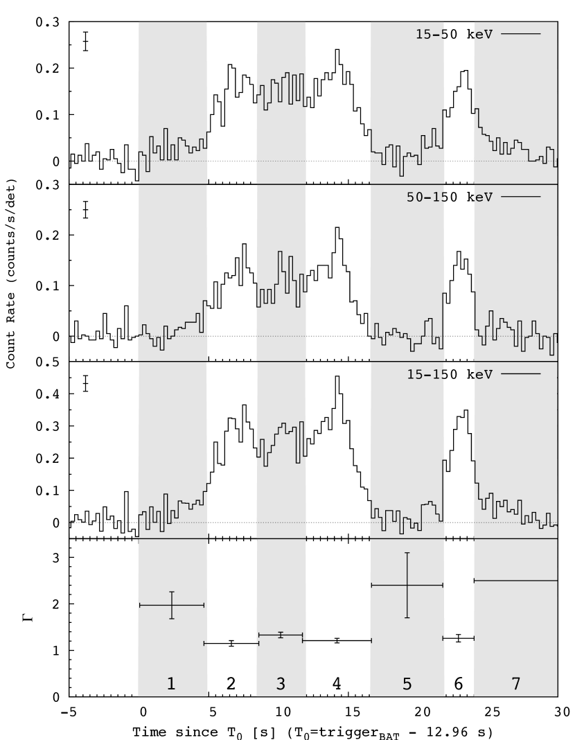
Figure 1: BAT mask-weighted light curves of the prompt emission in the 15–50, 50–150 and 15–150 keV energy bands from the top downward, respectively. Times refer to the revised BAT trigger time ($T_{0}=T_{\rm BAT}-12.96$ s) The vertical bar shown at the top left corner in each plot shows the typical error on the count rate. The time binning is 0.256 s. The count rates are expressed in units of counts s^-1 per fully illuminated detector for an equivalent on-axis source. The bottom panel shows the spectral photon index as a function of time.

Energy spectra were extracted in seven contiguous time intervals as reported in Fig. 1. The choice was driven by the light curve evolution: we identified the first rise (1), the three overlapping pulses of the first structure (2–4), the quiescent time (5), the following isolated pulse (6) and the final long weak tail (7). All of the spectra can be fit with a single power law. Detailed results of the spectral fitting are reported in Table 1.

Table 1: BAT energy spectra (15–150 keV) in the seven distinct time intervals of the prompt emission. Each interval is fit with a power law ($\Gamma$ is the photon index). Times are referred to the revised BAT trigger time ($T_{0}=T_{\rm BAT}-12.96$ s). Uncertainties are 1$\sigma$.

#	$T_{\rm start}$	$T_{\rm stop}$	$\Gamma$	Fluence	$\chi^{2}$/dof
	(s)	(s)		($10^{-7}$ erg cm-2)
1	$0.00$	$4.66$	$1.97\pm 0.29$	$1.0\pm 0.2$	$11.63/7$
2	$4.66$	$8.59$	$1.15\pm 0.06$	$6.8\pm 0.25$	$47.44/47$
3	$8.59$	$11.71$	$1.33\pm 0.06$	$5.5\pm 0.22$	$41.20/41$
4	$11.71$	$16.66$	$1.21\pm 0.05$	$9.0\pm 0.3$	$35.80/47$
5	$16.66$	$21.76$	$2.4\pm 0.7$	$0.54\pm 0.19$	$0.05/1$
6	$21.76$	$24.00$	$1.26\pm 0.08$	$3.8\pm 0.2$	$46.43/43$
7	$24.00$	$975.3$	$2.5\pm 1.0$	$2.8\pm 1.5$	$3.33/4$
total	$0.0$	$28.0$	$1.36\pm 0.04$	$27.6\pm 0.6$	$46.8/46$

Figures 1 and 2 display the 15–150 keV light curve and the evolution of the spectral photon index. We can see a hardening around the peaks of the pulses similar to the canonical behaviour of other GRBs. Apart from this, the prompt emission does not exhibit strong spectral evolution, the photon index being pretty constant along different pulses and consistent with that derived from the total spectrum, $\Gamma_{\rm tot}=1.36\pm 0.04$. The total fluence in the 15–150 keV band is $(2.8\pm 0.1)\times 10^{-6}$ erg cm^-2, $\sim$10% of which from the weak long tail after $T_{0}+24.00$ s. These results are also in agreement with those by Palmer et al. (2006).

Figure 2: Top panel: 15–150 keV mask-weighted light curve of the prompt emission up to 1000 s after the trigger time. The binning is variable and was determined so as to have at least 3$\sigma$ significant rates in each bin, except for the last point from $T_{0}+26.1$ s to $T_{0}+975.2$ s which is at 2.7$\sigma$ ($T_{0}=T_{\rm BAT}-12.96$ s). Dashed lines show the last point split into three bins: in particular we note detection of emission from $T_{0}+453$ s to $T_{0}+529$ s the 2.2$\sigma$. Bottom panel: temporal evolution of the spectral photon index $\Gamma$.

Unfortunately, no measurement of the peak energy $E_{\rm p}$ of the time-integrated spectrum is available. However, from the hardness of $\Gamma_{\rm tot}$ we can infer that $E_{\rm p}$ lies above the BAT passband or close to its upper bound. Indeed, if we fit the total spectrum with a Band function (Band et al. 1993) and fix the high energy photon index $\beta$ at the typical value $\beta=-2.3$, we find for the low-energy index $\alpha=-0.9\pm 0.3$ and $E_{\rm p}=133_{-33}^{+120}$ keV with $\chi^{2}/{\rm dof}=38.5/45$ (90% errors), in fair agreement with the estimate by Ghirlanda et al. (2008) and Sakamoto et al. (2009). This is also consistent with the empirical relation between $E_{\rm p}$ and $\Gamma$ (measured by BAT) for a number of bursts (Zhang et al. 2007a). Assuming this value for $E_{\rm p}$, we derive the following values: $E_{\rm p,i}=383_{-95}^{+346}$ keV (rest-frame peak energy) and $E_{\rm iso}=(6.2\pm 0.7)\times 10^{52}$ erg (isotropic-equivalent released energy in the rest-frame $1-10^{4}$ keV energy band, errors at 90%).

3.2 Swift-XRT

The XRT observations of GRB 060908 started at 08:58:42 UT, about $\sim 80$ s after the BAT trigger, and ended on September 20, 2006 at 23:01:56 UT. The XRT afterglow candidate alert was delivered about 100 s after the BAT trigger. The monitoring consisted of 14 different observations. The first data were taken in windowed timing (WT) mode and lasted for $\sim 100$ s. After that, the on-board measured count rate was low enough for the XRT to switch to the photon counting (PC) mode; for the rest of the follow-up, XRT remained in PC mode.

The XRT data were reduced using the xrtpipeline task (v.2.5), applying standard calibration and filtering criteria, i.e., we cut out temporal intervals in which the CCD temperature was above $-47\,^{\circ}$C and we remove hot and flickering pixels. An on-board event threshold of $\sim 0.2$ keV was applied to the central pixel; this was proven to reduce most of the background due to the bright Earth and/or the CCD dark current. We selected XRT grades 0-2 and 0-12 for WT and PC data, respectively.

The intensity of the source was high enough to cause significant pile-up in the first part of the PC mode observations. In order to correct for the pile-up, we extracted the counts from an annulus with an inner radius of 4 pixels and an outer radius of 20 pixels (9″ and 47″, respectively). We then corrected the observed count rate for the fraction of the XRT point spread function (PSF) lying outside the extraction region. Data in WT mode were not affected by pileup; thus, for WT observations and for the remaining PC observations, a region of 20 pixel radius was selected. Physical ancillary response files were generated using the task xrtmkarf, to account for different extraction regions.

Table 2: Spectral analysis of the Swift-XRT data. The switch from WT to PC mode occurred at $\sim 180$ s after the burst. Analysis of data later than about 2000 s gave results comparable to those for the PC mode but with lower statistical significance.

Mode	NH	NH	Photon index	$\chi^{2}$/dof
		(rest frame)
	($10^{21}$cm-2)	($10^{21}$cm-2)
WT	$7.2_{-4.6}^{+5.2}$	-	$2.32_{-0.29}^{+0.33}$	17.9/17 = 1.05
PC	$14.1_{-6.0}^{+7.0}$	-	$2.32_{-0.20}^{+0.20}$	11.9/17 = 0.70
WT	$0.23$	$3.6_{-3.0}^{+3.6}$	$2.28_{-0.17}^{+0.20}$	17.7/17 = 1.03
PC	$0.23$	$8.3_{-3.7}^{+5.7}$	$2.17_{-0.22}^{+0.25}$	12.9/17 = 0.76

For spectral analysis we used redistribution matrices version 11. Spectral fit results are reported in Table 2. The spectra were modeled with a simple absorbed power-law. The Galactic column density around the GRB 060908 position is $2.3\times 10^{20}$ cm^-2 (Kalberla et al. 2005). By fitting a power law model with a Galactic contribution fixed at the above value, we derive an intrinsic column density of $8.3^{+5.7}_{-3.7}\times 10^{21}$ cm^-2 for data collected in PC mode, where spectral variability is lower. This is in line with rest-frame absorption observed in GRBs (Campana et al. 2010).

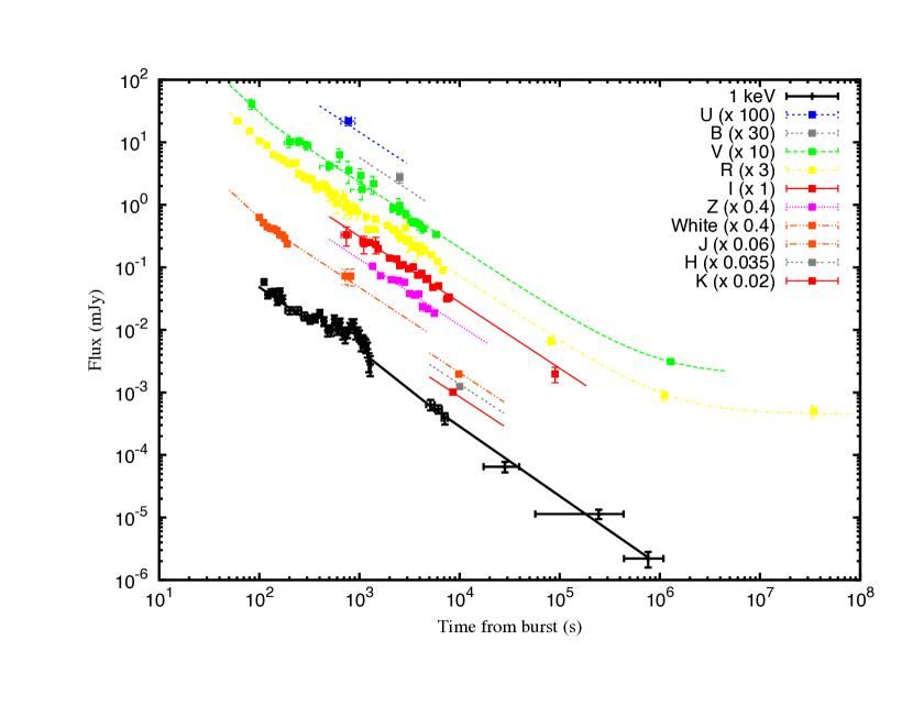
Figure 3: Light curve in the X-ray and optical/NIR bands for the afterglow of GRB 060908. The light curves are fitted with a simple power-law with index $\sim 1.1$ for the X-ray data while two power-laws smoothly joined are applied to optical/NIR data. The time delay from the burst was corrected as $T_{0}=T_{\rm BAT}-12.96$ s (see Sect. 3.1).

The total light curve in physical units is shown in Fig. 3. The curve is characterised by a constant power-law decay with index $\alpha\sim 1.1$, while from about 200 to 1000 s a complex, although not strongly dominant, flaring activity is superposed on the continuous decay. Apart from these flares, the decay goes on uninterrupted up to the last XRT observations at $\sim 10^{6}$ s from the burst. We could model ($\chi^{2}/{\rm dof}=35.6/33=1.08$) the XRT light curve with a simple power-law with decay index $\alpha_{\rm X}=1.12_{-0.02}^{+0.05}$, plus two Gaussians (Fig. 4 to fit the main flares. Since we are mainly interested in the behaviour of the underlying afterglow, the Gaussian function representing the flares was chosen for simplicity, and no physical meaning is attributed to them. A more detailed analysis of flaring activity in this and other events is reported in Chincarini et al. (2010). Liang et al. (2008) claimed a possible identification of a break in the Swift-XRT light-curve. GRB 060908 was indeed classified as part of their “bronze” class, i.e. events showing a break with post-break decay index steeper than 1.5. This is due to the neglecting of the effect of the end of the flaring activity at about 1000 s.

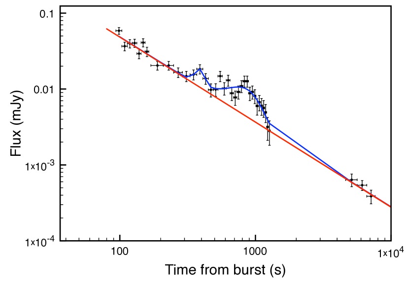
Figure 4: Light curve at 1 keV for the Swift-XRT observation around the epoch of the small flares superposed on the afterglow power-law decay. The blue solid line is a fit with a temporal power-law decay with index $\sim 1.1$ and two Gaussians centred at $\sim 390$ and $\sim 810$ s from the burst. The red line shows the power-law only component. The time delay from the burst was corrected as $T_{0}=T_{\rm BAT}-12.96$ s (see Sect. 3.1).

3.3 Optical/NIR data

Swift-UVOT (Roming et al. 2005) data were retrieved from the HEASARC public archive. UVOT data analysis was carried out following standard recipes. The data were screened for standard bad times, South Atlantic Anomaly passages, Earth limb avoidance, etc. The task uvotsource was applied to compute aperture photometry for images, and uvotevtlc for event files. Photometry in the $UBV$ broad band filters and without filter (“white”) was derived with radii of 6 ″  and 12 ″  of aperture for image and event file analysis, respectively. For the bluer filters UVW1, UVM2 and UVW2, a radius twice as large was used. We also verified the consistency between image and event file photometry for a set of bright, isolated, unsaturated stars. Consistency between UVOT and REM photometry for the $V$ band was also checked. The UVOT alert was delivered about 15 min after the BAT trigger but UVOT observations had already started about one minute after the trigger. The results are reported in Table 3.

Table 3: Light-curve data of the GRB 060908 afterglow obtained by our collaboration. The time delay from the burst was updated as $T_{0}=T_{\rm BAT}-12.96$ s (see Sect. 3.1). Galactic extinction has not been removed from these data.

Band	$T-T_{0}$	Bin half size	Magnitude	Telescope
	(s)	(s)
$U$	778	125	$17.05\pm 0.18$	UVOT
$B$	2522	22.5	$19.10\pm 0.20$	SMARTS
$V$	84	2.5	$14.87\pm 0.20$	UVOT
	202	25	$16.38\pm 0.21$	UVOT
	252	25	$16.37\pm 0.15$	UVOT
	302	25	$16.52\pm 0.17$	UVOT
	500	100	$17.34\pm 0.17$	UVOT
	633	10	$16.88\pm 0.26$	REM
	783	10	$17.50\pm 0.42$	REM
	1034	30	$17.71\pm 0.29$	REM
	1063	250	$18.28\pm 0.35$	UVOT
	1385	30	$18.04\pm 0.35$	REM
	2522	15	$18.90\pm 0.30$	SMARTS
	1278472	2100	$25.04\pm 0.10$	NOT
$R$	61	5	$14.02\pm 0.04$	REM
	80	5	$14.43\pm 0.06$	REM
	100	5	$14.83\pm 0.06$	REM
	119	5	$15.00\pm 0.08$	REM
	138	5	$15.38\pm 0.10$	REM
	157	5	$15.48\pm 0.12$	REM
	176	5	$15.60\pm 0.12$	REM
	195	5	$15.73\pm 0.12$	REM
	214	5	$15.74\pm 0.13$	REM
	233	5	$15.71\pm 0.14$	REM
	248	10	$16.14\pm 0.14$	REM
	277	10	$16.25\pm 0.15$	REM
	306	10	$16.32\pm 0.16$	REM
	336	10	$16.35\pm 0.16$	REM
	365	10	$16.63\pm 0.21$	REM
	394	10	$16.67\pm 0.20$	REM
	423	10	$16.63\pm 0.18$	REM
	452	10	$16.58\pm 0.20$	REM
	481	10	$16.73\pm 0.21$	REM
	510	10	$16.93\pm 0.26$	REM
	542	10	$17.11\pm 0.25$	REM
	571	10	$16.95\pm 0.23$	REM
	601	10	$17.34\pm 0.34$	REM
	695	10	$17.08\pm 0.28$	REM
	724	10	$17.48\pm 0.36$	REM
	753	10	$17.36\pm 0.33$	REM
	825	30	$17.65\pm 0.27$	REM
	894	30	$17.49\pm 0.24$	REM
	964	30	$17.64\pm 0.27$	REM
	1211	65	$18.36\pm 0.36$	REM
	1420	136	$18.37\pm 0.34$	REM
	2177	30	$18.36\pm 0.07$	Danish
	2461	30	$18.56\pm 0.06$	Danish
	2522	15	$18.70\pm 0.10$	SMARTS
	2652	60	$18.72\pm 0.06$	Danish
	2864	25	$18.29\pm 0.40$	REM
	2874	60	$18.79\pm 0.06$	Danish
	3100	201	$18.77\pm 0.40$	REM
	3125	90	$18.86\pm 0.06$	Danish
	3402	90	$19.00\pm 0.06$	Danish
	3683	90	$19.06\pm 0.06$	Danish
	3787	334	$19.03\pm 0.43$	REM
	4018	120	$19.02\pm 0.05$	Danish
	82747	7317	$22.83\pm 0.16$	Danish
	1113287	2400	$25.00\pm 0.20$	NOT
	34343882	2865	$25.63\pm 0.25$	TNG
$I$	740	85	$17.17\pm 0.37$	REM
	1105	30	$17.52\pm 0.34$	REM
	1456	30	$17.55\pm 0.32$	REM
	2522	22.5	$18.40\pm 0.10$	SMARTS
$J$	9819	405	$19.22\pm 0.06$	UKIRT
$H$	10039	405	$18.65\pm 0.08$	UKIRT
$K$	8586	520	$17.80\pm 0.03$	UKIRT
White	100	5	$15.23\pm 0.11$	UVOT
	110	5	$15.44\pm 0.10$	UVOT
	120	5	$15.60\pm 0.10$	UVOT
	130	5	$15.67\pm 0.10$	UVOT
	140	5	$15.69\pm 0.10$	UVOT
	150	5	$15.76\pm 0.10$	UVOT
	160	5	$15.92\pm 0.11$	UVOT
	170	5	$15.94\pm 0.10$	UVOT
	180	5	$16.06\pm 0.11$	UVOT
	190	5	$16.28\pm 0.12$	UVOT
	720	25	$17.57\pm 0.30$	UVOT
	820	25	$17.58\pm 0.33$	UVOT

REM is a 60 cm diameter fast-reacting (10^∘ s^-1 pointing speed) telescope located at the Cerro La Silla premises of the European Southern Observatory (ESO), Chile (Zerbi et al. 2001; Chincarini et al. 2003; Covino et al. 2004a, b). The telescope hosts REMIR, an infrared imaging camera, and ROSS, an optical imager and slitless spectrograph. The two cameras observe simultaneously the same field of view of $10$′$\times 10$′ thanks to a dichroic. Unfortunately, REMIR could not observe this GRB due to maintenance work. The Swift-BAT alert was received by the REM telescope 14.7 s after the BAT trigger time. The telescope reacted automatically and was tracking the GRB field 34.1 s after receipt of the alert (48.8 s after the BAT trigger). ROSS data ($V,R$ and $I$ bands) and other ground based telescope data were reduced in a standard way by means of tools provided by the ESO-Eclipse package (Devillard 1997). Photometry for REM data and other ground based telescopes was carried out with SExtractor (v. 2.5.0; Bertin & Arnouts 1995). Photometric calibration was accomplished by using instrumental zero points, checked with observations of standard stars in the SA 110 Landolt field (Landolt 1992). The results are reported in Table 3.

We also obtained data for two nights using the Danish 1.54 m telescope at ESO - La Silla, Chile. We used the Danish Faint Object Spectrograph and Camera (DFOSC) instrument, which has a 13′.7 $\times$ 13′.7  field of view, with a pixel scale of 0$\aas@@fstack{\prime\prime}$395 per pixel. Our observations on the first night consisted of a series of short exposures in the $R$ band (and one in the $I$ band), increasing in exposure time to obtain comparable photometric uncertainties in each datapoint. The data taken on the second night consist of a series of $R$ band images with exposure ranging from 5 to 10 min. Multicolour observations within 1 hr after the burst were also obtained with the SMARTS 1.3 m telescope. Calibration was carried out by means of secondary standard stars derived from the calibration of the REM data.

NIR observations about 10 ks after the GRB have been provided by the UKIRT 3.8m telescope at Mauna Kea, Hawaii Islands, USA. We used the WFCAM wide field camera ($0\degr.75\times 0\degr.75$). The data were reduced and analysed following standard NIR recipes. We carried out late time observations with the Nordic Optical 2.5m Telescope equipped with the ALFOSC and the TNG equipped with DOLoRes. Both telescopes are located at the Canarian island of La Palma. These observations were aimed at detecting the host galaxy of GRB 060908. NOT observations were carried out under variable meteorological conditions on 2006 Sept. 21 ($R$ band) and 23 ($V$ band), about 12-14 days after the GRB). TNG observations were carried out under good observing conditions on 2007 Oct. 10, more than one year after the burst. An object compatible with the afterglow position was visible. In consideration of the long delay this might well be the host galaxy ($R\sim 25.6$, Table 3). Reduction was performed in a standard way and calibration was carried out by using secondary standards in the field. Finally, we used published optical data obtained with the Palomar 60 inch telescope from Cenko et al. (2009).

The total light curve is shown in Fig. 3 (see also Table 3). Optical data were fitted by using power-law models for both the light-curve and spectra. The light-curve appears characterised by an initial steeper decay (see also Oates et al. 2009; Kann et al. 2009) with $\alpha_{\rm optNIR}\sim 1.4$ followed by a flattening, $\alpha_{\rm optNIR}\sim 1$ with a transition time of about 120-360 s. At later times the optical light curve began to be dominated by the host galaxy. Any late-time break is therefore difficult to locate. There was no clear spectral evolution. A single rather blue power-law, $\beta_{\rm optNIR}\sim 0.3$, provided a satisfactory description (Fig. 5) with some local, unconstrained, rest-frame absorption, E${}_{B-V}\sim 0.03$, following the Small Magellanic Cloud (SMC) extinction curve (Pei 1992). Extinction curves typical of the Large Magellanic Cloud, the Milky Way (Pei 1992) or starburst galaxies (Calzetti et al. 2000) environments gave worse fits. Forcing a late break improves the global fit significantly, though the break time is not well constrained. Considering that the number of different telescopes, filters, observing conditions, etc. might have introduced some inhomogeneity in the data, and artificially pushed the resulting $\chi^{2}$ up, we consider both possibilities (two or three power-laws in time) in the later discussion. Best-fit parameters and corresponding errors are reported in Table 4.

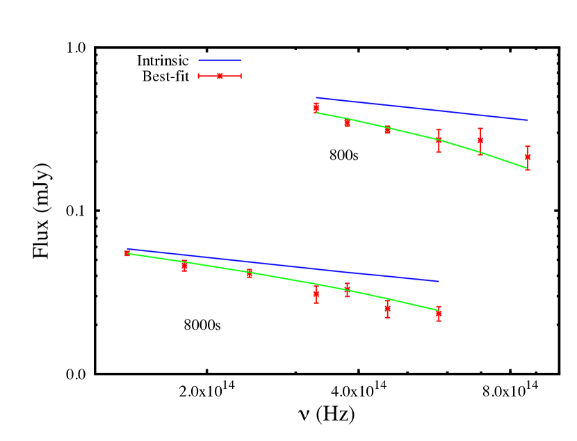
Figure 5: Optical/NIR SEDs obtained at 800 and 8000s. The best-fit model including Milky-Way and rest-frame absorption and the intrinsic spectral shape are reported.

Table 4: Optical/NIR light curve best fit results for models consisting of two (2PL) or three power laws (3PL). Spectral data are always fit with a single power-law plus possible rest-frame absorption following the SMC extinction curve and the known Galactic absorption. Upper limits are at 95% confidence level.

	2PL	3PL
$\alpha_{1}$	$1.48_{-0.25}^{+0.24}$	$1.32_{-0.13}^{+0.19}$
$t_{{\rm b}_{1}}$ (s)	$138_{-43}^{+167}$	$365_{-228}^{+411}$
$\alpha_{2}$	$1.05_{-0.03}^{+0.03}$	$0.94_{-0.36}^{+0.10}$
$t_{{\rm b}_{2}}$ (s)	-	$2360_{-900}^{+4300}$
$\alpha_{3}$	-	$1.15_{-0.06}^{+0.24}$
$\beta$	$0.17_{-0.40}^{+0.34}$	$0.33_{-0.29}^{+0.25}$
EB-V (mag)	$<0.10$	$<0.10$
$\chi^{2}/{\rm dof}$	$159.1/121=1.32$	$133.8/119=1.12$

3.4 Millimetre observations

We complete our dataset with limits at millimetre wavelengths obtained with the Plateau de Bure Interferometer (Guilloteau et al. 1992). We observed the field at a mean time of 02:02 UT on 2009 Sept. 9 (17 hr after the burst onset) simultaneously at 92 GHz (3 mm) and 236 GHz (1 mm) using the 5Dq compact five antenna configuration. Data calibration was done using the GILDAS software package using MWC349 as flux calibrator, 3C454.3 as bandpass calibrator and 0235+164 as amplitude and phase calibrator. We did not detect any source at the position of the GRB afterglow with 3$\sigma$ limit of 1.17 mJy in the 92 GHz band and 9.9 mJy in the 236 GHz band. This is consistent with the limit reported by Chandra & Frail (2006) (see Sect. 2).

4 Discussion

4.1 Prompt emission

The prompt emission of GRB 060908 lasted $19.3\pm 0.3$ s (Palmer et al. 2006). The corresponding spectra (Table 1) were typical of the long-soft class of GRBs (Kouveliotou et al. 1993), although the average photon index for the GRB 060908 prompt emission is rather close to the hard tail for the long/soft GRB distribution (Sakamoto et al. 2008). Spectral lag was also originally proposed by Norris et al. (2000) and Norris & Bonnell (2006) as a possible tool to better discriminate between GRB classes. Recently, Ukwatta et al. (2009), in a comprehensive study of spectral lags for a sample of 31 GRBs with measured redshift, reported for GRB 060908 a spectral lag consistent with zero. However, the errors were large enough to prevent firm conclusions. With the estimated isotropic and peak energies, GRB 060908 would lie within 2$\sigma$ of the “Amati” relation (Amati et al. 2002; Amati 2006). Applying the $E_{\rm iso}-\Gamma_{0}$ relation singled out by Liang et al. (2009) the initial Lorentz factor should be $\Gamma_{0}\sim 300$ (see Sect. 4.2).

No precursor was seen in the Swift-BAT light-curve and the high energy emission did not show any detectable spectral evolution. The light-curve showed two periods of activity separated by a pause lasting a few seconds. The spectra during activity periods were substantially harder than that in the relatively quiescent interval; this is in agreement with previous findings about a general intensity-hardness correlation during prompt emission (Golenetskii et al. 1983; Borgonovo et al. 2001), which has been attributed to the curvature effect by Qin (2009). After the prompt emission a longer-lasting soft emission is detectable, possibly up to about 1000 s.

4.2 The early afterglow

The pulse at about 23 s after the beginning of the prompt emission might mark the onset of the afterglow, which can usually be hidden by longer prompt activity. In this case the duration of the observed prompt emission would be just $\sim 15$ s. Following this hypothesis, it is possible to estimate the initial Lorentz bulk motion $\Gamma_{0}$ by using the method describeed in Molinari et al. (2007). The dependence of $\Gamma_{0}$ on environment parameters is weak and we can assume a constant density circumburst medium due to the rapid increase in flux before the onset. Under these assumptions in the so-called “thin-shell” case, and applying Eq. 1 in Molinari et al. (2007) where $\Gamma_{0}=2\Gamma$, the initial Lorentz factor turns out to be $\Gamma_{0}\sim 700\,(\eta_{0.2}n_{0})^{-1/8}$, where $\eta$ in units of $0.2$ is the radiative efficiency and $n_{0}$ the circumburst constant number density in cm^-3. This figure is in agreement with theoretical expectations (Zhang & Meśzáros 2004) and close to recent estimates for a few GRBs in which prompt GeV photon emission was detection with the Fermi satellite (e.g. Abdo et al. 2009; De Pasquale et al. 2010; Ghirlanda et al. 2010). This hypothesis, though intriguing, has also substantial difficulties. The last pulse of the prompt emission shows a time profile comparable to that of the other prompt emission pulses, suggesting a common origin. Moreover, it is characterized by a rather hard photon index, $\Gamma=1.26\pm 0.08$, comparable, as noted above, to the spectral parameters of the periods of high activity of the prompt emission. While similar to the optical/NIR spectral index, it is much harder than the initial X-ray afterglow spectral index (and of the long-lasting BAT emission detected at the end of the prompt phase). Such a complex spectral shape strongly suggests that the last pulse is part of the prompt emission, and is not related to the forward shock. In order to interpret the last pulse of the prompt emission as the afterglow onset we at least need to assume that the spectrum of the X-ray and optical/NIR afterglow observed about a minute after the high-energy event has already spectrally evolved remarkably soon after the onset.

Following the Panaitescu & Vestrand (2008) classification, GRB 060908 is a clear example of afterglow that is decaying since the first observation. The authors suggest that, in a scenario of a structured outflow observed from different locations, this class of optical light curves could correspond to an observer location within the aperture of the brighter outflow core, with higher Lorentz factor and, therefore, a shorter deceleration time-scale. We can check whether GRB 060908 is consistent with the peak flux - peak time correlation found for initially rising afterglows. Our first observation is at $t\sim 61$ s. The corresponding flux emission at 2 eV predicted by Eq. 2 of Panaitescu & Vestrand (2008, scaled to the redshift of GRB 060908), assuming we detected the peak optical flux, is $f_{\rm p}\sim 560$ mJy ($R\sim 9.4$). The dereddened 2 eV observed flux is $f\sim 8.2$ mJy, i.e. substantially lower. The light-curve peak might have occurred earlier than our first observation but things do not improve since the peak flux/peak time correlation is steeper than the observed initial power-law index $\alpha\sim 1.3-1.5$ (Table 4). Assuming, for example, that the peak time for the optical light-curve is coincident with the last peak of the prompt emission, $t_{\rm p}\sim 23$ s, the predicted peak flux would be about only 10 times fainter than that of the extreme GRB 080319B (Racusin et al. 2008). On the other hand, one could attribute the initial steep decay to the reverse shock emission, so that the peak time of the forward shock could be as late as $\sim 365$ s and be hidden below the reverse shock. In this case, GRB 060908 is marginally consistent with the relation, although this interpretation requires fine tuning in that the afterglow peak should coincide with the time when the reverse shock emission is no longer dominant. This results therefore suggests that the relation proposed by Panaitescu & Vestrand (2008) has more scatter than claimed when introducing afterglows which have too early peak to be caught (or, at least, GRB 060908 is an outlier). The afterglow of GRB 060908 is also fainter by an order of magnitude than indicated by Eq. 3 in Panaitescu & Vestrand (2008) at $t\sim 1$ ks, although this comparison relies also on the amount of the adopted intrinsic extinction (see also Sect. 3.3). There is therefore a clear interest in performing the same check on more GRB afterglows which are already decaying at the time of their first early detection (see e.g. Kann et al. 2009).

The rather long ($>>T_{90}$) temporal interval between the main prompt emission phases and the first afterglow observations makes it unlikely that the initial steeper decay ($\alpha\sim 1.2-1.7$, Table 4) is related to the prompt emission. It could consist of the final stages of reverse-shock emission if we assume that we could not detect the predicted faster decay or spectral variation (Sari & Piran 1999; Kobayashi & Zhang 2007) due to the late observation. If this were the case, following the discussion in Gomboc et al. (2008), the tail of the reverse-shock decay would follow a power-law slope of $\alpha_{\rm rs}=(3p+1)/4$, where the electron distribution is assumed to follow a power-law with index $p$ ($dn/d\gamma_{e}\propto\gamma_{e}^{-p}$, where $\gamma_{e}$ is the electron Lorentz factor). With data in Table 4 this corresponds to $p_{\rm optNIR,2PL}=1.64^{+0.32}_{-0.33}$ or $p_{\rm optNIR,3PL}=1.43^{+0.25}_{-0.18}$. A $p$ value below $2$ would require a break in the distribution at high energies in order to keep the total energy of the distribution finite. The case for an afterglow characterised by a hard electron distribution index was extensively studied by several authors (Dai & Cheng 2001; Panaitescu 2005; Resmi & Bhattacharya 2008) although numerical and analytical simulations appear to prefer a “universal” value $p\simeq 2.2$ for particle shock acceleration (Achterberg et al. 2001; Vietri 2003).

At variance with the expectations from the pre-Swift era, most Swift GRB afterglows indeed do not show reverse shock emission (Roming et al. 2006). Based on the already decaying phase of the afterglow at about 1 min after the GRB, we can derive a rough estimate of the initial Lorentz factor as $\Gamma_{0}\sim 500$ under the same conditions discussed earlier. This estimate is in agreement with that based on the Liang et al. (2009) $E_{\rm iso}-\Gamma_{0}$ relation (Sect. 4.1) if we assume that the early afterglow is a superposition of reverse-shock decay and forward-shock afterglow onset occurring around the flattening time of the ligth-curve or slightly before.

The steep to shallow transition in the optical resembles the behaviour seen, among others, for GRB 021211, GRB 061126 and GRB 090102 (Li et al. 2003; Fox et al. 2003; Kann et al. 2006; Gomboc et al. 2008; Perley et al. 2008; Gendre et al. 2009) but it could be due also to a change in the surrounding medium density profile such as that at the termination shock (Ramirez-Ruiz et al. 2001; Chevalier et al. 2004; Jin et al. 2009).

4.3 The late afterglow

The shallow decay which began after 100-400 s from the burst could be the regular afterglow phase. In this phase, for both a constant density circumburst medium and wind-shaped medium, the difference between the optical/NIR (Table 4) and X-ray (Table 2) spectral slopes suggests that a break frequency is located in between the two bands. If the cooling frequency is located between the two bands (Zhang & Meśzáros 2004, and references therein), then the spectral slopes should differ exactly by $0.5$. This is consistent in the most favourable case with the observed data only at 2$\sigma$ level since, assuming a power-law electron distribution, they would require for the X-rays $p_{X}=2\beta_{\rm X}=2.34^{+0.50}_{-0.44}$ and in the optical a much harder electron spectrum with $p_{\rm optNIR}=2\beta_{\rm optNIR}+1$ i.e. $p_{\rm optNIR,2PL}=1.34^{+0.68}_{-0.80}$ or $p_{\rm optNIR,3PL}=1.66^{+0.50}_{-0.58}$. The values of $p$ for the late afterglow are consistent with those derived for the early afterglow within the hypothesis that the early steeper decay is just the tail of the reverse-shock emission.

In the “slow cooling” phase, afterglows described by a flat electron distribution index are characterised by shallower temporal decays than for softer electron distribution indices, in qualitative agreement with what is observed for GRB 060908. The expected decays below and above the cooling frequency, optical/NIR and X-rays bands, respectively, differ by 0.25. In the case of a constant density circumburst medium the higher frequency decays faster than the lower frequencies. The opposite happens for a medium shaped by the wind of a massive progenitor (Zhang & Meśzáros 2004).

It was not possible to strongly constrain the amount of rest-frame dust extinction although in the case of chromatic absorption, correcting for a higher value would generally make the optical spectrum bluer. The SMC extinction curve gave consistently better fits than other curves we tried (Sect. 3.3). Moreover, at the redshift of GRB 060908, $z\sim 1.88$, the prominent bump at $2175$ Å, which is typical of the Milky Way extinction curve (Pei 1992), falls in the $V$ band and therefore its presence could well be probed by our data. In the X-rays, the observed absorption requires additional contribution from the medium surrounding the GRB site in addition to the Galactic one. This contribution is $N_{H}(z)=8.3^{+5.7}_{-3.7}\times 10^{21}$ cm^-2. Assuming absorption characteristics similar to those of our Galaxy this would imply an optical absorption of $A_{V}\sim 5$ mag, however GRB sites are often characterized by much lower optical absorption than that inferred from the X–rays (Stratta et al. 2004; Watson et al. 2007; Campana et al. 2010). Oates et al. (2009) also reported a low rest-frame extinction for this event from analysis of Swift data, although with a redshift implying $(1+z)$ $\sim 20$% higher than the revised value reported in Fynbo et al. (2009), which of course affected their analysis.

Considering the X-ray and optical bands independently of each other, the predicted decay rate in the X-rays would be $\alpha_{\rm X}=(3\beta_{\rm X}-1)/2=1.26^{+0.37}_{-0.33}$, i.e. consistent with the observed value. In the optical, the observed decay tends to be too steep unless for instance we assume a wind shaped medium where $\alpha_{\rm optNIR}=(2\beta_{\rm optNIR}+9)/8$, with $\alpha_{\rm optNIR,2PL}=1.17^{+0.09}_{-0.10}$ or $\alpha_{\rm optNIR,3PL}=1.21^{+0.06}_{-0.07}$, which gives a possible marginal agreement with the observations. The blue, though weakly constrained, optical spectrum would also be consistent with the hypothesis that the optical band is below the injection and cooling frequencies. In this case the spectrum in the optical would be $\beta_{\rm optNIR}=-1/3$ but the decay rate would now be roughly inconsistent with the observations. Also in the “fast cooling” phase, if the optical band is below the injection frequency but above the cooling frequency, the spectrum is expected to be $\beta_{\rm optNIR}=0.5$ but again the decay rate would be too shallow. The upper limit at millimetre (Sect. 3.4) does not further constrain the afterglow spectrum, since it is roughly compatible with the extrapolation of the optical/NIR spectrum (but for the softest spectra) even without assuming there is a break frequency between the two bands.

The optical/NIR light curve can be modelled with the inclusion of a late steepening which could be either due to the passage of the cooling frequency in the optical/NIR band or perhaps the occurrence of the jet-break. The X-ray light curve, even though statistically does not require such a late-time steepening, can be in agreement with that. In the former case there are two problems. First of all the predicted decay slope ($\alpha\sim 0.9$) is probably too shallow compared to the measured post-transition value (Table 4). Moreover, the spectrum after the transition should steepen by $0.5$, as discussed earlier, and although data are not able to strongly constrain the late-time spectral power-law index, this does not seem to be the case. The latter (jet-break) interpretation does not require any spectral evolution and the late-time slope for the $p<2$ case is predicted to be $\alpha_{\rm jet}=(p+6)/4$, i.e. always steeper than $\alpha\sim 1.5$. This is steeper than the measured value although the late-time slope is based on just a few data points which are likely affected by the contribution of the host galaxy and therefore possibly subject to systematic uncertainties. Following Eq. 1 in Ghirlanda et al. (2006) we can infer a jet opening angle $\theta_{\rm jet}\sim 2^{\circ}$, a small value but still among those derived for other GRBs (Ghirlanda et al. 2005). Knowing the opening angle we can derive the true energy as $E\simeq\theta^{2}/2\leavevmode\nobreak\ E_{\rm iso}\sim 1.6\times 10^{49}$ erg, a value close to the faint end of the observed soft/long GRB energy distribution (Ghirlanda et al. 2004). The relatively high brightness of this GRB prompt and afterglow emission (Kann et al. 2009) would therefore be due to the chance occurrence of observations within the rather narrow aperture cone and with a large bulk Lorentz factor. However, such a low value for the collimation-corrected energy is essentially inconsistent with the “Ghirlanda” correlation (Ghirlanda et al. 2004). Consistency with the “Ghirlanda” correlation would require an opening angle larger by about one order of magnitude, corresponding to a jet-break time as late as about 10 days. The latter would be essentially unobservable in our data set, also owing to the influence of the host galaxy luminosity in the optical/NIR. The disagreement with the “Ghirlanda” correlation is not by itself a strong argument against the jet-break interpretation of this possible late break. However, it does contribute making this interpretation more contrived (see also McBreen et al. 2010).

Finally, we mention that different optical/NIR and X-ray spectral slopes could also result from a more complex electron energy distribution $dn/d\gamma$ than the standard power-law. In particular, the energy distribution of the shock-accelerated electrons may be a broken-power law. For example, $dn/d\gamma_{e}\propto\gamma_{e}^{-1.7}$ for $\gamma_{m}<\gamma_{e}<\gamma_{b}$ and $dn/d\gamma_{e}\propto\gamma_{e}^{-2.3}$ for $\gamma_{e}>\gamma_{b}$, where $\gamma_{e}$ ($\gamma_{m}$) is the (minimum) Lorentz factor of electrons accelerated by the shock (Panaitescu & Kumar 2002). However, whether or not a broken power-law electron energy distribution can account for the current afterglow data depends on the relation between $\gamma_{b}$ and the dynamics of the forward shock. Unfortunately such a relation is essentially unknown, hampering further investigation of this possibility.

4.4 The afterglow and the “cannonball” scenario

In the “cannonball scenario” the prompt emission is due to the interaction of plasmoids, the cannonballs, ejected by the central engine, with thermal photons upscattered by inverse Compton in a cavity created by the wind blown by the progenitor star or a close companion. The afterglow is instead due to synchrotron radiation from the cannonballs which are sweeping up the ionised circumburst medium (see Dado & Dar 2009; Dado et al. 2009, and references therein for a comprehensive review).

Adopting the terminology in Dado et al. (2002) and in Dado et al. (2009), the spectral behaviour of an afterglow depends on the location of the so-called bend frequency $\nu_{\rm b}(t)$, i.e. the typical frequency radiated by electrons that enter a cannonball at a given time (see e.g. Eq. 25 in Dado et al. 2009). In the case of an initially wind-shaped medium the bending frequency can be, at early times, well above the optical/NIR bands (Dado et al. 2007), the spectrum is expected to be $\beta_{\rm optNIR}\approx 0.5$ and the time decay $\alpha_{\rm optNIR}\approx 1.5$ is in rough agreement with observations (Table 4). For the X-ray afterglow the bend frequency is below the X-ray band essentially at all times and the relation $p_{\rm X}=2\beta_{\rm X}=2.34^{+0.50}_{-0.44}$ should still hold. The X-ray temporal decay, however, should be as steep as $\alpha_{\rm X}=\beta_{\rm X}+1=2.17^{+0.25}_{-0.22}$ which appears to be much steeper than the observed value although at early times the data are not able to constrain the X-ray decay index.

The flattening of the optical light curve could then be interpreted as the transition from a wind-shaped to a constant density environment (much alike within the fireball model) and the X-ray and optical light curves should reach an asymptotic common value of $\alpha=\beta_{X}+1/2=1.67^{+0.25}_{-0.22}$ and $\beta$ in Table 2 for both the X-ray and the optical. As already mentioned for the fireball case, late-time optical data cannot strongly constrain any possible spectral evolution which is however not required by our data. In order to have consistency with the predictions of the cannonball model we should instead assume a late-time evolution of the optical spectrum and a late-time X-ray and optical decay steeper than recorded, possibly hidden because of the inadequacy of the available late-time data and by the contribution of the host galaxy in the optical. This scenario appears somewhat contrived. It is, however, able to coarsely reproduce the overall evolution of the GRB 060908 afterglow.

5 Conclusions

GRB 060908 was detected by all Swift instruments, securing a large set of observational data for the prompt and the early afterglow phases. Later ground based optical/NIR observations, together with continuous Swift-XRT monitoring, allowed us to follow the afterglow evolution for about two weeks and, finally, with observations one year after the GRB, to detect the host galaxy in the $R$ band. The main prompt emission was characterised by two rather broad periods of activity spaced apart by a few seconds of very low emission. A clear correlation between activity and spectral parameters is found as in other cases of GRB prompt emissions. Long lasting high-energy emission for about 1000 s has also been detected.

The afterglow light curve in the X-rays is characterised by a continuous decay from the first observation onward. At early times a few relatively small flares are superposed on the decay. The X-ray afterglow is characterised by a synchrotron spectrum generated by an electron population following a rather soft power-law distribution. The optical/NIR light curves show an initial steeper decay, followed by a shallower phase and then by a possible further steepening. The afterglow spectrum is remarkably hard, requiring a flat electron distribution if the emission is modelled by synchrotron emission. Although it is possible to model the optical and X-ray afterglow independently, the multi-wavelength spectral and temporal data challenge available theoretical scenarios.

GRB 060908 is consistent with the “Amati” relation while the “Ghirlanda” relation predicts too late a break to be detected in our data, owing also to the host galaxy contribution flattening the late time light curve decay.

The rich dataset for this event shows that a collaboration among the various teams performing optical/NIR follow-up allowed us to collect data of quality comparable to those provided by Swift-XRT, opening the possibility to test GRB afterglow models with much more reliability.