Abstract

Low string scale models might be tested at the LHC directly by their Regge resonances. For such models it is important to investigate the constraints of Standard Model precision measurements on the string scale. It is shown that highly suppressed FCNC processes like $K^{0}$-$\overline{K}^{0}$ oscillations or leptonic decays of the $D^{0}$-meson provide non-negligible lower bounds on both the perturbatively and surprisingly also non-perturbatively induced string theory couplings. We present both the D-brane instanton formalism to compute such amplitudes and discuss various possible scenarios and their constraints on the string scale for (softly broken) supersymmetric intersecting D-brane models.

1 Introduction

In the study of string compactifications, Type II orientifolds with (intersecting) D-branes provide a promising avenue to derive the Standard Model (SM) of elementary particles from strings (for a review see [1]). Here all light particles of the SM arise from open strings that live on some local stacks of D-branes, which completely fill the uncompactified, four-dimensional space-time and at the same time wrap some of the cycles of the internal compact space. Very often, the energy scale, associated with the typical extension of the string and hence called the string scale $M_{s}\sim 1/\sqrt{\alpha^{\prime}}$, is assumed to be near the Planck mass $M_{P}$ or the Grand Unification (GUT) scale. In this case, direct evidence for string theory at low energies is hard to access. But unlike heterotic string compactifications, the D-brane realization of the SM does not make any a priori prediction about the string scale $M_{s}$; in fact, using as basic experimental input the strengths of the four-dimensional gravitational and gauge interactions, the string scale can be anywhere between 1 TeV and $M_{P}\simeq 10^{19}$ GeV.

In case the string scale is really around the corner at the TeV scale, D-brane compactifications offer exciting possibilities for direct collider signatures of string theory. The most clear signal would be the direct production of excited string recurrences, most notably the first open string excited quark $q^{*}$ and gluon $g^{*}$ resonances with masses $M_{g^{*},q^{*}}=M_{s}$. These particles can be directly produced at a hadron collider due to the collision of quarks and gluons. As it was shown in [2, 3], the $n$-point tree level string scattering processes of $n$ gluons or of two quarks and $n-2$ gluons are completely universal, as they only involve the production or the exchange of Regge states, but are not contaminated by heavy KK (or winding) states, which would describe the effects of the internal geometry. Therefore the production cross sections and the decay widths of these Regge states can be computed without any reference to a specific orientifold compactification [4, 5, 6]. Analyzing in particular the $2\rightarrow 2$ parton scattering Veneziano like scattering amplitudes involving four gluons or two gluons and two quarks, the non-appearance of direct s-channel Regge production at the Tevatron sets the following absolute and model independent lower limit on the string scale:

$$M_{s}^{\rm Tev.}\geq~{}1~{}{\rm TeV}\,.$$ (1)

The LHC will either discover these colored Regge states in dijet events, or in case of their non-appearance the model independent limits from direct string production will be eventually pushed up at the LHC to orders of

$$M_{s}^{\rm LHC}\geq{\cal O}(5-10~{}{\rm TeV})\,.$$ (2)

Besides direct string production, the $n$-point amplitudes with at most two quark fields also lead to new universal contact interactions inducing small deviations from processes that are measured within the SM with high precision. However, due to the structure of the Veneziano amplitudes, the lowest deviation from the SM due to the universal 4-point amplitudes is given in terms of dimension eight operators like $M_{s}^{-4}F^{4}$ or $M_{s}^{-4}F^{2}(\bar{\psi}\partial\psi)$ [7, 2]. Therefore the bounds on the string scale from the universal contact interactions are rather mild:

$$M_{s}^{dim=8}\geq{\cal O}(0.7~{}{\rm TeV})\,.$$ (3)

Additional bounds on the string mass scale are expected to arise from $n$-point fermion scattering processes with $n\geq 4$. These processes are not anymore universal but rather model dependent, as they also involve the exchange of KK (and winding) particles, whose details depend on the internal compact space. However, quark-antiquark scattering is suppressed at the LHC due to the smallness of the quark/antiquark parton distribution functions compared to the gluons. Therefore the model dependent contribution to the direct production at the LHC due to higher order fermion scattering processes is small, and will basically not alter the direct LHC bounds on $M_{s}$ discussed above. On the other hand, new contact interactions from 4-fermion (or higher fermion) operators will contain more information on $M_{s}$ and the masses of the KK particles. The associated effective operators have dimension six and are of the form $M_{s}^{-2}\bar{\psi}\psi\bar{\psi}\psi$, and considerations of SM high precision tests will imply generically

$$M_{s}^{dim=6}\geq{\cal O}(1-1000~{}{\rm TeV})\,,$$ (4)

where the precise bound will depend on the given model.

In particular, ref.[8] investigated the string tree-level contribution of the 4-fermion, dimension six operators in intersecting D-brane models to flavor changing neutral currents (FCNC’s) such as the famous $\Delta S=2$, $K^{0}\leftrightarrow\bar{K}^{0}$ mixing. Indeed they derived strong bounds on the string scale that are even of order 100 TeV. However, as emphasized already, the 4-fermion scattering processes are very model dependent. It can even happen that certain 4-fermion processes are perturbatively completely forbidden due to the conservation of ”global” $U(1)$ symmetries. These $U(1)$’s arise as the Abelian parts of the $U(N)$ gauge symmetries on the D-brane world volumes, and they are generically broken by the Green-Schwarz mechanism at the string scale. Nevertheless the associated $U(1)$ charges of the matter fields can be used as book-keeping devices and must be conserved in string perturbation theory, and hence dangerous processes, such as proton decay or FCNC’s, can be absent due these ”global” $U(1)$ symmetries. This is analogous to the absence of certain Yukawa couplings or neutrino Majorana masses at the perturbative level.

In [9, 10] it was shown that perturbatively forbidden Majorana mass terms or other forbidden terms like Yukawa couplings [11] in orientifold compactifications can be nevertheless created by string instantons (see also [12] and [13] for a recent review). These stringy instantons correspond to Euclidean Dp-branes that are points in Euclidean four-dimensional space-time and are wrapped around internal $(p+1)$-dimensional cycles. The associated instanton action breaks the above mentioned $U(1)$ symmetries to discrete subgroups and hence can induce perturbatively forbidden mass terms and other rare processes.

It is the main scope of this paper to compute FCNC-processes in D-brane models from Euclidean D-instantons. Here, we will constrain ourselves to those FCNC-processes that are perturbatively forbidden and can only occur due to non-perturbative D-instantons. In particular we apply the general formalism to the $\Delta S=2$, $K^{0}\leftrightarrow\bar{K}^{0}$ mixing and to the leptonic decay process $K_{L}^{0}\rightarrow e\mu$, $D^{0}\rightarrow e\mu$ which are both perturbatively forbidden in some of the D-brane realizations of the SM. As we will show, the same non-perturbative instantons that contribute to these processes are also responsible for some of the forbidden Yukawa couplings in these models. As in [14, 15], we can therefore trade the a priori unknown D-instanton actions against the measured Yukawa couplings, and in this way we can derive new bounds on the string mass scale from non-perturbatively generated FCNC-processes.

At this point we already mention one important technical point in our discussions, which has however also very interesting phenomenological consequences. Namely, the relevant 4-fermion operators fall into two different classes:

(i) Non-holomorphic, dimension six operators of the form

$${\cal L}_{\rm nhol}={1\over M^{2}_{\rm nhol}}(\bar{\psi}_{L}\gamma_{\mu}\psi_{L})(\bar{\psi}_{L}\gamma_{\mu}\psi_{L})+{h.c}\,,$$ (5)

and other operators of similar structure. On general grounds, one expects that the associated mass scale is of the order of the string scale (or the KK scale), i.e. $M_{\rm nhol}\simeq M_{s}$. They are called non-holomorphic operators, as in a supersymmetric realization of the SM they correspond to non-holomorphic D-term operators. They might be perturbatively forbidden and could therefore be induced by instantons having the right zero mode structure. These could in principle be non-rigid $O(1)$ instantons generating higher derivative F-terms, $U(1)$ instantons having also the $\tau^{\dot{\alpha}}$ zero modes or instanton-anti-instanton pairs [16, 17]. Mainly, since such instanton effects are not yet completely understood, we will not consider them in our analysis.

(ii) Holomorphic, dimension six operators of the form

$${\cal L}_{\rm hol}={1\over M^{2}_{\rm hol}}(\bar{\psi}_{L}\psi_{R})(\bar{\psi}_{L}\psi_{R})+{h.c}\,.$$ (6)

They are similar to mass terms, and in a supersymmetric version of the SM they originate from F-terms with a corresponding dimension five holomorphic superpotential

$${\cal W}_{\rm hol}={1\over M_{P}}\Psi_{L}^{4}\,,$$ (7)

where $\Psi_{L}$ denotes left-handed superfields. We will entirely concentrate on the D-brane instanton generated, holomorphic operators eq.(6) resp. on the holomorphic superpotential ${\cal W}$ eq.(7). As we will discuss, the zero mode structure of the D-instanton must satisfy certain conditions for such a dimension five superpotential to be present.

FCNC’s by holomorphic operators will raise two more important aspects. As well known e.g. from dimension five proton decay, the instanton generated superpotential eq.(7) leads for canonically normalized fields to an effective action of the form ${\cal L}_{dim=5}={1\over M_{F}}\psi^{2}\phi^{2}$ and needs one additional loop to convert the two scalars $\phi$ into their two fermionic superpartners $\psi$. Therefore also the supersymmetry breaking mass scale $M_{\rm susy}$ will be relevant for our discussion, i.e.

$$M^{2}_{\rm hol}=M_{F}\,M_{\rm susy}\;.$$ (8)

We will show that this field theory loop can be included in the D-brane instanton calculus of [9] in a consistent manner.

Second, it should be noted that the mass suppression in the superpotential (7) is given in terms of the Planck mass $M_{P}$ and not in terms of the string scale $M_{s}$. Taking into account the Kähler metrics for the various matter fields $\Psi$ together with the Kähler potential, it follows that the mass suppression $M_{F}$ of the physical dimension five operator is generically not given in terms of the string scale $M_{s}$. For instance, for MSSM realizations on shrinkable cycles, one can argue that the physical Yukawa couplings should not depend on the transverse overall volume of the space [18, 19], leading eventually to the appearance of the so-called winding mass scale [20, 21]:

$$M_{w}\sim RM_{s}\,.$$ (9)

Here $R$ is the size of transverse dimensions in string units, which describe directions inside the compact space orthogonal to the SM D-brane quiver. Typically, in the so-called Swiss cheese geometries $R$ is of the order of the size of the entire six-dimensional space, ${\cal V}\simeq R^{6}$. Hence for the LARGE volume scenario, $R$ is very large as well, leading to a large suppression factor of the holomorphic FCNC-processes: $M_{F}\gg M_{s}$. Consequently, one can generically state that in such LARGE volume models, these holomorphic processes are not very dangerous even if the string scale $M_{s}$ is low. The appearance of the high mass scale $M_{\rm w}$ instead of the low string scale $M_{s}$ is a kind of mirage effect, which is also important for the mirage gauge coupling unification in low string scale models [20, 21]. However, we will leave our discussion more general and also consider MSSM realizations on non-shrinkable cycles, where we expect a mass suppression $M_{s}\leq M_{F}\leq M_{w}$ to occur.

The paper has the following structure: In section two we briefly summarize the most important aspects of the instanton calculus in Type II string theory [9]. We also emphasize the correct normalization of the contributions to the effective supergravity action by pointing out that for the LARGE volume scenario the suppression factor of the physical operators is given by the winding scale. In addition we discuss an extension of the instanton calculus including 1-loop diagrams in order to get phenomenologically interesting processes which contain only standard model fermions as external particles. We then turn in section three to the investigation of flavour violating processes in a concrete 5-stack MSSM model, which appeared in the bottom-up analysis of [15]. Here D-brane instantons are needed to generate perturbatively forbidden Yukawa couplings. To get the right hierarchy of quark and lepton masses, the suppression factor of the instanton is fixed and therefore the strength of every additional induced phenomenology. After giving a list of possibly interesting holomorphic operators generated by these instantons, we find contributions to $K_{0}\leftrightarrow\bar{K}_{0}$ mixing and to the $D^{0}$ and $K^{0}$-decay modes $D^{0}\rightarrow e^{-}e^{+}$, $D^{0}\rightarrow\mu e$ and $K^{0}\rightarrow\mu e$ and use these to infer additional lower bounds on the string scale $M_{s}$. Let us emphasize that we are not providing a full string theory realization of the flavour structure of the Standard Model, but just assume that this is possible and then make order of magnitude estimates of the stringy induced FCNC processes.

2 Ep-instantons in Type II string theory

In this section we recall a few useful facts about Type IIA/B D-brane instantons and the instanton induced holomorphic superpotential couplings (see [22, 9, 10, 23, 24, 25, 26, 13] for more details). Specifically, we want to look at instantons which wrap 3- respectively 4-dimensional internal cycles and therefore extended objects in the internal space.

Let us consider Type II string theory compactified on a Calabi-Yau manifold. To reduce the amount of supersymmetry from $\mathcal{N}=2$ to $\mathcal{N}=1$ we perform an orientifold projection which leads to $O6$-planes wrapping special Lagrangian 3-cycles of the internal manifold in the Type IIA setting and to $O7$- and $O3$-planes wrapping holomorphic 4-cycles or being localized at points in the Type IIB case respectively. The RR-tadpoles are then canceled by additional $D6$- ($D7$)-branes wrapping in general different 3- (4-)cycles of the internal space in the case of Type IIA(B) string theory.

In general, a stack of such D-branes carry a $U(N)$ Chan-Paton gauge group, whose diagonal Abelian subgroup $U(1)\subset U(N)$ is generically anomalous. This anomaly is canceled via the Green-Schwarz mechanism, which leads to a gauging of an axionic shift symmetry involving the dimensional reduction of the RR-forms $C_{3}$ and $C_{4}$. This renders the Abelian gauge boson massive and degrades it from a local to a global symmetry. All perturbative string couplings satisfy this $U(1)$ selection rule, but at the non-perturbative it is broken by E2/E3-brane instantons, whose instanton actions contain the Chern-Simons couplings to $C_{3}$ and $C4$

$$S_{E_{2}}=e^{-\phi}\int_{\Gamma_{3}}\Omega_{3}+i\int_{\Gamma_{3}}C_{3}\;,\qquad S_{E_{3}}=e^{-\phi}\int_{\Gamma_{4}}J\wedge J+i\int_{\Gamma_{4}}C_{4}\,,$$ (10)

and therefore, due to the gauging, also transforms non-trivially under the global $U(1)$. The transformation of the instanton action under such anomalous $U(1)$ precisely reflects the $U(1)$ charges of the instanton zero modes [9]. Let us also recall a few facts about such zero modes.

2.1 Zero modes

Since the quantum fluctuations of an Ep-instanton are described by open strings ending on the Ep-brane, one can use open string techniques to determine them. For a single instanton sector, one has to distinguish two kinds of zero modes, those from open strings with both end-points on the Ep-brane and those from open strings stretched between the instantonic brane and the D6/D7-branes in the background.

Let us first discuss the Ep-Ep sector. Due to being point-like in four dimensions, the instanton breaks translational symmetry in these directions and therefore we get four massless Goldstone-bosons $x^{\mu}$. In addition the instanton will break some of the supersymmetries, which will lead to Goldstino zero modes. For an instanton wrapping a (p+1)-cycle not invariant under the orientifold projection it will break the bulk ${\cal N}=2$ supersymmetry with eight supercharges to ${\cal N}=1$. This will result in four Goldstino zero modes, usually denoted as $\theta^{\alpha}$ and $\bar{\tau}^{\dot{\alpha}}$. For a contribution to an F-term in the four-dimensional effective action, the instanton is only allowed to have the two $\theta^{\alpha}$ zero modes, which can occur if the instanton wraps a cycle who local bulk supersymmetry is already reduced to ${\cal N}=1$. Thus it is either in an orientifold invariant position or on top of one of the $D$-branes. In the first case, one can show that the orientifold projection must anti-symmetrize along the world-volume of the instanton, i.e. the instanton must be a so-called $O(1)$ instanton. In addition one gets both bosonic and fermionic zero modes from transverse deformation of the Ep-brane. The multiplicity of these zero modes is counted, for instance for D6-branes, by the first Betti-number $b^{1}_{\pm}(\Gamma_{3})$ of the wrapped cycle, and an instanton without these zero modes is called rigid.

Second, there can be zero modes from open strings between the Ep-brane and the D-branes. Since in this case one has four Neumann-Dirichlet boundary conditions, the NS-sector zero mode energy is shifted by one-half and generically one only gets fermionic zero modes. These are located on the point-like intersection between the Ep and the D(4+p)-branes and for single chiral intersection the GSO projection leaves just one single Grassmannian degree of freedom. These zero modes are also called charged zero modes because they transform with respect to the fundamental representation of the gauge group living on the stack of D-branes. Since it will be important for the following, in table 1 we list the multiplicities and representations of these charged zero modes. We use the notation $I_{a-b}=I_{a-b}^{+}-I_{a-b}^{-}$ to denote the topological intersection number in Type IIA and the chiral index in Type IIB [13].

Zero mode	Representation	Multiplicity
$\lambda_{a}:=\lambda_{Ep-a}$	$(-\mathbf{1}_{Ep},\tiny\hbox{}{\vbox{\offinterlineskip\vbox{\hrule height=0.3pt\hbox{\vrule height=4.37334pt,width=0.3pt,depth=1.0933pt\hbox to5.46666pt{\hfil}\vrule height=4.37334pt,width=0.3pt,depth=1.0933pt} \hrule height=0.3pt}\vspace{-\y@linethick} }}_{a})$	$I_{Ep-a}^{+}$
$\bar{\lambda}_{a}:=\lambda_{a-Ep}$	$(\mathbf{1}_{Ep},\overline{\tiny{\hbox{}{\vbox{\offinterlineskip\vbox{\hrule height=0.3pt\hbox{\vrule height=4.37334pt,width=0.3pt,depth=1.0933pt\hbox to5.46666pt{\hfil}\vrule height=4.37334pt,width=0.3pt,depth=1.0933pt} \hrule height=0.3pt}\vspace{-\y@linethick} }}}}_{a})$	$I_{Ep-a}^{-}$
$\lambda_{a}^{\prime}:=\lambda_{Ep^{\prime}-a}$	$(\mathbf{1}_{Ep},\tiny\hbox{}{\vbox{\offinterlineskip\vbox{\hrule height=0.3pt\hbox{\vrule height=4.37334pt,width=0.3pt,depth=1.0933pt\hbox to5.46666pt{\hfil}\vrule height=4.37334pt,width=0.3pt,depth=1.0933pt} \hrule height=0.3pt}\vspace{-\y@linethick} }}_{a})$	$I_{Ep^{\prime}-a}^{+}$
$\bar{\lambda}_{a}^{\prime}:=\lambda_{a-Ep^{\prime}}$	$(-\mathbf{1}_{Ep},\overline{\tiny{\hbox{}{\vbox{\offinterlineskip\vbox{\hrule height=0.3pt\hbox{\vrule height=4.37334pt,width=0.3pt,depth=1.0933pt\hbox to5.46666pt{\hfil}\vrule height=4.37334pt,width=0.3pt,depth=1.0933pt} \hrule height=0.3pt}\vspace{-\y@linethick} }}}}_{a})$	$I_{Ep^{\prime}-a}^{-}$

Table 1: Zero mode content of an instantonic Ep-brane intersecting with a stack $a$ of D(4+p)-branes

2.2 Instanton contributions to the superpotential

In the following section we want to give the prescription of how to find corrections to the superpotential of the four-dimensional effective Type II supergravity action. For our phenomenological considerations it is not necessary to fully calculate the CFT-correlators. It suffices to just read off the general structure of the correction terms and estimate their order of magnitude. In particular, we are not considering possible extra suppressions from world-sheet instantons in Type IIA respectively reduced wave function overlaps in Type IIB. For a concrete model, these effects and taking all correct normalization factors of ”4$\pi$” etc. into account might allow one to loose or gain one or two orders of magnitude.

Let us therefore first start with some general considerations about the involved scales. Since we are interested in low string scale models, we have to be very careful with distinguishing the string scale from the Planck scale. The string and the Planck scale are related by $M_{p}=M_{s}/\sqrt{\cal V}$, where ${\cal V}$ denotes the volume of the six-dimensional internal manifold in units of the string length (the string coupling constant is omitted here). When expressed in terms of chiral superfields, ${\cal V}$ is not a holomorphic quantity, which means that in the supergravity action all higher dimensional operators are suppressed by the Planck scale. Thus, a superpotential term consisting of a product of chiral superfields $\Phi_{i}=\phi_{i}+\sqrt{2}\theta\psi_{i}+\theta\theta F_{i}$ is multiplied by the appropriate factor of the Planck mass

$$W=M_{p}^{-n}\prod_{i=1}^{n+3}\Phi_{i}\;.$$ (11)

After integrating over the superspace variables and changing to canonically normalized fields, this leads to the following coupling in the effective action

$${\cal L}=\frac{1}{M_{p}^{n}}\frac{e^{K/2}}{\sqrt{K_{ii}K_{jj}\prod_{k\neq i,j}K_{kk}}}\;\psi_{i}\,\psi_{j}\prod_{k\neq i,j}\phi_{k}\;.$$ (12)

Here $K$ is the Kähler potential and $K_{ij}$ denotes the matter field metric which for simplicity we assume to be diagonal.

Now we are interested in the effective scale of these couplings, which apparently is not directly related to the Planck scale. For small string scale, the volume is large so that this can induce substantial effects. To be more precise, we need to know how the Kähler potential and the Kähler metrics scale with the volume. For the latter this is not generally known, but for matter fields localized on shrinkable D7-branes, the independence of the physical Yukawa couplings from the overall volume fixes the scaling as [18]

$$K_{ii}\propto\mathcal{V}^{-\frac{2}{3}}\;.$$ (13)

In addition, the Kähler potential contains a term $K=-2\ln\mathcal{V}$ leading to

$${\cal L}\simeq M_{P}^{-n}\mathcal{V}^{\frac{n}{3}}~{}\psi_{i}\psi_{j}\prod_{k\neq i,j}\phi_{k}=\frac{1}{\bigl{(}M_{s}{\cal V}^{1\over 6}\bigr{)}^{n}}~{}\psi_{i}\psi_{j}\prod_{k\neq i,j}\phi_{k}\;.$$ (14)

where we have used the relation between the string and Planck mass. The scale appearing in the denominator is the so-called winding scale $M_{w}$ [18], which can also be expressed as $M_{w}=M_{s}^{2/3}M_{p}^{1/3}$. For $M_{s}\simeq 1\,$TeV, one finds for the winding scale $M_{w}=10^{5}\,$TeV, which therefore leads to a substantially larger suppression of F-term induced couplings than naively expected. Note that this argument only holds for D-branes wrapped on shrinkable cycles leading to quiver type gauge theories. In general, without more knowledge of the matter fields metrics, one at best assumes the worst case, i.e. that the suppression scale is the string scale $M_{s}$.

After these general remarks, let us now turn to the computation of the instanton contribution to the superpotential using the instanton calculus. In the section about the zero modes of Ep-instantons we have seen that, if the instanton is rigid and lies on top of an orientifold plane, then it has the right amount of universal zero modes to have a chance to contribute to the superpotential. In general, if the cycle of the instanton intersects the cycle on which the matter-brane-stacks are wrapped, there are in addition charged zero modes over which we have to integrate. It has been shown in [11] that the contribution to the superpotential can be extracted from the following correlation function in the instanton background

$$\langle\Phi_{a_{1}x_{11}}\Phi_{x_{11}x_{12}}\dots\Phi_{x_{1n_{1}}b_{1}}\dots\Phi_{a_{M}x_{M1}}\Phi_{x_{M1}x_{M2}}\dots\Phi_{x_{Mn_{M}}b_{M}}\rangle$$

$$\cong\int d^{4}xd^{2}\theta\sum_{conf}\prod_{a}\;\prod_{i=1}^{I_{EpD_{a}}^{+}}d\lambda_{a}^{i}\;\prod_{i=1}^{I_{EpD_{a}}^{-}}d\bar{\lambda}_{a}^{i}$$

$$\quad e^{-S_{\rm inst}}e^{Z_{1-loop}}\langle\hat{\Phi}_{a_{1}b_{1}}[\vec{x}_{1}]\rangle_{\lambda_{a_{1}}\bar{\lambda}_{b_{1}}}\dots\langle\hat{\Phi}_{a_{L}b_{L}}[\vec{x}_{L}]\rangle_{\lambda_{a_{L}}\bar{\lambda}_{b_{L}}}\;,$$ (15)

where we have introduced the notation

$$\hat{\Phi}_{a_{k}b_{k}}[\vec{x}_{k}]:=\Phi_{a_{k}x_{k1}}\Phi_{x_{k1}x_{k2}}\Phi_{x_{k2}x_{k3}}\dots\Phi_{x_{k(n_{k}-1)}x_{kn_{k}}}\Phi_{x_{kn_{k}}b_{k}}$$ (16)

and the correlators are pictorially given by disc diagrams as depicted in figure 1.

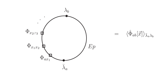
Figure 1: Disc diagram with two zero modes $\bar{\lambda}_{a}$ and $\lambda_{b}$ which change the boundary from the matter branes to the Ep-instanton brane. In addition matter fields $\Phi_{ij}$ are inserted. Between insertions $\Phi_{ij}$ and $\Phi_{jk}$ the boundary is the matter brane $j$.

The amplitude contains both an exponential of the the classical instanton action $S_{\rm inst}$ and of the vacuum one-loop partition function $Z_{\rm 1-loop}$ with at least one boundary on the instanton. This factor is nothing else than the one-loop determinant of fluctuations around the instanton background. In the case of an Ep-instanton, the classical instanton action is given by eq.(10).

Summarizing, D-brane instantons with the right number of zero modes generate contributions to the matter field superpotential of the following schematic form

$$W={1\over M_{P}^{n}}\int d^{4}x\,d^{2}\theta\;\prod_{i=1}^{n+3}\Phi_{a_{i}b_{i}}\;A(U)\;e^{-S_{Ep}}$$ (17)

where $A(U)$ is a moduli dependent one-loop determinant.

2.3 Loop dressing of instanton induced F-terms

It is a general feature of supersymmetric extensions of the Standard Model that new higher dimensional F-terms do not directly lead to new Standard Model processes, as only two of the external states are fermions and all the remaining ones are bosonic superpartners. Thus one has to dress these effective new interactions by additional loops, which convert the bosonic superpartners into the Standard Model fermionic matter particles. This is quite well known for supersymmetric dimension five proton decay operators and also for the supersymmetric FCNC operators of main interest in this paper. The standard field theory diagram of such a loop diagram is shown in figure 2.

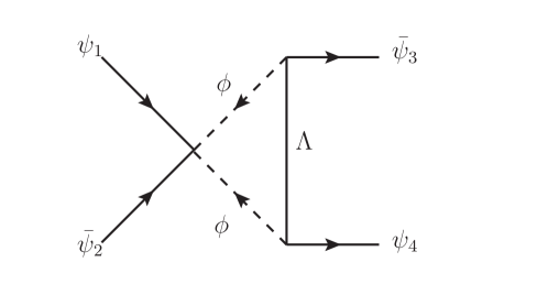
Figure 2: Coupling of the instanton contribution to the MSSM

For the external particles to be all fermions, the propagators in the loop must involve two bosonic and one fermionic superpartner of Standard Model particles. In the MSSM the two vertices on the right hand side must clearly satisfy the selection rules of the MSSM.

However, in string theory respectively intersecting D-brane realization of the MSSM, one has these additional global $U(1)$ symmetries, which all perturbative couplings have to satisfy. Therefore, in a concrete MSSM like D-brane model, not every MSSM diagram necessarily is present in string theory. In order to see directly what is possible, it is helpful to know the complete string theory diagram, i.e. the diagram which involves both the instanton induced higher dimensional F-term and the additional perturbative loop.

Thus, we are looking for an extension of the instanton calculus from the last section, which directly involves the loop. Cutting the above diagram by a vertical line going through the dimension five vertex, it is clear what we should do. As the left hand side involves the external particles and the instanton, it is just the usual absorption of charged instanton zero modes via disc diagrams, as discussed in the last section. Contrarily, the right hand side of the diagram involves the external particles and the instanton connected by a loop. Thus instead of absorbing the fermionic zero modes by disc diagrams, we do it by a one-loop annulus diagram as shown in figure 3. Since we have two fermionic matter zero modes on the annulus, this diagram does not contribute to the superpotential, which is of course consistent with the fact that the entire process is a dimension six operator with four external fermions.

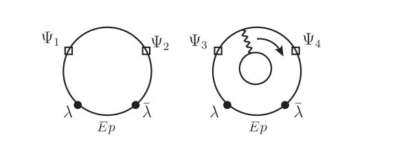
Figure 3: String theoretic realization of the process

The internal propagators can then easily be read off from the nature of the open strings stretching between the internal boundary and the various segments of the external boundary. Since this is a consistent string diagram, all selection rules are automatically satisfied. It is clearly not an easy task to compute the whole instanton diagrams, but for our purposes it is not necessary, as we are mainly interested in the selection rules.

What we have just discussed is the string theory diagram corresponding to a field theory diagram where a single vertex is non-perturbatively realized in string theory. Clearly, this can be generalized to the case that more than one field theory vertex is generated by instantons. In this case the whole diagram is a multi-instanton process in string theory and one has to integrate over all the appearing zero modes leading to a multi-exponential suppression. Without developing the whole formalism at this point, let us discuss an example, which shows the main features and will be relevant in the following. Let us assume that the upper right vertex $(\phi,\overline{\psi}_{3},\Lambda)$ in the field theory diagram in figure 2 is generated non-perturbatively by another Ep-instanton in string theory. Moreover, we assume this Yukawa interaction is generated by an instanton with six matter zero modes, so that in the instanton calculus one needs three disc diagram

$$\langle\Phi\rangle_{\lambda_{1}\overline{\lambda}_{1}},\quad\langle\Psi_{3}\rangle_{\lambda_{2}\overline{\lambda}_{2}},\quad\langle\Lambda\rangle_{\lambda_{3}\overline{\lambda}_{3}}$$ (18)

to absorb all matter zero modes. The question is, how all these three couplings can be put into the loop diagram in figure 3. Clearly, the change can only involve the closer environment of the $\overline{\psi}_{3}$ insertion. We propose that indeed the D-brane instanton calculus is rich enough to be able to also include such cases and that the annulus diagram in 3 is changed close to the $\overline{\psi}_{3}$ insertion in the way shown in figure 4.

Figure 4: non-perturbative Yukawa vertex: the dashed lines indicate cuts one can make in order to visualize the three disc diagrams (18)

Let us emphasize again that being able to write such diagrams directly in an extended instanton calculus in string theory ensure that all global $U(1)$ selection rules are automatically satisfied.

We will see that such diagrams appear for instanton induced higher dimensional F-terms and their one-loop conversion to observable amplitudes. We will use these diagrammatic techniques in our discussion of FCNCs in TeV scale D-brane models.

3 Flavor-violation in 5-stack quivers

So far our discussion has been quite general and more on the technical level. Let us now move forward to discuss the appearance of perturbative and non-perturbative FCNCs in intersecting D-brane models. In a bottom-up approach, quasi-realistic models of the MSSM in terms of intersecting branes were studied for example in [14] and [15]. In order to demonstrate how the techniques described so far can be utilized, we will concentrate on a very specific example, namely one of the promising looking five-stack models of [27].

3.1 The 5-stack quiver and its Yukawa couplings

Intersecting D-brane compactifications have the potential to realize the particles of the SM at low energies without chiral exotics. Specifically, open strings that are located on local D-brane quivers give rise to the SM degrees of freedom, where the D-brane quiver typically contains three, four, five or even more stacks of D-branes. As a demonstrative example, we will use in the following the 5-stack quiver, which was also recently investigated in [27] as a local model that comes close to the MSSM. In this model the hypercharge is given by the linear combination

$$U(1)_{Y}=\frac{1}{6}U(1)_{a}+\frac{1}{2}U(1)_{c}+\frac{1}{2}U(1)_{d}+\frac{1}{2}U(1)_{e}\;.$$ (19)

One choice of matter content is given in table 2.

Table 2: Spectrum of the 5-stack quiver

Sector	Matter	Representation	Multiplicity	Hypercharge
$ab$	$Q_{L}^{1}$	$(\bf{3},\bf{2})_{(1,-1,0,0,0)}$	$1$	$\frac{1}{6}$
$ab^{\prime}$	$Q_{L}^{2,3}$	$(\bf{3},\bf{2})_{(1,1,0,0,0)}$	$2$	$\frac{1}{6}$
$ac$	$D_{R}$	$(\bar{\bf{3}},\bf{1})_{(-1,0,1,0,0)}$	$3$	$\frac{1}{3}$
$ac^{\prime}$	$U_{R}^{1,2}$	$(\bar{\bf{3}},\bf{1})_{(-1,0,-1,0,0)}$	$2$	$-\frac{2}{3}$
$ae^{\prime}$	$U_{R}^{3}$	$(\bar{\bf{3}},\bf{1})_{(-1,0,0,0,-1)}$	$1$	$-\frac{2}{3}$
$bc$	$H_{u}$	$(\bf{1},\bf{2})_{(0,-1,1,0,0)}$	$1$	$\frac{1}{2}$
$bc^{\prime}$	$H_{d}$	$(\bf{1},\bf{2})_{(0,-1,-1,0,0)}$	$1$	$-\frac{1}{2}$
$bd^{\prime}$	$L^{1,2}$	$(\bf{1},\bf{2})_{(0,-1,0,-1,0)}$	$2$	$-\frac{1}{2}$
$be$	$L^{3}$	$(\bf{1},\bf{2})_{(0,1,0,0,-1)}$	$1$	$-\frac{1}{2}$
$cd^{\prime}$	$E_{R}^{1}$	$(\bf{1},\bf{1})_{(0,0,1,1,0)}$	$1$	$1$
$ce^{\prime}$	$E_{R}^{2,3}$	$(\bf{1},\bf{1})_{(0,0,1,0,1)}$	$2$	$1$

The quark and lepton Yukawa couplings have the following $U(1)$-charges :

$$Q_{L}^{1}U_{R}^{12}H_{u} 0,-2,0,0,0$$

$$Q_{L}^{1}U_{R}^{3}H_{u} 0,-2,1,0,-1$$

$$Q_{L}^{2,3}U_{R}^{1,2}H_{u} 0,0,0,0,0$$

$$Q_{L}^{2,3}U_{R}^{3}H_{u} 0,0,1,0,-1$$

$$Q_{L}^{1}D_{R}H_{d} 0,-2,0,0,0,$$

$$Q_{L}^{2,3}D_{R}H_{d} 0,0,0,0,0$$

$$L^{1,2}H_{d}E_{R}^{1} 0,-2,0,0,0$$

$$L^{1,2}H_{d}E_{R}^{2,3} 0,-2,,0,-1,1$$

$$L^{3}H_{d}E_{R}^{1} 0,0,0,1,-1$$

$$L^{3}H_{d}E_{R}^{2,3} 0,0,0,0,0$$ (20)

We observe that the quark Yukawa couplings $Q_{L}^{23}U_{R}^{23}H_{u}$ and $Q_{L}^{23}D_{R}H_{d}$ are realized perturbatively and are therefore not suppressed by the exponential factor coming from D-instantons. Thus $Q_{L}^{23}$ should be identified with the two heavier families. Similar arguments hold for the perturbatively realized lepton-Yukawa coupling $L^{3}H_{d}E_{R}^{23}$.

The other Yukawa couplings have to be realized non-perturbatively by D-instantons which have the right charges (and thus intersection structure). These instantons not only generate the missing Yukawa couplings but also (we have to sum over all possible configurations) give rise to other phenomenologically important couplings. In the following section we are going to investigate the consequences of these additional couplings on processes which are highly suppressed or even completely forbidden in the standard model. As usual in a bottom-up approach, we will always assume that the respective instantons are really present in the model, which for global intersecting D-brane models provide further severe constraints.

3.2 Non-perturbative higher dimensional operators

We now begin to investigate possible flavour violating effects in MSSM models. First, there are perturbatively allowed contributions to quark flavour mixing, as pointed out in [8]. They are of the four fermion-type and therefore suppressed by the square of the string mass scale $M_{s}$:

$$\frac{1}{M_{s}^{2}}\langle\bar{\psi}\psi\bar{\psi}\psi\rangle\;.$$ (21)

If in an MSSM-like model the two lightest families are realized by the same representation, these four-fermion operators can contribute to flavour mixing. In the systematic search for realistic MSSM orientifold models done in [15], in every model this is indeed the case. The strongest bounds come from neutral Kaon mixing and were calculated in [8]. It was found that in case the two lightest families are realized by the same representation, they give a lower bound on the string scale of $M_{s}>10^{3-4}$ TeV. Note that for low string scale models this bound is already quite severe and essentially rules out 1TeV scale D-brane models of this type. Thus for rescuing a TeV scale scenario, we need to assume that these perturbative couplings are absent. However, even then there is the danger that further exponentially suppressed non-perturbative, i.e. D-brane instanton induced, FCNC couplings do not lower the bounds sufficiently enough. The evaluation of these bounds is the central question of this section.

To illustrate this, consider first the famous flavour violating process $K^{0}\leftrightarrow\bar{K}^{0}$ with $\Delta S=2$. In the SM, this process is induced by the 1-loop box-diagram, which involves the exchange of two $W$-bosons that couple $SU(2)$ doublets. It corresponds to an effective, dimension six 4-fermion operator of the form

$${\cal L}_{K^{0}\leftrightarrow\bar{K}^{0}}\sim(\bar{s}_{L}d_{L})(\bar{s}_{L}d_{L})$$ (22)

Now, depending on how we define three different quark flavors, there are two ways to realize this 4-fermion operator by the fields in the table of the five stack model. The first realization is

$$(A):\qquad{\cal L}_{K^{0}\leftrightarrow\bar{K}^{0}}=(\bar{Q}_{L}^{2,3}Q_{L}^{2,3})(\bar{Q}_{L}^{2,3}Q_{L}^{2,3})\qquad\Delta Q_{b}=0$$ (23)

and the second one

$$(B):\qquad{\cal L}_{K^{0}\leftrightarrow\bar{K}^{0}}=(\bar{Q}_{L}^{2,3}Q_{L}^{1})(\bar{Q}_{L}^{2,3}Q_{L}^{1})\qquad\Delta Q_{b}=4\;.$$ (24)

Apparently, the operator (A) is invariant under all $U(1)$ symmetries and is therefore present perturbatively. However, if we assign the the two heavier families to $Q_{L}^{2,3}$, this operator does not induce $K^{0}\leftrightarrow\bar{K}^{0}$ oscillations, but rather $B_{s}^{0}\leftrightarrow\bar{B}_{s}^{0}$ oscillations. As a perturbative 4-point coupling this dimension six operator is suppressed by $M_{s}^{-2}$.

The operator (B) violates $U(1)_{b}$ of the five-stack model, as it has charge $\Delta Q_{b}=4$. The reason behind this is that one needs also the Cabbibo angle, when going from the quark flavor to the quark mass eigenstates. This means that $K_{0}\leftrightarrow\bar{K}_{0}$ implicitly also contains two off diagonal Yukawa couplings. Indeed, some of the entries in the quark Yukawa coupling matrix of the five-stack model are perturbatively allowed, others violate some of the $U(1)$ symmetries. Therefore, the $K_{0}\leftrightarrow\bar{K}_{0}$ operator (B) can only be generated non-perturbatively via D-instantons. As we have discussed, the suppression of this non-perturbative operator depends on how it is precisely generated by instantons and on the scenario how the MSSM is embedded.

Next we turn to the discussion of the holomorphic flavor violating operators, which arise from a D-instanton induced holomorphic superpotential. We are looking for a classification of all possible holomorphic chain products of matter fields which are possible insertions in disc amplitudes together with the charged zero modes coming from the intersection of the Yukawa-instantons with the matter branes. Combining them according to the zero mode structure of the instantons, we get the whole set of holomorphic operators (we did the analysis up to mass dimension 5) generated by the instantons. In the following, we list the most interesting results:

1. $0,-2,0,0,0$

   If the charges are realized with two zero modes $\lambda_{b},\lambda_{b}$ we get the following interesting dimension 5 operators:

   $$Q_{L}^{1}D_{R}U_{R}^{12}Q_{L}^{1} Q_{L}^{1}U_{R}^{12}D_{R}Q_{L}^{1}$$

   $$Q_{L}^{1}U_{R}^{12}E_{R}^{1}L^{12} H_{d}E_{R}^{23}U_{R}^{3}Q_{L}^{1}$$

   $$L^{12}E_{R}^{23}U_{R}^{12}Q_{L}^{1}\;.$$ (25)

   The second way to realize this charge structure is with four zero modes $\lambda_{b},\lambda_{b},\lambda_{c},\bar{\lambda}_{c}$. If we combine two discs with $\lambda_{b}\lambda_{b}$ and $\lambda_{c}\bar{\lambda}_{c}$ inserted, there will be no operators of mass dimension lower than or equal to 5. But if we take one disc with $\lambda_{b},\lambda_{c}$ and one with $\lambda_{b},\bar{\lambda}_{c}$ we get the following operators:

   $$Q_{L}^{1}U_{R}^{12}Q_{L}^{1}D_{R} Q_{L}^{1}U_{R}^{12}L^{12}E_{R}^{1}$$

   $$H_{d}Q_{L}^{1}U_{R}^{3}E_{R}^{23}\;.$$ (26)

2. $0,-2,1,0,-1$

   If we combine $\lambda_{b}\lambda_{b}$ with $\bar{\lambda}_{c}\lambda_{e}$ there are no operators of dimension smaller or equal to 5. Combining $\lambda_{b}\bar{\lambda}_{c}$ and $\lambda_{b}\lambda_{e}$ we get the following operators:

   $$Q_{L}^{1}D_{R}Q_{L}^{1}U_{R}^{3} L^{12}E_{R}^{1}Q_{L}^{1}U_{R}^{3}$$

   $$Q_{L}^{1}D_{R}H_{u}H_{d}\;.$$ (27)

3. $0,0,1,0,-1$

   If we take the direct realization of the charges via $\bar{\lambda}_{c}\lambda_{e}$ we get the following operators:

   $$D_{R}Q_{L}^{1}L^{3} H_{u}L^{3}$$

   $$E_{R}^{1}L^{12}Q_{L}^{23}U_{R}^{3} E_{R}^{23}U_{R}^{3}Q_{L}^{1}L^{3}\;.$$ (28)

   The first line would give dangerous R-parity violating couplings!

4. $0,-2,0,-1,1$

   Only the combination of discs with $\lambda_{b}\lambda_{d}$ and $\lambda_{b}\bar{\lambda}_{e}$ gives operators of dimension smaller or equal to 5. They are:

   $$L^{12}Q_{L}^{1}U_{R}^{12}E_{R}^{23} L^{12}H_{d}E_{R}^{23}$$ (29)

5. $0,0,0,1,-1$

   In this case, if we take the direct realization of the charges via $\bar{\lambda}_{d}\lambda_{e}$ we get the following operators:

   $$E_{R}^{1}U_{R}^{12}Q_{L}^{1}L^{12} E_{R}^{1}H_{d}Q_{L}^{23}U_{R}^{3}\;.$$ (30)

   For the second realization via $\bar{\lambda}_{d}\lambda_{e}\lambda_{c}\bar{\lambda}_{c}$ there are 3 different possibilities to distribute the zero modes. In the case of $\bar{\lambda}_{d}\lambda_{e}$ on the first and $\lambda_{c}\bar{\lambda}_{c}$ on the second disc there are no operators of dimension 5 or lower. The combination $\bar{\lambda}_{d}\lambda_{c}$ and $\lambda_{e}\bar{\lambda}_{c}$ also gives no interesting operators. Finally, the combination $\bar{\lambda}_{d}\bar{\lambda}_{c}$ and $\lambda_{e}\lambda_{c}$ gives the following operators:

   $$E_{R}^{1}L^{3}Q_{L}^{1}U_{R}^{12} E_{R}^{1}L_{3}H_{d}$$

   $$E_{R}^{1}U_{R}^{3}Q_{L}^{23}H_{d}\;.$$ (31)

3.3 Quark flavour violation

Let us now focus on the possible contributions to flavour changing processes in the quark sector. Here we concentrate on neutral meson mixing because this is very well studied experimentally. Consider the contribution $Q_{L}^{1}\,U_{R}^{12}\,Q_{L}^{1}\,D_{R}$ from eq.(1). Taking the F-term, it contains the following interaction (the tilde again denotes the superpartner to the fermion), as depicted in figure 5.

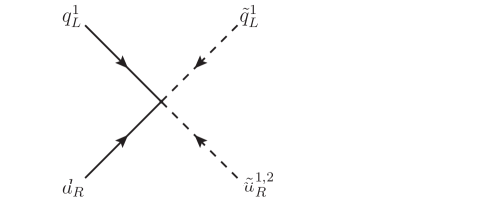
Figure 5: Instanton vertex: Solid lines represent fermions and dashed lines represent the bosonic superpartners
 

The strength of this vertex includes the instanton suppression factor and for dimensional reasons the inverse of the characteristic mass scale $M_{F}$, i.e. a scale between the string scale $M_{s}$ and the winding scale $M_{w}=M_{s}^{2/3}M_{p}^{1/3}$.

Next we discuss how to convert the holomorphic dimension five operator into a dimension six operator that involves four fermion fields. This can be done by inserting a Yukawa-coupling-vertex $\bar{Q}_{L}^{1}\bar{H}_{d}\bar{D}_{R}$ at the upper right and a vertex $\bar{Q}_{L}^{23}\bar{H}_{u}\bar{U}_{R}^{12}$ on the lower right. Thus we get as out-states the fermionic components of the superfields $\bar{D}_{R}$ and $\bar{Q}_{L}^{23}$. In addition, to complete the diagram we have to insert a $\mu$-term $\mu H_{d}H_{u}$. The first Yukawa coupling and the $\mu$-term are perturbatively forbidden and therefore need an instanton to be generated.

To realize the non-perturbative Yukawa coupling we use the techniques presented in section 2. The easiest possibility is to take the minimal amount of charged zero modes, i.e. $\lambda_{b},\lambda_{b}$. The disc and the corresponding piece in the annulus are given in figure 6.

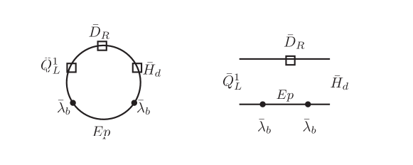
Figure 6: The non-perturbative Yukawa coupling and the corresponding piece in an annulus diagram

In the same way, we realize the $\mu$-term of the MSSM superpotential as part of an annulus diagram as given in figure 7.

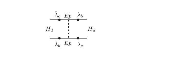
Figure 7: Realization of the $\mu$-term as part of an annulus

To close the annulus diagram, we combine the non-perturbative Yukawa coupling and the $\mu$-term with the perturbatively realized Yukawa coupling $\bar{Q}_{L}^{12}\bar{U}_{R}^{12}\bar{H}_{u}$. In addition, we insert the charged zero modes $\lambda_{b},\lambda_{c}$ at the inner boundary. As shown in figure 8, the whole three-instanton process has only standard model fermions as external states.

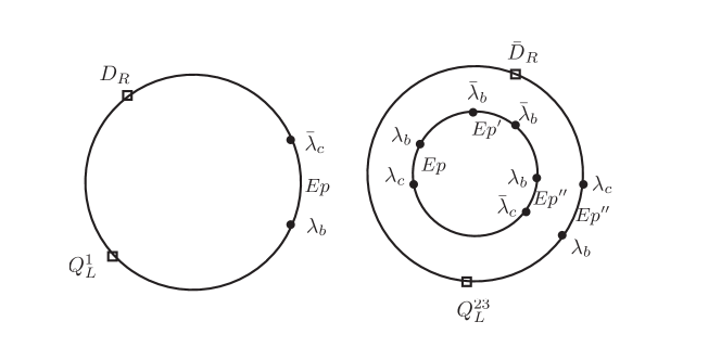
Figure 8: 3-instanton contribution to neutral Kaon mixing

If we now integrate out the charged zero modes, we get a connected diagram and taking the field theory limit (where $\alpha^{\prime}\rightarrow 0)$ we receive an MSSM process which contributes to neutral Kaon mixing (figure 9).

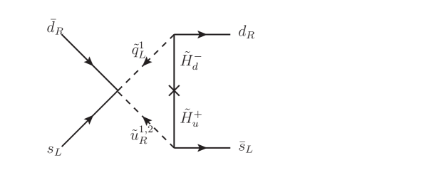
Figure 9: Coupling of the instanton contribution to the MSSM

Since we are interested in the order of magnitude of the process, we just estimate the characteristic contributions to the vertices and the propagators. The instanton suppression factors of the nonperturbative Yukawa-coupling and the $\mu$-term are fixed by the requirement to have the order of magnitude of the respective standard model/MSSM values. By this reasoning we obtain

$$\mathcal{M}\approx\frac{e^{-S_{0}}}{M_{F}}\frac{\mu~{}m_{\textrm{susy}}^{4}m_{K^{0}}^{2}}{m_{\tilde{q}_{L}^{1}}^{2}m_{\tilde{u}_{R}^{12}}^{2}m_{\tilde{H}}^{2}}\frac{m_{d}m_{s}}{m_{\textrm{weak}}^{2}}\;,$$ (32)

where we wrote a factor of $m_{x}^{2}$ for a propagator of a boson and $m_{x}$ for the propagator of a fermion. Moreover, we inserted a factor of the characteristic energy $m_{\textrm{susy}}^{4}$ coming from the loop integration. In addition there is a factor of the quark mass over the electroweak breaking scale coming from the respective Yukawa coupling and $\mu$ from the Higgs $\mu$-term. $M_{F}$ is the mass suppression of the physical dimension five operator. Finally we need a factor of $g_{s}^{4}$ (where $g_{s}$ is the string coupling) because we inserted 8 charged zero modes on an annulus, which comes with an overall normalization of $g_{s}^{0}$. The factor of $e^{-S_{0}}$ can also be expressed in terms of quark masses $m_{c}:m_{t}\approx\frac{1}{100}$ which is required to get the right family mass hierarchy. We are now going to estimate the contribution of this process to neutral Kaon mixing which can be seen experimentally in the mass difference $\Delta m$ of the $K_{L}^{0}$ and $K_{S}^{0}$ states. It is well known how to compute the mass difference from the effective 4-fermion operator of $K^{0}\leftrightarrow\bar{K}^{0}$-mixing: The evaluation of the operator between the $K^{0}$ eigenstates gives a factor of $\frac{8}{3}\frac{f_{K}^{2}m_{K}^{2}}{2m_{K}}$ ($f_{K}$ is the Kaon decay constant and $m_{K}$ is the Kaon mass) and together with the estimate of the amplitude this gives

$$\Delta m\approx\frac{e^{-S_{0}}}{M_{F}}\frac{\mu~{}m_{\textrm{susy}}^{4}}{m_{\tilde{q}_{L}^{1}}^{2}m_{\tilde{u}_{R}^{12}}^{2}m_{\tilde{H}}^{2}}\frac{m_{d}m_{s}}{m_{\textrm{weak}}^{2}}\frac{8}{3}\frac{f_{K}^{2}m_{K^{0}}^{2}}{2m_{K}}$$ (33)

This gives a contribution to the mass difference depending on the string mass of the order

$$\Delta m\approx\frac{1}{M_{F}}10^{-21}\,\textrm{TeV}^{2}\;.$$ (34)

Now the experimental accuracy of measurements of the mass difference is of the order $10^{-21}$ TeV which for $M_{F}=M_{w}$ leads to a lower bound on the string scale of

$$M_{s}\geq 10^{-7}\,\textrm{TeV}.$$ (35)

This is not very restrictive. The first reason for this is the high suppression of the three-instanton amplitude due to the down- and strange- quark Yukawa couplings. In addition the winding scale factor $M_{w}$ gives a suppression of the order of $M_{P}^{1/3}$. Contrarily, for $M_{F}=M_{s}$ we get a lower bound on the string scale of the order of

$$M_{s}\geq 1\,\textrm{TeV},$$ (36)

which is significantly larger. Finally the result also depends on the experimental accuracy of $\Delta m$ measurements and can give stronger bounds in the future.

3.4 Lepton flavour violation

In the standard model with massless neutrinos, we have conserved lepton flavour number. Thus every observation of lepton-flavour violating (LFV) processes would be a definite hint for physics beyond the standard model. The most precise bounds on possible LFV processes come from the Kaon and D-meson systems. In the following we list the most promising candidate decay processes (the branching ratio BR gives the ratio of the decay rate of the process to the total decay rate of the initial meson).

Table 3: Kaon decays into standard model particles with BR $<5\cdot 10^{-10}$ [28]

Decay	Branching ratio
$K_{L}^{0}\rightarrow\mu^{\pm}e^{\mp}$	$<4.7\cdot 10^{-12}$
$K^{+}\rightarrow\pi^{+}\mu^{+}e^{-}$	$<2.8\cdot 10^{-11}$
$K_{L}^{0}\rightarrow\pi^{0}\mu^{+}e^{-}$	$<4.4\cdot 10^{-10}$
$K^{+}\rightarrow\pi^{-}\mu^{+}e^{+}$	$<5.0\cdot 10^{-10}$

Table 4: Examples for decay modes of $D^{0}$ with BR$<5\cdot 10^{-6}$ [29]

Decay	Branching ratio
$D^{0}\rightarrow e^{+}e^{-}$	$<0.6\cdot 10^{-6}$
$D^{0}\rightarrow\mu^{+}\mu^{-}$	$<3.4\cdot 10^{-6}$
$D^{0}\rightarrow\mu^{\pm}e^{\mp}$	$<1.9\cdot 10^{-6}$

The list of higher dimensional operators from section 3.2 reveals the existence of various interesting operators, which contain two quark and two lepton fields and therefore could contribute to one of the meson decays of the table. Taking the operator

$$Q_{L}^{1}U_{R}^{12}E_{R}^{1}L^{12}$$ (37)

we again get a specific combination of a disc with an annulus which is given in figure 10. There are the following particles running in the loop (we use our example quiver of table 2): The $bd^{\prime}$-sector corresponds to a lepton $L$, $dd^{\prime}$ is a gauge boson (photon) or its superpartner and the $dc$-sector corresponds to $E_{R}^{1}$. Therefore, in field theory the process would correspond to the Feynman diagram given in figure 11. To get proper MSSM couplings with standard model fermions as out-states, we get superpartners running in the loop: In our case sleptons $\tilde{L}$ and $\tilde{E}_{R}^{1}$ and the photino $\tilde{\gamma}$. The whole process would therefore contribute to the following decays of the $D^{0}$-meson:

$$D^{0}\rightarrow e^{-}e^{+}\,,\quad D^{0}\rightarrow\mu^{-}e^{+}\,.$$ (38)

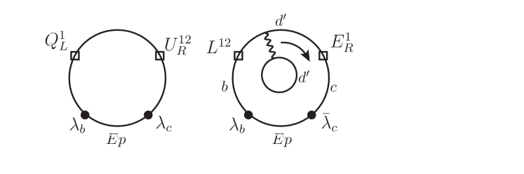
Figure 10: Instanton contribution to $D^{0}$-decay

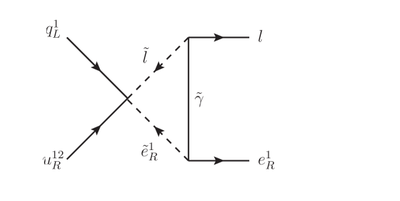
Figure 11: Instanton contribution to $D^{0}$-decay in the field theory limit

Let us now estimate the order of magnitude of this process in field theory, as given in figure 11. From the instanton vertex we get the suppression factor $\frac{e^{-S_{0}}}{M_{F}}$ . From the loop integration we get a factor of $m_{\textrm{susy}}^{4}$. Together with the propagator masses, the electromagnetic coupling constant and using as kinematical factor the mass of the initial state of the $D^{0}$ we get

$$\mathcal{M}\propto\frac{e^{-S_{0}}}{M_{F}}m_{\textrm{susy}}^{4}\frac{m_{D^{0}}^{2}}{m_{\textrm{susy}}^{5}}g_{\textrm{em}}^{2}(m_{\textrm{susy}})$$ (39)

Using $1\textrm{TeV}$ for the supersymmetry scale, $\frac{1}{100}$ for the instantonic suppression (which is set by the ratio of the heaviest quark to the charm quark) and the mass of the $D^{0}$ (2GeV), we get as a rough estimate

$$\mathcal{M}\propto 4\cdot 10^{-9}\frac{\textrm{TeV}}{M_{F}}$$ (40)

We want to compare this to the experimental bound for the above given $D^{0}$-decays. The lifetime of the $D^{0}$ is $\tau_{D^{0}}=4,1\cdot 10^{-13}sec$, which leads to (using the branching ratio given in table 6.3) a decay rate of

$$\Gamma_{D^{0}\rightarrow LE_{R}^{1}}=\textrm{BR}(D^{0}\rightarrow LE_{R}^{1})\Gamma_{D^{0}}<10^{-18}\textrm{GeV}.$$ (41)

Now the amplitude of the process can be estimated by using

$$\Gamma_{D^{0}\rightarrow LE_{R}^{1}}\approx m_{D^{0}}|\mathcal{M}|^{2}$$ (42)

The result is $|\mathcal{M}|<10^{-9}$. Comparing this with the field theory estimate of the instanton process (and assuming $M_{F}=M_{w}$) we get a lower bound on the string scale of order

$$M_{s}\geq 10^{-7}\textrm{TeV}$$ (43)

which is certainly not very restrictive.

We see that the winding factor gives us an additional very high suppression factor such that instanton contributions to meson decay are very weak. To illustrate this, we skip this and calculate only with the naive expectation of a suppression of $M_{F}=M_{s}$ characteristic for effective dimension 5 operators, i.e. we have

$$\mathcal{M}\propto\frac{e^{-S_{0}}}{M_{s}}m_{\textrm{susy}}^{4}\frac{m_{D^{0}}^{2}}{m_{\textrm{susy}}^{5}}g_{\textrm{em}}^{2}(m_{\textrm{susy}})=4\cdot 10^{-9}\frac{\textrm{TeV}}{M_{s}}\,.$$ (44)

This would lead to the lower bound of

$$M_{s}\geq 4\textrm{TeV}.$$ (45)

Another important fact is that the experimental bounds on the $D^{0}$-decay are not as good as for Kaon decays. If we possibly had future experimental bounds similar to Kaon decays (table 3), we would get $M_{s}>3\cdot 10^{-3}$ TeV with winding scale and $M_{s}>4\cdot 10^{3}$ TeV without this scale.

A process which is restricted much more by experiment is the LFV Kaon decay

$$K^{0}\rightarrow e^{+}\mu^{-}$$ (46)

We propose that this process gets contributions from a 3-instanton process. To show this, we take the operator $Q_{L}^{1}U_{R}^{12}E_{R}^{1}L^{12}$ found in eq.(1). Similar to the contribution to neutral Kaon mixing discussed in the last section we combine a disc and an annulus diagram (figure 12). Two of the zero modes which are needed to generate the operator are inserted in the disc and the other two in the annulus, and therefore we get again a connected diagram after the integration over the zero modes. In the field theory limit this corresponds to the process given in figure 13.

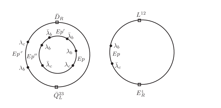
Figure 12: 3-instanton contribution to the LFV Kaon decay

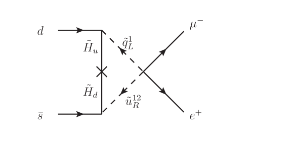
Figure 13: Instanton contribution to $K^{0}\rightarrow e^{+}\mu^{-}$

Let us also determine the order of magnitude of this process. If we use the same estimates as for neutral Kaon mixing and $D^{0}$-decay we get the following for the amplitude:

$$\mathcal{M}\propto\frac{e^{-S_{0}}}{M_{F}}\frac{\mu~{}m_{\textrm{susy}}^{4}m_{K^{0}}^{2}}{m_{\textrm{susy}}^{4}m_{\textrm{susy}}^{2}}\frac{m_{d}m_{s}}{m_{weak}^{2}}$$ (47)

In addition to the estimate for $D^{0}$ we use here the $\mu$-term which we assume to be of the order of the supersymmetry scale and we used the standard model values for the Yukawa couplings which are of the order of $\frac{m_{\textrm{quark}}}{m_{\textrm{weak}}}$, where $m_{\textrm{weak}}$ is the electroweak breaking scale.

Taking again the same estimate for the instanton suppression factor we get for the estimate of the amplitude $\mathcal{M}\propto 10^{-12}$ and a bound on the string scale of the order

$$M_{s}\geq 10^{-12}\textrm{TeV}$$ (48)

This is clearly not a bound on the string scale at all. Again the extreme suppression of the amplitude can be explained by the two light Yukawa couplings included in the 3-instanton process and the contribution of the winding scale factor.

In the following table 5 we compare the perturbative bound [8] with the instanton results from $D^{0}$-decay (first line with the real experimental upper bound, and second line with a hypothetical bound comparable to Kaon decay) and with the results for LFV Kaon decays (third line) and neutral Kaon mixing (fourth line). These could become important in MSSM models, for which there is no tree level perturbative contribution, and hence instanton contributions to lepton flavour violating Kaon decays are dominant. To emphasize the importance of the winding factor we list the results with and without this factor.

Table 5: Comparison of the results for the string scale

Process	Perturbative	Winding	No winding
$D^{0}\rightarrow LE_{R}^{1}$	-	$10^{-7}$ TeV	$4$ TeV
$D^{0}\rightarrow LE_{R}^{1}$	-	$10^{-3}$ TeV	$4\cdot 10^{3}$ TeV
$K_{L}^{0}\rightarrow\mu^{-}e^{+}$	$100$ TeV	$10^{-12}$ TeV	$10^{-2}$ TeV
$K^{0}\leftrightarrow\bar{K}^{0}$	$10^{3}$ TeV	$10^{-7}$ TeV	$1$TeV

We conclude that the results using $D^{0},K^{0}$-decay and neutral Kaon mixing with today’s experimental bounds are not very restrictive, especially in comparison to results from perturbative allowed operators. However, for models which do not allow such operators and also would give rise to non-perturbative Kaon or D-meson decay operators the above results would give restrictions on the string mass.

4 Conclusion and outlook

In this paper we have considered instanton induced FCNC couplings in (softly broken) supersymmetric intersecting D-brane models. Technically, the relevant field theory diagrams involve dimension five F-terms dressed by an additional loop to convert the bosonic squarks and sleptons to fermionic matter particles. We have seen that in string theory the corresponding diagrams can be consistently described in an extended multi-instanton calculus, which involved disc and annulus diagrams with a mixture of space-time filling and instantonic D-brane boundaries with the appropriate insertions of (boundary changing) matter and instanton zero modes. We did not provide the full formalism but discussed this for a couple of relevant examples.

Equipped with these techniques we considered a concrete five stack MSSM-like intersecting D-brane model and found that experimentally highly suppressed FCNC processes like $K^{0}-\overline{K}^{0}$ mixing and leptonic meson decays are generated by (multi-) D-brane instantons. The appearing exponential suppression factors could be estimated due to the fact that the corresponding instantons also induced perturbatively forbidden Yukawa couplings. We computed and compared the appearing bounds on the string scales for two reasonable mass scales of the physical dimension five operators. For this latter scale being of the order of the string scale, one finds bounds of the order $1-4\,$TeV, which are of similar size as the bounds for perturbative dimension six operators. However, for quiver type MSSMs the suppression scale is rather the significantly larger winding scale, which only give extremely mild lower bounds on the string scale. Moreover, for processes involving more than one instanton, like neutral Kaon mixing and the LVF Kaon decay we get additional high suppression due to the light quark Yukawa couplings generated by D-instantons.

We conclude that, if there exist MSSM models which avoid perturbative allowed FCNC operators such as $Q_{L}\bar{Q}_{L}Q_{L}\bar{Q}_{L}$ or $D_{R}\bar{D}_{R}D_{R}\bar{D}_{R}$ (which would be very attractive for a string model in the range of the LHC), instanton contributions can become important and, depending on the mass scale of the dimension five operators, can provide non-negligible lower bounds on the string scale.

Acknowledgement

R. Blumenhagen and D. Lüst would like to thank the Kavli Institute for Theoretical Physics, Santa Barbara for the hospitality during part of this work. This research was supported in part by the National Science Foundation under Grant No. PHY05-51164.

References

- [1] R. Blumenhagen, B. Körs, D. Lüst and S. Stieberger, “Four-dimensional String Compactifications with D-Branes, Orientifolds and Fluxes,” Phys. Rept. 445, 1 (2007) [arXiv:hep-th/0610327].
- [2] D. Lüst, S. Stieberger and T. R. Taylor, “The LHC String Hunter’s Companion,” Nucl. Phys. B 808, 1 (2009) [arXiv:0807.3333 [hep-th]].
- [3] D. Lüst, O. Schlotterer, S. Stieberger and T. R. Taylor, “The LHC String Hunter’s Companion (II): Five-Particle Amplitudes and Universal Properties,” Nucl. Phys. B 828, 139 (2010) [arXiv:0908.0409 [hep-th]].
- [4] L. A. Anchordoqui, H. Goldberg and T. R. Taylor, “Decay widths of lowest massive Regge excitations of open strings,” Phys. Lett. B 668, 373 (2008) [arXiv:0806.3420 [hep-ph]].
- [5] L. A. Anchordoqui, H. Goldberg, D. Lüst, S. Nawata, S. Stieberger and T. R. Taylor, “Dijet signals for low mass strings at the LHC,” Phys. Rev. Lett. 101, 241803 (2008) [arXiv:0808.0497 [hep-ph]].
- [6] L. A. Anchordoqui, H. Goldberg, D. Lüst, S. Nawata, S. Stieberger and T. R. Taylor, “LHC Phenomenology for String Hunters,” Nucl. Phys. B 821, 181 (2009) [arXiv:0904.3547 [hep-ph]].
- [7] S. Cullen, M. Perelstein and M. E. Peskin, “TeV strings and collider probes of large extra dimensions,” Phys. Rev. D 62, 055012 (2000) [arXiv:hep-ph/0001166].
- [8] S. A. Abel, M. Masip and J. Santiago, “Flavour changing neutral currents in intersecting brane models,” JHEP 0304, 057 (2003) [arXiv:hep-ph/0303087].
- [9] R. Blumenhagen, M. Cvetic and T. Weigand, “Spacetime instanton corrections in 4D string vacua - the seesaw mechanism for D-brane models,” Nucl. Phys. B 771, 113 (2007) [arXiv:hep-th/0609191].
- [10] L. E. Ibanez and A. M. Uranga, “Neutrino Majorana masses from string theory instanton effects,” JHEP 0703, 052 (2007) [arXiv:hep-th/0609213].
- [11] R. Blumenhagen, M. Cvetic, D. Lüst, R. Richter and T. Weigand, “Non-perturbative Yukawa Couplings from String Instantons,” Phys. Rev. Lett. 100, 061602 (2008) [arXiv:0707.1871 [hep-th]].
- [12] B. Florea, S. Kachru, J. McGreevy and N. Saulina, “Stringy Instantons and Quiver Gauge Theories,” JHEP 0705 (2007) 024 [arXiv:hep-th/0610003].
- [13] R. Blumenhagen, M. Cvetic, S. Kachru and T. Weigand, “D-Brane Instantons in Type II Orientifolds,” Ann. Rev. Nucl. Part. Sci. 59 (2009) 269 [arXiv:0902.3251 [hep-th]].
- [14] P. Anastasopoulos, E. Kiritsis and A. Lionetto, “On mass hierarchies in orientifold vacua,” JHEP 0908 (2009) 026 [arXiv:0905.3044 [hep-th]].
- [15] M. Cvetic, J. Halverson and R. Richter, “Realistic Yukawa structures from orientifold compactifications,” JHEP 0912 (2009) 063 [arXiv:0905.3379 [hep-th]].
- [16] R. Blumenhagen, M. Cvetic, R. Richter and T. Weigand, “Lifting D-Instanton Zero Modes by Recombination and Background Fluxes,” JHEP 0710, 098 (2007) [arXiv:0708.0403 [hep-th]].
- [17] I. Garcia-Etxebarria and A. M. Uranga, “Non-perturbative superpotentials across lines of marginal stability,” JHEP 0801, 033 (2008) [arXiv:0711.1430 [hep-th]].
- [18] J. P. Conlon, D. Cremades and F. Quevedo, “Kaehler potentials of chiral matter fields for Calabi-Yau string compactifications,” JHEP 0701 (2007) 022 [arXiv:hep-th/0609180].
- [19] J. P. Conlon and D. Cremades, “The neutrino suppression scale from large volumes,” Phys. Rev. Lett. 99 (2007) 041803 [arXiv:hep-ph/0611144].
- [20] J. P. Conlon and E. Palti, “On Gauge Threshold Corrections for Local IIB/F-theory GUTs,” Phys. Rev. D 80, 106004 (2009) [arXiv:0907.1362 [hep-th]].
- [21] J. P. Conlon and F. G. Pedro, “Moduli Redefinitions and Moduli Stabilisation,” arXiv:1003.0388 [hep-th].
- [22] M. Billo, M. Frau, I. Pesando, F. Fucito, A. Lerda and A. Liccardo, “Classical gauge instantons from open strings,” JHEP 0302 (2003) 045 [arXiv:hep-th/0211250].
- [23] R. Argurio, M. Bertolini, G. Ferretti, A. Lerda and C. Petersson, “Stringy Instantons at Orbifold Singularities,” JHEP 0706, 067 (2007) [arXiv:0704.0262 [hep-th]].
- [24] M. Bianchi, F. Fucito and J. F. Morales, “D-brane Instantons on the orientifold,” JHEP 0707, 038 (2007) [arXiv:0704.0784 [hep-th]].
- [25] L. E. Ibanez, A. N. Schellekens and A. M. Uranga, “Instanton Induced Neutrino Majorana Masses in CFT Orientifolds with MSSM-like spectra,” JHEP 0706, 011 (2007) [arXiv:0704.1079 [hep-th]].
- [26] N. Akerblom, R. Blumenhagen, D. Lust and M. Schmidt-Sommerfeld, “Instantons and Holomorphic Couplings in Intersecting D-brane Models,” JHEP 0708, 044 (2007) [arXiv:0705.2366 [hep-th]].
- [27] M. Cvetic, J. Halverson, P. Langacker and R. Richter, “The Weinberg Operator and a Lower String Scale in Orientifold Compactifications,” arXiv:1001.3148 [hep-th].
- [28] A. R. Barker and S. H. Kettell, “Developments in Rare Kaon Decay Physics,” Ann. Rev. Nucl. Part. Sci. 50 (2000) 249 [arXiv:hep-ex/0009024].
- [29] G. Burdman and I. Shipsey, “ - mixing and rare charm decays,” Ann. Rev. Nucl. Part. Sci. 53 (2003) 431 [arXiv:hep-ph/0310076].