Metastability in a nano-bridge based hysteretic DC-SQUID embedded in superconducting microwave resonator

Abstract

We study the metastable response of a highly hysteretic DC-SQUID made of a Niobium loop interrupted by two nano-bridges. We excite the SQUID with an alternating current and with direct magnetic flux, and find different stability zones forming diamond-like structures in the measured voltage across the SQUID. When such a SQUID is embedded in a transmission line resonator similar diamond structures are observed in the reflection pattern of the resonator. We have calculated the DC-SQUID stability diagram in the plane of the exciting control parameters, both analytically and numerically. In addition, we have obtained numerical simulations of the SQUID equations of motion, taking into account temperature variations and non-sinusoidal current-phase relation of the nano-bridges. Good agreement is found between experimental and theoretical results.

I Introduction

In the last two decades Superconducting Quantum Interference Devices (SQUIDs) have regained the interest of researchers worldwide, due to their use as solid-state quantum bits. More recently, such SQUIDs were embedded in superconducting Transmission Line Resonators (TLRs), in order to produce circuit cavity quantum electrodynamics in the strong Chiorescu et al. (2004); Johansson et al. (2006); Houck et al. (2007); Majer et al. (2007); Sillanpaa et al. (2007); Astafiev et al. (2010a) and the dispersive Lupascu et al. (2006); Lee et al. (2007); Lupascu et al. (2004) coupling regimes Schoelkopf and Girvin (2008). Other applications, in which SQUIDs are mainly used as nonlinear classical elements, include Josephson bifurcation amplifiers Mallet et al. (2009); Bergeal et al. (2010); Vijay et al. (2009); Astafiev et al. (2010b) and tunable resonators Sandberg et al. (2008); Castellanos-Beltran and Lehnert (2007); Palacios-Laloy et al. (2008). Tunable resonators were also used to demonstrate parametric amplification and squeezing Castellanos-Beltran et al. (2008, 2009); Thol n et al. (2009); Yamamoto et al. (2008), and might also be used to demonstrate the dynamical Casimir effect Johansson et al. (2009); Wilson et al. (2010).

The injected power into a TLR is usually limited by the critical current of the DC-SQUID embedded in the resonator. The upper bound of this current is determined by the sum of the two critical currents of the Josephson junctions (JJs) composing the DC-SQUID. While typical critical currents of DC-SQUIDs range between few to tenth of microamperes, the applications that involve resonance tuning and parametric amplification could benefit from larger critical currents. In order to have larger critical currents one can fabricate DC-SQUIDs using nano-bridges instead of JJs. Nano-bridges, which are merely artificial weak-links having sub-micron size, were shown to have similar Current-Phase Relationship (CPR) as JJs under certain conditions Likharev (1979); Troeman et al. (2008); Hasselbach et al. (2002). These nano-bridge JJs (NBJJs) are characterized by large critical current, on the order of milliamperes Troeman et al. (2007); Hao et al. (2009). DC-SQUIDs with large critical currents are often characterized by hysteretic response and metastable dynamics Tesche and Clarke (1977); Matsinger et al. (1978a); Lefevre-Seguin et al. (1992); Goldman et al. (1965); Palomaki et al. (2006). These characters are naturally made extreme in NBJJ based DC-SQUIDs. In addition, NBJJs have very high plasma frequency Suchoi et al. (2010), on the order of one Terahertz, which enables operation of the microwave TLR without introducing interstate transitions in the embedded SQUID. Thus one could employ a SQUID as a nonlinear lumped inductor, operating at microwave frequencies.

In this paper we experimentally and numerically study metastable response of NBJJs based DC-SQUID, subjected to an alternating biasing current. We first theoretically analyze stability zones of a highly hysteretic DC-SQUID in the plane of the bias current and magnetic flux control parameters. Then we directly measure the voltage across a SQUID in that plane. Comparison between experimental results and between analytical and numerical theoretical predictions yields good agreement. Moreover, we measure the reflection spectra from several devices integrating a SQUID and a TLR and find qualitative agreement between the theory and the experiments.

II Experimental Setup

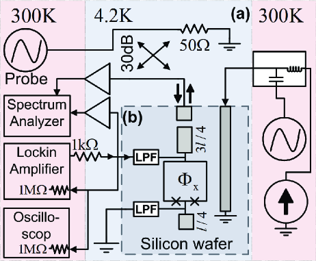
Figure 1: (Color online) $\mathrm{(a)}$ Measurement setup. $\mathrm{(b)}$ Schematic (unscaled) layout of our device. Red and blue background colors indicate experimental setup having temperatures of $300\operatorname{K}$ and $4.2\operatorname{K}$, respectively.

A simplified circuit layout of our devices is illustrated in Fig. 1$\mathrm{(b)}$. We fabricate our devices on high resistivity Silicon wafers, each covered by a thin layer of Silicon Nitride. Each device is made of Niobium, having layer thickness of less than $100\operatorname{nm}$, and is composed of a stripline resonator having a DC-SQUID embedded in its structure. The resonator is designed to operate in the gigahertz range, having a length of about $l=19\operatorname{mm}$, which sets its first resonance mode around $2.5\operatorname{GHz}$. The DC-SQUID has two NBJJs, one NBJJ in each of its two arms (see Fig. 2$\mathrm{(b)}$ and inset of Fig. 3). The NBJJs are fabricated using FEI Strata $400$ focused ion beam system Hao et al. (2007); Troeman et al. (2007) at an accelerating voltage of $30\operatorname{kV}$ and Gallium ions current of $1.5\mathrm{pA}$. The outer dimensions of the bridges range from $100\times 100\operatorname{nm}^{2}$ for large junctions to $60\times 80\operatorname{nm}^{2}$ for relatively small junctions. The actual dimensions of the weak-links are smaller because the bombarding Gallium ions penetrate into the Niobium layer, and consequently suppress superconductivity over a depth estimated between $30\operatorname{nm}$ and $50\operatorname{nm}$ Troeman et al. (2007); Datesman et al. (2005); Tettamanzi et al. (2009). Despite the small dimensions of our NBJJs, most of our SQUIDs have critical currents on the order of milliamperes (see table 1). A feed-line, weakly coupled to the resonator, is employed for delivering input and output signals. An on-chip transmission line passes near the DC-SQUID and is used to apply magnetic flux through the DC-SQUID at frequencies ranging from DC to the gigahertz. An on-chip filtered DC bias line is connected directly to the DC-SQUID and is used for direct measurements of the SQUID. The Low-Pass Filters (LPFs) are designed to minimize the degrading effect of these connections on the quality factor of the resonator. Some measurements are carried out while the device is fully immersed in liquid Helium, while others are carried out in a dilution refrigerator where the device is in vacuum. Further design considerations and fabrication details can be found elsewhere Segev et al. (2009); Suchoi et al. (2010).

Parameter	E19	E38	E42
SQUID Type	RF	DC	DC
SQUID Area $[\operatorname{\mu m}^{2}]$	$1936$	$870$	$1057$
Nb Thickness $[\mathrm{nm}]$	$50$	$100$	$60$
Self-Inductance $[\mathrm{pH}]$	$127$	$112$	$141$
$I_{\mathrm{c}}[\mathrm{mA}_{\mathrm{RMS}}]$	—	$2.29$	$1.74$
$\beta_{\mathrm{L}}$ Calc	—	$1089$	$106$
$\beta_{\mathrm{L}}$ Fit	—	$722$	$83$
$\widetilde{\beta}_{\mathrm{L}}$ Fit	$1.5$	—	$45,35$
$\alpha$ Fit	—	$0.026$	$0.032$

Table 1: SQUIDs parameters. The self-inductance was numerically calculated using FastHenry computer program Kam . The parameter $\beta_{\mathrm{L}}$ Calc was evaluated analytically using the measured critical current. The parameters $\beta_{\mathrm{L}}$ Fit, $\widetilde{\beta_{L}}$ Fit, and $\alpha$ Fit were evaluated according to fittings of stability diagrams to measured data.

The experimental results in this paper are obtained from three devices whose parameters are summarized in table 1. The experiments are carried out using the setup depicted in Fig. 1$\mathrm{(a)}$. We report on two types of experiments. In the first one we obtain low frequency current-voltage measurements of the SQUID using the DC bias line, while the resonator does not play any role. We use a lock-in amplifier, which applies alternating current through the SQUID, having excitation frequencies on the order of kilohertz. We measure the voltage across the SQUID using the lock-in amplifier and, in addition, we record the spectral density of the voltage using a spectrum analyzer and its time domain dynamics using an oscilloscope. In the second type of experiments we investigate the response of an integrated SQUID-TLR device to a monochromatic incident probe tone that drives one of the resonance modes of the TLR. The reflected power spectrum is recorded by a spectrum analyzer. In such experiments the DC bias line is left floating, and does not play any role in the measurement. In both types of experiments we apply DC magnetic flux through the SQUID, and in experiments with TLRs we also add modulated magnetic flux at gigahertz frequencies.

Numerical method

Simulations of DC-SQUID circuit model (see Fig. 2$\mathrm{(a)}$) are done by numerically integrating its Equations Of Motion (EOMs); Eqs. (7) and (8). We introduce a sinusoidal excitation current to the EOMs and calculate the phases of the two NBJJs composing the DC-SQUID, the DC-SQUID voltage versus time, and the Fourier transform of this voltage at the frequency of excitation. The experimental measurement frequency was usually in the order of $1\operatorname{kHz}$, which is about nine orders of magnitude smaller than the SQUID plasma frequency, and about six orders of magnitude smaller than the time-scale of thermal processes in the SQUID Tarkhov et al. (2008). Therefore, in order to make the simulations feasible in terms of computation time, we have made two ease assumptions. The first assumption is that the excitation frequency used in simulation can be increased as long as the DC-SQUID follows this excitation adiabatically. Adiabatic approximation of NBJJs based DC-SQUID is thoroughly analyzed in Ref. Suchoi et al. (2010), where it is shown that the plasma frequency of a NBJJs based DC-SQUID is expected to be in the order of $1\operatorname{THz}$. Thus in practice, the excitation frequency used in simulation is set between $100\operatorname{MHz}$ and $1\operatorname{GHz}$. The second assumption is that thermal processes have a negligible influence on the experimentally measured dynamics of the SQUID, as long as the excitation frequency is kept low. Therefore, although we use high excitation frequency in the simulations according to the first assumption, the temperature of the SQUID is held at base temperature and does not evolve with the SQUID dynamics. On the other hand, in simulations related to measurements done with an integrated TLR-SQUID device, is which the measurement frequency is high, thermal effects are taken into account by including thermal EOMs; Eq. (16).

III Theory of Hysteretic DC-SQUID

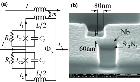
Figure 2: $\mathrm{(a)}$ Circuit model of a DC-SQUID. $\mathrm{(b)}$ Scanning electron microscope (SEM) image of a nano-bridge, whose dimensions are $80\times 60\times 50\operatorname{nm}^{3}$.

In this section, we develop a theory of hysteretic and metastable DC-SQUID, taking into account the self-inductance and asymmetry of the DC-SQUID. Similar models were also developed by others, but usually lacking comparison with experimental data Tesche and Clarke (1977); Goldman et al. (1965); Zahn (1981); Tsang and Duzer (1975); Palacios et al. (2006); Matsinger et al. (1978b); Ben-Jacob et al. (1983) or the emphasis put on other aspects of SQUID dynamics Lefevre-Seguin et al. (1992); Inchiosa et al. (1999); Wiesenfeld et al. (2000). We begin with a lossless model, in order to extract the SQUID stability diagram, and add the dissipation and fluctuation terms to the EOMs on a later stage.

The circuit model is shown in Fig. 2$\mathrm{(a)}$ (a SEM image can be seen in the inset of Fig. 3). It contains a DC-SQUID having two NBJJs, one in each of its arms, with critical currents $I_{\mathrm{c}1}$ and $I_{\mathrm{c}2}$, which in general may differ one from another. Both NBJJs are assumed to have the same shunt resistance $R_{\mathrm{J}}$ and capacitance $C_{\mathrm{J}}$ (which is considered extremely small for NBJJs Ralph et al. (1996)). The self-inductance of DC-SQUID, $L$, is assumed to be equally divided between its two arms. Typical inductance values of our SQUIDs are listed in table 1.

The DC-SQUID is controlled by two external parameters. The first is bias current $I_{\mathrm{x}}=I_{1}+I_{2}$, where $I_{1}$ and $I_{2}$ are the currents flowing in the upper and lower arms respectively (Fig. 2$\mathrm{(a)}$). The second is external magnetic flux $\Phi_{\mathrm{x}}$ applied through the DC-SQUID. The total magnetic flux threading the DC-SQUID loop is given by $\Phi=\Phi_{\mathrm{x}}+LI_{-},$where $I_{-}=\left(I_{1}-I_{2}\right)/2\;$is circulating current in the loop. Assuming sinusoidal CPR, the Josephson current $I_{\mathrm{J}k}$ in each junction ($k=1,2$) is related to the critical current $I_{\mathrm{c}k}$ and to the Josephson phase $\gamma_{k}$ by the Josephson equation $I_{\mathrm{J}k}=I_{\mathrm{c}k}\sin\gamma_{k}$. By employing the coordinate transformation $\gamma_{+}=\left(\gamma_{1}+\gamma_{2}\right)/2$ and $\gamma_{-}=\left(\gamma_{1}-\gamma_{2}\right)/2$, and the notation $I_{\mathrm{c}}=\left(I_{\mathrm{c}1}+I_{\mathrm{c}2}\right)$ and $I_{\mathrm{c}-}=\left(I_{\mathrm{c}1}-I_{\mathrm{c}2}\right)$, one finds that the potential governing the dynamics of the DC-SQUID is given by Lefevre-Seguin et al. (1992)

$$\frac{u}{E_{0}} =-\cos\gamma_{+}\cos\gamma_{-}+\alpha\sin\gamma_{+}\sin\gamma_{-}$$

$$+\left(\gamma_{-}+\frac{\pi\Phi_{\mathrm{x}}}{\Phi_{0}}\right)^{2}/\beta_{\mathrm{L}}-\frac{I_{\mathrm{x}}}{I_{\mathrm{c}}}\gamma_{+}\;,$$ (1)

where $\beta_{\mathrm{L}}=\pi LI_{\mathrm{c}}/\Phi_{0}$ is a dimensionless parameter characterizing the DC-SQUID hysteresis, $\alpha=I_{\mathrm{c}-}/I_{\mathrm{c}}$ characterizes the DC-SQUID asymmetry, $E_{0}=\left(\Phi_{0}I_{\mathrm{c}}\right)/2\pi$ is the Josephson energy, and $\Phi_{0}$ is flux quantum.

III.1 Stability Zones

The extrema points of the DC-SQUID potential are found by solving

$$\frac{\partial u}{\partial\gamma_{+}} =\sin\gamma_{+}\cos\gamma_{-}+\alpha\cos\gamma_{+}\sin\gamma_{-}-\frac{I_{\mathrm{x}}}{I_{\mathrm{c}}}=0\;,$$ (2)

$$\frac{\partial u}{\partial\gamma_{-}} =\cos\gamma_{+}\sin\gamma_{-}+\alpha\sin\gamma_{+}\cos\gamma_{-}+\frac{2\gamma_{-}}{\beta_{\mathrm{L}}}-\frac{2\pi\Phi_{\mathrm{x}}}{\Phi_{0}\beta_{\mathrm{L}}}\;$$

$$=0.$$ (3)

In general, Eqs. (2) and (3) have periodic solutions, where the solutions differ one from another by $2\pi m_{+}$ in $\gamma_{+}$, $2\pi m_{-}$ in $\gamma_{-}$, and by $2\Phi_{0}m_{-}$ in $\Phi_{\mathrm{x}}$, where $m_{+}$ and $m_{-}$ are integers.

The Jacobian of the potential $u$ is given by

$$J=\left(\begin{array}[c]{cc}\frac{\partial^{2}u}{\partial\gamma_{+}^{2}}&\frac{\partial^{2}u}{\partial\gamma_{+}\partial\gamma_{-}}\\ \frac{\partial^{2}u}{\partial\gamma_{-}\partial\gamma_{+}}&\frac{\partial^{2}u}{\partial\gamma_{-}^{2}}\end{array}\right)\;.$$ (4)

For local minima points of the potential, both eigenvalues of $J$ are positive. Thus, we find boundaries of stability regions of these minima points in the plane of the JJ phases, $\gamma_{+}$ and $\gamma_{-}$, by demanding that

$$\det J=0\text{, }\operatorname{tr}J>0.$$ (5)

Furthermore, the matrix $J$ is independent of both control parameters $I_{\mathrm{x}}$ and $\Phi_{\mathrm{x}}$, thus also these boundaries are independent of $I_{\mathrm{x}}$ and $\Phi_{\mathrm{x}}$. Finding the stability thresholds in the plane of $I_{\mathrm{x}}$ and $\Phi_{\mathrm{x}}$ is done by substituting the solutions of Eq. (5) in Eqs. (2) and (3).

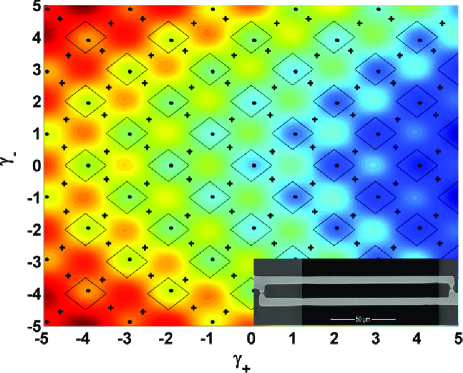
Figure 3: (Color online) Potential diagram of a DC SQUID, $u\left(\gamma_{+},\gamma_{-}\right)\,$, drawn using $I_{\mathrm{x}}=0.1I_{\mathrm{c}}$, and $\Phi_{\mathrm{x}}=0$. Local minima points are labeled by black dots and saddle points are labeled by plus signs. The inset shows a SEM image of a DC-SQUID.

Figure 3 plots the potential diagram of a DC-SQUID, calculated for E42 using $\beta_{\mathrm{L}}=83$ and $\alpha=0.032$. The solution of Eq. (5) produces the black closed curves that enclose the DC-SQUID local minima points in the plane of $\gamma_{+}$ and $\gamma_{-}$. The local minima points are labeled by black dots and saddle points are labeled by plus signs. A local minimum point losses its stability when increasing either $\left|I_{\mathrm{x}}\right|$ or $\left|\Phi_{\mathrm{x}}\right|$ to a point where it merges with one of the saddle points close to it.

The limits of small and large $\beta_{\mathrm{L}}$

In general, solving Eqs. (2) and (3) for a given set of $\gamma_{+}$ and $\gamma_{-}$ can only be done numerically. Analytical solution can be derived only for the extreme limits of $\beta_{\mathrm{L}}\ll 1$ and $\beta_{\mathrm{L}}\gg 1$. In the former limit, which is not the focus of this paper, the derivation leads to the well known formula for the SQUID critical current Clarke and Braginski (2004)

$$\sqrt{1-\left(1-\alpha^{2}\right)\sin^{2}\frac{\pi\Phi_{\mathrm{x}}}{\Phi_{0}}}=\frac{I_{\mathrm{x}}}{I_{\mathrm{c}}}.$$ (6)

In the opposite limit of $\beta_{\mathrm{L}}\gg 1$, the condition of $\det J=0$ implies that $\cos\gamma_{1}\cos\gamma_{2}=0$, and the condition of $\operatorname{tr}J>0$ implies that $\left(1+\alpha\right)\cos\gamma_{1}+\left(1-\alpha\right)\cos\gamma_{2}>0$. Consider first the solution for the minimum point near $\left(\gamma_{+},\gamma_{-}\right)=\left(0,0\right)$. Other solutions can be obtained from the periodic properties of Eqs. (2) and (3). For this solution, Eq. 5 is satisfied along a square that is formed by the lines connecting the four vertexes $\gamma_{1}=\pm\pi/2$ and $\gamma_{2}=\pm\pi/2$. Substituting these vertexes into Eqs. (2) and (3) yields a bounding contour which has a rectangle shape with vertexes at $\left(I_{\mathrm{x}}/I_{\mathrm{c}},~{}2\pi\Phi_{\mathrm{x}}/\Phi_{0}\beta_{\mathrm{L}}\right)=\left(1,\alpha\right)$, $\left(\alpha,1\right)$, $\left(-1,-\alpha\right)$ and $\left(-\alpha,-1\right)$ in the plane of the control parameters $I_{\mathrm{x}}$ and $\Phi_{\mathrm{x}}$ (see Fig. 4$\mathrm{(a)}$). This rectangle crosses the axis $I_{\mathrm{x}}=0$ at the points $\Phi_{\mathrm{x}}=\pm\Phi_{0}\beta_{\mathrm{L}}\left(1-\alpha\right)/2\pi$ and the axis $\Phi_{\mathrm{x}}=0$ at the points $I_{\mathrm{x}}=\pm I_{\mathrm{c}}\left(1-\alpha\right)$.

III.2 Equations of motion

Applying Kirchhoff’s laws on the DC-SQUID circuit model, substituting Josephson’s current-phase and voltage-phase equations, and taking into account the fluctuation dissipation theory, yields the following EOMs for the SQUID phases $\gamma_{1}$ and $\gamma_{2}$ Clarke and Braginski (2004)

$$\ddot{\gamma}_{1}+\beta_{\mathrm{D}}\dot{\gamma}_{1}+\left(1+\alpha_{0}\right)y\left(\Theta_{1}\right)\sin\gamma_{1}$$

$$+\frac{1}{\beta_{\mathrm{L0}}}\left(\gamma_{1}-\gamma_{2}+2\pi\Phi_{\mathrm{x}}/\Phi_{0}\right)=I_{\mathrm{x}}/I_{\mathrm{c}0}+g_{\mathrm{n}1},$$ (7)

$$\ddot{\gamma}_{2}+\beta_{\mathrm{D}}\dot{\gamma}_{2}+\left(1-\alpha_{0}\right)y\left(\Theta_{2}\right)\sin\gamma_{2}$$

$$-\frac{1}{\beta_{\mathrm{L0}}}\left(\gamma_{1}-\gamma_{2}+2\pi\Phi_{\mathrm{x}}/\Phi_{0}\right)=I_{\mathrm{x}}/I_{\mathrm{c}0}+g_{\mathrm{n}2},$$ (8)

where the overdot denotes a derivative with respect to a normalized time parameter $\tau=\omega_{\mathrm{pl}}t$, where $\omega_{\mathrm{pl}}$ is the SQUID plasma frequency, and $\beta_{\mathrm{D}}=1/\left(R_{\mathrm{J}}C_{\mathrm{J}}\omega_{\mathrm{pl}}\right)$ is the damping coefficient. In general, the NBJJ critical current, $I_{\mathrm{c}k}$ $(k=1,2)$, and thus $I_{\mathrm{c}}$ and $I_{\mathrm{c-}}$, are temperature dependant, as we discuss later. Thus we employ the notation $I_{\mathrm{c0}k}$, $I_{\mathrm{c0}}$, and $I_{\mathrm{c0-}}$ for the corresponding critical currents at a base temperature $T_{0}$, which is the temperature of the coolant. In addition, we employ the notation $\beta_{\mathrm{L0}}=\pi LI_{\mathrm{c0}}/\Phi_{0}$ and $\alpha_{0}=\left(I_{\mathrm{c0}1}+I_{\mathrm{c0}2}\right)/\left(I_{\mathrm{c0}1}-I_{\mathrm{c0}2}\right)$. The term $y\left(\Theta_{k}\right)$, where $\Theta_{k}=T_{k}/T_{\mathrm{c}}$ is the normalized temperature of the $k^{\mathrm{th}}$ NBJJ, expresses the dependence of the NBJJ critical current on its temperature, and is equal to unity as long as the temperature of the NBJJs are held at base temperature. The factor $g_{\mathrm{n}k}$ is a noise term, whose spectral density for the case where $h\nu/k_{\mathrm{B}}T\ll 1$ is given by $S_{I_{\mathrm{n}}}\left(\nu\right)=4k_{\mathrm{B}}T/R_{\mathrm{J}}$, with $k_{\mathrm{B}}$ being the Boltzmann constant. In what follows we neglect this noise term in the numerical simulations.

To evaluate the voltage across the DC-SQUID, denoted as $V_{\mathrm{SQD}}$, we assume that the loop inductance is equally divided between its two arms, and get

$$V_{\mathrm{SQD}}=\frac{1}{2}\left[\frac{\Phi_{0}}{2\pi}\left(\frac{\mathrm{d}\gamma_{1}}{\mathrm{d}t}+\frac{\mathrm{d}\gamma_{2}}{\mathrm{d}t}\right)+\frac{L}{2}\frac{\mathrm{d}I_{\mathrm{x}}}{\mathrm{d}t}\right].$$ (9)

It is known that NBJJs may have complex CPR Beenakker and VanHouten (1991); Golubov et al. (2004); Troeman et al. (2008), which deviates from the normal sinusoidal CPR of a regular JJ. According to a theory, brought in the appendix for completeness, such deviation would modify the $\sin\gamma_{i}$ term in the SQUID EOMs, Eqs. (7) and (8), which become Eqs. (25) and (26). We have made some simulations in which moderate changes in the CPR of our SQUIDs is assumed, and found no significant difference between these results and results that neglect this deviation. In addition, the physical dimensions of our NBJJs are relatively small, and the measured values of $\beta_{\mathrm{L}}$ of our SQUIDs are relatively high, thus following the explanations detailed in appendix $\mathrm{A1}$ of Ref. Suchoi et al. (2010), the effect of non-sinusoidal CPR in our NBJJs is expected to be negligibly small. Therefore, our conclusion is that our SQUIDs can be modeled by normal sinusoidal CPR.

III.3 Stability Diagram

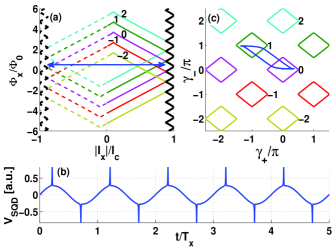
Figure 4: (Color online) $\mathrm{(a)}$ Stability diagram in the plane of the control parameters $I_{\mathrm{x}}$ and $\Phi_{\mathrm{x}}$, drawn for $\beta_{L}=20$ and $\alpha=0.1$. The curves are drawn using solid line for $I_{\mathrm{x}}>0$ and dashed line for $I_{\mathrm{x}}<0$. The number close to each curve labels the number of flux quanta trapped in the DC-SQUID in the corresponding LSZ. Corresponding numbers are also indicated in panel $\mathrm{(c)}$. The bold black curve marks the threshold between static and oscillatory zones. The double-headed blue arrow is drawn between the points $I_{\mathrm{x}}=\pm 0.9I_{\mathrm{c}}$, $\Phi_{\mathrm{x}}=0.52\Phi_{0}$, and marks the control parameter range used in the numerical simulation shown in panels $\mathrm{(b)}$ and $\mathrm{(c)}$. These panels show SQUID voltage in the time domain $\mathrm{(b)}$ and the NBJJs phases in the phase space $\mathrm{(c)}$. The time scale is normalized by the period of excitation $T_{\mathrm{x}}=\omega_{\mathrm{x}}/2\pi$.

The stability diagrams in the plane of the control parameters $I_{\mathrm{x}}$ and $\Phi_{\mathrm{x}}$, and in the plane of the DC-SQUID phases $\gamma_{+}$ and $\gamma_{-}$, are plotted in Fig. 4$\mathrm{(a)}$ and 4$\mathrm{(c)}$, respectively. The curves were first calculated in the plane of $\gamma_{+}$ and $\gamma_{-}$ by numerically solving Eq. (5), with the parameters $\beta_{\mathrm{L}}=20$ and $\alpha=0.1$. The above solutions were then substituted into Eqs. (2) and (3) to produce the closed contours of panel $\mathrm{(a).}$ Each closed contour bounds a Local Stability Zone (LSZ) corresponding to a different integer number of flux quanta trapped in the DC-SQUID. Corresponding LSZs in Fig. 4 $\mathrm{(a)}$ and 4$\mathrm{(c)}$ are labeled by the same number, indicating the number of trapped flux quanta.

The stability diagram can be separated into two global zones. The first is called static zone Inchiosa et al. (1999); Wiesenfeld et al. (2000), where the system has one or more LSZs depending of the value of the hysteresis parameter $\beta_{\mathrm{L}}$. The static zone is bounded in the horizontal axis by a threshold current called the oscillatory threshold, given by $I_{\mathrm{th}}\left(\Phi_{\mathrm{x}}\right)=I_{\mathrm{c}}-I_{-}\left(\Phi_{\mathrm{x}}\right)$. This threshold is periodic on the external flux $\Phi_{\mathrm{x}}$, having a maximum value equal to the critical current of the DC-SQUID. When the DC-SQUID is biased to the static zone, it is always found in a LSZ, though transitions between LSZs may be forced by the control parameters. The second zone, called oscillatory zone Inchiosa et al. (1999); Wiesenfeld et al. (2000) (also known as dissipative or free-running zone), spreads over two unbounded areas for which the excitation current is larger (in absolute value) than the oscillatory threshold. In this zone the DC-SQUID has no stable state; it oscillates at very high frequencies and dissipates energy. In what follows we focus our study on the static zone. Further study of the dynamics in the region of spontaneous oscillations can be found in Ref. Wiesenfeld et al. (2000).

III.4 SQUID Dynamics

The EOMs, Eqs. (7) and (8), were numerically integrated using the parameters which used to draw the stability diagram of Fig. 4, and using the control parameters $\Phi_{\mathrm{x}}=0.52\Phi_{0}$ and $I_{\mathrm{x}}/I_{\mathrm{c}}=0.9$. The range of the excitation is marked by a double-headed, blue arrow in the stability diagram of Fig. 4$\mathrm{(a)}$. Note that the left arrow head crosses the threshold separating LSZ_0 and LSZ_1 (LSZs corresponding to $0$ or $1$ trapped flux quanta, respectively); whereas the right headed arrow crosses the threshold separating LSZ_1 back into LSZ_0. The results of a simulation in which a DC-SQUID is periodically excited along this path are shown in Fig. 4. Panel $\mathrm{(b)}$ shows the DC-SQUID voltage in the time domain. Each excitation cycle contains two spikes, which occur close to extrema points of the excitation amplitude. Panel $\mathrm{(c)}$ shows the simulation in the phase plane of $\gamma_{+}$ and $\gamma_{-}$. The simulation shows that the system periodically switches between LSZ_0 and LSZ_1, and that the dynamics does not involve any additional LSZs. Thus a positive spike in the time-domain response corresponds to a transition from LSZ_0 to LSZ_1, and a negative spike corresponds to an opposite transition. When the excitation is monotonically increased the system mostly lingers in LSZ_0 and when it is decreased it mostly lingers in LSZ_1. Note that a serial resistor $R=0.5\operatorname{\Omega}$ was post-simulation added to the voltage results in order to emphasize the excitation cycle. Such a serial resistance also unavoidably exists in the wiring of our experimental setup. Note also that the duration of each spike, which is related to the relaxation time of the SQUID, is negligible compared to the period of excitation, $T_{\mathrm{x}}=\omega_{\mathrm{x}}/2\pi$. Thus, the assumption that the response of the DC-SQUID to the excitation is adiabatic is reasonable.

III.5 Periodic dissipative static zone

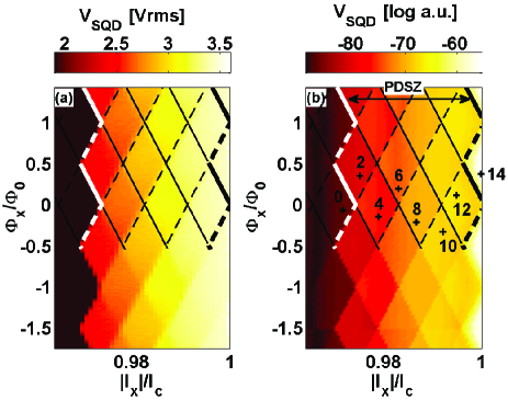
Figure 5: (Color online) Experimental $\mathrm{(a)}$ and numerical calculations $\mathrm{(b)}$ of direct voltage measurements and calculations of E38, in the parameter plane of $I_{\mathrm{x}}$ and $\Phi_{\mathrm{x}}$. Black contours mark the corresponding stability diagram, drawn using solid line for $I_{\mathrm{x}}>0$ and dashed line for $I_{\mathrm{x}}<0$. The diagram is applied only on half of the colormap in order to leave some data uncovered. The white bold contour marks the PDSZ threshold. Black bold contour marks the oscillatory threshold. Each plus sign marks a set of control parameters, and the corresponding number counts the LSZs boundaries that the SQUID periodically crosses if excited by that set of parameters.

Figure 5 shows a quantitative comparison between experimental results measured with E38 using lock-in amplifier (panel $\mathrm{(a)}$) and simulation results calculated using the corresponding parameters (panel $\mathrm{(b)}$). Both panels show colormaps of the voltage across the DC-SQUID as a function of control parameters, $I_{\mathrm{x}}$, and $\Phi_{\mathrm{x}}$. The black contours in both graphs mark the corresponding stability diagram. The negative part of the stability contours is folded onto the positive part and is drawn by dashed lines. Thus, solid lines represent stability thresholds for positive excitation currents, and dashed lines represent stability thresholds for negative excitation currents. The bold black contour is the threshold between the static zone and the oscillatory one.

The folding of the stability contours divides the static zone of the stability diagram into regions having diamond shapes in the plane of $I_{\mathrm{x}}$ and $\Phi_{\mathrm{x}}$. Each diamond region bounds a range of parameters for which the system crosses the same number of stability thresholds during an excitation cycle. For example, when excited with parameters bounded by the diamond marked by $2$, the DC-SQUID would cross a single threshold during the positive duration of the excitation cycle and another one during the negative duration, thus returning to the original LSZ, similar to the case discussed in Fig. 4$\mathrm{(c)}$. Each crossing of a threshold line, either by positive or negative currents, triggers a spike, which in turn contributes additively to the measured voltage across the DC-SQUID. Thus, each diamond bounds a range of parameters for which a similar voltage is measured. The diamonds follow the periodicity properties dictated for the control parameters by Eqs. (2) and (3).

We define an additional threshold, marked by bold white contour, which separates the static zone into two sections. In the first, which applies for periodic excitation currents smaller (in absolute value) than this threshold, the DC-SQUID is captured in a single LSZ after finite number of excitation cycles, and no spikes in the voltage appear afterwards. We call this section Periodic Non-Dissipative Static Zone (PNDSZ). In the second section, which spreads for excitation currents larger than the white threshold but smaller than the oscillatory threshold, the SQUID periodically jumps between LSZs and dissipates energy. Thus, we call this section Periodic Dissipative Static Zone (PDSZ), and call the white threshold itself the PDSZ threshold.

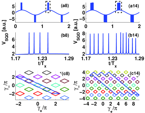
Figure 6: (Color online) Simulation results for E38. Panels $\mathrm{(a}i\mathrm{)}$, where $i=8,14$ corresponding to the marked points in Fig. 5, plot the DC-SQUID voltage in the time domain. panels $\mathrm{(b}i\mathrm{)}$ magnify the corresponding marked squares in panels $\mathrm{(a}i\mathrm{)}$. Panels $\mathrm{(c}i\mathrm{)}$ show the simulation results and the corresponding stability zones in the phase space of $\gamma_{+}$ and $\gamma_{-}$.

$$\begin{array}[c]{cc}\text{{\includegraphics[height=197.28246pt,width=241.67816pt]{Fig7a.eps}} }&\text{{\includegraphics[height=194.2179pt,width=241.67816pt]{Fig7b.eps}} }\end{array}$$

Figure 7: (Color online) Experimental measurements obtained from E42. Panels $\mathrm{(a)}$ and $\mathrm{(d)}$ draw the first and second SQUID voltage harmonics respectively. Panel $\mathrm{(b)}$ draws the voltage noise level at frequency of 1kHz. Panel $\mathrm{(c)}$ draws a statistical analysis of time-domain voltage traces, which calculates the difference between probabilities of measuring positive and negative voltage spikes respectively.

Figure 6 shows results of two simulations, calculated using the control parameters marked by points $8$ and $14$ in Fig. 5. Panels $\mathrm{(a}i\mathrm{)}$ where $i=8,14$ show the DC-SQUID voltage as a function of time, calculated during two excitation cycles. Each cycle has a bunch of spikes during its positive duration and another bunch during the negative one. Panels $\mathrm{(b}i\mathrm{)}$ magnify the corresponding bunch of spikes marked by dashed squares in panels $\mathrm{(a}i\mathrm{)}$. In panel $\mathrm{(b8)}$ one counts four spikes corresponding to four crossings of stability thresholds. Panel $\mathrm{(c8)}$ shows the phase space dynamics in the plane of $\gamma_{-}$ and $\gamma_{+}$. The system periodically cycles between five LSZs, where most of the time it lingers either in the upper left or in the lower right LSZs. The transition between these LSZs is forced by the driving sinusoidal bias current, which induces four jumps, corresponding to the four spikes in panel $\mathrm{(b8)}$. Panels $\mathrm{(b14)}$ and $\mathrm{(c14)}$ show a richer dynamics, which emerges from the fact that point $\mathrm{+14}$ is located inside the oscillatory zone. The dynamics includes both forced transitions between LSZs and spontaneous oscillations related to the oscillatory zone. These two kinds of transitions are clearly seen in Fig. 5, panel $\mathrm{(c14)}$, which plots the dynamics of $\gamma_{+}$ and $\gamma_{-}$ in the phase space. The first kind, in which $\gamma_{-}$ and $\gamma_{+}$ change monotonically, corresponds to forced transitions between LSZs. The second kind, in which the system cranks between LSZs, corresponds to the spontaneous oscillatory dynamics. The spontaneous oscillations last as long as the temporal driving bias current is greater than the oscillatory threshold. The distinction between the forced transitions and the spontaneous oscillations can also be noticed in the time domain, shown in Fig. 5, panel $\mathrm{(b14)}$, where the first six spikes are similar and distinct, whereas the rest of the spikes emerge in pairs, in which one spike is slightly stronger than the other.

III.6 Hybrid Oscillatory Zones

Figure 7 shows low-frequency experimental measurements of E42 DC-SQUID, which has a moderated self-inductance parameter $\beta_{\mathrm{L}}=83$ (compared to the one of E38). Similar to the experiment with E38, we excite the SQUID by a sinusoidal current having frequency of $\omega_{\mathrm{x}}/2\pi=2.5\operatorname{kHz}$, and measure the voltage across the DC-SQUID as a function of excitation current $I_{\mathrm{x}}$ and external magnetic flux $\Phi_{\mathrm{x}}$. In addition, we measure the spectral density of the voltage using a spectrum analyzer and its response in the time domain using an oscilloscope. Figure 7$\mathrm{(a)}$ shows this voltage and has the corresponding folded stability diagram drawn on it. The colormap, which focuses on the oscillatory threshold, reveals an interesting phenomenon. The threshold related to positive excitation currents (solid bold line) is shifted compared to the one related to negative excitation currents (dashed bold line). This mismatch between the thresholds creates hybrid oscillatory zones, in which the DC-SQUID is driven to the oscillatory zone either for positive currents or negative currents, but not for both.

Figure 7$\mathrm{(b)}$ plots a colormap of the voltage noise level, measured using the spectrum analyzer at a frequency of $1\operatorname{kHz}$ (any frequency which is not an integer harmonics of $\omega_{\mathrm{x}}$ gives similar results). Plotting the noise level is a good way to detect thresholds since noise-rise is generally expected near any bifurcation threshold Huberman et al. (1980). Two distinct patterns of noise-rise are clearly seen in the colormap. One is related to the solid line positive threshold and the other to the dashed line negative threshold. Note that this noise-rise is almost undetectable in the lock-in measurements.

The existence of hybrid zones is easily observed in time domain measurements. Figure 8 shows two pairs of time domain traces, each pair has an experimental trace (panels $(\mathrm{1e})$, $(\mathrm{2e})$) and a simulated trace (panels $(\mathrm{1s})$, $(\mathrm{2s})$), measured (calculated) for the parameters labeled by plus marks and the corresponding number in Fig. 7$\mathrm{(a)}$ and 7$\mathrm{(b)}$. The first (second) pair is related to the hybrid zone where only positive (negative) currents drive the system to the oscillatory zone. Accordingly, the first (second) pair experiences only positive (negative) spikes. The difference between the measured and simulated line shapes of the spikes might be due to finite (about $\operatorname{MHz}$) bandwidth of our measurement setup which is far too low to resolve high frequency spikes. Therefore, measured spikes in the output signal merge into one continuous and slowly decaying pulse. Local heating effects, which are neglected in this simulation and will be discussed later, may also degrade DC-SQUID performance and suppress the spikes.

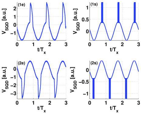
Figure 8: Time domain experimental measurements (left column) and numerical simulation (right column) for E42. The two rows correspond to the two sets of control parameters marked in Fig. 7.

A statistical analysis of the time-domain behavior is seen in Fig. 7$\mathrm{(c)}$, which plots the probability of counting a positive spike $P_{\mathrm{s}}^{\mathrm{pos}}$, minus the probability of counting a negative one $P_{\mathrm{s}}^{\mathrm{neg}}$, during a single lock-in excitation cycle. The probabilities were measured for the parameter range spanned by $I_{\mathrm{x}}$ and $\Phi_{\mathrm{x}}$, and were calculated on $2\sec$ long traces with $\omega_{\mathrm{x}}/2\pi=2.5\operatorname{kHz}$. This colormap clearly reveals the existence of the hybrid oscillatory zones, where the differential probability of counting spike having either positive or negative polarities is almost one. The direction of the spikes agrees with the prediction of the stability diagram. Outside the hybrid zones the colormap shows near zero differential probability. In these areas there are no spikes at all, or the counting of positive and negative spikes is similar. This behavior could be used for creating bidirectional DC-SQUID sensors in which the polarity of measured voltage indicates the polarity of the detected flux change. Panel $\mathrm{(d)}$ plots the second harmonics of the measured SQUID voltage (at $5\operatorname{kHz}$). This harmonics is expected to be amplified when the measured voltage is asymmetric in time, i.e. neither symmetric nor anti-symmetric time response. The hybrid zones are characterized by such a time response, and indeed, the plotted colormap shows strong response of the second harmonics in those zones.

IV Parametric Excitation

In recent years several demonstrations of using SQUIDs to manipulate the resonance frequencies of a superconducting resonator were reported Suchoi et al. (2010); Sandberg et al. (2008); Castellanos-Beltran and Lehnert (2007); Palacios-Laloy et al. (2008). A SQUID in such applications is usually considered as a nonlinear variable inductor embedded in the resonator in a way that couples the resonance frequencies of the resonator to the SQUID impedance. The variation of the SQUID inductance is usually done by changing the magnetic flux through the SQUID, whereas the current through the SQUID is defined by the state of the coupled system.

IV.1 Stability Zones

In the following, we analyze the stability of a DC-SQUID, excited by a magnetic flux having constant and alternating parts. Consider the case where $\Phi_{\mathrm{x}}$ is given by

$$\Phi_{\mathrm{x}}=\Phi_{0}\left(\Phi_{\mathrm{x}}^{\mathrm{dc}}+\Phi_{\mathrm{x}}^{\mathrm{ac}}\cos\left(\omega_{\mathrm{px}}t\right)\right),$$ (10)

where $\Phi_{\mathrm{x}}^{\mathrm{dc}}/\Phi_{0}$ and $\Phi_{\mathrm{x}}^{\mathrm{ac}}/\Phi_{0}$ are arbitrary amplitudes. Recall that for the case of $\beta_{\mathrm{L}}\gg 1$, and for the minimum point near $\left(\gamma_{+},\gamma_{-}\right)=\left(0,0\right)$, the bounding rectangle crosses the axis $I_{\mathrm{x}}=0$ at the points $\Phi_{\mathrm{x}}=\pm\Phi_{0}\widetilde{\beta}_{\mathrm{L}}/2\pi$, where $\widetilde{\beta}_{\mathrm{L}}=\left(1-\alpha\right)\beta_{\mathrm{L}}$. The range of stability for the minima points near $\left(\gamma_{+},\gamma_{-}\right)=\left(n\pi,n\pi\right)$, where $n$ is integer, is given by

$$-\frac{\widetilde{\beta}_{\mathrm{L}}}{2\pi}+n\leq\frac{\Phi_{\mathrm{x}}}{\Phi_{0}}\leq\frac{\widetilde{\beta}_{\mathrm{L}}}{2\pi}+n.$$ (11)

Furthermore, the stability condition is achieved when the largest value of $\Phi_{\mathrm{x}}$, i.e. $\Phi_{\mathrm{x}}^{\mathrm{dc}}+\Phi_{\mathrm{x}}^{\mathrm{ac}}$, coincides with the largest value of the stability range, i.e. $\widetilde{\beta}_{\mathrm{L}}/2\pi$, or when the smallest value of $\Phi_{\mathrm{x}}$, i.e. $\Phi_{\mathrm{x}}^{\mathrm{dc}}-\Phi_{\mathrm{x}}^{\mathrm{ac}}$, coincides with the smallest value of the stability range, i.e. $-\widetilde{\beta}_{\mathrm{L}}/2\pi$. Thus the boundary contours in the plan of $\Phi_{\mathrm{x}}^{\mathrm{dc}}$ and $\Phi_{\mathrm{x}}^{\mathrm{ac}}$ are given by the two equations

$$\Phi_{\mathrm{x}}^{\mathrm{dc}}\pm\Phi_{\mathrm{x}}^{\mathrm{ac}}=\pm\Phi_{0}\frac{\widetilde{\beta}_{\mathrm{L}}}{2\pi}+n\Phi_{0}.$$ (12)

In experiments with resonators we employ the parametric amplification method of operation Castellanos-Beltran et al. (2008, 2009); Thol n et al. (2009); Yamamoto et al. (2008). We inject a relatively weak probing signal into the resonator, having frequency equals to one of the resonance frequencies of the resonator, $\omega_{\mathrm{x}}$, and measure the reflected power off the resonator using a spectrum analyzer. Note that the DC connections do not play any role in this measurement. A weak signal is a one for which the current generated through the SQUID is much smaller than its critical current. In addition, we applied constant and variable magnetic flux through the SQUID, given by Eq. (10) with $\omega_{\mathrm{px}}=\left(2\omega_{\mathrm{x}}+\Delta\omega\right)$, where $\Delta\omega$ is taken to be much smaller than the resonance bandwidth of the resonator. The measured reflected power spectrum includes a tone at $\omega_{\mathrm{x}}$ and several sidebands spaced by $\pm m\cdot\Delta\omega$ from $\omega_{\mathrm{x}}$, where $m$ is an integer. These sidebands are the products of the nonlinear frequency mixing between $\omega_{\mathrm{x}}$ and $\omega_{\mathrm{px}}$. Although this mixing process is more complex than our direct SQUID measurements, it should essentially follow the same SQUID dynamics, provided that adiabatic approximation is not violated, namely $\omega_{\mathrm{x}}\ll\omega_{\mathrm{pl}}$. Therefore, we expect the various tones to reflect that dynamics.

Figure 10$\mathrm{(a)}$ shows the folded stability diagram, drawn in the plane of $\Phi_{\mathrm{x}}^{\mathrm{dc}}$ and $\Phi_{\mathrm{x}}^{\mathrm{ac}}$ using Eq. (12) and $\widetilde{\beta}_{\mathrm{L}}=45$. The solid and dashed lines represent stability thresholds for positive and negative polarities of $\Phi_{\mathrm{x}}^{\mathrm{ac}}$, respectively. Four pairs of solid-dashed lines are drawn, each corresponds to a different number of flux quanta trapped in the SQUID. The black bold line marks the threshold between the PNDSZ and the PDSZ. Namely, for excitation amplitudes $\left|\Phi_{\mathrm{x}}^{\mathrm{ac}}\right|$ smaller than the black line, the SQUID will reach a LSZ after a finite number of excitation periods. On the other hand for $\left|\Phi_{\mathrm{x}}^{\mathrm{ac}}\right|$ higher than the black line the SQUID will periodically jump between LSZs. Note that in this method of excitation, where the injected current is kept much smaller than the critical current, the SQUID would not be driven to the oscillatory zone, even by an arbitrarily large $\Phi_{\mathrm{x}}^{\mathrm{ac}}$.

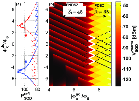
Figure 9: (Color online) Parametric excitation experimental $\mathrm{(a)}$ and simulation $\mathrm{(b)}$ results. $\mathrm{(a)}$ Reflected power of the second voltage harmonics as a function of increasing (blue) and decreasing (red) DC flux. $\mathrm{(b)}$ Simulated second voltage harmonics in the plane of $\Phi_{\mathrm{x}}^{\mathrm{ac}}$ and $\Phi_{\mathrm{x}}^{\mathrm{dc}}$. The black contours mark the corresponding stability diagram drawn for $\widetilde{\beta}_{\mathrm{L}}=45$. White bold contours mark the threshold to the PDSZ.

Figure 9$\mathrm{(b)}$ shows the simulated second voltage harmonics across the SQUID, i.e. at frequency $\omega=2\omega_{\mathrm{px}}$, and for $\Delta\omega=0$, obtained using E42 parameters. The black contours, which are similar to the ones in Fig. 10$\mathrm{(a)}$, mark the stability diagram. The distinction between the periodic non-dissipative and periodic dissipative static zones is clear, and is marked by the white bold PDSZ threshold. Like before with the SQUID of E38, the PDSZ is characterized by relatively high SQUID voltage, which is divided into diamond shaped regions. The PNDSZ, unlike with E38, is also characterized by strong response along the stability contours. When one such contour is crossed, a single transition between LSZ occurs. After this transition no additional transitions would periodically occur. Nevertheless, these boundaries are detectable due to the fact that the inductance of the SQUID before and after a transition is different, and also due to the fact that the excitation frequency is high, thus the effect of changes in the SQUID inductance is measurable. Only transitions across the solid stability contours are observed in the colormap of Fig. 9. The reason is the sequence of the measurement, which includes sweeping the DC flux monotonically up and down in the inner simulation loop. The colormap is obtained while the flux amplitude is increased, thus transitions over the solid contours are recorded; whereas the decreasing section is only used to maintain the consecutiveness of initial condition, similar to the experiments.

Figure 9$\mathrm{(a)}$ shows measurement results obtained from E42. A probe tone having frequency of $\omega_{\mathrm{x}}$ is injected into the resonator, and the reflected power of the second order sideband, i.e. the tone at $\omega_{\mathrm{x}}+\Delta\omega$, is measured, while the DC flux is swept up (blue curve, marked by up headed arrow) and down (red curve, marked by down headed arrow), and while keeping the AC flux at a fixed amplitude. Following the blue curve from bottom to top, the reflected power experiences a resonance-like absorption followed by a saw teeth pattern. The resonance absorption pattern originates from the tuning of the resonance frequency of the resonator relatively to the frequency of the probing signal, thus effectively sweeping the probe in and out of resonance. This sweeping is caused by the SQUID, which has flux dependent inductance Suchoi et al. (2010), even when stuck in a single LSZ. After the SQUID is driven across a stability threshold it falls to a new LSZ, into a location which is one flux quantum away from the corresponding stability contour. Thus, if the external flux is further increased, it would further drives the SQUID to the same direction, and additional transitions would occur, spaced apart by one flux quantum. If, on the other hand, the direction of the sweep changes (red curve), the SQUID would first have to be driven across a whole LSZ, until reaching the opposite stability threshold. Therefore, no matter where the flux sweep changes direction along the saw teeth pattern, the reflected power would experiences a resonance-like absorption followed by saw teeth pattern.

Looking back at Fig. 9$\mathrm{(b)}$, the sweeping of $\Phi_{\mathrm{x}}^{\mathrm{dc}}$ up and down usually drives back the SQUID to its original LSZ. When the AC flux amplitude $\Phi_{\mathrm{x}}^{\mathrm{ac}}$ is increased, the borders of a LSZ enclose one another. As a result, the sweep across the first stability zone becomes shorter, and hence the resonance absorption pattern becomes narrower along the DC flux axis. This narrowing adds saw teeth along the sweep range, and in addition, the SQUID might no longer return to its original LSZ, but rather to a new LSZ, which correspond to a change of one in the number of trapped flux quanta. This creates the sharp transition observed in the resonance-like absorption patterns along the horizontal axis.

IV.2 Temperature dependant critical current

When a SQUID is embedded in a resonator, the current $I_{\mathrm{x}}$ flowing through the SQUID is driven by the resonator, and its frequency, thus equals to one of the resonance frequencies of the resonator. These first few frequencies are only about two to three orders of magnitude lower than the plasma frequency of the SQUID Suchoi et al. (2010). Furthermore, the heat transfer rate corresponding to hot-spots in the NBJJs may be of the order as those frequencies or even slower Tarkhov et al. (2008), and therefore effect of heating on the dynamics of the SQUID becomes significant. Assuming for simplicity that the temperature $T_{k}$ ($k=1,2$) in each junction is uniform. The dependence of the critical current on the temperature is given by Skocpol (1976)

$$\frac{I_{\mathrm{c}k}}{I_{\mathrm{c}0k}}=y\left(\Theta_{k}\right)\equiv\frac{\widetilde{y}\left(\Theta_{k}\right)}{\widetilde{y}\left(\Theta_{0}\right)},$$ (13)

where $I_{\mathrm{c}0k}$ is the critical current of $k^{\mathrm{th}}$ NBJJ at base temperature $T_{0}$ of the coolant, $\Theta_{k}=T_{k}/T_{\mathrm{c}}$ is normalized temperature of the NBJJ (with respect to its critical temperature), $\Theta_{0}=T_{0}/T_{\mathrm{c}}\,$, and where the function $\widetilde{y}$ is given by

$$\widetilde{y}\left(\Theta\right)=\left(1-\Theta^{2}\right)^{3/2}\left(1+\Theta^{2}\right)^{1/2}.$$ (14)

The $k^{\mathrm{th}}$ ($k=1,2$) NBJJ heat balance equations read

$$C_{k}\frac{\mathrm{d}T_{k}}{\mathrm{d}t}=Q_{k}-H_{k}\left(T_{k}-T_{0}\right),$$ (15)

where $C_{k}$ is thermal heat capacity, $Q_{k}=V_{k}^{2}/R_{\mathrm{J}}$ is heating power, and $H_{k}$ is heat transfer coefficient. By using the notation $\beta_{\mathrm{C}k}=2\pi C_{k}T_{\mathrm{c}}/\Phi_{0}I_{\mathrm{c}0}$ and $\beta_{\mathrm{H}k}=H_{k}C_{k}\omega_{\mathrm{p}}$, Eq. 15 becomes

$$\dot{\Theta}_{k}=\frac{\beta_{\mathrm{D}}}{\beta_{\mathrm{C}k}}\dot{\gamma}_{k}^{2}-\beta_{\mathrm{H}k}\left(\Theta_{k}-\Theta_{0}\right).$$ (16)

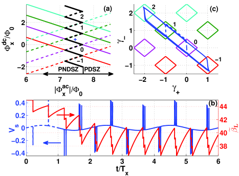
Figure 10: (Color online) $\mathrm{(a)}$ Stability zones in the plan of the control parameters $\Phi_{\mathrm{x}}^{\mathrm{ac}}$ and $\Phi_{\mathrm{x}}^{\mathrm{dc}}$, drawn for $\widetilde{\beta}_{L}=45$. The curves are drawn using solid lines for $\Phi_{\mathrm{x}}^{\mathrm{ac}}>0$ and dashed lines for $\Phi_{\mathrm{x}}^{\mathrm{ac}}<0$. The numbers beside each pair crossing represent the total magnetic flux quanta trapped in the SQUID in the corresponding LSZ (in units of $\Phi_{0}$). The bold black curve marks the PDSZ threshold. Simulation results of the SQUID voltage and $\widetilde{\beta}_{\mathrm{L}}$ in the normalized time domain $\mathrm{(b)}$, and $\gamma_{+}$ and $\gamma_{-}$ in the phase space $\mathrm{(c)}$. The simulation is calculated using the set of control parameters marked by the plus sign in panel $\mathrm{(a)}$. Time is normalized by the period of probing tone injected to the resonator, $T_{\mathrm{x}}$,

Figure 10, panels $\mathrm{(b)}$ and $\mathrm{(c),}$ show simulation results of the SQUID voltage and $\widetilde{\beta}_{\mathrm{L}}$ in the time domain $\mathrm{(b),}$ and $\gamma_{+}$ and $\gamma_{-}$ in the phase space $\mathrm{(c)}$, calculated for the control parameters marked by the plus sign in Fig. 10$\mathrm{(a)}$. The temperature in this simulation is not held at the base temperature but rather evolves according to Eq. (16). The parameters $\beta_{\mathrm{C}k}=$ $320$ and $\beta_{\mathrm{H}k}=$ $5\times 10^{-4}$ ($k=1,2$) were calculated analytically according to Refs. Johnson et al. (1996); Weiser et al. (1981); Monticone et al. (1999). Further explanations about parameters calculation is found in appendix $\mathrm{B}$ of Ref. Suchoi et al. (2010). One expects that for the chosen control parameters the SQUID would oscillates between two LSZs. The dynamics plotted in panel $\mathrm{(c)}$, however, shows that this is true only during the first excitation cycle (dashed line), and that afterwards the SQUID oscillates between four LSZs. Such a change in the dynamic behavior of the SQUID is also observed in the time domain voltage trace plotted in panel $\mathrm{(b)}$. The number of voltage spikes increases from one during the first excitation cycle (dashed line) to three in the end of the second excitation cycle (solid line). This behavior can be explained by the dynamical change in the value of $\widetilde{\beta}_{\mathrm{L}}$, plotted as red curve in panel $\mathrm{(b)}$. The hysteretic parameter $\widetilde{\beta}_{\mathrm{L}}$ experiences relaxation oscillations having their mean value changing during the first three excitation cycles. The relaxation oscillations are driven by the voltage spikes which dissipate energy and produce heat. This heat increases the temperature of the NBJJs, which in turn decreases their critical current according to Eq. (13), thus decreasing the value of $\beta_{\mathrm{L}}$. The reduction in $\beta_{\mathrm{L}}$ results in a shift of the stability diagram towards the origin, and consequently the given set of control parameters effectively drives the SQUID between increased numbers of LSZs.

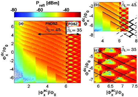
Figure 11: (Color online) Parametric excitation experimental results. The colormaps show the reflected power off the resonator in the plane of $\Phi_{\mathrm{x}}^{\mathrm{ac}}$ and $\Phi_{\mathrm{x}}^{\mathrm{dc}}$. Panels $\mathrm{(b)}$ and $\mathrm{(c)}$ show the fitting of the stability diagram to the measured data using $\widetilde{\beta}_{\mathrm{L}}=45$ and $\widetilde{\beta}_{\mathrm{L}}=35$, respectively.

Figure 11 shows the reflected power of the second order mixing product, i.e. the tone at $\omega_{\mathrm{x}}+\Delta\omega$, measured in the plane of $\Phi_{\mathrm{x}}^{\mathrm{dc}}$ and $\Phi_{\mathrm{x}}^{\mathrm{ac}}$ from E42. This measurement corresponds to the simulation shown in Fig. 9. The figure contains three panels, where panels $\mathrm{(b)}$ and $\mathrm{(c)}$ show partial sections of the main colormap shown in panel (a), each with a corresponding fit of the stability diagram. Looking at panel $\mathrm{(a)}$, most of the observations agree well with the simulated results, seen in Fig. 9. The PDSZ is characterized by strong reflection response and stability regions having diamond shapes. The PNDSZ experiences strong response along the boundaries of the LSZs. The response lines slightly bend for low excitation amplitudes ($\Phi_{\mathrm{x}}^{\mathrm{ac}}\lesssim 3\Phi_{0}$), but follow rather strait line for higher amplitudes. Good fitting of the stability diagram to these lines is achieved with $\widetilde{\beta}_{\mathrm{L}}=45$, as shown in panel $\mathrm{(b)}$. The bending of the boundary lines at low amplitudes might be due to slow rise of the average temperatures of the SQUID. The reason why only transitions across solid stability contours are measured is the measurement protocol, which includes a sweep of the DC flux up and down in the inner measurement loop, while measurements are recorded only during the incremental duration of the sweep. In addition to the emerging of the LSZ boundaries in the measurement, also the influence of the variation of the SQUID inductance within a LSZ on the reflected power is observed. Furthermore, the sharp transitions along the horizontal axis, corresponding to DC flux sweeps that do not drive the SQUID back to its original LSZ, are observed at $\Phi_{\mathrm{x}}^{\mathrm{ac}}/\Phi_{0}=[1.4,2.75,4.05,4.74]$, in agreement with the simulation results.

The stability diagram in Fig. 11$\mathrm{(b)}$, drawn for $\widetilde{\beta}_{\mathrm{L}}=45$, predicts that the PDSZ threshold should zigzag along the stability contours in the range of $\Phi_{\mathrm{x}}^{\mathrm{ac}}/\Phi_{0}\in[7.5,8]$. The measured colormap, however, shows that the PDSZ threshold passes along a strait vertical line starting at point $(\Phi_{\mathrm{x}}^{\mathrm{dc}}=-6.25\Phi_{0},\Phi_{\mathrm{x}}^{\mathrm{ac}}=5.95\Phi_{0})$. A fitting process of the stability diagram to the PDSZ section itself produces $\widetilde{\beta}_{\mathrm{L}}\mathbf{=}35$ (see Fig. 11$\mathrm{(c))}$. This duality in the value of $\beta_{\mathrm{L}}$ can be understood if changes of the SQUID temperature are taken into account. The PDSZ threshold point exactly coincides with one of the LSZ threshold contours. The heat generated in single transition across that threshold momentarily decreases $\widetilde{\beta}_{\mathrm{L}}$. An additional transition may be triggered provided that the relaxation of the first one lasts long enough, which in turn may cause further heating of the DC-SQUID. Eventually a new mean temperature is achieved for which $\widetilde{\beta}_{\mathrm{L}}=35$. The measurement protocol dictates that this new temperature would be kept and that the DC-SQUID would stay in the PDSZ for the rest of the measurement. Note that the initial value of $\widetilde{\beta}_{\mathrm{L}}=45$ differs from the value of $\widetilde{\beta}_{\mathrm{L}}=80$ that was measured using lock-in amplifier. This can be explained by the local heating that the high frequency flux excitation induces in the DC-SQUID, especially in the NBJJs, through the dissipation of circulating current due to RF surface resistance. Such reduction in $\widetilde{\beta}_{\mathrm{L}}$ from $80$ to $45$ may be induced by a change of the local temperature by approximately $2\operatorname{K}$.

IV.3 The Case of RF SQUID Parametric Excitation

The stability diagram for a DC-SQUID can be evaluated numerically, or be analytically approximated for the extreme cases of $\beta_{\mathrm{L}}\ll 1$ and $\beta_{\mathrm{L}}\gg 1$. For RF-SQUID, on the other hand, it could be exactly evaluated analytically. Consider a RF-SQUID having self-inductance $L$, critical current $I_{\mathrm{c}}$, and externally applied magnetic flux $\Phi_{\mathrm{x}}=\left(\Phi_{0}/2\pi\right)\phi_{\mathrm{x}}$. The dynamics of the total magnetic flux $\Phi=\left(\Phi_{0}/2\pi\right)\phi$ threading the RF-SQUID loop is governed by the potential energy $U=U_{0}u_{\mathrm{RF}}$ Buks and Blencowe (2006), where

$$u_{\mathrm{RF}}=\left(\phi-\phi_{\mathrm{x}}\right)^{2}-2\beta_{\mathrm{L}}\cos\phi,$$ (17)

and $U_{0}=\Phi_{0}^{2}/\left(8\pi^{2}L\right)$. A local minimum point of $u_{\mathrm{RF}}$ is found by solving $\partial u_{\mathrm{RF}}/$ $\partial\phi=0$ and requiring that $\partial^{2}u/\partial\phi^{2}>0$. Clearly, if $\phi_{\mathrm{m}}$ is a local minimum point of the potential $u_{\mathrm{RF}}$ with a given $\phi_{\mathrm{x}}$, then $\phi_{\mathrm{m}}+2n\pi$ is also a local minimum point of the potential $u_{\mathrm{RF}}$ with an externally applied flux of $\phi_{\mathrm{x}}+2n\pi$, provided that $n$ is integer.

Lose of stability occurs when $\partial^{2}u/\partial\phi^{2}=0$, namely when $\cos\phi=-1/\beta_{\mathrm{L}}$. This can occur only when $\beta_{\mathrm{L}}>1$, since otherwise the system is expected to be monostable. This condition is satisfied when $\phi_{\mathrm{x}}=\phi_{\mathrm{x,b}}$, where

$$\phi_{\mathrm{x,b}}=\pi-\arccos\left(\frac{1}{\beta_{\mathrm{L}}}\right)+\sqrt{\beta_{\mathrm{L}}^{2}-1}.$$ (18)

For a general integer $n$, the local minimum of the potential $u_{\mathrm{RF}}$ near $\phi=2n\pi$ remains stable in the range

$$-\phi_{\mathrm{x,b}}+2n\pi\leq\phi_{\mathrm{x}}\leq\phi_{\mathrm{x,b}}+2n\pi.$$ (19)

Similarly to the case of DC-SQUID, where $\Phi_{\mathrm{x}}$ is given by Eq. (10), the boundary contours in the plan of $\Phi_{\mathrm{x}}^{\mathrm{dc}}$ and $\Phi_{\mathrm{x}}^{\mathrm{ac}}$ are given by the two equations

$$\Phi_{\mathrm{x}}^{\mathrm{dc}}\pm\Phi_{\mathrm{x}}^{\mathrm{ac}}=\Phi_{0}\left(\pm\frac{\phi_{\mathrm{x,b}}}{2\pi}+n\right),$$ (20)

for the largest and smallest values of $\Phi_{\mathrm{x}}$, respectively.

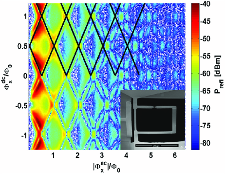
Figure 12: (Color online) Parametric excitation experimental results using E19, which has an integrated RF-SQUID. The colormap shows the reflected power off the resonator in the plane of $\Phi_{\mathrm{x}}^{\mathrm{ac}}$ and $\Phi_{\mathrm{x}}^{\mathrm{dc}}$. The black contours mark the corresponding stability diagram. They are applied only on half of the colormap in order to leave some data uncovered. The inset shows a SEM image of a RF SQUID.

Figure 12 shows the reflected power of the third order mixing product, i.e. the tone at $\omega_{\mathrm{x}}+2\Delta\omega$, measured in the plane of $\Phi_{\mathrm{x}}^{\mathrm{dc}}$ and $\Phi_{\mathrm{x}}^{\mathrm{ac}}$ with E19, which has an embedded RF-SQUID instead of a DC-SQUID. The black contours represent the stability diagram, plotted using Eqs. (20) for $\beta_{\mathrm{L}}=1.5$. The stability diagram qualitatively matches the measured data for the first few stability diamonds.

Note that the value of $\beta_{\mathrm{L}}$ for the RF-SQUID of E19 is more than order of magnitude smaller than that of E38 and E42. This might be due to the fact that this RF-SQUID is fully fabricated on Silicon Nitride membrane, and thus has reduced thermal coupling to the coolant compared to the DC-SQUIDs of E38 and  E42. This in turn might lead to an increased local temperature of the NBJJ, and to a degraded value of $\beta_{\mathrm{L}}$.

Note also that the diamonds themselves have distinct reflection patterns inside their bounded zone (see Figs. 11 and 12), which are not perfectly periodic with $\Phi_{\mathrm{x}}^{\mathrm{ac}}$, but are reproducible in measurements. They are only detected in measurements with resonators having either DC or RF SQUIDs, but not in measurements done directly with DC-SQUIDs. Our model only handles the DC-SQUID equations of motion, and thus cannot provide full description of the dynamics of the resonator-SQUID system. Further theoretical work is needed for modeling combined TLR-SQUID system, in order to fully understand these experimental results.

V Conclusions

In conclusion, we have studied the response of a nano-bridge based SQUID embedded in a superconducting microwave resonator. nano-bridge based SQUIDs are usually characterized by high critical current, and thus enhanced metastable and hysteretic response. Several phenomena were observed, including periodic dissipative static zone in which periodic transitions between local stable state occur; hybrid oscillatory zones, in which the SQUID is driven to the oscillatory zone by one polarity of the excitation amplitude but not for the other, and dynamical variations in $\beta_{\mathrm{L}}$ due to the effect of self-heating. The behaviors of the SQUIDs were compared with theory both analytically and numerically with good agreement.

E.S. is supported by the Adams Fellowship Program of the Israel Academy of Sciences and Humanities. This work is supported by the German Israel Foundation under grant 1-2038.1114.07, the Israel Science Foundation under grant 1380021, the Deborah Foundation, the Poznanski Foundation, Russell Berrie nanotechnology institute, Israeli Ministry of Science, the European STREP QNEMS project, and MAFAT.

Appendix A Nano-bridge current-phase relation

The CPR of a single short channel of transmission $\tau$ is given by Beenakker and VanHouten (1991)

$$I=\frac{e\Delta}{2\hbar}J\left(\gamma\right)\;,$$ (21)

where

$$J\left(\gamma\right)=\frac{\tau\sin\gamma}{\sqrt{1-\tau\sin^{2}\frac{\gamma}{2}}}\;.$$ (22)

The NBJJs in our devices are not ideal one dimensional point contacts as Ref. Beenakker and VanHouten (1991) assumes, however, we have found that the above simple analytical result resembles the CPR which is obtained by solving the Ginzburg-Landau equation in the limit of short bridge (in comparison with the coherence length) Likharev (1979). Let $\gamma_{0}$ be the point at which the factor $J\left(\gamma\right)$ has its largest value $J\left(\gamma_{0}\right)$, which is given by

$$J\left(\gamma_{0}\right)=2\sqrt{2\left(1-\sqrt{1-\tau}\right)-\tau}\;.$$ (23)

Using this result the current $I$ can be written in terms of $I_{\mathrm{c}}$ as $I/I_{\mathrm{c}}=F\left(\gamma\right)$, where

$$F\left(\gamma\right)=\frac{\tau\sin\gamma}{2\sqrt{2\left(1-\sqrt{1-\tau}\right)-\tau}\sqrt{1-\tau\sin^{2}\frac{\gamma}{2}}}\;.$$ (24)

Replacing the $\sin\gamma_{\mathrm{k}}$ terms ($k=1,2$) in Eqs. (7) and (8) by $F\left(\gamma_{\mathrm{k}}\right)$ leads to the following modified EOMs

$$\ddot{\gamma}_{1}+\beta_{\mathrm{D}}\dot{\gamma}_{1}+\left(1+\alpha_{0}\right)y\left(\Theta_{1}\right)F\left(\gamma_{1}\right)$$

$$+\frac{1}{\beta_{\mathrm{L0}}}\left(\gamma_{1}-\gamma_{2}+2\pi\Phi_{\mathrm{x}}/\Phi_{0}\right)=I_{\mathrm{x}}/I_{\mathrm{c}0}+g_{\mathrm{n}1},$$ (25)

and

$$\ddot{\gamma}_{2}+\beta_{\mathrm{D}}\dot{\gamma}_{2}+\left(1-\alpha_{0}\right)y\left(\Theta_{2}\right)F\left(\gamma_{2}\right)$$

$$-\frac{1}{\beta_{\mathrm{L0}}}\left(\gamma_{1}-\gamma_{2}+2\pi\Phi_{\mathrm{x}}/\Phi_{0}\right)=I/I_{\mathrm{c}0}+g_{\mathrm{n}2}.$$ (26)

References

- Chiorescu et al. (2004) I. Chiorescu, P. Bertet, K. Semba, Y. Nakamura, C. J. P. M. Harmans, and J. E. Mooij, Nature 431, 159 (2004).
- Johansson et al. (2006) J. Johansson, S. Saito, T. Meno, H. Nakano, M. Ueda, K. Semba, and H. Takayanagi, Phys. Rev. Lett. 96, 127006 (2006).
- Houck et al. (2007) A. A. Houck, D. I. Schuster, J. M. Gambetta, J. A. Schreier, B. R. Johnson, J. M. Chow, L. Frunzio, J. Majer, M. H. Devoret, S. M. Girvin, et al., Nature 449, 328 (2007).
- Majer et al. (2007) J. Majer, J. M. Chow, J. M. Gambetta, J. Koch, B. R. Johnson, J. A. Schreier, L. Frunzio, D. I. Schuster, A. A. Houck, A. Wallraff, et al., Nature 449, 443 (2007).
- Sillanpaa et al. (2007) M. A. Sillanpaa, J. I. Park, and R. W. Simmonds, Nature 449, 438 (2007).
- Astafiev et al. (2010a) O. Astafiev, A. M. Zagoskin, J. Abdumalikov, A. A., Y. A. Pashkin, T. Yamamoto, K. Inomata, Y. Nakamura, and J. S. Tsai, Science 327, 840 (2010a).
- Lupascu et al. (2006) A. Lupascu, E. F. C. Driessen, L. Roschier, C. J. P. M. Harmans, and J. E. Mooij, Phys. Rev. Lett. 96, 127003 (2006).
- Lee et al. (2007) J. C. Lee, W. D. Oliver, K. K. Berggren, and T. P. Orlando, Phys. Rev. B 75, 144505 (2007).
- Lupascu et al. (2004) A. Lupascu, C. Verwijs, R. N. Schouten, C. J. P. Harmans, and J. E. Mooij, Phys. Rev. Lett. 93, 177006 (2004).
- Schoelkopf and Girvin (2008) R. J. Schoelkopf and S. M. Girvin, Nature 451, 664 (2008).
- Mallet et al. (2009) F. Mallet, F. R. Ong, A. Palacios-Laloy, F. Nguyen, P. Bertet, D. Vion, and D. Esteve, Nat Phys 5, 791 (2009).
- Bergeal et al. (2010) N. Bergeal, F. Schackert, M. Metcalfe, R. Vijay, V. E. Manucharyan, L. Frunzio, D. E. Prober, R. J. Schoelkopf, S. M. Girvin, and M. H. Devoret, Nature 465, 64 (2010).
- Vijay et al. (2009) R. Vijay, M. H. Devoret, and I. Siddiqi, Review of Scientific Instruments 80, 111101 (2009).
- Astafiev et al. (2010b) O. V. Astafiev, A. A. Abdumalikov, A. M. Zagoskin, Y. A. Pashkin, Y. Nakamura, and J. S. Tsai, Phys. Rev. Lett. 104, 183603 (2010b).
- Sandberg et al. (2008) M. Sandberg, C. M. Wilson, F. Persson, T. Bauch, G. Johansson, V. Shumeiko, T. Duty, and P. Delsing, Applied Physics Letters 92, 203501 (2008).
- Castellanos-Beltran and Lehnert (2007) M. A. Castellanos-Beltran and K. W. Lehnert, Applied Physics Letters 91, 083509 (2007).
- Palacios-Laloy et al. (2008) A. Palacios-Laloy, F. Nguyen, F. Mallet, P. Bertet, D. Vion, and D. Esteve, J. of Low Temp. Phys. 151, 1034 (2008).
- Castellanos-Beltran et al. (2008) M. A. Castellanos-Beltran, K. D. Irwin, G. C. Hilton, L. R. Vale, and K. W. Lehnert, Nature Physics (2008).
- Castellanos-Beltran et al. (2009) M. Castellanos-Beltran, K. Irwin, L. Vale, G. Hilton, and K. Lehnert, Applied Superconductivity, IEEE Transactions on 19, 944 (2009).
- Thol n et al. (2009) E. A. Thol n, A. Erg l, K. Stannigel, C. Hutter, and D. B. Haviland, Physica Scripta 2009, 014019 (2009).
- Yamamoto et al. (2008) T. Yamamoto, K. Inomata, M. Watanabe, K. Matsuba, T. Miyazaki, W. D. Oliver, Y. Nakamura, and J. S. Tsai, Applied Physics Letters 93, 042510 (2008).
- Johansson et al. (2009) J. R. Johansson, G. Johansson, C. M. Wilson, and F. Nori, Phys. Rev. Lett. 103, 147003 (2009).
- Wilson et al. (2010) C. Wilson, T. Duty, M. Sandberg, F. Persson, V. Persson, and P. Delsing, arXiv:1006.2540v1 (2010).
- Likharev (1979) K. K. Likharev, Rev. Mod. Phys. 51, 101 (1979).
- Troeman et al. (2008) A. G. P. Troeman, S. H. W. vanderPloeg, E. Il’Ichev, H.-G. Meyer, A. A. Golubov, M. Y. Kupriyanov, and H. Hilgenkamp, Phys. Rev. B 77, 024509 (2008).
- Hasselbach et al. (2002) K. Hasselbach, D. Mailly, and J. R. Kirtley, Journal of Applied Physics 91, 4432 (2002).
- Troeman et al. (2007) A. Troeman, H. Derking, B. Borger, J. Pleikies, D. Veldhuis, and H. Hilgenkamp, Nano Letters 7, 2152 (2007).
- Hao et al. (2009) L. Hao, D. C. Cox, and J. C. Gallop, Superconductor Science and Technology 22, 064011 (2009).
- Tesche and Clarke (1977) C. D. Tesche and J. Clarke, Journal of Low Temperature Physics 29, 301 (1977).
- Matsinger et al. (1978a) A. A. J. Matsinger, R. de Bruyn Ouboter, and H. van Beelen, Physica B+C 94, 91 (1978a).
- Lefevre-Seguin et al. (1992) V. Lefevre-Seguin, E. Turlot, C. Urbina, D. Esteve, and M. H. Devoret, Phys. Rev. B 46, 5507 (1992).
- Goldman et al. (1965) A. M. Goldman, P. J. Kreisman, and D. J. Scalapino, Phys. Rev. Lett. 15, 495 (1965).
- Palomaki et al. (2006) T. A. Palomaki, S. K. Dutta, H. Paik, H. Xu, J. Matthews, R. M. Lewis, R. C. Ramos, K. Mitra, P. R. Johnson, F. W. Strauch, et al., Phys. Rev. B 73, 014520 (2006).
- Suchoi et al. (2010) O. Suchoi, B. Abdo, E. Segev, O. Shtempluck, M. P. Blencowe, and E. Buks, Phys. Rev. B 81, 174525 (2010).
- Hao et al. (2007) L. Hao, J. C. Macfarlane, J. C. Gallop, D. Cox, P. Joseph-Franks, D. Hutson, J. Chen, and S. K. H. Lam, IEEE Transactions on Instrumentation and Measurement 56, 392 (2007).
- Datesman et al. (2005) A. Datesman, J. Schultz, T. Cecil, C. Lyons, and A. Lichtenberger, IEEE Transactions on Applied Superconductivity 15, 3524 (2005).
- Tettamanzi et al. (2009) G. C. Tettamanzi, C. I. Pakes, A. Potenza, S. Rubanov, C. H. Marrows, and S. Prawer, Nanotechnology 20, 5302 (2009), eprint 1003.5430.
- Segev et al. (2009) E. Segev, O. Suchoi, O. Shtempluck, and E. Buks, Applied Physics Letters 95, 152509 (2009).
- (39) Fast field solvers, http://www.fastfieldsolvers.com/.
- Tarkhov et al. (2008) M. Tarkhov, J. Claudon, J. P. Poizat, A. Korneev, A. Divochiy, O. Minaeva, V. Seleznev, N. Kaurova, B. Voronov, A. V. Semenov, et al., Applied Physics Letters 92, 241112 (2008).
- Zahn (1981) W. Zahn, physica status solidi (a) 66, 649 (1981).
- Tsang and Duzer (1975) W.-T. Tsang and T. V. Duzer, J. Appl. Phys. 46, 4573 (1975).
- Palacios et al. (2006) A. Palacios, J. Aven, P. Longhini, V. In, and A. R. Bulsara, Phys. Rev. E 74, 021122 (2006).
- Matsinger et al. (1978b) A. A. J. Matsinger, R. de Bruyn Ouboter, and H. van Beelen, Physica B+C 94, 91 (1978b).
- Ben-Jacob et al. (1983) E. Ben-Jacob, D. J. Bergman, Y. Imry, B. J. Matkowsky, and Z. Schuss, Journal of Applied Physics 54, 6533 (1983).
- Inchiosa et al. (1999) M. E. Inchiosa, A. R. Bulsara, K. A. Wiesenfeld, and L. Gammaitoni, Physics Letters A 252, 20 (1999).
- Wiesenfeld et al. (2000) K. Wiesenfeld, A. R. Bulsara, and M. E. Inchiosa, Phys. Rev. B 62, R9232 (2000).
- Ralph et al. (1996) J. F. Ralph, T. D. Clark, R. J. Prance, H. Prance, and J. Diggins, Journal of Physics: Condensed Matter 8, 10753 (1996).
- Clarke and Braginski (2004) J. Clarke and A. I. Braginski, The SQUID Handbook: Fundamentals and Technology of SQUIDs and SQUID Systems (Wiley-VCH, 2004), 1st ed., ISBN 3527402292.
- Beenakker and VanHouten (1991) C. W. J. Beenakker and H. VanHouten, Phys. Rev. Lett. 66, 3056 (1991).
- Golubov et al. (2004) A. A. Golubov, M. Y. Kupriyanov, and E. Il’ichev, Rev. Mod. Phys. 76, 411 (2004).
- Huberman et al. (1980) B. A. Huberman, J. P. Crutchfield, and N. H. Packard, Applied Physics Letters 37, 750 (1980).
- Skocpol (1976) W. J. Skocpol, Phys. Rev. B 14, 1045 (1976).
- Johnson et al. (1996) M. W. Johnson, A. M. Herr, and A. M. Kadin, J. Appl. Phys. 79, 7069 (1996).
- Weiser et al. (1981) K. Weiser, U. Strom, S. A. Wolf, and D. U. Gubser, J. Appl. Phys. 52, 4888 (1981).
- Monticone et al. (1999) R. Monticone, V. Lacquaniti, R. Steni, M. Rajteri, M. Rastello, L. Parlato, and G. Ammendola, Applied Superconductivity, IEEE Transactions on 9, 3866 (1999).
- Buks and Blencowe (2006) E. Buks and M. P. Blencowe, Phys. Rev. B 74, 174504 (2006).