Spatiospectral concentration in the Cartesian plane

Abstract

We pose and solve the analogue of Slepian’s time-frequency concentration problem in the two-dimensional plane, for applications in the natural sciences. We determine an orthogonal family of strictly bandlimited functions that are optimally concentrated within a closed region of the plane, or, alternatively, of strictly spacelimited functions that are optimally concentrated in the Fourier domain. The Cartesian Slepian functions can be found by solving a Fredholm integral equation whose associated eigenvalues are a measure of the spatiospectral concentration. Both the spatial and spectral regions of concentration can, in principle, have arbitrary geometry. However, for practical applications of signal representation or spectral analysis such as exist in geophysics or astronomy, in physical space irregular shapes, and in spectral space symmetric domains will usually be preferred. When the concentration domains are circularly symmetric in both spaces, the Slepian functions are also eigenfunctions of a Sturm–Liouville operator, leading to special algorithms for this case, as is well known. Much like their one-dimensional and spherical counterparts with which we discuss them in a common framework, a basis of functions that are simultaneously spatially and spectrally localized on arbitrary Cartesian domains will be of great utility in many scientific disciplines, but especially in the geosciences.

1 Introduction

The one-dimensional prolate spheroidal wave functions (pswf) have enjoyed an enduring popularity in the signal processing community ever since their introduction in the early 1960s Landau and Pollak (1961, 1962); Slepian and Pollak (1961). Indeed, in many scientific and engineering disciplines the pswf and their relatives the discrete prolate spheroidal sequences (dpss) Grünbaum (1981); Slepian (1978) have by now become the preferred data windows to regularize the quadratic inverse problem of power spectral estimation from time-series observations of finite extent Percival and Walden (1993). At the deliberate cost of introducing spectral bias, windowing the data with a set of such orthogonal “tapers” lowers the variance of the “multitaper” average Thomson (1982), which results in estimates of the power spectral density that are low-error in the mean-squared sense Thomson (1990). As a basis for function representation, approximation and interpolation Delsarte et al. (1985); Moore and Cada (2004); Shkolnisky et al. (2006); Xiao et al. (2001), or in stochastic linear inverse problems Bertero et al. (1985a, b); de Villiers et al. (2001); Wingham (1992), the pswf have been less in the public eye, especially compared to wavelet analysis Daubechies (1992); Percival and Walden (2006), though, due to advances in computation, there has been a resurgent interest in recent years Beylkin and Monzón (2002); Karoui and Moumni (2008); Khare and George (2003); Walter and Soleski (2005), in particular as relates to using them for the numerical solution of partial differential equations Beylkin and Sandberg (2005); Boyd (2003, 2004); Chen et al. (2005).

The pswf are the solutions to what has come to be known as “the concentration problem” Flandrin (1998); Percival and Walden (1993) of Slepian, Landau and Pollak, in which the energy of a bandlimited function is maximized by quadratic optimization inside a certain interval of time. Vice versa, it refers to the maximization of the spectral localization of a timelimited function inside a certain target bandwidth Slepian (1983). In the first version of the problem, the bandlimited, time-concentrated pswf form an orthogonal basis for the entire space of bandlimited signals that is also orthogonal over the particular time interval of interest. In the second version the timelimited, band-concentrated pswf are a basis for square-integrable broadband signals that are exactly confined to the interval Landau and Pollak (1961); Slepian and Pollak (1961). In general we shall refer to all singular functions of time-bandwidth or space-bandwidth projection operators as “Slepian functions”.

The fixed prescription of the “region of interest” in physical or spectral space is a deliberately narrow point of view that is well suited to scientific or engineering studies where the assumption of stationarity, prior information, or the availability of data will dictate the interval of study from the outset. This distinguishes the Slepian functions philosophically from the eigenfunctions of full-phase-space localization operators Daubechies (1988); Simons et al. (2003) or wavelets Daubechies and Paul (1988); Olhede and Walden (2002), with which they nevertheless share strong connections Lilly and Park (1995); Shepp and Zhang (2000); Walter and Shen (2004, 2005). Strict localization of this type remained the driving force behind the development of Slepian functions over fixed geographical domains on the surface of the sphere Albertella et al. (1999); Miranian (2004); Simons et al. (2006) — which have numerous applications in geodesy Albertella and Sacerdote (2001); Han et al. (2008a); Simons and Dahlen (2006), geomagnetism Simons et al. (2009); Schott and Thébault (2011), geophysics Han and Ditmar (2007); Han et al. (2008b); Han and Simons (2008); Harig et al. (2010), biomedical Maniar and Mitra (2005); Mitra and Maniar (2006) and planetary Evans et al. (2010); Han (2008); Han et al. (2009); Wieczorek and Simons (2005) science, and cosmology Dahlen and Simons (2008); Wieczorek and Simons (2007) — as opposed to approaches using spherical wavelets Chambodut et al. (2005); Faÿ et al. (2008); Fengler et al. (2007); Freeden and Windheuser (1997); Holschneider et al. (2003); Kido et al. (2003); McEwen et al. (2007); Panet et al. (2006); Schmidt et al. (2006), needlets Marinucci et al. (2008), splines Amirbekyan et al. (2008); Lai et al. (2009); Michel and Wolf (2008), radial basis functions Freeden and Michel (1999); Schmidt et al. (2007), coherent states Hall and Mitchell (2002); Kowalski and Rembieliński (2000); Tegmark (1995, 1996), or other constructions Simons et al. (1997), which have all come of age in these fields also. Finally, we note that the very choice of the criterion to define localization is open to discussion Narcowich and Ward (1996); Parks and Shenoy (1990); Riedel and Sidorenko (1995); Saito (2007); Wei et al. (2010); in particular, it need not necessarily include only quadratic forms Donoho and Stark (1989).

In multiple Cartesian dimensions, in practice: in the plane, the space-frequency localization problem has received remarkably little attention beyond the initial treatment by Slepian himself Slepian (1964), who restricted his attention to concentration over circular disks in space and spectral space (see also Brander and DeFacio, 1986; van de Ville et al., 2002). In this situation, as in the one-dimensional case, the concentration operator commutes with a second-order Sturm–Liouville differential operator, which greatly facilitates the (numerical) analysis. The scarce recent work on two-dimensional Slepian functions has focused on their being amenable to generalized Gaussian quadrature de Villiers et al. (2003); Ma et al. (1996); Shkolnisky (2007) or on using them for multiscale out-of-sample extensions Coifman and Lafon (2006) without straying from circular regions of interest. On square or rectangular domains Slepian functions formed by outer products of pairs of the pswf Borcea et al. (2008); Hanssen (1997) have correspondingly square or rectangular concentration regions in spectral space, which is undesirable in geophysical applications Simons et al. (2003).

Geographical regions are not typically squares, circles or rectangles — although usually we will require the spectral support of the Slepian functions to remain disk-like to enable isotropic feature extraction Zhang (1994). In those studies where Cartesian domains of arbitrary geometry have been implicit or explicitly considered, as for applications in image processing Zhou et al. (1984), radio-astronomy Jackson et al. (1991), medical Lindquist et al. (2006); Walter and Soleski (2008); Yang et al. (2002), radar or seismic imaging Borcea et al. (2008) or in the specific context of multi-dimensional spectral analysis Bronez (1988); Liu and van Veen (1992), the Slepian functions are obtained directly from the defining equation, i.e. by numerical diagonalization of the discretized space-bandwidth projection operator. This can be implemented explicitly Percival and Walden (1993) or by iterated filtering and bounding Jackson et al. (1991) as in the Papoulis Kennedy et al. (2008); Papoulis (1975) or Lanczos Golub and van Loan (1989) algorithms. Given the characteristic step-shaped eigenvalue spectrum of the operators Daubechies (1988, 1992); Slepian (1976, 1983) such procedures are not uniformly stable Bell et al. (1993), and for general, non-symmetric domains, no better-behaved commuting operator exists Brander and DeFacio (1986); Grünbaum et al. (1982); Parlett and Wu (1984). In this case we prefer the numerical solution of the Fredholm integral equation Tricomi (1970) with which the concentration problem is equivalent, by the Nyström method Nyström (1930), using classical Gauss-Legendre integration Press et al. (1992). When both the spatial and spectral regions of concentration are irregular in shape and of complete generality, diagonalization of the projection operator is our only recourse, as we illustrate.

As we have in a sense come full circle as regards “Slepian’s problem”, at least concerning the scalar case, and because of its deep connections within the framework of reproducing-kernel Hilbert spaces Aronszajn (1950); Simons (2010); Yao (1967), our contribution has the character of a review. We take the reader from the beginnings of the theory in one linear dimension Slepian and Pollak (1961) to its generalization on the surface of the unit sphere Simons and Dahlen (2006); Simons et al. (2006), and back to the two Cartesian dimensions of the title of this paper, where, after Slepian (1964), there remained some work to be done. Our discussion is only as technical as required to make the theory available for applications in the natural sciences. Focusing on the practical and the reproducible, we are distributing all of our Matlab computer routines freely over the World Wide Web.

2 Spatiospectral concentration on the real line

We use $t$ to denote time or one-dimensional space and $\omega$ for angular frequency, and adopt a normalization convention Mallat (1998) in which a real-valued time-domain signal $f(t)$ and its Fourier transform $F(\omega)$ are related by

$$f(t)=(2\pi)^{-1}\int_{-\infty}^{\infty}F(\omega)e^{i\omega t}\,d\omega,\qquad F(\omega)=\int_{-\infty}^{\infty}f(t)e^{-i\omega t}\,dt.$$ (1)

Following Slepian, Landau and Pollak Landau and Pollak (1961); Slepian and Pollak (1961), the strictly bandlimited signal

$$g(t)=(2\pi)^{-1}\int_{-W}^{W}G(\omega)e^{i\omega t}\,d\omega,$$ (2)

that is maximally concentrated within $|t|\leq T$ is the one that maximizes the ratio

$$\lambda=\frac{\displaystyle{\int_{-T}^{T}g^{2}(t)\,dt}}{\displaystyle{\int_{-\infty}^{\infty}g^{2}(t)\,dt}}.$$ (3)

Bandlimited functions $g(t)$ satisfying problem (3) have spectra $G(\omega)$ that satisfy

$$\int_{-W}^{W}D(\omega,\omega^{\prime})\,G(\omega^{\prime})\,d\omega^{\prime}=\lambda\hskip 0.50003ptG(\omega),\quad|\omega|\leq W,$$ (4a)

$$D(\omega,\omega^{\prime})=\frac{\sin[T(\omega-\omega^{\prime})]}{\pi(\omega-\omega^{\prime})}.$$ (4b)

The corresponding time- or spatial-domain formulation is

$$\int_{-T}^{T}D(t,t^{\prime})\,g(t^{\prime})\,dt^{\prime}=\lambda\hskip 0.50003ptg(t),\quad t\in\mathbb{R},$$ (5a)

$$D(t,t^{\prime})=\frac{\sin[W(t-t^{\prime})]}{\pi(t-t^{\prime})}.$$ (5b)

When the prolate spheroidal wave functions $g_{1}(t),g_{2}(t),\ldots$ that solve eq. (5) are made orthonormal over $|t|\leq\infty$ they are also orthogonal over the interval $|t|\leq T$:

$$\int_{-\infty}^{\infty}g_{\alpha}g_{\beta}\,dt=\delta_{\alpha\beta},\qquad\int_{-T}^{T}g_{\alpha}g_{\beta}\,dt=\lambda_{\alpha}\hskip 0.50003pt\delta_{\alpha\beta}.$$ (6)

It now follows directly that

$$D(t,t^{\prime})=\sum_{\alpha=1}^{\infty}g_{\alpha}(t)g_{\alpha}(t^{\prime})\qquad\mbox{and}\qquad\sum_{\alpha=1}^{\infty}g^{2}_{\alpha}(t)=\frac{W}{\pi}.$$ (7)

A change of variables and a scaling transform eq. (4) into the dimensionless eigenvalue problem

$$\int_{-1}^{1}D(x,x^{\prime})\,\psi(x^{\prime})\,dx^{\prime}=\lambda\hskip 0.50003pt\psi(x),$$ (8a)

$$D(x,x^{\prime})=\frac{\displaystyle{\sin[TW(x-x^{\prime})]}}{\displaystyle{\pi(x-x^{\prime})}}.$$ (8b)

The eigenvalues $\lambda_{1}>\lambda_{2}>\ldots$ and eigenfunctions $\psi_{1}(x),\psi_{2}(x),\ldots$ depend only upon the time-bandwidth product $TW$. The sum of the concentration values $\lambda$ relates to this as

$$N^{\mathrm{1D}}=\sum_{\alpha=1}^{\infty}\lambda_{\alpha}=\int_{-1}^{1}D(x,x)\,dx=\frac{2TW}{\pi}=\frac{(2T)(2W)}{2\pi}.$$ (9)

The spectrum of eq. (8) has near-unity and near-zero eigenvalues separated by a narrow transition band Landau (1965); Slepian and Sonnenblick (1965). Thus, $N^{\mathrm{1D}}$, the “Shannon number”, roughly equals the number of significant eigenvalues. In other words Landau and Pollak (1962), it is the approximate dimension of the space of signals that can be simultaneously well concentrated into finite time and frequency intervals. The eigenvalue-weighted sum of the eigenfunctions will be nearly equal to the constant in eq. (7) over the region of concentration, as

$$\sum_{\alpha=1}^{\infty}\lambda_{\alpha}\hskip 0.50003ptg_{\alpha}^{2}(t)\approx\sum_{\alpha=1}^{N^{\mathrm{1D}}}\lambda_{\alpha}\hskip 0.50003ptg_{\alpha}^{2}(t)\approx\left\{\begin{array}[]{ll}N^{\mathrm{1D}}/(2T)&\mbox{if $-T\leq t\leq T$,}\\ 0&\mbox{otherwise.}\end{array}\right.$$ (10)

The integral operator in eq. (8) commutes with a Sturm–Liouville differential operator Slepian (1983); Slepian and Pollak (1961), to the effect that although $\chi\neq\lambda$, we can solve for the functions $\psi$ also from

$$\frac{d}{dx}\left[(1-x^{2})\frac{d\psi}{dx}\right]+\left[\chi-\frac{(N^{\mathrm{1D}})^{2}\pi^{2}}{4}x^{2}\right]\hskip 1.00006pt\psi=0,\qquad|x|\leq 1.$$ (11)

At $N$ discrete values of $x=0,...,N-1$, the eigenfunctions $\psi(x)$ of eq. (11) can be found by diagonalization of a simple symmetric tridiagonal matrix Grünbaum (1981); Percival and Walden (1993); Slepian (1978) with elements

$$T_{xx} = [(N-1-2x)/2]^{2}\cos(2\pi W),$$ (12a)

$$T_{x\,x+1} = (x+1)(N-x-1)/2.$$ (12b)

The matching concentration eigenvalues $\lambda$ can then be obtained directly from eq. (8). Compared to those, the Sturm–Liouville eigenvalues $\chi$ are very regularly distributed and thus the computation of the Slepian functions via diagonalization of eq. (12) is always stable Percival and Walden (1993).

3 Spatiospectral concentration on a sphere

We use $\mathbf{\hat{r}}=(\theta,\phi)$ to denote a location at colatitude $\theta$ and longitude $\phi$ on the unit sphere $\Omega=\{\mathbf{\hat{r}}:\|\mathbf{\hat{r}}\|=1\}$, and adopt a normalization convention Dahlen and Tromp (1998); Edmonds (1996) in which a real-valued time-domain signal $f(\mathbf{\hat{r}})$ and its spherical-harmonic transform $f_{lm}$ at degree $l$ and order $m$ are related by

$$f(\mathbf{\hat{r}})=\sum\limits_{l=0}^{\infty}\sum\limits_{m=-l}^{l}{f}_{lm}Y_{lm}(\mathbf{\hat{r}}),\qquad{f}_{lm}=\int_{\Omega}f(\mathbf{\hat{r}})\hskip 0.50003ptY_{lm}(\mathbf{\hat{r}})\,d\Omega.$$ (13)

Following Simons, Wieczorek and Dahlen Simons et al. (2006) the strictly bandlimited signal

$$g(\mathbf{\hat{r}})=\sum\limits_{l=0}^{L}\sum\limits_{m=-l}^{l}g_{lm}Y_{lm}(\mathbf{\hat{r}})$$ (14)

that is maximally concentrated within a region $R\subset\Omega$ is the one that maximizes the ratio

$$\lambda=\frac{\displaystyle{\int_{R}g^{2}(\mathbf{\hat{r}})\,d\Omega}}{\displaystyle{\int_{\Omega}g^{2}(\mathbf{\hat{r}})\,d\Omega}}.$$ (15)

Bandlimited functions $g(\mathbf{\hat{r}})$ satisfying problem (15) have spectra $g_{lm}$ that satisfy

$$\sum\limits_{l^{\prime}=0}^{L}\sum\limits_{m^{\prime}=-l^{\prime}}^{l^{\prime}}D_{lm,l^{\prime}m^{\prime}}g_{l^{\prime}m^{\prime}}=\lambda\hskip 0.50003ptg_{lm},\qquad 0\leq l\leq L,$$ (16a)

$$D_{lm,l^{\prime}m^{\prime}}=\int_{R}Y_{lm}Y_{l^{\prime}m^{\prime}}\,d\Omega.$$ (16b)

Through the addition theorem Dahlen and Tromp (1998), the corresponding spatial-domain formulation is

$$\int_{R}D(\mathbf{\hat{r}},\mathbf{\hat{r}}^{\prime})\,g(\mathbf{\hat{r}}^{\prime})\,d\Omega^{\prime}=\lambda\hskip 0.50003ptg(\mathbf{\hat{r}}),\qquad\mathbf{\hat{r}}\in\Omega,$$ (17a)

$$D(\mathbf{\hat{r}},\mathbf{\hat{r}}^{\prime})=\sum_{l=0}^{L}\left(\frac{2l+1}{4\pi}\right)\!P_{l}(\mathbf{\hat{r}}\cdot\mathbf{\hat{r}}^{\prime}),$$ (17b)

where $P_{l}$ is the Legendre function. When the functions $g_{1}(\mathbf{\hat{r}}),g_{2}(\mathbf{\hat{r}}),\ldots,g_{(L+1)^{2}}(\mathbf{\hat{r}})$ that solve eq. (17) are orthonormal over $\Omega$ they are also orthogonal over the region $R$:

$$\int_{\Omega}g_{\alpha}g_{\beta}\,d\Omega=\delta_{\alpha\beta},\qquad\int_{R}g_{\alpha}g_{\beta}\,d\Omega=\lambda_{\alpha}\delta_{\alpha\beta}.$$ (18)

From eqs. (17)–(18) we then immediately obtain the relations

$$D(\mathbf{\hat{r}},\mathbf{\hat{r}}^{\prime})=\sum_{\alpha=1}^{(L+1)^{2}}g_{\alpha}(\mathbf{\hat{r}})g_{\alpha}(\mathbf{\hat{r}}^{\prime})\qquad\mbox{and}\qquad\sum_{\alpha=1}^{(L+1)^{2}}g_{\alpha}^{2}(\mathbf{\hat{r}})=\frac{(L+1)^{2}}{4\pi}.$$ (19)

Asymptotically, as the spatial area $A\rightarrow 0$, and $L\rightarrow\infty$, eq. (17) becomes Simons and Dahlen (2007); Simons et al. (2006)

$$\int_{R_{*}}\!\!D(\mbox{\boldmath$\xi$},\mbox{\boldmath$\xi$}^{\prime})\,\psi(\mbox{\boldmath$\xi$}^{\prime})\,d\Omega^{\prime}_{*}=\lambda\hskip 1.00006pt\psi(\mbox{\boldmath$\xi$}),$$ (20a)

$$D(\mbox{\boldmath$\xi$},\mbox{\boldmath$\xi$}^{\prime})=\frac{(L+1)\sqrt{A/4\pi}}{2\pi}\frac{\displaystyle{J_{1}[(L+1)\sqrt{A/4\pi}\,\,\|\mbox{\boldmath$\xi$}-\mbox{\boldmath$\xi$}^{\prime}\|]}}{\displaystyle{\|\mbox{\boldmath$\xi$}-\mbox{\boldmath$\xi$}^{\prime}\|}},$$ (20b)

where the scaled region $R_{*}$ now has area $4\pi$ and $J_{1}$ is the first-order Bessel function of the first kind. As in the one-dimensional case (9), the eigenvalues $\lambda_{1}\geq\lambda_{2}\geq\ldots$ and eigenfunctions $\psi_{1}(\mbox{\boldmath$\xi$}),\psi_{2}(\mbox{\boldmath$\xi$}),\ldots$ depend only upon the product of the maximal degree $L$ and the area $A$. The sum of the concentration values $\lambda$ , the space-bandwidth product or “spherical Shannon number”, $N^{\mathrm{3D}}$, once again roughly the number of significant eigenvalues, is:

$$N^{\mathrm{3D}} = \sum_{\alpha=1}^{(L+1)^{2}}\lambda_{\alpha}=\sum_{l=0}^{L}\sum_{m=-l}^{l}D_{lm,lm}=\int_{R}D(\mathbf{\hat{r}},\mathbf{\hat{r}})\,d\Omega,$$

$$= \int_{R_{*}}\!\!D(\mbox{\boldmath$\xi$},\mbox{\boldmath$\xi$})\,d\Omega_{*}=(L+1)^{2}\,\frac{A}{4\pi}.$$

The first $N^{\mathrm{3D}}$ orthogonal eigenfunctions $g_{\alpha},\alpha=1,2,\ldots,N^{\mathrm{3D}}$, with significant eigenvalues $\lambda_{\alpha}\approx 1$, provide an essentially uniform coverage of the region $R$, reaching the constant of eq. (19) in the following sense:

$$\sum_{\alpha=1}^{(L+1)^{2}}\lambda_{\alpha}\hskip 0.50003ptg_{\alpha}^{2}(\mathbf{\hat{r}})\approx\sum_{\alpha=1}^{N^{\mathrm{3D}}}\lambda_{\alpha}\hskip 0.50003ptg_{\alpha}^{2}(\mathbf{\hat{r}})\approx\left\{\begin{array}[]{ll}N^{\mathrm{3D}}/A&\mbox{if $\mathbf{\hat{r}}\in R$},\\ 0&\mbox{otherwise.}\end{array}\right.$$ (22)

Irrespectively of the particular region of concentration that they were designed for, the complete set of bandlimited spatial Slepian eigenfunctions $g_{1},g_{2},\ldots,g_{(L+1)^{2}}$ is a basis for bandlimited scalar processes anywhere on the surface of the unit sphere Simons and Dahlen (2006); Simons et al. (2006). The reduced set $g_{1},\ldots,g_{N^{\mathrm{3D}}}$, with eigenvalues $\lambda\approx 1$, is an approximate basis for bandlimited processes that are primarily localized to the region $R$ Simons et al. (2009). Thus $N^{\mathrm{3D}}$ is the approximate dimension of the space of signals that can be simultaneously well concentrated into finite spatial and spectral intervals on the surface of the unit sphere. Eq. (20) depends only on this combination of bandwidth and spatial area, as in the one-dimensional case, eq. (8).

When the region of concentration is a circularly symmetric cap of colatitudinal radius $\Theta$, centered on the North Pole, the colatitudinal parts $\mathsf{g}(\theta)$ of the separable solutions to eq. (17),

$$g(\theta,\phi)=\left\{\begin{array}[]{l@{\quad\mbox{if}\hspace{0.6em}}l}\rule[-5.69054pt]{0.0pt}{17.07164pt}\sqrt{2}\,\mathsf{g}(\theta)\cos(m\phi)\hfil\quad\mbox{if}\hskip 6.00006pt&-L\leq m<0,\\ \rule[-5.69054pt]{0.0pt}{17.07164pt}\mathsf{g}(\theta)\hfil\quad\mbox{if}\hskip 6.00006pt&m=0,\\ \rule[-5.69054pt]{0.0pt}{17.07164pt}\sqrt{2}\,\mathsf{g}(\theta)\sin(m\phi)\hfil\quad\mbox{if}\hskip 6.00006pt&0<m\leq L,\\ \end{array}\right.$$ (23)

are, owing to a commutation relation Grünbaum et al. (1982), identical to those of the Sturm–Liouville equation

$$\frac{\displaystyle{d}}{\displaystyle{d\mu}}\left[(\mu-\cos\Theta)(1-\mu^{2})\frac{\displaystyle{d\mathsf{g}}}{\displaystyle{d\mu}}\right]$$

$${}+\left[\chi+L(L+2)\mu-\frac{\displaystyle{m^{2}(\mu-\cos\Theta)}}{\displaystyle{1-\mu^{2}}}\right]\mathsf{g}=0,$$

with $\mu=\cos\theta$ and $\chi\neq\lambda$. At constant $m$, their values $g_{lm}$ in the expansion (14) can be found by diagonalization of a simple symmetric tridiagonal matrix Grünbaum et al. (1982); Simons et al. (2006) with elements

$$T_{ll} = -l(l+1)\cos\Theta,$$ (25a)

$$T_{l\,l+1} = \big{[}l(l+2)-L(L+2)\big{]}\sqrt{\frac{\displaystyle{(l+1)^{2}-m^{2}}}{\displaystyle{(2l+1)(2l+3)}}}.$$ (25b)

When the region of concentration is a pair of axisymmetric polar caps of common radius $\Theta$ centered on the North and South Pole, the $\mathsf{g}(\theta)$ solve the Sturm–Liouville equation

$$\frac{\displaystyle{d}}{\displaystyle{d\mu}}\left[(\mu^{2}-\cos^{2}\Theta)(1-\mu^{2})\frac{\displaystyle{d\mathsf{g}}}{\displaystyle{d\mu}}\right]$$

$${}+\left[\chi+L_{p}(L_{p}+3)\mu^{2}-\frac{\displaystyle{m^{2}(\mu^{2}-\cos^{2}\Theta)}}{\displaystyle{1-\mu^{2}}}\right]\mathsf{g}=0,$$

where $L_{p}=L$ or $L_{p}=L-1$ depending whether the order $m$ of the functions $g(\theta,\phi)$ in eq. (23) is odd or even, and whether the bandwidth $L$ is odd or even Grünbaum et al. (1982); Simons and Dahlen (2006). The expansion coefficients of the optimally concentrated antipodal polar-cap eigenfunctions require the numerical diagonalization of the symmetric tridiagonal matrix Simons and Dahlen (2006) with elements

$$T^{p}_{ll} = -l(l+1)\cos^{2}\Theta+\frac{2}{2l+3}\left[(l+1)^{2}-m^{2}\right]$$

$${}+[(l-2)(l+1)-L_{p}(L_{p}+3)]\left[\frac{1}{3}-\frac{2}{3}\,\frac{\displaystyle{3m^{2}-l(l+1)}}{\displaystyle{(2l+3)(2l-1)}}\right],$$

$$T^{p}_{l\,l+2} = \frac{\displaystyle{\big{[}l(l+3)-L_{p}(L_{p}+3)\big{]}}}{\displaystyle{2l+3}}\sqrt{\frac{\displaystyle{\left[(l+2)^{2}-m^{2}\right]\left[(l+1)^{2}-m^{2}\right]}}{\displaystyle{(2l+5)(2l+1)}}}.$$ (27b)

Every other degree in the expansion for the equatorially (anti-)symmetric double-polar cap functions is skipped Simons and Dahlen (2006), hence the $l+2$ subscript for the elements off the main diagonal in eq. (27b). The concentration values $\lambda$ can be determined from the defining equations (16) or (17). Compared to these, the Sturm–Liouville eigenvalues $\chi$ in eqs. (3) and (3) are very regularly spaced, and thus the computations for these special cases are inherently stable.

4 Spatiospectral concentration in the Cartesian plane

We now turn to the multidimensional Cartesian case, first discussed by Slepian (1964), noting that we have set ourselves up for a result that is analogous to eq. (20). Indeed, in the asymptotic regime of an infinitely large bandwidth and an infinitesimally small region on the surface of the unit sphere, the spherical and Cartesian concentration problems are of course equivalent Simons and Dahlen (2007); Simons et al. (2006).

Another note concerns the equivalence between the temporal or spatial and spectral forms of the concentration problems. In writing eqs. (4)–(5), and eqs. (16)–(17), respectively, we have exclusively considered strictly bandlimited, time- or space-concentrated Slepian functions. Strictly time- or spacelimited, band-concentrated functions can be obtained via an appropriate restriction of the integration domains in these equations, and the resulting new functions can be obtained from the old ones by simple truncation and rescaling. Both for the one-dimensional and spherical situations this distinction is usually made more explicitly elsewhere Landau and Pollak (1961); Simons et al. (2006); Slepian and Pollak (1961), and in what follows we once again treat both cases separately.

For applications in the geosciences, we focus on the two-dimensional, flat geometry of geographical maps: the Cartesian plane $\mathbb{R}^{2}$, with a spatial coordinate vector $\mathbf{x}$ and a spectral coordinate vector $\mathbf{k}$. To wit, we formulate the concentration problem as follows: in spite of the Paley-Wiener theorem, which states that functions cannot be spatially and spectrally restricted at the same time Daubechies (1992); Mallat (1998), can we construct (real) functions that are localized to, say, the shape of Belgium, in $\mathbf{x}$-space, while having a Fourier transform localized to, say, the (Hermitian) shape of a pair of triangles, in $\mathbf{k}$-space? Yes we can!

4.1 Preliminary considerations

A real-valued, square-integrable function $f(\mathbf{x})$ defined in the plane has the two-dimensional Fourier representation

$$f(\mathbf{x})=(2\pi)^{-2}\int_{\mathbb{R}^{2}}F(\mathbf{k})e^{i\mathbf{k}\cdot\mathbf{x}}\,d\mathbf{k},\qquad F(\mathbf{k})=\int_{\mathbb{R}^{2}}f(\mathbf{x})e^{-i\mathbf{k}\cdot\mathbf{x}}\,d\mathbf{x},$$ (28)

with $F(\mathbf{k})=F^{*}(-\mathbf{k})$. The Fourier orthonormality relation is

$$(2\pi)^{-2}\int_{\mathbb{R}^{2}}e^{i\mathbf{k}\cdot(\mathbf{x}-\mathbf{x}^{\prime})}\,d\mathbf{k}=\delta(\mathbf{x},\mathbf{x}^{\prime}),$$ (29)

which defines the delta function in the usual distributional sense

$$\int_{\mathbb{R}^{2}}f(\mathbf{x}^{\prime})\delta(\mathbf{x},\mathbf{x}^{\prime})\,d\mathbf{x}^{\prime}=f(\mathbf{x}).$$ (30)

Likewise, in the spectral domain we may write

$$(2\pi)^{-2}\int_{\mathbb{R}^{2}}e^{i(\mathbf{k}-\mathbf{k}^{\prime})\cdot\mathbf{x}}\,d\mathbf{x}=\delta(\mathbf{k},\mathbf{k}^{\prime}).$$ (31)

By Parseval’s relation the energies in the spatial and spectral domains are identical:

$$\int_{\mathbb{R}^{2}}f^{2}(\mathbf{x})\,d\mathbf{x}=(2\pi)^{-2}\!\!\int_{\mathbb{R}^{2}}|F(\mathbf{k})|^{2}\,d\mathbf{k}.$$ (32)

4.2 Spatially concentrated bandlimited functions

We use $g(\mathbf{x})$ to denote a real function that is bandlimited to $\mathcal{K}$, an arbitrary subregion of spectral space,

$$g(\mathbf{x})=(2\pi)^{-2}\!\!\int_{\mathcal{K}}G(\mathbf{k})e^{i\mathbf{k}\cdot\mathbf{x}}\,d\mathbf{k},$$ (33)

Following Slepian (1964), we seek to concentrate the power of $g(\mathbf{x})$ into a finite spatial region $\mathcal{R}\subset\mathbb{R}^{2}$, of area $A$, by maximizing the energy ratio

$$\lambda=\frac{\displaystyle{\int_{\mathcal{R}}g^{2}(\mathbf{x})\,d\mathbf{x}}}{\displaystyle{\int_{\mathbb{R}^{2}}g^{2}(\mathbf{x})\,d\mathbf{x}}}.$$ (34)

Upon inserting the representation (33) of $g(\mathbf{x})$ into eq. (34) we can express the concentration in the form of the Rayleigh quotient

$$\lambda=\frac{\displaystyle{\int_{\mathcal{K}}\int_{\mathcal{K}}G^{*}(\mathbf{k})D(\mathbf{k},\mathbf{k}^{\prime})G(\mathbf{k}^{\prime})\,d\mathbf{k}\,d\mathbf{k}^{\prime}}}{\displaystyle{\int_{\mathcal{K}}|G(\mathbf{k})|^{2}\,d\mathbf{k}}},$$ (35)

where we have used Parseval’s relation (32) and defined the positive-definite quantity

$$D(\mathbf{k},\mathbf{k}^{\prime})=(2\pi)^{-2}\!\!\int_{\mathcal{R}}e^{i(\mathbf{k}^{\prime}-\mathbf{k})\cdot\mathbf{x}}\,d\mathbf{x},$$ (36)

which is Hermitian, $D(\mathbf{k},\mathbf{k}^{\prime})=D^{*}(\mathbf{k}^{\prime},\mathbf{k})$. Bandlimited functions $g(\mathbf{x})$ that maximize eqs. (34)–(35) solve the Fourier-domain Fredholm integral equation

$$\int_{\mathcal{K}}D(\mathbf{k},\mathbf{k}^{\prime})\,G(\mathbf{k}^{\prime})\,d\mathbf{k}^{\prime}=\lambda\hskip 1.00006ptG(\mathbf{k}),\qquad\mathbf{k}\in\mathcal{K}.$$ (37)

Comparison of eq. (36) with eq. (31) leads to the interpretation of the spectral-domain kernel $D(\mathbf{k},\mathbf{k}^{\prime})$ as a spacelimited spectral delta function. We rank order the concentration eigenvalues so that $1>\lambda_{1}\geq\lambda_{2}\geq\ldots>0$. Upon multiplication of eq. (37) with $e^{i\mathbf{k}\cdot\mathbf{x}}$ and integrating over all $\mathbf{k}\in\mathcal{K}$, we obtain the corresponding problem in the spatial domain as

$$\int_{\mathcal{R}}\!D(\mathbf{x},\mathbf{x}^{\prime})\,g(\mathbf{x}^{\prime})\,d\mathbf{x}^{\prime}=\lambda\hskip 1.00006ptg(\mathbf{x}),\quad\mathbf{x}\in\mathbb{R}^{2},$$ (38a)

$$D(\mathbf{x},\mathbf{x}^{\prime})=(2\pi)^{-2}\int_{\mathcal{K}}e^{i\mathbf{k}\cdot(\mathbf{x}-\mathbf{x}^{\prime})}\,d\mathbf{k}.$$ (38b)

Comparison of eq. (38b) with eq. (29) shows that the Hermitian spatial-domain kernel $D(\mathbf{x},\mathbf{x}^{\prime})=D^{*}(\mathbf{x}^{\prime},\mathbf{x})$ is a bandlimited spatial delta function. The bandlimited spatial-domain eigenfunctions $g_{1}(\mathbf{x}),g_{2}(\mathbf{x}),\ldots$ may be chosen to be orthonormal over the whole plane $\mathbb{R}^{2}$, in which case they are also orthogonal over the region $\mathcal{R}$:

$$\int_{\mathbb{R}^{2}}g_{\alpha}g_{\beta}\,d\mathbf{x}=\delta_{\alpha\beta},\qquad\int_{\mathcal{R}}g_{\alpha}g_{\beta}\,d\mathbf{x}=\lambda_{\alpha}\delta_{\alpha\beta}.$$ (39)

In this normalization the eigenfunctions of eq. (38) represent the kernel in (38b) as

$$D(\mathbf{x},\mathbf{x}^{\prime})=\sum_{\alpha=1}^{\infty}g_{\alpha}(\mathbf{x})g_{\alpha}(\mathbf{x}^{\prime}).$$ (40)

This form of Mercer’s theorem Flandrin (1998); Tricomi (1970) is verified by substituting the right hand side of eq. (40) into eq. (38a) and using the orthogonality (39).

4.3 Spectrally concentrated spacelimited functions

We use $h(\mathbf{x})$ to denote a function that is spacelimited, i.e. vanishes outside the arbitrary region $\mathcal{R}$ of physical space:

$$H(\mathbf{k})=\int_{\mathcal{R}}h(\mathbf{x})e^{-i\mathbf{k}\cdot\mathbf{x}}\,d\mathbf{x}.$$ (41)

To concentrate the energy of $h(\mathbf{x})$ into the finite spectral region $\mathcal{K}$, we maximize

$$\lambda=\frac{\displaystyle{\int_{\mathcal{K}}|H(\mathbf{k})|^{2}\,d\mathbf{k}}}{\displaystyle{\int_{\mathbb{R}^{2}}|H(\mathbf{k})|^{2}\,d\mathbf{k}}}.$$ (42)

Upon using eq. (32) and inserting the representation (41) of $H(\mathbf{k})$ into eq. (42) we can rewrite $\lambda$ in the form

$$\lambda=\frac{\displaystyle{\int_{\mathcal{R}}\int_{\mathcal{R}}h(\mathbf{x})D(\mathbf{x},\mathbf{x}^{\prime})h(\mathbf{x}^{\prime})\,d\mathbf{x}\,d\mathbf{x}^{\prime}}}{\displaystyle{\int_{\mathcal{R}}h^{2}(\mathbf{x})\,d\mathbf{x}}},$$ (43)

where we again encounter the quantity (38b),

$$D(\mathbf{x},\mathbf{x}^{\prime})=(2\pi)^{-2}\int_{\mathcal{K}}e^{i\mathbf{k}\cdot(\mathbf{x}-\mathbf{x}^{\prime})}\,d\mathbf{k}.$$ (44)

Once again by Rayleigh’s principle, spacelimited functions $h(\mathbf{x})$ that maximize the quotient $\lambda$ in eqs. (42)–(43) solve the spatial-domain Fredholm integral equation

$$\int_{\mathcal{R}}\!D(\mathbf{x},\mathbf{x}^{\prime})\,h(\mathbf{x}^{\prime})\,d\mathbf{x}^{\prime}=\lambda\hskip 1.00006pth(\mathbf{x}),\quad\mathbf{x}\in\mathcal{R}.$$ (45)

Eq. (45) is identical to eq. (38) save for the restriction to the domain $\mathcal{R}$. The eigenfunctions $h(\mathbf{x})$ that maximize the spectral norm ratio (42) are identical, within the region $\mathcal{R}$, to the eigenfunctions $g(\mathbf{x})$ that maximize the spatial norm ratio (34). The associated eigenvalues $1>\lambda_{1}\geq\lambda_{2}\geq\ldots>0$ are a measure both of the spatial concentration of $g(\mathbf{x})$ within the region $\mathcal{R}$ and of the spectral concentration of $h(\mathbf{x})$ to the wave vectors $\mathbf{k}\in\mathcal{K}$. Identifying

$$h(\mathbf{x})=\left\{\begin{array}[]{ll}g(\mathbf{x})&\mbox{if $\mathbf{x}\in\mathcal{R}$},\\ 0&\mbox{otherwise},\end{array}\right.$$ (46)

the normalization is such that

$$\int_{\mathbb{R}^{2}}h_{\alpha}h_{\beta}\,d\mathbf{x}=\int_{\mathcal{R}}h_{\alpha}h_{\beta}\,d\mathbf{x}=\lambda_{\alpha}\delta_{\alpha\beta}.$$ (47)

The null-space consisting of all non-bandlimited functions that have both no energy outside $\mathcal{R}$ nor inside $\mathcal{K}$ is of little consequence to us.

5 Slepian Symmetry

Under what has been called “Slepian symmetry” Brander and DeFacio (1986) the solutions to eqs. (38) and (45) take on particularly attractive analytic forms. Anticipating a switch to polar coordinates $\mathbf{x}=(r,\theta)$ we introduce $J_{m}(k)$, the Bessel function of the first kind and of integer order $m$ Abramowitz and Stegun (1965); Gradshteyn and Ryzhik (2000). The Bessel functions satisfy the symmetry condition $J_{-m}(k)=(-1)^{m}J_{m}(k)$, the relation

$$1=J_{0}^{2}(k)+2\sum\limits_{m=1}^{\infty}J_{m}^{2}(k)$$ (48)

and the identity Jeffreys and Jeffreys (1988)

$$J_{0}(k\|\mathbf{x}-\mathbf{x}^{\prime}\|)=J_{0}(kr)J_{0}(kr^{\prime})+2\sum\limits_{m=1}^{\infty}J_{m}(kr)J_{m}(kr^{\prime})\cos[m(\theta-\theta^{\prime})].$$ (49)

Furthermore, we have the particular formulas

$$J_{0}(k)=(2\pi)^{-1}\int_{0}^{2\pi}e^{ik\cos\theta}\,d\theta,\qquad J_{1}(k)=k^{-1}\int_{0}^{k}J_{0}(k^{\prime})\,k^{\prime}\,dk^{\prime},$$ (50)

$$J_{1/2}(k)=\sqrt{\frac{2}{\pi k}}\,\sin k,$$ (51)

the derivative identity $\frac{d}{dk}[kJ_{1}(k)]=kJ_{0}(k)$ and the limits

$$\lim_{k\rightarrow 0}\frac{J_{1}(k)}{k}\rightarrow\frac{1}{2}\qquad\mbox{and}\qquad\lim_{k\rightarrow 0}\frac{J_{m}(k)}{\sqrt{k}}\rightarrow 0.$$ (52)

5.1 Circular bandlimitation

Limitation to the disk-shaped $\mathcal{K}=\{\mathbf{k}:\|\mathbf{k}\|\leq K\}$ allows us to rewrite the spatial kernel of eq. (44) using polar coordinates as follows. Letting $k=\|\mathbf{k}\|=(\mathbf{k}\cdot\mathbf{k})^{1/2}$ and $\theta$ be the angle between the wave vector $\mathbf{k}$ and the vector $\mathbf{x}-\mathbf{x}^{\prime}$,

$$\mathbf{k}\cdot(\mathbf{x}-\mathbf{x}^{\prime})=k\,\|\mathbf{x}-\mathbf{x}^{\prime}\|\cos\theta,$$ (53)

and using eq. (50), we obtain an expression alternative to eq. (44) as

$$D(\mathbf{x},\mathbf{x}^{\prime}) = (2\pi)^{-2}\int_{0}^{K}\int_{0}^{2\pi}e^{ik\|\mathbf{x}-\mathbf{x}^{\prime}\|\cos\theta}\,d\theta\,k\,dk,$$ (54a)

$$= (2\pi)^{-1}\int_{0}^{K}\!J_{0}(k\|\mathbf{x}-\mathbf{x}^{\prime}\|)\,k\,dk,$$ (54b)

$$= \frac{\displaystyle{K\hskip 1.00006ptJ_{1}(K\|\mathbf{x}-\mathbf{x}^{\prime}\|)}}{\displaystyle{2\pi\,\|\mathbf{x}-\mathbf{x}^{\prime}\|}}.$$ (54c)

We notice the symmetry $D(\mathbf{x},\mathbf{x}^{\prime})=D(\mathbf{x}^{\prime},\mathbf{x})=D(\|\mathbf{x}-\mathbf{x}^{\prime}\|)$ and the equivalence of eq. (54c) with the asymptotic expression (20b), as expected Simons and Dahlen (2007); Simons et al. (2006). With Coifman and Lafon (2006) and through eq. (51), we furthermore note that both eqs. (54c) and (5b) are $n$-dimensional versions of the general form $[K/(2\pi)]^{n/2}J_{n/2}(K\|\mathbf{x}-\mathbf{x}^{\prime}\|)/(\|\mathbf{x}-\mathbf{x}^{\prime}\|^{n/2})$, for $n=2$, and $n=1$ (where $K=W)$, respectively. As eq. (52) now shows,

$$D(\mathbf{x},\mathbf{x})=\frac{K^{2}}{4\pi},$$ (55)

and thus eqs. (39)–(40) allow us to write the sum of the concentration values $\lambda$ as the “planar Shannon number”

$$N^{\mathrm{2D}}=\sum_{\alpha=1}^{\infty}\lambda_{\alpha}=\int_{\mathcal{R}}\!D(\mathbf{x},\mathbf{x})\,d\mathbf{x}=K^{2}\,\frac{\displaystyle{A}}{\displaystyle{4\pi}}=\frac{\displaystyle{(\pi K^{2})(A)}}{\displaystyle{(2\pi)^{2}}},$$ (56)

where $A$ is the area of the spatial region of concentration $\mathcal{R}$. As in the one-dimensional case, eq. (9), the Shannon number is equal to the area of the function in the spatiospectral phase plane times the “Nyquist density”, as expected Daubechies (1988, 1992). Roughly equal to the number of significant eigenvalues, $N^{\mathrm{2D}}$ again is the effective dimension of the space of “essentially” space- and bandlimited functions in which the reduced set of two-dimensional functions $g_{1},g_{2},\dots,g_{N^{\mathrm{2D}}}$ may act as an efficient orthogonal basis. Using eqs. (55) with (40) we furthermore see that the sum of the squares of all of the bandlimited eigenfunctions, independent of position $\mathbf{x}$ in the plane, is the constant

$$\sum_{\alpha=1}^{\infty}g^{2}_{\alpha}(\mathbf{x})=\frac{K^{2}}{4\pi}.$$ (57)

Likewise, since the first $N^{\mathrm{2D}}$ eigenfunctions $g_{1},g_{2},\ldots,g_{N^{\mathrm{2D}}}$ have eigenvalues near unity and lie mostly within $\mathcal{R}$, and the remainder $g_{N^{\mathrm{2D}}+1},g_{N^{\mathrm{2D}}+2},\ldots,g_{\infty}$ have eigenvalues near zero and lie mostly outside $\mathcal{R}$ in $\mathbb{R}^{2}$, we expect the eigenvalue-weighted sum of squares to be

$$\sum_{\alpha=1}^{\infty}\lambda_{\alpha}g^{2}_{\alpha}(\mathbf{x})\approx\sum_{\alpha=1}^{N^{\mathrm{2D}}}\lambda_{\alpha}g^{2}_{\alpha}(\mathbf{x})\approx\left\{\begin{array}[]{ll}N^{\mathrm{2D}}/A&\mbox{if $\mathbf{x}\in\mathcal{R}$},\\ 0&\mbox{otherwise.}\end{array}\right.$$ (58)

This heuristic finding is of great importance in the analysis and representation of signals using the Slepian functions as an approximate basis, as much as for their use as tapers to perform spectral analysis on data from which we thus expect to extract all relevant statistical information with minimal loss or leakage near the edges of the region under consideration Walden (1990).

5.2 Scaling analysis I

Introducing scaled independent and dependent variables

$$\mbox{\boldmath$\xi$}=\sqrt{\frac{\displaystyle{4\pi}}{\displaystyle{A}}}\,\mathbf{x},\qquad\mbox{\boldmath$\xi$}^{\prime}=\sqrt{\frac{\displaystyle{4\pi}}{\displaystyle{A}}}\,\mathbf{x}^{\prime},\qquad\psi(\mbox{\boldmath$\xi$})=g(\mathbf{x}),\qquad\psi(\mbox{\boldmath$\xi$}^{\prime})=g(\mathbf{x}^{\prime}),$$ (59)

we can rewrite eqs. (38) and (54c) as

$$\int_{\mathcal{R}_{*}}\!\!D(\mbox{\boldmath$\xi$},\mbox{\boldmath$\xi$}^{\prime})\,\psi(\mbox{\boldmath$\xi$}^{\prime})\,d\mbox{\boldmath$\xi$}^{\prime}=\lambda\hskip 1.00006pt\psi(\mbox{\boldmath$\xi$}),$$ (60a)

with $$\mathcal{R}_{*} 4\pi \mathcal{R}$$, of area , the image of the concentration region  under (59), and

$$D(\mbox{\boldmath$\xi$},\mbox{\boldmath$\xi$}^{\prime})=\frac{\sqrt{N^{\mathrm{2D}}}}{2\pi}\frac{\displaystyle{J_{1}(\sqrt{N^{\mathrm{2D}}}\|\mbox{\boldmath$\xi$}-\mbox{\boldmath$\xi$}^{\prime}\|)}}{\displaystyle{\|\mbox{\boldmath$\xi$}-\mbox{\boldmath$\xi$}^{\prime}\|}}.$$ (60b)

Eq. (60) reveals that the eigenvalues $\lambda_{1},\lambda_{2},\ldots$ and the scaled eigenfunctions $\psi_{1}(\mbox{\boldmath$\xi$})$, $\psi_{2}(\mbox{\boldmath$\xi$}),\ldots$ depend on the maximum circular bandwidth $K$ and the spatial concentration area $A$ only through the planar Shannon number $N^{\mathrm{2D}}$, as they do in the one-dimensional, eq. (8), and asymptotic spherical, eq. (20), cases. Under this scaling the Shannon number remains

$$N^{\mathrm{2D}}=\int_{\mathcal{R}_{*}}\!D(\mbox{\boldmath$\xi$},\mbox{\boldmath$\xi$})\,d\mbox{\boldmath$\xi$}=\frac{N^{\mathrm{2D}}}{4\pi}\int_{\mathcal{R}_{*}}\!\!\,d\mbox{\boldmath$\xi$}=N^{\mathrm{2D}}.$$ (61)

5.3 Circular spacelimitation

If in addition to the circular spectral limitation, physical space is also circularly limited, in other words, if the spatial region of concentration or limitation $\mathcal{R}$ is a circle of radius $R$, then a polar coordinate, $\mathbf{x}=(r,\theta)$, representation

$$g(r,\theta)=\left\{\begin{array}[]{l@{\quad\mbox{if}\hspace{0.6em}}l}\rule[-5.69054pt]{0.0pt}{17.07164pt}\sqrt{2}\,\mathsf{g}(r)\cos(m\theta)\hfil\quad\mbox{if}\hskip 6.00006pt&m<0,\\ \rule[-5.69054pt]{0.0pt}{17.07164pt}\mathsf{g}(r)\hfil\quad\mbox{if}\hskip 6.00006pt&m=0,\\ \rule[-5.69054pt]{0.0pt}{17.07164pt}\sqrt{2}\,\mathsf{g}(r)\sin(m\theta)\hfil\quad\mbox{if}\hskip 6.00006pt&m>0,\\ \end{array}\right.$$ (62)

may be used to decompose eq. (60) into an infinite series of non-degenerate fixed-order eigenvalue problems, one for each order $\pm m$. We do this most easily by inserting eq. (49) into eq. (54b), the obtained result with eq. (62) into eq. (38a), and using the orthogonality of the functions $\ldots,\sqrt{2}\cos(m\theta),\ldots,1,\ldots,\sqrt{2}\sin(m\theta),\ldots$ over the polar angles $0\leq\theta<2\pi$. The integral equation for the fixed-$m$ radial function $\mathsf{g}(r)$ is then given by

$$\int_{0}^{R}D(r,r^{\prime})\,\mathsf{g}(r^{\prime})\,r^{\prime}dr^{\prime}={\lambda}\hskip 1.00006pt\mathsf{g}(r),$$ (63a)

with the fixed-$$m$$ symmetric kernel

$$D(r,r^{\prime})=K^{2}\!\int_{0}^{1}J_{m}(Kp\hskip 0.50003ptr)\,J_{m}(Kp\hskip 0.50003ptr^{\prime})\,p\hskip 1.00006ptdp.$$ (63b)

We rank order the distinct but pairwise occurring eigenvalues obtained by solving each of the fixed-order eigenvalue problems (63) so that $1>\lambda_{1}>\lambda_{2}>\cdots>0$, and we orthonormalize the associated eigenvectors $\mathsf{g}_{1},\mathsf{g}_{2},\dots$ as in eq. (39) so that

$$2\pi\int_{0}^{\infty}\mathsf{g}_{\alpha}(r)\mathsf{g}_{\beta}(r)\,rdr=\delta_{\alpha\beta},\qquad 2\pi\int_{0}^{R}\mathsf{g}_{\alpha}(r)\mathsf{g}_{\beta}(r)\,rdr=\lambda_{\alpha}\delta_{\alpha\beta}.$$ (64)

We shall denote the radial part of the functions $h(r,\theta)$ by $\mathsf{h}(r)$ in Sect. 5.6.

5.4 Scaling analysis II

Finally, the scaling transformations

$$\xi=r/R,\qquad\quad\,\,\xi^{\prime}=r^{\prime}/R,\qquad\psi(\xi)=\mathsf{g}(r),\qquad\psi(\xi^{\prime})=\mathsf{g}(r^{\prime}),$$ (65)

convert eq. (63) into the scaled eigenvalue problem

$$\int_{0}^{1}D(\xi,\xi^{\prime})\hskip 1.00006pt\psi(\xi^{\prime})\,\xi^{\prime}\hskip 0.50003ptd\xi^{\prime}=\lambda\hskip 1.00006pt\psi(\xi),$$ (66a)

with the fixed-$$m$$ kernel

$$D(\xi,\xi^{\prime})=4N^{\mathrm{2D}}\int_{0}^{1}\!J_{m}\big{(}2\sqrt{N^{\mathrm{2D}}}\,p\hskip 0.50003pt\xi\big{)}\,J_{m}\big{(}2\sqrt{N^{\mathrm{2D}}}\,p\hskip 0.50003pt\xi^{\prime}\big{)}\,p\hskip 1.00006ptdp,$$ (66b)

which is dependent only upon the Shannon number

$$N^{\mathrm{2D}}=K^{2}\frac{R^{2}}{4}.$$ (67)

The number of significant eigenvalues per angular order $m$ is Simons and Dahlen (2007); Simons et al. (2006)

$$N^{\mathrm{2D}}_{m} = \int_{0}^{1}D(\xi,\xi)\,\xi\hskip 1.00006ptd\xi=4N^{\mathrm{2D}}\int_{0}^{1}\!\!\int_{0}^{1}\!J_{m}^{2}\big{(}2\sqrt{N^{\mathrm{2D}}}\,p\hskip 1.00006pt\xi\big{)}\,p\hskip 1.00006ptdp\,\xi\hskip 1.00006ptd\xi,$$ (68)

$$= {}2N^{\mathrm{2D}}\left[J^{2}_{m}\big{(}2\sqrt{N^{\mathrm{2D}}}\,\big{)}+J^{2}_{m+1}\big{(}2\sqrt{N^{\mathrm{2D}}}\,\big{)}\right]$$

$${}-(2m+1)\sqrt{N^{\mathrm{2D}}}J_{m}\big{(}2\sqrt{N^{\mathrm{2D}}}\,\big{)}J_{m+1}\big{(}2\sqrt{N^{\mathrm{2D}}}\,\big{)}$$

$${}-\frac{m}{2}\left[1-J_{0}^{2}\big{(}2\sqrt{N^{\mathrm{2D}}}\,\big{)}-2\sum\limits_{n=1}^{m}J_{n}^{2}\big{(}2\sqrt{N^{\mathrm{2D}}}\,\big{)}\right].$$

The complete Shannon number $N^{\mathrm{2D}}$ is preserved, inasmuch as, per eqs. (68) and (48),

$$N^{\mathrm{2D}}=N^{\mathrm{2D}}_{0}+2\sum\limits_{m=1}^{\infty}N^{\mathrm{2D}}_{m}=4N^{\mathrm{2D}}\int_{0}^{1}\!\!\int_{0}^{1}\,p\hskip 1.00006ptdp\,\xi\,d\xi=N^{\mathrm{2D}}.$$ (70)

5.5 Sturm–Liouville character and tridiagonal matrix formulation

As noted by Slepian (1964), eq. (66) is an iterated version of the equivalent “square-root” equation

$$2\sqrt{N^{\mathrm{2D}}}\int_{0}^{1}\!J_{m}\big{(}2\sqrt{N^{\mathrm{2D}}}\,\xi\hskip 0.50003pt\xi^{\prime}\big{)}\,\psi(\xi^{\prime})\,\xi^{\prime}\hskip 0.50003ptd\xi^{\prime}=\sqrt{\lambda}\hskip 1.00006pt\psi(\xi).$$ (71)

To see this, it suffices to substitute for $\psi(\xi^{\prime})$ on the left hand side of eq. (71) using eq. (71) itself. Thus, the eigenvalues $\lambda_{1},\lambda_{2},\ldots$ and eigenfunctions $\psi_{1}(\xi),\psi_{2}(\xi),\ldots$ of eq. (66) may alternatively be found by solving the equivalent equation (71). A further reduction can be obtained by substituting a scaled Shannon number or bandwidth and rescaling,

$$c=2\sqrt{N^{\mathrm{2D}}},\qquad\gamma=\sqrt{\lambda}/\sqrt{c},\qquad\varphi(\xi)=\sqrt{\xi}\,\psi(\xi),$$ (72)

to yield the more symmetric form

$$\int_{0}^{1}J_{m}(c\hskip 0.50003pt\xi\xi^{\prime})\sqrt{c\hskip 0.50003pt\xi\xi^{\prime}}\,\varphi(\xi^{\prime})\,d\xi^{\prime}=\gamma\hskip 1.00006pt\varphi(\xi).$$ (73)

On the domain $0\leq\xi\leq 1$ the $\varphi(\xi)$ also solve a Sturm–Liouville equation,

$$\frac{\displaystyle{d}}{\displaystyle{d\xi}}\left[(1-\xi^{2})\frac{d\varphi}{d\xi}\right]+\left(\chi+\frac{\displaystyle{1/4-m^{2}}}{\displaystyle{\xi^{2}}}-4N^{\mathrm{2D}}\xi^{2}\right)\varphi=0,\qquad|\xi|\leq 1,$$ (74)

for some $\chi\neq\lambda$. When $m=\pm 1/2$ eq. (74) reduces to the one-dimensional equation (11), as can be seen by comparing eqs. (67) and (9) after making the identifications $K=W$ and $R=T$. The fixed-$m$ Slepian functions $\varphi(\xi)$ can be determined by writing them as the infinite series

$$\varphi(\xi)=m!\,\xi^{m+\frac{1}{2}}\sum_{l=0}^{\infty}\frac{\displaystyle{d_{l}\,l!}}{\displaystyle{(l+m)!}}P_{l}^{m0}(1-2\xi^{2}),\qquad 0\leq\xi\leq 1,$$ (75)

whereby the $P_{l}^{m0}(x)$ are the Jacobi polynomials Abramowitz and Stegun (1965):

$$P_{l}^{m0}(x)=\frac{\displaystyle{(l+m)!\,l!}}{\displaystyle{2^{l}}}\sum_{n=0}^{l}\frac{\displaystyle{(x-1)^{n}(x+1)^{l-n}}}{\displaystyle{(n+m)!\,(l-n)!^{2}n!}}.$$ (76)

By extension to $\xi>1$ they can also be determined from the rapidly converging Bessel series

$$\varphi(\xi)=\frac{m!}{\gamma}\sum_{l=0}^{\infty}\frac{d_{l}\,l!}{(l+m)!}\frac{J_{m+2l+1}(c\hskip 0.50003pt\xi)}{\sqrt{c\hskip 0.50003pt\xi}},\quad\xi\in\mathbb{R^{+}}.$$ (77)

From eq. (52) we confirm that $\varphi(0)=0$. In both cases, the required fixed-$m$ expansion coefficients $d_{l}$ can be determined by recursion Bouwkamp (1947); Slepian (1964), which is, however, rarely stable. It is instead more practical to determine them as the eigenvectors of the non-symmetric tridiagonal matrix de Villiers et al. (2003); Shkolnisky (2007) that is the spectral form, with the same eigenvalues, of eq. (74),

$$T_{l+1\,l} = -\frac{\displaystyle{c^{2}\,(m+l+1)^{2}}}{\displaystyle{(2l+m+1)(2l+m+2)}},$$ (78a)

$$T_{ll} = \left(2l+m+\frac{1}{2}\right)\left(2l+m+\frac{3}{2}\right)$$ (78b)

$${}+\frac{\displaystyle{c^{2}}}{\displaystyle{2}}\left[1+\frac{\displaystyle{m^{2}}}{\displaystyle{(2l+m)(2l+m+2)}}\right],$$

$$T_{l\,l+1} = -\frac{\displaystyle{c^{2}\,(l+1)^{2}}}{\displaystyle{(2l+m+2)(2l+m+3)}},$$ (78c)

where the parameter $l$ ranges from $0$ to some large value that ensures convergence. Finally, the desired concentration eigenvalues $\lambda$ can subsequently be obtained by direct integration of eq. (60), or, alternatively Slepian (1964), from

$$\lambda=2\gamma^{2}\sqrt{N^{\mathrm{2D}}},\quad\mbox{with}\quad\gamma=\frac{c^{m+1/2}d_{0}}{2^{m+1}(m+1)!}\left(\sum_{l=0}^{\infty}d_{l}\right)^{-1}.$$ (79)

Neither procedure is particularly accurate for small values $\lambda$, though these will be rarely needed in applications. A more uniformly valid stable recursive scheme is described elsewhere Slepian and Pollak (1961); Xiao et al. (2001). The overall accuracy of the procedures chosen can be verified with the aid of the exact formula eq. (5.4), as for the fixed-$m$ eigenvalues, $N^{\mathrm{2D}}_{m}=\sum_{\alpha=1}^{\infty}\lambda_{\alpha}$.

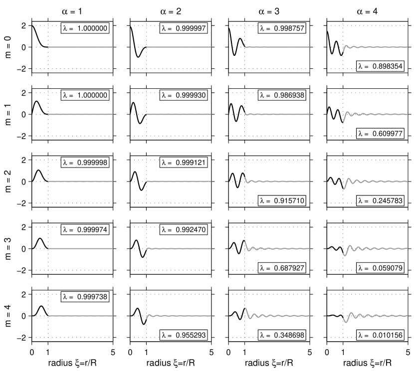
Figure 1: Radial dependence of the first four eigenfunctions of eq. (63), the bandlimited Slepian functions $\mathsf{g}_{\alpha}(r)$, $\alpha=1,2,3,4$, of fixed order $m=0$ (top) to $m=4$ (bottom), calculated from eq. (77) truncated at $l=84$. The Shannon number $N^{\mathrm{2D}}=42$ and the bandwidth $c\approx 13$. Black curves show the concentration within the scaled spatial interval $0\leq\xi\leq 1$ and grey curves show the leakage into the rest of the real line, which is truncated at $\xi=5$. Labels show the eigenvalues, $\lambda_{\alpha}$, calculated from eq. (79). These express the quality of the spatial concentration. Spacelimited, spectral-domain Slepian functions are shown in Fig. 2.

5.6 Numerical examples

With the eigenfunctions $\varphi(\xi)$ calculated, by series expansion de Villiers et al. (2003); Shkolnisky (2007) via eqs. (75) or (77) or even by quadrature Zhang (1994) of eq. (73), we rescale them following eqs. (72) and (65) to the Slepian functions $\mathsf{g}_{\alpha}(r)$ normalized according to (64). The sign is arbitrary: the concentration criterion is a quadratic.

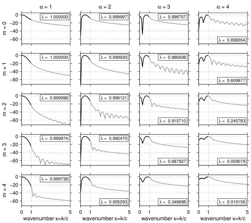
Figure 2: Squared Fourier coefficients $|H(k)|^{2}$ of the first four scaled spacelimited eigenfunctions $\mathsf{h}_{\alpha}(r)$, $\alpha=1,2,3,4$, of fixed order $m=0$ (top) to $m=4$ (bottom), calculated by discrete Fourier transformation of the functions shown by the thick black lines in Fig. 1. The Shannon number is $N^{\mathrm{2D}}=42$ and the scaled bandwidth $c\approx 13$. Black curves show the power within the scaled wavenumber interval $0\leq\kappa\leq 1$ and grey curves show the power leaked to the rest of the wavenumber axis, which is truncated at $\kappa=5$. Values of $|H(k)|^{2}$ are in decibel (dB), zero at the individual maxima. Labels show the eigenvalues $\lambda_{\alpha}$, which express the quality of the spectral concentration. The corresponding bandlimited, spatial-domain eigenfunctions are shown in Fig. 1.

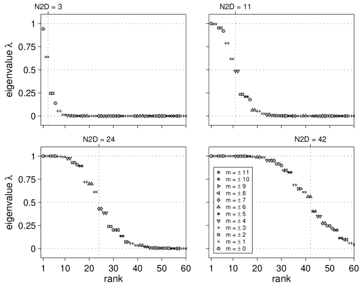
Figure 3: Eigenvalue spectra ($\lambda_{\alpha}$ versus rank $\alpha$) of the Cartesian concentration problem, at various Shannon numbers $N^{\mathrm{2D}}$, for disk-shaped regions, calculated via eq. (79). The total number of eigenvalues is unbounded; only $\lambda_{1}$ through $\lambda_{60}$ are shown. Different symbols are used to plot the various orders $-11\leq m\leq 11$; juxtaposed identical symbols are $\pm m$ doublets. Vertical grid lines and top labels specify the rounded Shannon numbers $N^{\mathrm{2D}}=3,11,24,42$.

The four most optimally concentrated eigenfunctions $\mathsf{g}_{1}(r),\mathsf{g}_{2}(r),\mathsf{g}_{3}(r),\mathsf{g}_{4}(r)$, for the orders $0\leq m\leq 4$ are plotted in Fig. 1, scaled for convenience. The associated eigenvalues $\lambda_{1},\lambda_{2},\lambda_{3},\lambda_{4}$ are listed to six-figure accuracy. The planar Shannon number in this example is $N^{\mathrm{2D}}=42$, hence $c\approx 13$. It is useful to compare the behavior of these solutions to those of the spherical concentration problem (Simons et al., 2006, Fig. 5.1), with which they are asymptotically self-similar Simons and Dahlen (2007); Simons et al. (2006). The first zeroth-order “zonal” ($m=0$) eigenfunction, $\mathsf{g}_{1}(r)$, has no nodes within the “cap” of radius $R$; the second, $\mathsf{g}_{2}(r)$, has one node, and so on. The non-zonal ($m>0$) eigenfunctions all vanish at the origin. The first three $m=0$, $m=1$ and $m=2$, and the first two $m=3$ and $m=4$ eigenfunctions are very well concentrated ($\lambda>0.9$). The fourth $m=3$ and $m=4$ eigenfunctions exhibit significant leakage ($\lambda<0.1$).

The squared Fourier coefficients $|H(k)|^{2}$ of the four best concentrated spacelimited eigenfunctions $\mathsf{h}_{1}(r),\mathsf{h}_{2}(r),\mathsf{h}_{3}(r),\mathsf{h}_{4}(r)$ for $0\leq m\leq 4$ are plotted versus scaled wavenumber $\kappa=k/c$, on a decibel scale, in Fig. 2. Shannon number, bandwidth, and layout are the same as in Fig. 1. See elsewhere (Simons et al., 2006, Fig. 5.2) to compare with the spherical case.

Once a number of sequences of fixed-order eigenvalues has been found, they can be resorted to an overall mixed-order ranking. The total number of significant eigenvalues is then given by eq. (70). In Fig. 3 we show the mixed-$m$ eigenvalue spectra for the Shannon numbers $N^{\mathrm{2D}}=3,11,24$ and $42$. These show the familiar step shape Landau (1965); Slepian and Sonnenblick (1965), with significant ($\lambda\approx 1$) and insignificant ($\lambda\approx 0$) eigenvalues separated by a narrow transition band. The Shannon numbers roughly separate the reasonably well concentrated eigensolutions ($\lambda\geq 0.5$) from the more poorly concentrated ones ($\lambda<0.5$) in all four cases. To compare with the spherical case, see elsewhere (Simons et al., 2006, Fig. 5.3).

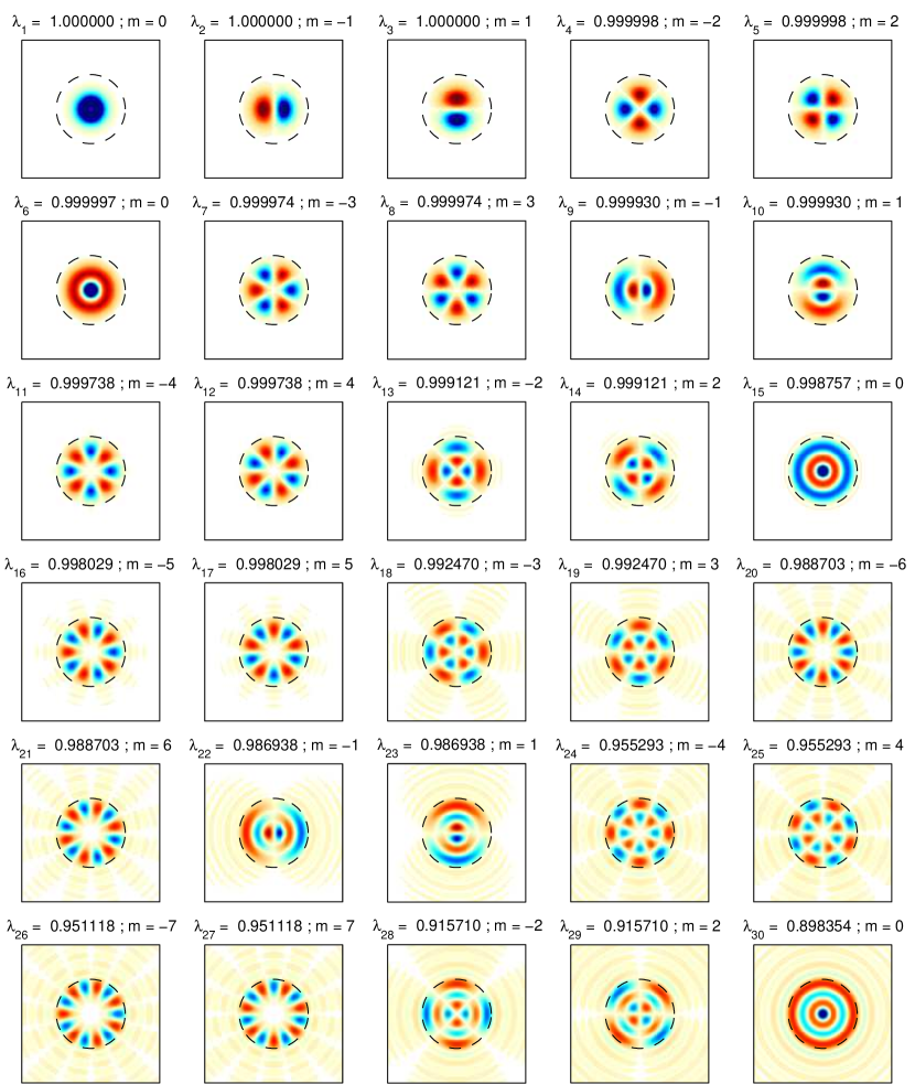
Figure 4: Bandlimited eigenfunctions $g(r,\theta)$ that are optimally concentrated within a disk of radius $R=1$. Dashed circle denotes the region boundary. The Shannon number $N^{\mathrm{2D}}=42$ and the scaled bandwidth $c\approx 13$. The eigenvalues $\lambda_{\alpha}$ have been sorted into a mixed-order ranking, $\alpha=1\rightarrow 30$, with the best concentrated eigenfunction plotted on the top left and the $30$th best on the lower right. Blue (or white in the print version) is positive and red (black in print) is negative; regions in which the absolute value is less than one hundredth of the maximum value on the domain are left white (grey at 50% in the print version).

Finally, Fig. 4 shows a polar plot of the first 30 eigenfunctions $g(r,\phi)$ concentrated within a radius $R=1$, defined by equations (62) using the $\mathsf{g}(r)$ shown in Fig. 1. The Shannon number is $N^{2D}=42$, as in Fig. 1. The eigenvalue ranking is mixed-order, as in Fig. 3, and all degenerate $\sqrt{2}\cos(m\phi),\sqrt{2}\sin(m\phi)$ doublets are shown. The concentration factors $1>\lambda\geq 0.8983$ and orders $m$ of each eigenfunction are indicated. Blue and red colors (in the online version; in print these have been converted to grey scales between white and black) represent positive and negative values, respectively; however, all signs could be reversed without violating the quadratic concentration criteria (34) and (42). Elsewhere (Simons et al., 2006, Fig. 5.4) these can be compared with the spherical case. Other calculation methods (see Sect. 6 below) may yield slight differences between what should be pairs of eigenvalues for each non-azimuthally symmetric and thus fixed non-zero order eigenfunction. The mismatch is confined to the last two quoted digits in a typical calculation (compare Simons, 2010, Fig. 2).

6 Computational Considerations on General Domains

While the framework of Sect. 4 is completely nonrestrictive as to the geometry of the spectral or spatial concentration regions $\mathcal{K}$ or $\mathcal{R}$, the literature treatment has remained focused on the cases with special symmetry that we discussed in Sect. 5, for which analytic solutions could be found. In what follows we lift all such restrictions and, numerically, solve the problem of finding the unknown planar function $f(\mathbf{x})$ that is bandlimited/band-concentrated to $\mathcal{K}$ and space-concentrated/spacelimited to $\mathcal{R}$, by satisfying the Fredholm eigenvalue equation

$$\int_{\mathcal{R}}D(\mathbf{x},\mathbf{x}^{\prime})\,f(\mathbf{x}^{\prime})\,d\mathbf{x}^{\prime}=\lambda\hskip 1.00006ptf(\mathbf{x}),$$ (80a)

$$D(\mathbf{x},\mathbf{x}^{\prime})=(2\pi)^{-2}\int_{\mathcal{K}}e^{i\mathbf{k}\cdot(\mathbf{x}-\mathbf{x}^{\prime})}\,d\mathbf{k},$$ (80b)

over the domains $\mathbf{x}\in\mathbb{R}^{2}$ (in which case we retrieve the bandlimited Slepian functions $g$ of Sect. 4.2) or $\mathbf{x}\in\mathcal{R}$ (when we obtain the spacelimited $h$ of Sect. 4.3).

6.1 Isotropic spectral response

Despite the appealing generality of eq. (80), applications in the geophysical or planetary sciences, e.g. in problems of spectral analysis of data collected on bounded geographical domains, is well served by Slepian functions whose spectral support is circularly isotropic. As we saw in Sect. 5.1, the integral kernel is then

$$D(\mathbf{x},\mathbf{x}^{\prime})=\frac{\displaystyle{K\hskip 1.00006ptJ_{1}(K\|\mathbf{x}-\mathbf{x}^{\prime}\|)}}{\displaystyle{2\pi\,\|\mathbf{x}-\mathbf{x}^{\prime}\|}}.$$ (81)

The standard solution to solve homogeneous Fredholm integral equations of the second kind is by the Nyström method Nyström (1930); Press et al. (1992).

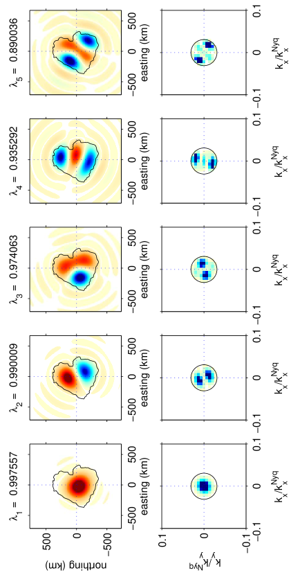
Figure 5: Bandlimited eigenfunctions $g_{1},g_{2},\ldots,g_{5}$, calculated by eq. (88) using Gauss-Legendre integration with 32 node points in both directions, optimally concentrated within the Colorado Plateaus, centered on 109.95^∘W 37.01^∘N (near Mexican Hat, Utah) of area $A\approx 334\times 10^{3}$ km². The concentration factors $\lambda_{1},\lambda_{2},\ldots,\lambda_{5}$ are indicated; the Shannon number is $N^{2D}=10$. The top row renders the eigenfunctions in space on a grid with 5 km resolution in both directions, with the reversible convention that positive values are blue (white in print) and negative values red (black in print). The spatial concentration region is outlined in black. The bottom row shows the squared Fourier coefficients $|G(\mathbf{k})|^{2}$ as calculated from the functions $g(\mathbf{x})$ shown, on a wavenumber scale that is expressed as a fraction of the Nyquist wavenumber. The spectral limitation region is shown by the black circle at wavenumber $K=0.0194$ rad/km. All areas for which the absolute value of the functions plotted is less than one hundredth of the maximum value attained over the domain are left white (grey at 50% in the print version).

In one dimension, let us write eq. (80) in a form reminiscent of the special case that we encountered previously in eq. (63), to which it also applies explicitly, namely

$$\int_{a}^{b}D(x,x^{\prime})\,f(x^{\prime})\,dx^{\prime}=\lambda\hskip 1.00006ptf(x).$$ (82)

The left-hand side of this equation is to be discretized by a quadrature rule; this involves choosing $J$ weights $w_{j}$ and abscissas $x_{j}$ such that, to the desired accuracy,

$$\int_{a}^{b}D(x,x^{\prime})\,f(x^{\prime})\,dx^{\prime}=\sum_{j=1}^{J}w_{j}D(x,x_{j})\,f(x_{j}),$$ (83)

using which we rewrite eq. (82) as

$$\sum_{j=1}^{J}w_{j}D(x_{i},x_{j})\,f(x_{j})=\lambda\hskip 1.00006ptf(x_{i}),$$ (84)

this time evaluating the unknown right hand side $f(x)$ at the quadrature points as well. Written in matrix form, we may solve

$$\mathbf{D}\cdot\mathbf{W}\cdot\mathbf{f}=\lambda\hskip 1.00006pt\mathbf{f},$$ (85)

identifying the elements of the square kernel $D_{ij}=D(x_{i},x_{j})$, the samples of the unknown function as $f_{j}=f(x_{j})$, and the entries of the diagonal weight matrix $W_{ij}=w_{j}\delta_{ij}$.

Restoring the symmetry of the problem contained in the symmetry $\mathbf{D}=\mathbf{D}^{\mathrm{\scriptstyle{T}}}$, and provided the weights $w_{j}$ are positive, we had rather solve

$$\mathbf{\tilde{W}}\cdot\mathbf{D}\cdot\mathbf{\tilde{W}}\cdot\mathbf{\tilde{f}}=\lambda\hskip 1.00006pt\mathbf{\tilde{f}},$$ (86)

using $\tilde{W}_{ij}=\sqrt{w_{i}}\delta_{ij}$ and $\mathbf{\tilde{f}}=\mathbf{\tilde{W}}\cdot\mathbf{f}$ or indeed $\tilde{f}_{i}=\sqrt{w_{i}}f_{i}$. Having solved this system for the unknown function $f(x_{i})$ at the integration nodes, we can subsequently produce either $g(x)$ (anywhere in one-dimensional space) or $h(x)$ (inside the region) using eqs. (82)–(83), to the same accuracy.

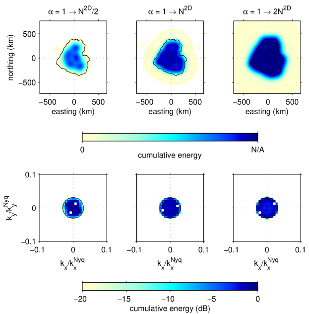
Figure 6: Cumulative eigenvalue-weighted energy of the first $N^{2D}/2,N^{2D}$ and $2N^{2D}$ eigenfunctions that are optimally concentrated within the Colorado Plateaus, with the Shannon number $N^{2D}=10$. The top row is in the spatial domain with the concentration region outlined in black. Darkest blue (white in print) on color bar corresponds to the expected value (58) of the sum, as shown. The bottom row is in the spectral domain with a wavenumber scale that is expressed as a fraction of the Nyquist wavenumber. The spectral limitation region is shown by the black circle. Areas with absolute value less than one hundredth of the maximum value attained over the domain are left white (grey at 50% in the print version).

In two dimensions, the vectors $\mathbf{x}=(x,y)$ and $\mathbf{x}^{\prime}=(x^{\prime},y^{\prime})$ denote points occupying the plane and eq. (80) is rewritten as

$$\int_{\mathcal{R}}D(\mathbf{x},\mathbf{x}^{\prime})\,f(\mathbf{x}^{\prime})\,d\mathbf{x}^{\prime}=\sum_{k=1}^{K}\sum_{l=1}^{L}w_{k}w_{l}D(\mathbf{x};x_{k},y_{l})\,f(x_{k},y_{l}),$$ (87)

where it is implied that $w_{l}=w_{l}(x_{k})$ and $y_{l}=y_{l}(x_{k})$. By wrapping the indices $k$ and $l$ on the scalar elements $x^{\prime}$ and $y^{\prime}$ into the vectorial indices $i$ and $j$ used for $\mathbf{x}$ and $\mathbf{x}^{\prime}$ we arrive at

$$\sum_{j=1}^{J}w^{\prime}_{j}D(\mathbf{x}_{i};\mathbf{x}_{j})\,f(\mathbf{x}_{j})=\lambda\hskip 1.00006ptf(\mathbf{x}_{i}).$$ (88)

This is identical to eq. (86) as long as we remember that the weights $w^{\prime}_{j}$ are pairwise products of the one-dimensional $w_{k}w_{l}$ and identifying $D_{ij}=D(\mathbf{x}_{i};\mathbf{x}_{j})$.

As to the choice of quadrature, a finely meshed Riemann sum might suffice for some applications Saito (2007); Zhang (1994), though we shall prefer the classical Gauss-Legendre algorithm Press et al. (1992) for increased accuracy at faster computation speeds. Other options are available as well Ramesh and Lean (1991). The analytical formulas for the special cases, e.g. eqs. (75), (77) and (79) can be used for verification purposes (see the discussion of Fig. 4 in the text), as we have.

Figures 5 and 6 were computed using eq. (88) with Gauss-Legendre quadrature, starting from a splined boundary of the Colorado Plateaus, a physiographic region in the United States. Fig. 5 shows the first five bandlimited Slepian functions, $g_{1}\rightarrow g_{5}$, with their eigenvalues, $\lambda_{1}\rightarrow\lambda_{5}$. The space-domain functions $g(\mathbf{x})$, shown in the top row, are increasingly oscillatory as their concentration values decrease. At the same time their periodograms $|G(\mathbf{k})|^{2}$, shown in the bottom row, remain strictly confined within the chosen isotropic spectral region of bandwidth $K$. All together, the Slepian functions uniformly occupy their respective domains of concentration or limitation. Fig. 6 shows the eigenvalue-weighted partial sums of the energy of the eigenfunctions, in space (top row) and spectral space (bottom row). The progressive covering behavior, consistent with eq. (58), lies at the basis of the success of the Slepian functions in being used as data tapers for spectral analysis Bronez (1988); Liu and van Veen (1992); Percival and Walden (1993): orthogonal over the domain that they cover, smoothly but rapidly decaying to zero at the boundary of interest, and with a finite and isotropic spectral response.

6.2 Arbitrary spectral response

We finally treat the situation in which both the spatial and spectral concentration domains are of arbitrary description — but with Hermitian spectral symmetry, see eqs. (28)–(29), if the Slepian functions are to be real-valued. No analytical results can be expected for such a case, and we benefit from writing the concentration problem in its most abstract form. Writing $\mathcal{Q}$ for the operator that acts on a spatial function $f(\mathbf{x})$ to return its Fourier transform $F(\mathbf{k})$, we introduce the spatial projection operator

$$\mathcal{P}f(\mathbf{x})=\left\{\begin{array}[]{ll}f(\mathbf{x})&\mbox{if $\mathbf{x}\in\mathcal{R}$,}\\ 0&\mbox{otherwise},\end{array}\right.$$ (89)

and the spectral projection operator

$$\mathcal{L}F(\mathbf{k})=\left\{\begin{array}[]{ll}F(\mathbf{k})&\mbox{if $\mathbf{k}\in\mathcal{K}$,}\\ 0&\mbox{otherwise}.\end{array}\right.$$ (90)

We rewrite the variational equations (34) and (42) in inner-product notation as

$$\lambda=\frac{\displaystyle{\langle\mathcal{P}\mathcal{Q}^{-1}\!\mathcal{L}F,\mathcal{P}\mathcal{Q}^{-1}\!\mathcal{L}F\rangle}}{\displaystyle{\langle\mathcal{Q}^{-1}\!\mathcal{L}F,\mathcal{Q}^{-1}\!\mathcal{L}F\rangle}}=\frac{\displaystyle{\langle\mathcal{L}\mathcal{Q}\mathcal{P}f,\mathcal{L}\mathcal{Q}\mathcal{P}f\rangle}}{\displaystyle{\langle\mathcal{Q}\mathcal{P}f,\mathcal{Q}\mathcal{P}f\rangle}}=\mbox{maximum}.$$ (91)

The associated spectral-domain and spatial-domain eigenvalue equations are

$$\mathcal{L}\mathcal{Q}\mathcal{P}\mathcal{Q}^{-1}\!\mathcal{L}(\mathcal{L}F)=\lambda\hskip 0.50003pt(\mathcal{L}F),\qquad\mathcal{P}\mathcal{Q}^{-1}\!\mathcal{L}\mathcal{Q}\mathcal{P}(\mathcal{P}f)=\lambda\hskip 0.50003pt(\mathcal{P}f),$$ (92)

where we have made use of the fact that $\mathcal{P}^{2}=\mathcal{P}$ and $\mathcal{L}^{2}=\mathcal{L}$ are self-adjoint, and that $\mathcal{Q}$ and $\mathcal{Q}^{-1}\!$ are each other’s adjoints, provided we rewrite eq. (28) as a unitary transform. In our notation, the solutions $\mathcal{L}F$ yield the Fourier transforms of the bandlimited functions $g(\mathbf{x})$ of Sect. 4.2, while the $\mathcal{P}f$ represent the spacelimited functions $h(\mathbf{x})$ of Sect. 4.3.

For computation in the discrete-discrete case, $\mathcal{P}$ and $\mathcal{L}$ will simply be matrices of ones and zeros, and $\mathcal{Q}$ and $\mathcal{Q}^{-1}\!$ will be the discrete Fourier transform (DFT) matrix and its conjugate transpose. Both $\mathcal{L}\mathcal{Q}\mathcal{P}\mathcal{Q}^{-1}\!\mathcal{L}$ and $\mathcal{P}\mathcal{Q}^{-1}\!\mathcal{L}\mathcal{Q}\mathcal{P}$ will be Hermitian and typically sparse, hence a number of dedicated eigenvalues solvers can be used to find the Slepian functions. In our own Matlab implementation we furthermore take advantage of defining the operators as “anonymous” functions. This greatly improves the performance of the resulting algorithm, which we tested by comparison with the methods available for the special cases discussed in Sections 2 and 5. With this we have complete liberty to design Slepian functions on geographical domains, including the ability to construct “steerable”, anisotropic windows for texture-sensitive analysis that is of interest in theory Olhede and Metikas (2009); van de Ville and Unser (2008) and practice Audet and Mareschal (2007); Kirby and Swain (2006). Fig. 7 shows two numerical examples of Slepian functions $h$ spectrally sensitive in wedge-shaped oriented domains. The top row shows $h_{1}\rightarrow h_{4}$ and their eigenvalues, $\lambda_{1}\rightarrow\lambda_{4}$, followed by eigenvalue-weighted sums of their periodograms, $\sum_{\alpha=1}^{20}\lambda_{\alpha}|H_{\alpha}(\mathbf{k})|^{2}$, on a decibel scale. These are orientated at $\pi/6$ from the horizontal. The bottom row shows the equivalent results oriented at $-\pi/6$ from the horizontal. Both cases were computed by diagonalization (eigs) of the operator $\mathcal{P}\mathcal{Q}^{-1}\!\mathcal{L}\mathcal{Q}\mathcal{P}$ whereby $\mathcal{Q}$ is the anonymous function call to the two-dimensional Fast Fourier Transform (fft2) and $\mathcal{Q}^{-1}\!$ its inverse (ifft2). This immediately returns the $h(\mathbf{x})$ on a discretized calculation domain in which, once again, the region of the Colorado Plateaus was embedded. The functions $h_{1}\rightarrow h_{4}$ shown are the real parts of the eigensolutions associated with the four eigenvalues $\lambda_{1}\rightarrow\lambda_{4}$ that have the largest real part. The eigenvalues of these “generalized prolate spheroidal data sequences” (gpss), which need not in principle be defined on regularly sampled grids Bronez (1988), are sensitive to the discretization and the size of the computational domains to which the inner products in eq. (91) refer. The slightly different manner in which these sample the parametrically defined rotated spectral concentration domains explains the discrepancy of the eigenvalues between the two cases that are shown in the top and bottom rows of Fig. 7.

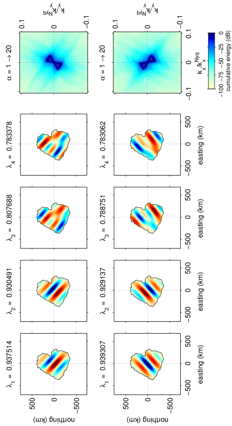
Figure 7: Two sets of eigenfunctions $h_{1},h_{2},\ldots,h_{4}$ that are strictly spacelimited within the Colorado Plateaus and optimally concentrated within a wedge-shaped spectral domain, with their concentration factors $\lambda_{1},\lambda_{2},\ldots,\lambda_{4}$. The last panel on each row shows the eigenvalue-weighted periodograms of the first $\alpha=1\rightarrow 20$ eigenfunctions. The functions $h(\mathbf{x})=\mathcal{P}f(\mathbf{x})$ were calculated by diagonalization of the spatial-domain operator equation (92) on a domain that we took to be three times the size of the box inscribing the concentration domain outlined in black, discretized on a 5$\times$5 km² grid. The spectral concentration domains are triangles with Hermitian symmetry oriented at $\pm\pi/6$ from the horizontal in the top and bottom rows, respectively.

7 Conclusion

Slepian functions are orthogonal families of functions that are all defined on a common spatial domain, where they are either optimally concentrated or within which they are exactly limited. At the same time they are exactly confined within a certain spectral interval, or maximally concentrated therein Simons (2010). The joint optimization of quadratic spatio-spectral concentration is generally referred to as Slepian’s problem, which we encountered as eq. (3) in one dimension, as eq. (15) on the surface of a sphere, and as eq. (34) in two Cartesian dimensions. Without qualification in one, and under special symmetry considerations in multiple dimensions, Slepian functions solve Sturm–Liouville equations, notably eqs. (11), (3), (3) and (74). In those cases (though on the sphere only asymptotically) the solutions depend on the spatial and spectral areas of concentration only through the Shannon number, which depends on their product, as defined by eqs. (9), (3) and (56). More generally, they solve Fredholm integral equations in their respective dimensions, as exemplified by eqs. (5), (17), and (38).

What unites the Slepian functions is that the kernels of the integral equations they solve are best thought of in the context of reproducing-kernel Hilbert spaces Amirbekyan et al. (2008); Nashed and Walter (1991); Yao (1967). Each of $D(t,t^{\prime})$ in eq. (5b), $D(\mathbf{\hat{r}},\mathbf{\hat{r}}^{\prime})$ in eq. (17b) and $D(\mathbf{x},\mathbf{x}^{\prime})$ in eq. (38b), is a restriction of the traditional Dirac delta functions, $\delta(t,t^{\prime})$, $\delta(\mathbf{\hat{r}},\mathbf{\hat{r}}^{\prime})$, and $\delta(\mathbf{x},\mathbf{x}^{\prime})$, to a region of finite bandwidth Simons (2010). While the latter satisfy, for any square-integrable function $f$, the relations

$$f(t) = \int_{-\infty}^{\infty}f(t^{\prime})\hskip 1.00006pt\delta(t,t^{\prime})\,dt^{\prime},$$ (93a)

$$f(\mathbf{x}) = \int_{\mathbb{R}^{2}}f(\mathbf{x}^{\prime})\hskip 1.00006pt\delta(\mathbf{x},\mathbf{x}^{\prime})\,d\mathbf{x}^{\prime},$$ (93b)

$$f(\mathbf{\hat{r}}) = \int_{\Omega}f(\mathbf{\hat{r}}^{\prime})\hskip 1.00006pt\delta(\mathbf{\hat{r}},\mathbf{\hat{r}}^{\prime})\,d\Omega^{\prime},$$ (93c)

the former act on functions $g$ that belong to appropriately bandlimited subspaces, as we have defined them in eqs. (2), (14) and (33), in much the same way:

$$g(t) = \int_{-\infty}^{\infty}g(t^{\prime})D(t,t^{\prime})\,dt^{\prime},$$ (94a)

$$g(\mathbf{x}) = \int_{\mathbb{R}^{2}}g(\mathbf{x}^{\prime})D(\mathbf{x},\mathbf{x}^{\prime})\,d\mathbf{x}^{\prime},$$ (94b)

$$g(\mathbf{\hat{r}}) = \int_{\Omega}g(\mathbf{\hat{r}}^{\prime})D(\mathbf{\hat{r}},\mathbf{\hat{r}}^{\prime})\,d\Omega.$$ (94c)

Note that these are not equal to eqs. (5), (17), or (38). Hence the $g$ are a basis for bandlimited processes anywhere on the applicable domain ($\mathbb{R}$, $\mathbb{R}^{2}$ or the entire spherical surface $\Omega$) Daubechies (1992); Flandrin (1998); Freeden et al. (1998); Landau and Pollak (1961); Slepian and Pollak (1961). Therein, the Shannon-number best time- or space-concentrated members allow for sparse, approximate expansions of signals that are concentrated to the spatial region of choice. Similarly, the infinite sets of exactly time- or spacelimited (and thus band-concentrated) functions $h$ which are the eigenfunctions of eqs. (5), (17) and (38) with the domains appropriately restricted, see eq. (45) for the two-dimensional case, are complete bases for square-integrable scalar functions on the intervals to which they are confined Landau and Pollak (1961); Simons et al. (2006); Slepian and Pollak (1961). Expansions of wideband but spectrally concentrated signals in the small subset of their Shannon-number most band-concentrated members provide approximations which are spectrally faithful and constructive as their numbers grow Simons (2010); Simons et al. (2009).

Slepian functions defined on two-dimensional Cartesian domains are of great utility in the natural sciences. Despite this, no comprehensive prior treatment was available, beyond that of cases for regions with advanced symmetry. The present paper has attempted to do right by, especially, the geosciences, where Fourier-based methods and analyses are often required but the domains of interest are rarely circles or rectangles. Much can be learned from those special cases, however, including from the one-dimensional and spherical situations that we have reviewed also. Most particularly, they have helped us test and benchmark the algorithms that we have discussed and are making available on the Web as part of this publication. In having ended Sect. 6 with a computational procedure for the design of planar Cartesian Slepian functions on arbitrarily irregular spatial and spectral domains, which could be captured in just a few lines, see eqs. (89)–(92), and carried out in a handful of lines of Matlab code, we believe to have returned to a level of practicality that should appeal to researchers across a wide spectrum.

References

- Abramowitz and Stegun (1965) Abramowitz, M., and I. A. Stegun, Handbook of Mathematical Functions, Dover, New York, 1965.
- Albertella and Sacerdote (2001) Albertella, A., and F. Sacerdote, Using Slepian functions for local geodetic computations, Boll. Geod. Sc. Aff., 60(1), 1–14, 2001.
- Albertella et al. (1999) Albertella, A., F. Sansò, and N. Sneeuw, Band-limited functions on a bounded spherical domain: the Slepian problem on the sphere, J. Geodesy, 73, 436–447, 1999.
- Amirbekyan et al. (2008) Amirbekyan, A., V. Michel, and F. J. Simons, Parameterizing surface-wave tomopgraphic models with harmonic spherical splines, Geophys. J. Int., 174(2), 617, doi: 10.1111/j.1365–246X.2008.03,809.x, 2008.
- Aronszajn (1950) Aronszajn, N., Theory of reproducing kernels, Trans. Am. Math. Soc., 68(3), 337–404, 1950.
- Audet and Mareschal (2007) Audet, P., and J.-C. Mareschal, Wavelet analysis of the coherence between Bouguer gravity and topography: application to the elastic thickness anisotropy in the Canadian Shield, Geophys. J. Int., 168, 287–298, doi: 10.1111/j.1365–246X.2006.03,231.x, 2007.
- Bell et al. (1993) Bell, B., D. B. Percival, and A. T. Walden, Calculating Thomson’s spectral multitapers by inverse iteration, J. Comp. Graph. Stat., 2(1), 119–130, 1993.
- Bertero et al. (1985a) Bertero, M., C. de Mol, and E. R. Pike, Linear inverse problems with discrete data. I. General formulation and singular system analysis, Inv. Probl., 1, 301–330, doi: 10.1088/0266–5611/1/4/004, 1985a.
- Bertero et al. (1985b) Bertero, M., C. de Mol, and E. R. Pike, Linear inverse problems with discrete data. II. Stability and regularisation, Inv. Probl., 1, 301–330, doi: 10.1088/0266–5611/1/4/004, 1985b.
- Beylkin and Monzón (2002) Beylkin, G., and L. Monzón, On generalized Gaussian quadratures for exponentials and their applications, Appl. Comput. Harmon. Anal., 12, 332–372, doi: 10.1006/acha.2002.0380, 2002.
- Beylkin and Sandberg (2005) Beylkin, G., and K. Sandberg, Wave propagation using bases for bandlimited functions, Wave Motion, 41(3), 263–291, 2005.
- Borcea et al. (2008) Borcea, L., G. Papanicolaou, and F. G. Vasquez, Edge illumination and imaging of extended reflectors, SIAM J. Imag. Sci., 1(1), 75–114, doi:10.1137/07069,290X, 2008.
- Bouwkamp (1947) Bouwkamp, C. J., On spheroidal wave functions of order zero, J. Math. Phys., 26, 79–92, 1947.
- Boyd (2003) Boyd, J. P., Approximation of an analytic function on a finite real interval by a bandlimited function and conjectures on properties of prolate spheroidal functions, Appl. Comput. Harmon. Anal., 15(2), 168–176, 2003.
- Boyd (2004) Boyd, J. P., Prolate spheroidal wavefunctions as an alternative to Chebyshev and Legendre polynomials for spectral element and pseudospectral algorithms, J. Comput. Phys., 199(2), 688–716, 2004.
- Brander and DeFacio (1986) Brander, O., and B. DeFacio, A generalisation of Slepian’s solution for the singular value decomposition of filtered Fourier transforms, Inv. Probl., 2, L9–L14, 1986.
- Bronez (1988) Bronez, T. P., Spectral estimation of irregularly sampled multidimensional processes by generalized prolate spheroidal sequences, IEEE Trans. Acoust. Speech Signal Process., 36(12), 1862–1873, 1988.
- Chambodut et al. (2005) Chambodut, A., I. Panet, M. Mandea, M. Diament, M. Holschneider, and O. Jamet, Wavelet frames: an alternative to spherical harmonic representation of potential fields, Geophys. J. Int., 163(3), 875–899, 2005.
- Chen et al. (2005) Chen, Q. Y., D. Gottlieb, and J. S. Hesthaven, Spectral methods based on prolate spheroidal wave functions for hyperbolic PDEs, Wave Motion, 43(5), 1912–1933, 2005.
- Coifman and Lafon (2006) Coifman, R. R., and S. Lafon, Geometric harmonics: A novel tool for multiscale out-of-sample extension of empirical functions, Appl. Comput. Harmon. Anal., 21, 31–52, doi: 10.1016/j.acha.2005.07.005, 2006.
- Dahlen and Simons (2008) Dahlen, F. A., and F. J. Simons, Spectral estimation on a sphere in geophysics and cosmology, Geophys. J. Int., 174, 774–807, doi: 10.1111/j.1365–246X.2008.03,854.x, 2008.
- Dahlen and Tromp (1998) Dahlen, F. A., and J. Tromp, Theoretical Global Seismology, Princeton Univ. Press, Princeton, N. J., 1998.
- Daubechies (1988) Daubechies, I., Time-frequency localization operators: A geometric phase space approach, IEEE Trans. Inform. Theory, 34, 605–612, 1988.
- Daubechies (1992) Daubechies, I., Ten Lectures on Wavelets, CBMS-NSF Regional Conference Series in Applied Mathematics, vol. 61, Society for Industrial & Applied Mathematics, Philadelphia, Penn., 1992.
- Daubechies and Paul (1988) Daubechies, I., and T. Paul, Time-frequency localisation operators — A geometric phase space approach: II. The use of dilations, Inv. Probl., 4(3), 661–680, 1988.
- de Villiers et al. (2001) de Villiers, G. D., F. B. T. Marchaud, and E. R. Pike, Generalized Gaussian quadrature applied to an inverse problem in antenna theory, Inverse Problems, 17, 1163–1179, 2001.
- de Villiers et al. (2003) de Villiers, G. D., F. B. T. Marchaud, and E. R. Pike, Generalized Gaussian quadrature applied to an inverse problem in antenna theory: II. The two-dimensional case with circular symmetry, Inverse Problems, 19, 755–778, 2003.
- Delsarte et al. (1985) Delsarte, P., A. J. E. M. Janssen, and L. B. Vries, Discrete prolate spheroidal wave functions and interpolation, SIAM J. Appl. Math., 45(4), 641–650, 1985.
- Donoho and Stark (1989) Donoho, D. L., and P. B. Stark, Uncertainty principles and signal recovery, SIAM J. Appl. Math., 49(3), 906–931, 1989.
- Edmonds (1996) Edmonds, A. R., Angular Momentum in Quantum Mechanics, Princeton Univ. Press, Princeton, N.J., 1996.
- Evans et al. (2010) Evans, A. J., J. C. Andrews-Hanna, and M. T. Zuber, Geophysical limitations on the erosion history within Arabia Terra, J. Geophys. Res., 115, E05,007, doi: 10.1029/2009JE003,469, 2010.
- Faÿ et al. (2008) Faÿ, G., F. Guilloux, M. Betoule, J.-F. Cardoso, J. Delabrouille, and M. L. Jeune, CMB power spectrum estimation using wavelets, Phys. Rev. D, 78, 083,013, doi: 10.1103/PhysRevD.78.083,013, 2008.
- Fengler et al. (2007) Fengler, M. J., W. Freeden, A. Kohlhaas, V. Michel, and T. Peters, Wavelet modeling of regional and temporal variations of the earth’s gravitational potential observed by GRACE, J. Geodesy, 81(1), 5–15, doi: 10.1007/s00,190–006–0040–1, 2007.
- Flandrin (1998) Flandrin, P., Temps-Fréquence, 2 ed., Hermès, Paris, 1998.
- Freeden and Michel (1999) Freeden, W., and V. Michel, Constructive approximation and numerical methods in geodetic research today – an attempt at a categorization based on an uncertainty principle, J. Geodesy, 73(9), 452–465, 1999.
- Freeden and Windheuser (1997) Freeden, W., and U. Windheuser, Combined spherical harmonic and wavelet expansion — A future concept in Earth’s gravitational determination, Appl. Comput. Harmon. Anal., 4, 1–37, 1997.
- Freeden et al. (1998) Freeden, W., T. Gervens, and M. Schreiner, Constructive Approximation on the Sphere, Clarendon Press, Oxford, UK, 1998.
- Golub and van Loan (1989) Golub, G. H., and C. F. van Loan, Matrix Computations, 2nd ed., Johns Hopkins Univ. Press, Baltimore, Md., 1989.
- Gradshteyn and Ryzhik (2000) Gradshteyn, I. S., and I. M. Ryzhik, Tables of Integrals, Series, and Products, 6 ed., Academic Press, San Diego, Calif., 2000.
- Grünbaum (1981) Grünbaum, F. A., Eigenvectors of a Toeplitz matrix: discrete version of the prolate spheroidal wave functions, SIAM J. Alg. Disc. Meth., 2(2), 136–141, 1981.
- Grünbaum et al. (1982) Grünbaum, F. A., L. Longhi, and M. Perlstadt, Differential operators commuting with finite convolution integral operators: some non-Abelian examples, SIAM J. Appl. Math., 42(5), 941–955, 1982.
- Hall and Mitchell (2002) Hall, B. C., and J. J. Mitchell, Coherent states on spheres, J. Math. Phys., 43(3), 1211–1236, 2002.
- Han (2008) Han, S.-C., Improved regional gravity fields on the Moon from Lunar Prospector tracking data by means of localized spherical harmonic functions, J. Geophys. Res., 113, E11,012, doi:10.1029/2008JE003,166, 2008.
- Han and Ditmar (2007) Han, S.-C., and P. Ditmar, Localized spectral analysis of global satellite gravity fields for recovering time-variable mass redistributions, J. Geodesy, 82(7), 423–430, doi: 10.1007/s00,190–007–0194–5, 2007.
- Han and Simons (2008) Han, S.-C., and F. J. Simons, Spatiospectral localization of global geopotential fields from the Gravity Recovery and Climate Experiment GRACE reveals the coseismic gravity change owing to the 2004 Sumatra-Andaman earthquake, J. Geophys. Res., 113, B01,405, doi: 10.1029/2007JB004,927, 2008.
- Han et al. (2008a) Han, S.-C., D. D. Rowlands, S. B. Luthcke, and F. G. Lemoine, Localized analysis of satellite tracking data for studying time-variable Earth’s gravity fields, J. Geophys. Res., 113, B06,401, doi: 10.1029/2007JB005,218, 2008a.
- Han et al. (2008b) Han, S.-C., J. Sauber, S. B. Luthcke, C. Ji, and F. F. Pollitz, Implications of postseismic gravity change following the great 2004 Sumatra-Andaman earthquake from the regional harmonic analysis of GRACE inter-satellite tracking data, J. Geophys. Res., 113, B11,413, doi: 10.1029/2008JB005,705, 2008b.
- Han et al. (2009) Han, S.-C., E. Mazarico, and F. G. Lemoine, Improved nearside gravity field of the Moon by localizing the power law constraint, Geophys. Res. Lett., 36, L11,203, doi:10.1029/2009GL038,556, 2009.
- Hanssen (1997) Hanssen, A., Multidimensional multitaper spectral estimation, Signal Process., 58, 327–332, 1997.
- Harig et al. (2010) Harig, C., S. Zhong, and F. J. Simons, Constraints on upper-mantle viscosity inferred from the flow-induced pressure gradient across a continental keel, Geochem. Geophys. Geosys., 11(6), Q06,004, doi: 10.1029/2010GC003,038, 2010.
- Holschneider et al. (2003) Holschneider, M., A. Chambodut, and M. Mandea, From global to regional analysis of the magnetic field on the sphere using wavelet frames, Phys. Earth Planet. Inter., 135, 107–124, 2003.
- Jackson et al. (1991) Jackson, J. I., C. H. Meyer, D. G. Nishimura, and A. Macovski, Selection of a convolution function for Fourier inversion using gridding, IEEE Trans. Med. Imag., 10(3), 473–478, 1991.
- Jeffreys and Jeffreys (1988) Jeffreys, H., and B. S. Jeffreys, Methods of Mathematical Physics, 3 ed., Cambridge Univ. Press, Cambridge, UK, 1988.
- Karoui and Moumni (2008) Karoui, A., and T. Moumni, New efficient methods of computing the prolate spheroidal wave functions and their corresponding eigenvalues, Appl. Comput. Harmon. Anal., 24(3), 269–289, 2008.
- Kennedy et al. (2008) Kennedy, R. A., W. Zhang, and T. D. Abhayapala, Spherical harmonic analysis and model-limited extrapolation on the sphere: Integral equation formulation, in Proc. IEEE Int. Conf. Signal Process. Comm. Syst., pp. 1–6, doi: 10.1109/ICSPCS.2008.4813,702, IEEE, 2008.
- Khare and George (2003) Khare, K., and N. George, Sampling theory approach to prolate spheroidal wavefunctions, J. Phys. A: Math. Gen., 36, 10,011–10,021, 2003.
- Kido et al. (2003) Kido, M., D. A. Yuen, and A. P. Vincent, Continuous wavelet-like filter for a spherical surface and its application to localized admittance function on Mars, Phys. Earth Planet. Inter., 135, 1–14, 2003.
- Kirby and Swain (2006) Kirby, J. F., and C. J. Swain, Mapping the mechanical anisotropy of the lithosphere using a 2D wavelet coherence, and its application to Australia, Phys. Earth Planet. Inter., 158(2–4), 122–138, doi: 10.1016/j.pepi.2006.03.022, 2006.
- Kowalski and Rembieliński (2000) Kowalski, K., and J. Rembieliński, Quantum mechanics on a sphere and coherent states, J. Phys. A: Math. Gen., 33, 6035–6048, 2000.
- Lai et al. (2009) Lai, M. J., C. K. Shum, V. Baramidze, and P. Wenston, Triangulated spherical splines for geopotential reconstruction, J. Geod., 83, 695–708, doi: 10.1007/s00,190–008–0283–0, 2009.
- Landau (1965) Landau, H. J., On the eigenvalue behavior of certain convolution equations, Trans. Am. Math. Soc., 115, 242–256, 1965.
- Landau and Pollak (1961) Landau, H. J., and H. O. Pollak, Prolate spheroidal wave functions, Fourier analysis and uncertainty — II, Bell Syst. Tech. J., 40(1), 65–84, 1961.
- Landau and Pollak (1962) Landau, H. J., and H. O. Pollak, Prolate spheroidal wave functions, Fourier analysis and uncertainty — III: The dimension of the space of essentially time- and band-limited signals, Bell Syst. Tech. J., 41(4), 1295–1336, 1962.
- Lilly and Park (1995) Lilly, J. M., and J. Park, Multiwavelet spectral and polarization analyses of seismic records, Geophys. J. Int., 122, 1001–1021, 1995.
- Lindquist et al. (2006) Lindquist, M. A., C. H. Zhang, G. Glover, L. Shepp, and Q. X. Yang, A generalization of the two-dimensional prolate spheroidal wave function method for nonrectilinear MRI data acquisition methods, IEEE Trans. Image Proc., 15(9), 2792–2804, doi: 10.1109/TIP.2006.877,314, 2006.
- Liu and van Veen (1992) Liu, T.-C., and B. D. van Veen, Multiple window based minimum variance spectrum estimation for multidimensional random fields, IEEE Trans. Signal Process., 40(3), 578–589, doi: 10.1109/78.120,801, 1992.
- Ma et al. (1996) Ma, J., V. Rokhlin, and S. Wandzura, Generalized Gaussian quadrature rules for systems of arbitrary functions, SIAM J. Numer. Anal., 33(3), 971–996, 1996.
- Mallat (1998) Mallat, S., A Wavelet Tour of Signal Processing, Academic Press, San Diego, Calif., 1998.
- Maniar and Mitra (2005) Maniar, H., and P. P. Mitra, The concentration problem for vector fields, Int. J. Bioelectromagn., 7(1), 142–145, 2005.
- Marinucci et al. (2008) Marinucci, D., D. Pietrobon, A. Balbi, P. Baldi, P. Cabella, G. Kerkyacharian, P. Natoli, Picard, and N. Vittorio, Spherical needlets for cosmic microwave background data analysis, Mon. Not. R. Astron. Soc, 383(2), 539–545, doi: 10.1111/j.1365–2966.2007.12,550.x, 2008.
- McEwen et al. (2007) McEwen, J. D., M. P. Hobson, D. J. Mortlock, and A. N. Lasenby, Fast directional continuous spherical wavelet transform algorithms, IEEE Trans. Signal Process., 55(2), 520–529, 2007.
- Michel and Wolf (2008) Michel, V., and K. Wolf, Numerical aspects of a spline-based multiresolution recovery of the harmonic mass density out of gravity functionals, Geophys. J. Int., 173, 1–16, doi: 10.1111/j.1365–246X.2007.03,700.x, 2008.
- Miranian (2004) Miranian, L., Slepian functions on the sphere, generalized Gaussian quadrature rule, Inv. Prob., 20, 877–892, 2004.
- Mitra and Maniar (2006) Mitra, P. P., and H. Maniar, Concentration maximization and local basis expansions (LBEX) for linear inverse problems, IEEE Trans. Biomed Eng., 53(9), 1775–1782, 2006.
- Moore and Cada (2004) Moore, I. C., and M. Cada, Prolate spheroidal wave functions, an introduction to the Slepian series and its properties, Appl. Comput. Harmon. Anal., 16, 208–230, 2004.
- Narcowich and Ward (1996) Narcowich, F. J., and J. D. Ward, Nonstationary wavelets on the m-sphere for scattered data, Appl. Comput. Harmon. Anal., 3, 324–336, 1996.
- Nashed and Walter (1991) Nashed, M. Z., and G. G. Walter, General sampling theorems for functions in Reproducing Kernel Hilbert Spaces, Math. Control Signals Syst., 4, 363–390, 1991.
- Nyström (1930) Nyström, E. J., Über die praktische Auflösung von Integralgleichungen mit Anwendungen auf Randwertaufgaben, Acta Mathematica, 54, 185–204, 1930.
- Olhede and Walden (2002) Olhede, S., and A. T. Walden, Generalized Morse wavelets, IEEE Trans. Signal Process., 50(11), 2661–2670, 2002.
- Olhede and Metikas (2009) Olhede, S. C., and G. Metikas, The monogenic wavelet transform, IEEE Trans. Signal Process., 57(9), 3426–3441, doi: 10.1109/TSP.2009.2023,397, 2009.
- Panet et al. (2006) Panet, I., A. Chambodut, M. Diament, M. Holschneider, and O. Jamet, New insights on intraplate volcanism in French Polynesia from wavelet analysis of GRACE, CHAMP, and sea surface data, J. Geophys. Res., 111, B09,403, doi: 10.1029/2005JB004,141, 2006.
- Papoulis (1975) Papoulis, A., A new algorithm in spectral analysis and band-limited extrapolation, IEEE-CS, 22(9), 735–742, 1975.
- Parks and Shenoy (1990) Parks, T. W., and R. G. Shenoy, Time-frequency concentrated basis functions, in Proc. IEEE Int. Conf. Acoust. Speech Signal Process., vol. 5, pp. 2459–2462, IEEE, 1990.
- Parlett and Wu (1984) Parlett, B. N., and W.-D. Wu, Eigenvector matrices of symmetric tridiagonals, Numer. Math., 44, 103–110, 1984.
- Percival and Walden (1993) Percival, D. B., and A. T. Walden, Spectral Analysis for Physical Applications, Multitaper and Conventional Univariate Techniques, Cambridge Univ. Press, New York, 1993.
- Percival and Walden (2006) Percival, D. B., and A. T. Walden, Wavelet methods for time series analysis, Cambridge Univ. Press, 2006.
- Press et al. (1992) Press, W. H., S. A. Teukolsky, W. T. Vetterling, and B. P. Flannery, Numerical Recipes in FORTRAN: The Art of Scientific Computing, 2nd ed., Cambridge Univ. Press, New York, 1992.
- Ramesh and Lean (1991) Ramesh, P. S., and M. H. Lean, Accurate integration of singular kernels in boundary integral formulations for Helmholtz equation, Int. J. Num. Meth. Eng., 31, 1055–1068, 1991.
- Riedel and Sidorenko (1995) Riedel, K. S., and A. Sidorenko, Minimum bias multiple taper spectral estimation, IEEE Trans. Signal Process., 43(1), 188–195, 1995.
- Saito (2007) Saito, N., Data analysis and representation on a general domain using eigenfunctions of Laplacian, Appl. Comput. Harmon. Anal., 25, 68–97, doi: 10.1016/j.acha.2007.09.005, 2007.
- Schmidt et al. (2006) Schmidt, M., S.-C. Han, J. Kusche, L. Sanchez, and C. K. Shum, Regional high-resolution spatiotemporal gravity modeling from GRACE data using spherical wavelets, Geophys. Res. Lett., 33(8), L0840, doi: 10.1029/2005GL025,509, 2006.
- Schmidt et al. (2007) Schmidt, M., M. Fengler, T. Mayer-Gürr, A. Eicker, J. Kusche, L. Sánchez, and S.-C. Han, Regional gravity modeling in terms of spherical base functions, J. Geodesy, 81(1), 17–38, doi: 10.1007/s00,190–006–0101–5, 2007.
- Schott and Thébault (2011) Schott, J.-J., and E. Thébault, Modelling the earth’s magnetic field from global to regional scales, in Geomagnetic Observations and Models, IAGA Special Sopron Book Ser., vol. 5, edited by M. Mandea and M. Korte, Springer, 2011.
- Shepp and Zhang (2000) Shepp, L., and C.-H. Zhang, Fast functional magnetic resonance imaging via prolate wavelets, Appl. Comput. Harmon. Anal., 9(2), 99–119, doi: 10.1006/acha.2000.0302, 2000.
- Shkolnisky (2007) Shkolnisky, Y., Prolate spheroidal wave functions on a disc — Integration and approximation of two-dimensional bandlimited functions, Appl. Comput. Harmon. Anal., 22, 235–256, doi: 10.1016/j.acha.2006.07.002, 2007.
- Shkolnisky et al. (2006) Shkolnisky, Y., M. Tygert, and V. Rokhlin, Approximation of bandlimited functions, Appl. Comput. Harmon. Anal., 21, 413–420, doi: 10.1016/j.acha.2006.05.001, 2006.
- Simons (2010) Simons, F. J., Slepian functions and their use in signal estimation and spectral analysis, in Handbook of Geomathematics, edited by W. Freeden, M. Z. Nashed, and T. Sonar, chap. 30, pp. 891–923, doi: 10.1007/978–3–642–01,546–5_30, Springer, Heidelberg, Germany, 2010.
- Simons and Dahlen (2006) Simons, F. J., and F. A. Dahlen, Spherical Slepian functions and the polar gap in geodesy, Geophys. J. Int., 166, 1039–1061, doi: 10.1111/j.1365–246X.2006.03,065.x, 2006.
- Simons and Dahlen (2007) Simons, F. J., and F. A. Dahlen, A spatiospectral localization approach to estimating potential fields on the surface of a sphere from noisy, incomplete data taken at satellite altitudes, in Wavelets XII, vol. 6701, edited by D. Van de Ville, V. K. Goyal, and M. Papadakis, pp. 670,117, doi: 10.1117/12.732,406, SPIE, 2007.
- Simons et al. (2003) Simons, F. J., R. D. van der Hilst, and M. T. Zuber, Spatio-spectral localization of isostatic coherence anisotropy in Australia and its relation to seismic anisotropy: Implications for lithospheric deformation, J. Geophys. Res., 108(B5), 2250, doi: 10.1029/2001JB000,704, 2003.
- Simons et al. (2006) Simons, F. J., F. A. Dahlen, and M. A. Wieczorek, Spatiospectral concentration on a sphere, SIAM Rev., 48(3), 504–536, doi: 10.1137/S0036144504445,765, 2006.
- Simons et al. (2009) Simons, F. J., J. C. Hawthorne, and C. D. Beggan, Efficient analysis and representation of geophysical processes using localized spherical basis functions, in Wavelets XIII, vol. 7446, edited by V. K. Goyal, M. Papadakis, and D. Van de Ville, pp. 74,460G, doi: 10.1117/12.825,730, SPIE, 2009.
- Simons et al. (1997) Simons, M., S. C. Solomon, and B. H. Hager, Localization of gravity and topography: Constraints on the tectonics and mantle dynamics of Venus, Geophys. J. Int., 131, 24–44, 1997.
- Slepian (1964) Slepian, D., Prolate spheroidal wave functions, Fourier analysis and uncertainty — IV: Extensions to many dimensions; generalized prolate spheroidal functions, Bell Syst. Tech. J., 43(6), 3009–3057, 1964.
- Slepian (1976) Slepian, D., On bandwidth, Proc. IEEE, 64(3), 292–300, 1976.
- Slepian (1978) Slepian, D., Prolate spheroidal wave functions, Fourier analysis and uncertainty — V: The discrete case, Bell Syst. Tech. J., 57, 1371–1429, 1978.
- Slepian (1983) Slepian, D., Some comments on Fourier analysis, uncertainty and modeling, SIAM Rev., 25(3), 379–393, 1983.
- Slepian and Pollak (1961) Slepian, D., and H. O. Pollak, Prolate spheroidal wave functions, Fourier analysis and uncertainty — I, Bell Syst. Tech. J., 40(1), 43–63, 1961.
- Slepian and Sonnenblick (1965) Slepian, D., and E. Sonnenblick, Eigenvalues associated with prolate spheroidal wave functions of zero order, Bell Syst. Tech. J., 44(8), 1745–1759, 1965.
- Tegmark (1995) Tegmark, M., A method for extracting maximum resolution power spectra from galaxy surveys, Astroph. J., 455, 429–438, 1995.
- Tegmark (1996) Tegmark, M., A method for extracting maximum resolution power spectra from microwave sky maps, Mon. Not. R. Astron. Soc, 280, 299–308, 1996.
- Thomson (1982) Thomson, D. J., Spectrum estimation and harmonic analysis, Proc. IEEE, 70(9), 1055–1096, 1982.
- Thomson (1990) Thomson, D. J., Quadratic-inverse spectrum estimates: applications to paleoclimatology, Phil. Trans. R. Soc. London, Ser. A, 332(1627), 539–597, 1990.
- Tricomi (1970) Tricomi, F. G., Integral Equations, 5 ed., Interscience, New York, 1970.
- van de Ville and Unser (2008) van de Ville, D., and M. Unser, Complex wavelet bases, steerability, and the Marr-like pyramid, IEEE Trans. Image Proc., 17(11), 2063–2080, doi: 10.1109/TIP.2008.2004,797, 2008.
- van de Ville et al. (2002) van de Ville, D., W. Philips, and I. Lemahieu, On the N-dimensional extension of the discrete prolate spheroidal window, IEEE Trans. Signal Process., 9(3), 89–91, 2002.
- Walden (1990) Walden, A. T., Improved low-frequency decay estimation using the multitaper spectral-analysis method, Geophys. Prospect., 38, 61–86, 1990.
- Walter and Soleski (2005) Walter, G., and T. Soleski, A new friendly method of computing prolate spheroidal wave functions and wavelets, Appl. Comput. Harmon. Anal., 19, 432–443, 2005.
- Walter and Shen (2004) Walter, G. G., and X. Shen, Wavelets based on prolate spheroidal wave functions, J. Fourier Anal. Appl., 10(1), 1–26, doi:10.1007/s00,041–004–8001–7, 2004.
- Walter and Shen (2005) Walter, G. G., and X. Shen, Wavelet like behavior of Slepian functions and their use in density estimation, Comm. Stat. Theory Meth., 34(3), 687–711, 2005.
- Walter and Soleski (2008) Walter, G. G., and T. Soleski, Error estimates for the PSWF method in MRI, Contemp. Math., 451, 262, 2008.
- Wei et al. (2010) Wei, L., R. A. Kennedy, and T. A. Lamahewa, Signal concentration on unit sphere: An azimuthally moment weighting approach, in Proc. IEEE Int. Conf. Acoust. Speech Signal Process., pp. 1–4, IEEE, 2010.
- Wieczorek and Simons (2005) Wieczorek, M. A., and F. J. Simons, Localized spectral analysis on the sphere, Geophys. J. Int., 162(3), 655–675, doi: 10.1111/j.1365–246X.2005.02,687.x, 2005.
- Wieczorek and Simons (2007) Wieczorek, M. A., and F. J. Simons, Minimum-variance spectral analysis on the sphere, J. Fourier Anal. Appl., 13(6), 665–692, 10.1007/s00,041–006–6904–1, 2007.
- Wingham (1992) Wingham, D. J., The reconstruction of a band-limited function and its Fourier transform from a finite number of samples at arbitrary locations by Singular Value Decomposition, IEEE Trans. Signal Process., 40(3), 559–570, doi: 10.1109/78.120,799, 1992.
- Xiao et al. (2001) Xiao, H., V. Rokhlin, and N. Yarvin, Prolate spheroidal wavefunctions, quadrature and interpolation, Inverse Problems, 17, 805–838, 10.1088/0266–5611/17/4/315, 2001.
- Yang et al. (2002) Yang, Q. X., M. A. Lindquist, L. Shepp, C.-H. Zhang, J. Wang, and M. B. Smith, Two dimensional prolate spheroidal wave functions for MRI, J. Magnet. Reson., 158, 43–51, 2002.
- Yao (1967) Yao, K., Application of reproducing kernel Hilbert spaces — Bandlimited signal models, Inform. Control, 11(4), 429–444, 1967.
- Zhang (1994) Zhang, X., Wavenumber spectrum of very short wind waves: An application of two-dimensional Slepian windows to spectral estimation, J. Atm. Ocean. Tech., 11, 489–505, 1994.
- Zhou et al. (1984) Zhou, Y., C. K. Rushforth, and R. L. Frost, Singular value decomposition, singular vectors, and the discrete prolate spheroidal sequences, Proc. IEEE Int. Conf. Acoust. Speech Signal Process., 9(1), 92–95, 1984.