The Supermassive Black Hole in M84 Revisited

Abstract

The mass of the central black hole in the giant elliptical galaxy M84 has previously been measured by two groups using the same observations of emission-line gas with the Space Telescope Imaging Spectrograph (STIS) on the Hubble Space Telescope, giving strongly discrepant results: Bower et al. (1998) found $M_{\mathrm{BH}}=(1.5^{+1.1}_{-0.6})\times 10^{9}\ M_{\odot}$, while Maciejewski & Binney (2001) estimated $M_{\mathrm{BH}}=4\times 10^{8}\ M_{\odot}$. In order to resolve this discrepancy, we have performed new measurements of the gas kinematics in M84 from the same archival data, and carried out comprehensive gas-dynamical modeling for the emission-line disk within $\sim 70$ pc from the nucleus. In comparison with the two previous studies of M84, our analysis includes a more complete treatment of the propagation of emission-line profiles through the telescope and STIS optics, as well as inclusion of the effects of an intrinsic velocity dispersion in the emission-line disk. We find that an intrinsic velocity dispersion is needed in order to match the observed line widths, and we calculate gas-dynamical models both with and without a correction for asymmetric drift. Including the effect of asymmetric drift improves the model fit to the observed velocity field. Our best-fitting model with asymmetric drift gives $M_{\mathrm{BH}}=(8.5^{+0.9}_{-0.8})\times 10^{8}\ M_{\odot}$ (68% confidence). This is a factor of $\sim 2$ smaller than the mass often adopted in studies of the $M_{\mathrm{BH}}-\sigma_{\star}$ and $M_{\mathrm{BH}}-L$ relationships. Our result provides a firmer basis for the inclusion of M84 in the correlations between black hole mass and host galaxy properties.

1. Introduction

Located in the Virgo cluster, M84 (NGC 4374) is an elliptical galaxy with a radio-loud active galactic nucleus (AGN). According to Ho et al. (1997), the AGN is optically classified as a Type 2 low-ionization nuclear emission-line region (LINER). M84 is known to contain a circumnuclear gas disk (Bower et al., 1997), providing the opportunity to measure the mass of the central black hole if the gas participates in circular rotation in a thin disk-like structure. Following the installation of the Space Telescope Imaging Spectrograph (STIS) on the Hubble Space Telescope (HST), M84 was the first target for a gas-dynamical measurement of its black hole mass (Bower et al., 1998). Gas-dynamical measurements had previously been made for several objects using data from the Faint Object Spectrograph (FOS) and Faint Object Camera (FOC) (Harms et al., 1994; Ferrarese et al., 1996; Macchetto et al., 1997; van der Marel & van den Bosch, 1998; Ferrarese & Ford, 1999), but STIS provided a dramatic improvement in data quality for spatially-resolved emission-line spectroscopy.

Bower et al. (1998) showed that the M84 gas kinematics could be modeled as a disk in circular rotation. However, near the M84 nucleus, the STIS spectra are very complicated with severely blended, double-peaked, and asymmetric H$\alpha$ and [N II] line profiles. Bower et al. (1998) interpreted the complex nature of the emission lines as arising from two kinematically distinct gas components. One high velocity gas component was thought to be part of the nuclear gas disk rotating about the black hole, while the other low velocity component was believed to be an extension of a filamentary structure seen on larger scales. Bower et al. (1998) therefore included only the high velocity component in their modeling, and determined a black hole mass of $(1.5^{+1.1}_{-0.6})\times 10^{9}\ M_{\odot}$.

An alternative explanation for the complex line profiles seen near the M84 nucleus was suggested by Maciejewski & Binney (2001). They argued that a rapidly rotating disk could give rise to the complex line profiles and that the complicated spectra are due to a slit width that is larger than the core of the telescope point-spread function (PSF). The location at which light enters the slit affects the inferred velocity, creating an instrumental velocity gradient along the dispersion direction. In the case of M84, Maciejewski & Binney (2001) identified a “caustic” that occurs where the instrumental velocity offset balances the change in velocity due to the gas rotating about the black hole. They used the location of the caustic to estimate a black hole mass of $4\times 10^{8}\ M_{\odot}$. Similarly, Barth et al. (2001b) attempted to model the complex line profiles in M84 and found that the double-peaked and asymmetric profiles could be qualitatively reproduced with a single, rapidly rotating disk component observed through the STIS 0$\farcs$2-wide slit, however they were unable to determine a black hole mass because a direct fit of the modeled line profiles to the data was not well constrained.

M84 has a stellar velocity dispersion of $296\pm 14$ km s^-1, and the black hole in M84 lies near the high-mass end of the correlations between black hole mass and host-galaxy properties, such as those with the bulge stellar velocity dispersion ($M_{\mathrm{BH}}-\sigma_{\star}$; Ferrarese & Merritt 2000; Gebhardt et al. 2000; Tremaine et al. 2002; Gültekin et al. 2009) and bulge luminosity ($M_{\mathrm{BH}}-L$; Kormendy & Gebhardt 2001; Gültekin et al. 2009). These relationships imply that the growth of black holes and bulges are intimately linked, and the correlations have crucial implications for galaxy formation and evolution. Properly determining black hole masses at the high-mass end of the relationships is particularly important because those measurements will have a substantial effect on the slope and scatter of the relationships, which in turn affect the inferred black hole mass function. Additionally, accurate mass measurements of black holes at the upper-end of the $M_{\mathrm{BH}}-\sigma_{\star}$ relationship are necessary in order to address questions about whether the $M_{\mathrm{BH}}-\sigma_{\star}$ or $M_{\mathrm{BH}}-L$ relationship is more fundamental (Lauer et al., 2007).

Recent work has suggested that some black hole masses at the high-mass end of the $M_{\mathrm{BH}}-\sigma_{\star}$ and $M_{\mathrm{BH}}-L$ relationships may have been underestimated in previous stellar dynamical measurements. In the case of M87, which contains one of the largest measured black holes, Gebhardt & Thomas (2009) found that including the galaxy’s dark matter halo in the stellar-dynamical modeling increased the inferred black hole mass by a factor of $\sim 2$ to $6.4\times 10^{9}\ M_{\odot}$. Shen & Gebhardt (2010) re-examined the stellar kinematics of NGC 4649, another galaxy harboring a high-mass black hole, and found a factor of $\sim 2$ increase to $4.5\times 10^{9}\ M_{\odot}$ from the original stellar-dynamical mass measurement. Unlike M87, the addition of a dark matter halo had a minor effect on the black hole mass. Instead, the mass increase was attributed to the different orbital sampling – the orbital coverage from the previous model did not adequately sample the phase space occupied by tangential orbits. Also, van den Bosch & de Zeeuw (2010) investigated the effects of using triaxial stellar-dynamical models for a couple of objects that were originally modeled as axisymmetric systems. Using a triaxial geometry in place of an axisymmetric shape had a significant effect on one of the objects (NGC 3379), and the black hole mass increased by a factor of $\sim 2$ to $4\times 10^{8}\ M_{\odot}$. While the black hole in NGC 3379 does not fall at the high-mass end of the $M_{\mathrm{BH}}-\sigma_{\star}$ and $M_{\mathrm{BH}}-L$ relationships, van den Bosch & de Zeeuw (2010) note that triaxial systems may be prevalent at the high-end of the relationships.

These issues provide a renewed motivation to pursue gas-dynamical measurements in massive, early-type galaxies. Since gas-dynamical measurements of black hole masses rely on gas in circular orbits at small radii, within the black hole’s dynamical sphere of influence, they are insensitive to the large-scale effects of a dark matter halo or stellar orbital anisotropy. Thus, they can serve as an important cross-check to the much more complex stellar-dynamical models.

The spectra of M84 illustrated by Bower et al. (1998) show that the black hole’s dynamical sphere of influence is extremely well resolved in the STIS data; this is demonstrated by the nearly Keplerian falloff in rotation velocity with distance from the nucleus. This makes M84 a particularly valuable object for constraining the upper end of the $M_{\mathrm{BH}}-\sigma_{\star}$ relation. The discrepancy between the masses derived by Bower et al. (1998) and by Maciejewski & Binney (2001) has remained troubling, and there are a variety of possible explanations. The modeling of Bower et al. (1998) was based on the decomposition of the emission-line profiles into rotating and non-rotating components, but the models calculated by Maciejewski & Binney (2001) clearly illustrated how a rotating disk observed through a wide slit could give rise to the complex line profiles seen in M84. Also, the models calculated by Bower et al. (1998) did not include all of the detailed effects relevant to propagation of emission-line profiles through the STIS optics that were later explored by Maciejewski & Binney (2001), Barth et al. (2001), Marconi et al. (2003), and others; these effects could plausibly have a substantial impact on the derived black hole mass. On the other hand, the mass derived by Maciejewski & Binney (2001) was based on the visual identification of a caustic feature in the velocity field and not from quantitative fits of models to the data, hence the uncertainty in their estimate of $M_{\mathrm{BH}}$ is difficult to gauge.

Furthermore, neither Bower et al. (1998) nor Maciejewski & Binney (2001) included any possible effects due to an intrinsic velocity dispersion in the disk or asymmetric drift in their modeling. Many nuclear gas disks in early-type galaxies exhibit an internal velocity dispersion that may be dynamically important (e.g., van der Marel & van den Bosch, 1998; Verdoes Kleijn et al., 2002; Neumayer et al., 2007). The physical origin of the intrinsic velocity dispersion is not understood, and early gas-dynamical models did not include the possible effect of the intrinsic velocity dispersion on the black hole mass. In contrast, more recent gas-dynamical models account for the possibility that the intrinsic velocity dispersion provides dynamical support to the disk (Barth et al., 2001; Coccato et al., 2006; Neumayer et al., 2007). The extremely broad emission lines near the center of the M84 disk suggest that there could be a dynamically significant internal velocity dispersion, which could have a substantial impact on the measured black hole mass.

In this paper, we aim to resolve the uncertainty in the M84 black hole mass by revisiting the archival STIS observations and carrying out more comprehensive dynamical modeling than has previously been attempted for this galaxy. We describe the archival HST STIS observations in §2 and the measurement of the emission lines in §3. We then present the observed emission-line velocity, velocity dispersion, and flux in §4. In §5, we discuss the specifics of our gas-dynamical model. We provide details of the stellar mass profile, the emission-line flux distribution used in the model, the contributions from various sources to the line widths, and the asymmetric drift correction. The final disk models (both with and without an asymmetric drift correction) are presented in §6, and we quantify the possible sources of uncertainty in §6.3. Finally, in §7, we compare our black hole mass measurement to past results. Throughout the paper, we adopt a distance to M84 of 17.0 Mpc in order to be consistent with Bower et al. (1998) and Gültekin et al. (2009).

2. Observations and Data Reduction

M84 was observed under program GO-7124 (see Bower et al. 1998) with the STIS 52x0.2 aperture and no gaps between the three adjacent slit positions. The slit was aligned at a position angle of 104° east of north, approximately perpendicular to the radio jet and near the major axis of the gaseous disk. The CCD was read out in an unbinned mode giving a wavelength scale of $0.554$ Å pixel^-1 and a spatial scale of $0$$\farcs$$0507$ pixel^-1. The G750M grating was used to provide coverage of $6295$–$6867$ Å, which includes the H$\alpha$, [N II] $\lambda\lambda 6548,6583$, and [S II] $\lambda\lambda 6716,6731$ emission lines. The exposure times ranged from $2245$ to $2600$ s per slit position, with two individual exposures at each position.

The data were reduced using the standard Space Telescope Science Institute (STScI) pipeline. The pipeline includes dark and bias subtraction, flat-field corrections, and the combining of subexposures to reject cosmic rays. The data were flux and wavelength calibrated, and rectified for geometric distortions. Before the geometric rectification, we performed an additional cleaning step to remove any hot pixels or cosmic rays that remained in the flux-calibrated images.

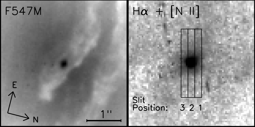
Figure 1.— HST WFPC2/PC F547M (left) and continuum-subtracted H$\alpha$+[N II] (right) images of the M84 nucleus. STIS observations were made at the three adjacent slit positions shown by the rectangular regions overplotted on the continuum-subtracted image. The length of the rectangular regions corresponds to the region over which we could measure the emission lines. Both images have been rotated such that the STIS instrumental $y$-axis points upward. Each box is 3$\farcs$7 on a side.

We also obtained Wide Field Planetary Camera 2 (WFPC2) F547M, F658N, and F814W images from the HST archive, originally observed under program GO-6094. In each image, the nucleus was centered on the PC detector. The images for each of the filters were taken as a sequence of two individual exposures, and we used the IRAF combine task to average the exposures together and reject cosmic rays. However, a number of cosmic rays remained even after using the combine task, and so we applied an extra cosmic ray cleaning step to the combined image using the LA-COSMIC task (van Dokkum, 2001). The total exposure times were 1200 s, 2600 s, and 520 s for the F547M, F658N, and F814W images, respectively.

We created a continuum-subtracted H$\alpha$+[N II] image by subtracting a scaled combination of the F547M and F814W images from the F658N image. We experimented with different scaling factors, and searched for a set of factors that would produce a background region in the continuum-subtracted image with a mean flux as close to zero as possible. In Figure 1, we show the continuum-subtracted image with the location of the STIS slits overlaid, as well as the F547M WFPC2 image. As previously described by Bower et al. (1997), the emission-line image reveals a compact central source surrounded by an extended disk-like structure that traces the nuclear dust disk.

3. Measurement of Emission Lines

We extracted spectra from individual rows of the 2D STIS image out to about 0$\farcs$85 from the slit center. The rows were extracted as far out as the emission lines were detectable. Far from the slit center, where the emission lines were weak, we binned together multiple rows to improve the S/N. Before fitting the emission lines, we removed the continuum from the spectrum. For each row, we fit a line to the continuum regions between rest-wavelengths $6500$–$6650$ Å and $6700$–$6750$ Å, and then subtracted the continuum fit from the spectrum. Generally, a straight line is not a good description of the continuum near H$\alpha$, but with the low S/N in the continuum at most positions and the small wavelength range, we could not perform a more accurate subtraction.

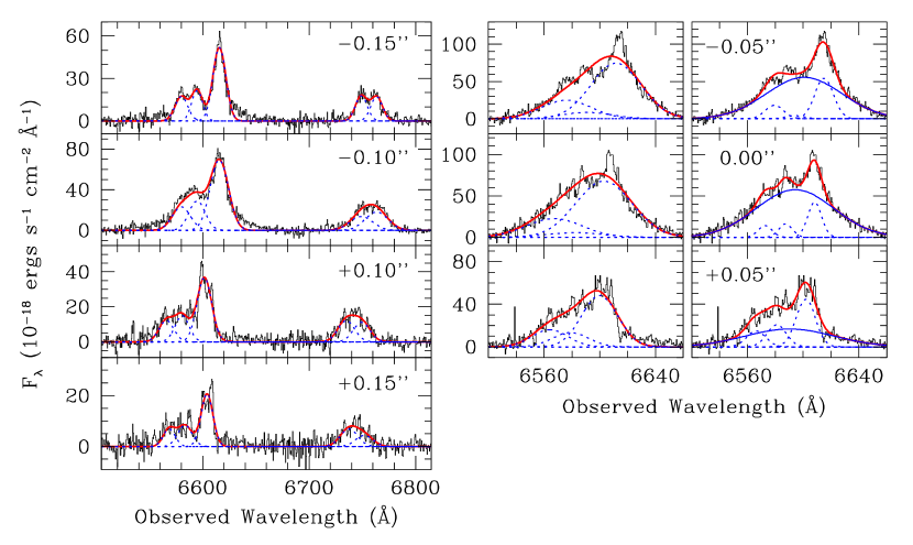
Figure 2.— Spectra extracted from the central slit located within 0$\farcs$15 from the M84 nucleus. For the spectra located at $\pm$0$\farcs$1 and $\pm$0$\farcs$15 from the nucleus (left), each emission line was fit with a single Gaussian according to the basic model described in §3. For the spectra extracted from the three innermost rows (right), we show the fit results from the basic model with an additional constraint on the H$\alpha$ and [N II] line widths, and the same model but with a single Gaussian broad component (shown by the blue solid line). In all panels, the single Gaussian narrow components are shown by blue dashed lines and the sum of all the Gaussian components are given by the red solid line.

We applied a Levenberg-Marquardt least-squares minimization technique using the MPFIT library in IDL (Markwardt, 2009) in order to fit each spectrum with a set of Gaussians, following the same technique described by Walsh et al. (2008). We used the propagated error spectra to weight the data points during the fit. For all but the three innermost rows of the central slit, we simultaneously fit five Gaussians to the H$\alpha$, [N II] $\lambda\lambda 6548,6583$, and [S II] $\lambda\lambda 6716,6731$ emission lines. All the lines were required to have a common velocity, and the fluxes of the [N II] lines were held at a $3:1$ ratio. The widths of the [N II] lines were required to be the same. Also, the [S II] lines were constrained to have equal velocity widths.

Spectra extracted from the central slit position at 0$\farcs$15 and 0$\farcs$10 from the nucleus clearly exhibit double-peaked line profiles. Our basic model described previously provides a good fit to the spectra at 0$\farcs$15 and 0$\farcs$10, but we also tried fitting two Gaussians to each emission line (representing two kinematically distinct gas components). While the two-component model fits the spectra very well at these locations, the $\chi^{2}$ per degree of freedom ($\chi^{2}_{\nu}$) decreased by less than 12% compared to the basic model.

The basic model, however, did not return adequate fits for the spectra extracted from the innermost three rows of the central slit position, which have a very complex, asymmetric shape with severely blended H$\alpha$ and [N II] lines that may be double-peaked. We then applied an additional constraint to the basic model that required the widths of the H$\alpha$ and [N II] lines to be equal. Even with this model, the fit was poor and it was impossible to obtain accurate and unique mean velocities, velocity dispersions, or fluxes. The velocity dispersion values were very large, ranging from $\sim 600$ – 900 km s^-1, and the best-fit Gaussian appeared to be systematically shifted blueward of the peak [N II] $\lambda 6583$ flux in all three rows. We also tried fitting a number of more complicated models, such as adding a single Gaussian broad component to the H$\alpha$ + [N II] complex or fitting a two-component model. These more complex, multi-component fits were not well constrained by the data, often resulting in Gaussian components with zero flux. Moreover, including a broad component in the fit usually resulted in unreasonably small fluxes and line widths for the H$\alpha$ and [N II] narrow components, although these models did seem to provide a better estimate of the mean velocity than the previous fitting attempts.

Past work by Bower et al. (1998) has interpreted these complex line profiles as arising from two separate gas components. They fit two Gaussian components at number of locations within 0$\farcs$3 from the nucleus, and only used one of the two components in order to derive a black hole mass. However, as described above, modeling by Maciejewski & Binney (2001) and Barth et al. (2001b) has shown that the line profiles can be described by a rotating disk model rather than requiring two dynamically distinct components. Our detailed modeling further supports this interpretation and will be discussed in §6. Thus, for the spectra located at 0$\farcs$15 and 0$\farcs$10, we use the fit results from the basic model, with one Gaussian component for each narrow emission line.

In the three innermost CCD rows of the central slit position, the complexity and blending of the line profiles prevents an accurate decomposition into Gaussian components, and it is not clear whether a broad H$\alpha$ component is even present. The broad wings on the H$\alpha$+[N II] complex could plausibly result from either a compact broad-line region, or from the rapid rotation of the innermost, unresolved portion of the emission-line disk, or both. Thus, we consider all measurements from these central three rows to be unreliable, and we do not use them to constrain our dynamical models. Since the line profiles in these central three rows are dominated by PSF blurring and rotational broadening, they add relatively little useful information to constrain the disk models, and we will show in §6 that the modeling results are insensitive to the values of the observed velocity from these central three STIS rows. However, for reference in the remaining figures presented in the paper, we continue to plot the mean velocity (measured from a fit using the basic model along with a single Gaussian broad component and a constraint requiring the widths of the narrow H$\alpha$ and [N II] lines to be equal). We do not show the velocity dispersion or flux measurements from the central three rows in these figures though because we were unable to obtain reasonable measurements from any of our fitting attempts.

In Figure 2, we show a few examples of the basic model fit to the spectra extracted from the central slit position at $\pm$0$\farcs$1 and $\pm$0$\farcs$15 from the nucleus. We also display the fits to the spectra from the innermost three rows using the basic model plus an additional line width constraint, as well as the basic model along with a single Gaussian broad component and a line width constraint on the H$\alpha$ and [N II] narrow components.

In order to estimate the uncertainties on the free parameters, we used a Monte Carlo technique. For each row, we generated new spectra by adding random Gaussian noise to the original spectrum, where the 1$\sigma$ level of the perturbation was set by the residuals between the best-fit model and the original spectrum. The new spectra were then refit, and the 1$\sigma$ uncertainties were taken to be the standard deviation of the distribution. This method resulted in velocity and velocity dispersion errors that were typically 27% and 40% larger, respectively, than the formal uncertainties from the best-fit model.

4. The Observed Velocity Field

From the fits to the [N II] $\lambda 6583$ emission line, we obtained the velocity, velocity dispersion, and flux, and we plot these values as a function of position along the slit in Figure 3. We defined the galaxy center (Y-Offset = 0″) to be the row with the largest continuum flux, which also coincided with the peak of the narrow [N II] $\lambda 6583$ emission-line flux. The grey open squares mark the three central rows where the complex line profiles precluded any definitive measurements of the [N II] mean velocity, velocity dispersion, or flux. These grey points mark the velocity of the [N II] emission peak as determined by the fits that included a broad H$\alpha$ component. For reference, we also show the best-fit systemic velocity determined from our gas-dynamical modeling.

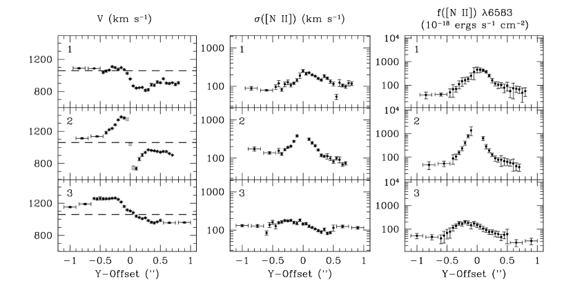
Figure 3.— The velocity, velocity dispersion, and flux measured from the [N II] $\lambda 6583$ emission line as a function of location along each of the three slit positions in M84. The grey open squares mark the velocity measurements from the three central rows where we had difficulty fitting the spectra, while the unreliable velocity dispersion and flux measurements from the three innermost rows are left off the figure. The numbers at the top left of each plot correspond to the slit locations depicted in Figure 1. The positive and negative Y-Offsets correspond to spectra extracted from the rows above and the rows below the central row, respectively, when the slits are oriented such that the STIS instrumental y-axis points upward. Thus, the bottom half of the slit drawn in Figure 1 corresponds to negative Y-Offsets and the top half of the slit in Figure 1 corresponds to positive Y-Offsets. Spectral rows that were binned together in order to improve the S/N are shown with error bars in the Y-Offset direction. For reference, the dashed line shows the best-fit systemic velocity determined from our gas-dynamical modeling.

The multi-slit velocity curves show the gas participates in regular rotation. There is a steep velocity gradient across the inner 0$\farcs$2 of slit position 2, where the radial velocity drops from 1380 km s^-1 at Y-offset = $-$0$\farcs$1 to 740 km s^-1 at Y-offset = 0$\farcs$1. The radial velocities measured from slit position 3 show that the gas located to the southwest of the nucleus is mostly redshifted relative to the galaxy’s systemic velocity, while the data from slit position 1 show that the gas to the northeast of the nucleus is mostly blueshifted. The [N II] $\lambda 6583$ line widths measured from the central slit position are large, with velocity dispersions of $\sim 400$ km s^-1 and $\sim 300$ km s^-1 at Y-offset = $-$0$\farcs$1 and 0$\farcs$1, respectively. The line widths continue to rise toward the nucleus. However, due to the complexity of the spectra, which are severely blended together due to the large rotational broadening and the PSF blurring, we were unable to obtain reliable measurements of the velocity, velocity dispersion, or flux from the innermost three STIS rows.

5. Modeling the Velocity Field

The velocity field was modeled assuming that the gas is in circular rotation in a thin disk-like structure. We follow a method similar to that outlined by Barth et al. (2001), and we refer the reader there for a more detailed discussion of the model. At each radius $r$ in the disk, we determine the circular velocity relative to the systemic velocity ($v_{\mathrm{sys}}$), based on the enclosed mass $M(r)$, which depends on the black hole mass ($M_{\mathrm{BH}}$), the stellar mass profile, and the stellar mass-to-light ratio ($\Upsilon$). The stellar contribution to the circular velocities will be discussed in §5.1.

We then project the disk velocity field onto the plane of the sky for a given value of the disk inclination $i$ in order to determine the line-of-sight projection of the rotation velocity at each position in the inclined disk. We generated the model velocity field on a highly subsampled pixel grid; each model pixel was 10$\times$ oversampled relative to the STIS pixel size. Previous studies have used smaller subsampling factors of $s=2$ and $s=4$ (Barth et al., 2001; Coccato et al., 2006; Wold et al., 2006). However, we found that a large subsampling factor was necessary in order to sufficiently capture the considerable changes in velocity that occur over small spatial scales near the M84 nucleus, and to more accurately model the steep emission-line flux profile. We experimented with a range of subsampling factors ($s$), which will be discussed further in §6, before settling on a subsampling factor of $s=10$.

We calculate the intrinsic line-of-sight velocity profiles on a velocity grid with a bin size that matches the STIS pixel scale of 25.2 km s^-1. The intrinsic line-of-sight velocity profiles are assumed to be Gaussian before passing through the telescope optics. The Gaussian profiles are centered on the projected line-of-sight velocity at each point on the model grid. Furthermore, the line-of-sight velocity profiles are weighted by the emission-line flux distribution (to be discussed in §5.2). The width of the intrinsic line-of-sight velocity profiles (to be discussed in §5.3) includes contributions from the thermal velocity dispersion of the gas, the instrumental line spread function (LSF) for STIS, and an intrinsic turbulent velocity dispersion.

The model velocity field is then synthetically “observed” in a manner that matches the STIS observations. This synthetic observation includes accounting for the blurring by the telescope PSF. We used Tiny Tim (Krist & Hook, 2004) to create a 10$\times$ oversampled 0$\farcs$3$\times$0$\farcs$3 portion of the full STIS PSF for a monochromatic filter passband at 6600 Å. Although a 0$\farcs$3-diameter PSF model excludes part of the STIS PSF wings, there is a negligible effect on the inferred black hole mass, as will be demonstrated in §6. Each velocity slice of the line profile grid is then convolved with the oversampled 0$\farcs$3$\times$0$\farcs$3 Tiny Tim PSF model.

After accounting for the telescope PSF, we propagate the model velocity field through the STIS slit. The STIS slit is allowed to lie at some angle $\theta$ from the projected major axis of the gas disk, and the slit can be displaced some distance along the slit width ($x_{\mathrm{offset}}$) and along the slit length ($y_{\mathrm{offset}}$) from the black hole. We included the shifts in velocity that arise as a result of the finite slit width. The velocity shifts occur because a photon’s recorded wavelength depends on the location along the slit width at which the photon enters (e.g., Barth et al., 2001; Maciejewski & Binney, 2001).

After the velocity shifts have been made, we rebin the resulting emission-line profiles to the STIS pixel size. Thus, we are left with a model 2D spectral image similar to the STIS data. We convolve the model 2D spectral image with the CCD charge diffusion kernel. The CCD charge diffusion kernel is given by Tiny Tim for model PSFs that are subsampled, and it represents the charge that is spread between the immediate neighboring (non-subsampled) pixels.

Finally, spectra are extracted on a row-by-row basis from the model STIS 2D image. We fit a single Gaussian to the emission line, analogous to the measurements of the emission lines from the STIS data. We are thus able to measure the model velocity, velocity dispersion, and flux as a function of position along the slit. We then determine the best-fit model parameters ($M_{\mathrm{BH}}$, $\Upsilon$, $i$, $v_{\mathrm{sys}}$, $\theta$, $x_{\mathrm{offset}}$, $y_{\mathrm{offset}}$) that produce a model velocity field that most closely matches the observed velocity field over a region ($r_{\mathrm{fit}}$) that extends from $-$0$\farcs$5 to 0$\farcs$5 for each slit position. However, we do not include the uncertain velocity measurements from the innermost three STIS rows in the fit. We measure the black hole mass and the $\chi^{2}$ from the model fits to the observed velocity only, after separately optimizing the model fits to the observed line widths and fluxes as described below. The observed [N II] line widths and fluxes are not directly dependent on the black hole mass, so the black hole mass is determined from the fit to just the radial velocity curves.

5.1. Stellar Mass Profile

In order to account for the stellar contribution to the gravitational potential, we modeled the intrinsic density distribution of the central regions of M84 as the sum of spherically symmetric components with Gaussian profiles, as done by Sarzi et al. (2001), Barth et al. (2001), Sarzi et al. (2002), and Coccato et al. (2006). Within such a multi-Gaussian framework (Monnet, Bacon, & Emsellem, 1992), projecting the model density profile on the sky to match the observed surface brightness is fairly simple given the properties of the Gaussian function. This is particularly true when the instrumental PSF is also expressed in terms of Gaussian functions. Once the (non-negative) amplitudes of the Gaussian density components have been determined, the contribution of each Gaussian to the stellar potential can be conveniently evaluated in terms of error functions.

For M84, we deprojected the $V$-band surface brightness profile of Kormendy et al. (2009), who combined large scale ground-based images with high-resolution HST NICMOS $H$-band data for the central, dusty region. Since the NICMOS PSF is fairly complex, we took particular care to describe it in terms of Gaussian components by matching to a NIC2 F205W PSF generated with Tiny Tim. A careful representation of the PSF is important in the presence of an active nucleus, as in the case of M84, because it affects the isolation and removal of an AGN component from the stellar mass budget.

The luminosity profile of M84 contains a compact central component. Bower et al. (2000) show that this central component is due to the AGN itself and not a nuclear star cluster, so the light from this component should not contribute to the stellar mass profile. In order to determine the impact of this component on the mass models, we computed two different deprojected stellar mass profiles, one in which this central component was assumed to be AGN light, and another in which it was assumed to be starlight with the same stellar mass-to-light ratio as the rest of the galaxy.

In Figure 4, we present the final product of the multi-Gaussian deprojection of the surface-brightness profile of M84, that is, the stellar contribution to the circular velocity in the galaxy. The circular velocity due to a $4\times 10^{8}$ $M_{\odot}$ black hole is also illustrated, since this is a plausible lower limit to the black hole mass based on our results and those of Maciejewski & Binney (2001). The figure illustrates that the stellar contribution to the circular velocities is extremely small over the radial range probed by our data ($\sim 0\farcs 5$), even for the lowest reasonable value of $M_{\rm BH}$. The stellar contribution is negligibly small regardless of whether the central compact component in the light profile is assumed to be a star cluster or an AGN.

The results shown in Figure 4 indicate that the total mass within the inner 0$\farcs$5 is likely to be dominated by the black hole. In other words, the black hole’s dynamical sphere of influence is extremely well resolved by the STIS observations; this is consistent with the nearly Keplerian shape of the velocity profile along the central slit position. As a result, our model fits should be fairly insensitive to the stellar mass-to-light ratio $\Upsilon$. In fact, as we describe below, our dynamical models do not provide any useful constraints on $\Upsilon$, and we simply assume a fixed value of $\Upsilon$ for our final model fits. In our dynamical models, we used the circular velocities derived under the assumption that the central compact component represents AGN light.

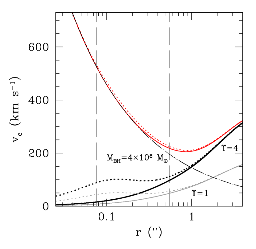
Figure 4.— Stellar contribution to the circular velocity ($v_{c}$) obtained from the multi-Gaussian deprojection of the M84 $V$-band surface brightness profile. The thick black and thin grey radially increasing lines show $v_{c}$ values obtained assuming stellar mass-to-light ratios of $\Upsilon=4$ and $1$, respectively. Two different stellar $v_{c}$ values are shown; the solid curves illustrate the case where the central compact source in the light profile is assumed to be the AGN (in which case it makes no contribution to the stellar mass profile), while the dotted curves illustrate the case in which it is assumed to be a compact stellar nucleus. The black dot-dashed line shows the Keplerian velocities produced by a $4\times 10^{8}\ M_{\odot}$ black hole, which, when added to the stellar potential obtained with $\Upsilon=4$, would lead to the red solid and dotted lines that trace a nearly parabolic trend. Over the radial range we fit the kinematic data (shown by the vertical grey dashed lines, see §6), $v_{c}$ is almost entirely determined by the black hole mass. Whether the light from the central compact component is excluded or included in the mass budget does not significantly alter the estimate of $M_{\rm BH}$.

5.2. Emission-Line Flux

As discussed above in §5, the model line-of-sight velocity profiles are weighted by the emission-line flux at each point in the disk. Past gas-dynamical models have used either an analytic form to describe the intrinsic emission-line flux (e.g., Verdoes Kleijn et al., 2002; Coccato et al., 2006; Marconi et al., 2006; Pastorini et al., 2007; Hicks & Malkan, 2008) or the continuum-subtracted H$\alpha$ + [N II] image directly, after deconvolution with the telescope PSF (e.g., Barth et al., 2001; Shapiro et al., 2006; Wold et al., 2006; Dalla Bontà et al., 2009). Barth et al. (2001) found that folding the deconvolved continuum-subtracted image into the model calculations can account for small-scale irregularities in the velocity field. However, our attempts to use a deconvolved image of M84 were unsuccessful, and the dynamical model produced poor fits to both the observed flux and velocity. It appeared that the deconvolved continuum-subtracted image could not adequately characterize the steepness of the nuclear emission-line light on subpixel scales.

We therefore experimented with analytic forms of various complexity for the intrinsic flux distribution. We searched for the simplest function that would sufficiently reproduce the observed [N II] flux profile while simultaneously producing model velocities closest to the observed velocities. We tested parametrizations that were composed of two to four components, and the components were either Gaussian functions [parametrized as $F(r)=F_{0}\exp(-r^{2}/2r_{s}^{2})$], exponential functions [parametrized as $F(r)=F_{0}\exp(-r/r_{s})$], or constants. We experimented with models representing intrinsically circularly symmetric disks (producing concentric elliptical isophotes with constant position angle and axis ratio), as well as more complicated models where the isophotes of the individual components were allowed to have different centers, positions angles, and axis ratios. The parameters for each possible surface brightness model were determined by computing disk models including the parametrized surface brightness model, calculating the resulting model line profiles as described above in §5, measuring the emission-line fluxes in the resulting model, and then optimizing the fit of the modeled fluxes to the observed [N II] flux distribution by minimizing $\chi^{2}$. Ultimately, we found that the best parametrization was the sum of four components: three concentric Gaussians describing the compact nucleus, plus a more extended exponential component with an offset center relative to the positions of the Gaussian components. The amplitudes ($F_{0}$), scale radii ($r_{s}$) along the major axis, position angles, axis ratios ($b/a$), and centroid positions for each of these elliptical components in the best-fitting model are listed in Table 1.

Table 1Emission-Line Flux Parameters

Component	$F_{0}$	$r_{s}$	$x_{\mathrm{cen}}$	$y_{\mathrm{cen}}$	PA	$b/a$
		(pc)	(″)	(″)	(∘)
Gaussian	234.2	0.5	0.00	0.00	344	0.9
Gaussian	126.6	2.8	0.00	0.00	33	0.4
Gaussian	6.0	12.0	0.00	0.00	31	0.4
Exponential	1.0	50.0	0.13	0.02	69	0.7

Note. — The amplitude, $F$, is in arbitrary flux units. The center of the ellipse is described by $x_{\mathrm{cen}}$ and $y_{\mathrm{cen}}$, relative to the location of the black hole. The position angle, PA, is in units of degrees clockwise, with PA $=0$ pointing along the length of the STIS slit.

5.3. Line Widths

A number of factors contribute to the width of the line-of-sight velocity profiles, such as rotational broadening, instrumental broadening, thermal broadening, and possibly an intrinsic velocity dispersion in the gaseous disk. Rotational broadening occurs because light from different parts of the disk falls within the same slit and consequently is blended together. Instrumental broadening includes the PSF blurring, the velocity shifts that occur as a result of the finite slit width, and the effects of charge diffusion between neighboring pixels. All of these instrumental effects, as well as the rotational broadening, are explicitly included in our modeling when the intrinsic line-of-sight velocity profiles are propagated through the telescope and spectrograph. Before the line-of-sight velocity profiles are propagated through the telescope optics, we assign the line profiles a small width resulting from the intrinsic instrumental line-spread function estimated by Barth et al. (2001) to be $\sigma_{\mathrm{LSF}}=8$ km s^-1 and a velocity dispersion of $\sigma_{\mathrm{th}}=10$ km s^-1, which is the expected thermal contribution to the line width for gas with a temperature of $\approx 10^{4}$ K. Since the values of $\sigma_{\mathrm{LSF}}$ and $\sigma_{\mathrm{th}}$ are very small compared with the observed line widths, they have a negligible effect on the model calculation.

Even though the models accounted for the rotational, instrumental, and thermal broadening, our preliminary models predicted line widths that were much smaller than the observed velocity dispersions in M84. This behavior has often been seen in past studies of other galaxies (e.g., van der Marel & van den Bosch, 1998; Verdoes Kleijn et al., 2000, 2002; Shapiro et al., 2006; Dalla Bontà et al., 2009). However, previous work has also found that rotational and instrumental broadening alone can explain the observed line widths in some objects (e.g., Macchetto et al. 1997; Capetti et al. 2005; Atkinson et al. 2005; de Francesco et al. 2006, 2008). In order to produce model line widths that match the observations, we include a projected intrinsic velocity dispersion of the form

$$\sigma_{\mathrm{p}}=\sigma_{0}+\sigma_{1}\exp{\bigg{(}\frac{-r}{r_{0}}\bigg{)}}\;.$$ (1)

Thus, the width of the line-of-sight velocity profiles is given by $\sigma_{\mathrm{th}}$, $\sigma_{\mathrm{LSF}}$, and $\sigma_{\mathrm{p}}$ added in quadrature, combined with the width resulting from the propagation of the line profiles through the telescope and spectrograph. We determined that $\sigma_{0}=77$ km s^-1, $\sigma_{1}=214$ km s^-1, and $r_{0}=26$ pc by fitting the line widths predicted from a preliminary model to the observed line widths. The unreliable velocity dispersion measurements from the three central STIS rows were excluded from the fit.

The physical nature of the intrinsic velocity dispersion is not understood. van der Marel & van den Bosch (1998) proposed that the intrinsic velocity dispersion is the result of local microturbulence, but that the bulk motion of the gas remains in circular motion. Others suggest the local random motions may contribute pressure support to the disk, which if ignored will lead to an underestimate of the black hole mass (e.g., Barth et al., 2001; Neumayer et al., 2007). Verdoes Kleijn, van der Marel, & Noel-Storr (2006) find that radio galaxies in particular (including M84) often show evidence for nuclear velocity dispersions in excess of those expected from pure gravitational motions. They attribute the excess velocity dispersion to non-gravitational motions in the gas.

While there remains no current clear consensus as to the physical mechanism that causes the discrepancy between the model line widths and the observed velocity dispersions, we examine two scenarios that should cover the possible range of masses for the black hole in M84. First, we consider the case in which the intrinsic velocity dispersion does not affect the circular velocity. Secondly, we analyze the case in which the intrinsic velocity dispersion contributes dynamical support to the disk, and we apply an asymmetric drift correction.

5.4. Asymmetric Drift Correction

If the intrinsic velocity dispersion provides pressure support that balances gravity in the gas disk, then the observed mean rotation speed ($v_{\phi}$) will be smaller than the local circular velocity ($v_{c}$) for a given black hole mass. Models that do not account for this effect will lead to black hole mass measurements that underestimate the true mass. Although it is unclear whether the intrinsic velocity dispersion actually does provide dynamical support to the disk, we include an asymmetric drift correction in our model to estimate an upper limit to the M84 black hole mass, following the methods previously described by Barth et al. (2001).

Briefly, if we assume that the gas motions are isotropic in the $r$ and $z$ (cylindrical) coordinates, then asymmetric drift correction is given by

$$v_{c}^{2}\ -\ v_{\phi}^{2}\ =\ \sigma_{r}^{2}\bigg{[}-\frac{d\ln\nu}{d\ln r}\ -\ \frac{d\ln\sigma_{r}^{2}}{d\ln r}\ -\ \bigg{(}1\ -\ \frac{\sigma_{\phi}^{2}}{\sigma_{r}^{2}}\bigg{)}\bigg{]}\;.$$ (2)

Here, $\nu$ is the number density of tracer particles or clouds in the gaseous disk, and we assume that intrinsic radial velocity dispersion $\sigma_{r}$ can be described by an exponential + constant of the same form as Equation 1. For a given parametrization of $\sigma_{r}$, we determine $\sigma_{\phi}$ and the projected velocity dispersion following the method described by Barth et al. (2001). This projected velocity dispersion is then added in quadrature to $\sigma_{\mathrm{th}}$ and $\sigma_{\mathrm{LSF}}$ (discussed in §5.3) in order to obtain the widths of the line-of-sight velocity profiles before propagation through the telescope and spectrograph. We found best-fit values of $\sigma_{0}=37$ km s^-1, $\sigma_{1}=255$ km s^-1, and $r_{0}=53$ pc by computing preliminary disk models with an asymmetric drift correction and fitting the model line widths to the observed [N II] line widths. A similar expression for the asymmetric drift correction is given by Valenzuela et al. (2007), including an additional term that accounts for the effect of gas pressure gradients. We neglect this additional term as it provides only a small contribution to the asymmetric drift correction.

6. Modeling Results

In order to determine the best-fit model parameters ($M_{\mathrm{BH}}$, $\Upsilon$, $i$, $v_{\mathrm{sys}}$, $\theta$, $x_{\mathrm{offset}}$, $y_{\mathrm{offset}}$), we minimized $\chi^{2}$ using the downhill simplex algorithm by Press et al. (1992). Initially, we ran preliminary models without an asymmetric drift correction allowing all seven model parameters to vary independently. However, it became clear that the stellar mass-to-light ratio could not be well constrained by the STIS data. The black hole’s sphere of influence is so well resolved that we are unable to determine a precise value for $\Upsilon$. Our preliminary models often returned unreasonably low values of $\Upsilon=0$. Therefore, we estimated $\Upsilon$ based on the $B-V$ color for the galaxy using Bell et al. (2003). The $B-V$ color from the Third Reference Catalogue of Bright Galaxies (RC3) (de Vaucouleurs et al., 1991) is 0.98, which implies $\Upsilon\sim 4$ in $V$-band solar units. We then fixed $\Upsilon$ to this value in our models.

We also calculated preliminary models using different PSF sizes, subsampling factors, and fitting regions. During all of these model calculations, the parameters $M_{\mathrm{BH}}$, $i$, $\theta$, $v_{\mathrm{sys}}$, $x_{\mathrm{offset}}$, and $y_{\mathrm{offset}}$ were allowed to vary during the fit, but $\Upsilon$ was fixed at 4 in $V$-band solar units. Also, the uncertain velocity measurements from the three central STIS rows were excluded from the fit. In Figure 5, we present the results of the models without an asymmetric drift correction.

Figure 5.— Black hole mass as a function of PSF size (with $s=10$ and $r_{\mathrm{fit}}=$ 0$\farcs$5), subsampling factor (with a 0$\farcs$3-diameter PSF and $r_{\mathrm{fit}}=$ 0$\farcs$5), and fitting radius (with a 0$\farcs$3-diameter PSF and $s=10$), respectively. The quantities $M_{\mathrm{BH}}$, $i$, $\theta$, $v_{\mathrm{sys}}$, $x_{\mathrm{offset}}$, and $y_{\mathrm{offset}}$ were allowed to vary during the fit, but $\Upsilon$ was fixed at 4 $V$-band solar units. All models were calculated without an asymmetric drift correction.

In order to test the significance of the PSF size on the black hole mass measurement, we calculated disk models using Tiny Tim PSFs ranging in size from 0$\farcs$3 to 0$\farcs$6 in diameter. All of these model PSFs exclude part of the extended STIS PSF wings, with the omitted flux totaling 18%, 13%, 11%, and 9% of the entire PSF flux for a 0$\farcs$3, 0$\farcs$4, 0$\farcs$5, and 0$\farcs$6-diameter PSF, respectively. We found that the PSF size has a small impact on the black hole mass measurement, with $M_{\mathrm{BH}}$ varying between $4.3\times 10^{8}\ M_{\odot}$ and $4.5\times 10^{8}\ M_{\odot}$ for the models without an asymmetric drift correction. Because the computation time increases rapidly with PSF size, and the PSF size has a minimal impact on the black hole mass, we used the Tiny Tim 0$\farcs$3-diameter PSF in our final models.

When testing the effect of the subsampling factor on the black hole mass, we calculated disk models using using subsampling factors between $s=2$ and $s=10$ in increments of two. We found that the black hole mass did not vary significantly with the subsampling factor. For models without an asymmetric drift correction, $M_{\mathrm{BH}}$ fluctuated between $4.1\times 10^{8}\ M_{\odot}$ and $4.3\times 10^{8}\ M_{\odot}$. Although the black hole mass was almost unaffected by the subsampling factor, we found that larger subsampling factors resulted in much better fits to both the emission-line flux and velocities. Small subsampling factors were unable to capture the large changes in both the velocity and emission-line flux seen near the M84 nucleus. Thus, in our final models we used $s=10$.

Similarly, we calculated disk models with $r_{\mathrm{fit}}$ values between 0$\farcs$3 and 1″. Like with the PSF and subsampling factor, the size of the fitting region had a small impact on the black hole mass, with $M_{\mathrm{BH}}$ between $4.2\times 10^{8}\ M_{\odot}$ and $4.5\times 10^{8}\ M_{\odot}$ for the models without an asymmetric drift correction. Using the largest possible fitting region is not necessarily the best approach because there can be systematic departures from the disk model at large radii, possibly due to disk warping. The region in the central slit position near Y-Offset$=-0\farcs 5$, in particular, is not well fit by any of the disk models. We used $r_{\mathrm{fit}}=$ 0$\farcs$5 in our final models because this region is large enough to contain an adequate number of velocity measurements needed to constrain the model, but also small enough so that the disk model still provides a good description of the observations.

We also experimented with using different analytic parametrizations of the intrinsic emission-line flux distribution. In Figure 6, we present the results of disk models without an asymmetric drift correction, in which the emission-line flux was modeled with three additional functions of varying complexity: 1 Gaussian $+$ 1 exponential (model B), 2 exponentials (model C), and 2 Gaussians $+$ 1 exponential (model D). The isophotes of the components in models B, C, and D are elliptical and have different centers, position angles, and axis ratios similar to the emission-line flux distribution composed of 3 Gaussians $+$ 1 exponential adopted for the final model (model A) discussed in §5.2.

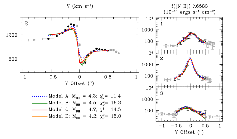
Figure 6.— Results of disk models with four different parametrizations of the emission-line flux: 3 Gaussians $+$ 1 exponential (model A), 1 Gaussian $+$ 1 exponential (model B), 2 exponentials (model C), and 2 Gaussians $+$ 1 exponential (model D). We present the model velocity for the central slit position (left) and the model emission-line flux from all three slit positions (right), as well as the best-fit $M_{\mathrm{BH}}$ in units of $10^{8}\ M_{\odot}$ and the corresponding $\chi^{2}_{\nu}$. All models were calculated without an asymmetric drift correction using a 0$\farcs$3-diameter PSF and $s=10$. The fitting radius was set to $r_{\mathrm{fit}}=$ 0$\farcs$5, and thus the black filled circles are the data measured from the STIS observations that were included in the fit while the grey open squares are the data that were excluded. The quantities $M_{\mathrm{BH}}$, $i$, $\theta$, $v_{\mathrm{sys}}$, $x_{\mathrm{offset}}$, and $y_{\mathrm{offset}}$ were allowed to vary during the fit.

Models A, B, C, and D reproduced the observed emission-line flux within the errors, but the quality of the fit to the observed velocity varied significantly ($\chi^{2}_{\nu}$ ranged from 11.4 – 16.3 for the models without an asymmetric drift correction). Although the intrinsic emission-line flux distribution affected the quality of the velocity fit, it only had a small influence on $M_{\mathrm{BH}}$, with the best-fit mass between $4.2\times 10^{8}\ M_{\odot}$ and $4.7\times 10^{8}\ M_{\odot}$. The observed emission-line flux could also be fit with two additional analytic functions: 3 exponentials and 3 Gaussians $+$ 1 exponential with a nuclear hole. When optimizing this last model to the observed flux distribution, we found a best-fit hole radius of 0.8 pc, which is well within a single STIS pixel. The emission-line flux models composed of 3 exponentials and 3 Gaussians $+$ 1 exponential with a nuclear hole produced a black hole mass of $4.5\times 10^{8}\ M_{\odot}$ and a $\chi^{2}_{\nu}$ of 13.7 and 12.3, respectively. These two models are left off Figure 6 for clarity, but similarly show that the black hole mass does not change drastically. Our findings are consistent with Marconi et al. (2006), who demonstrated that the emission-line flux model has little effect on the final black hole mass measurement for Centaurus A. Many other emission-line flux models were tested, but the models returned unacceptable fits to the observed flux, and thus they are not presented here.

The other disk parameters appeared to be well constrained by the multi-slit STIS data. Throughout the numerous calculations of preliminary models without an asymmetric drift correction, the parameters $i$, $v_{\mathrm{sys}}$, $\theta$, $x_{\mathrm{offset}}$, and $y_{\mathrm{offset}}$ varied at most by 8^∘, 10 km s^-1, 6^∘, 0$\farcs$03, and 0$\farcs$03, respectively. Similarly, we found deviations of at most 10^∘, 12 km s^-1, 8^∘, 0$\farcs$03, and 0$\farcs$04 for $i$, $v_{\mathrm{sys}}$, $\theta$, $x_{\mathrm{offset}}$, and $y_{\mathrm{offset}}$, respectively, for the models with an asymmetric drift correction. The uncertainty in the black hole mass due to these parameters is negligible, but will be accounted for in §6.3 when the formal model fitting uncertainty is determined.

6.1. Models Without an Asymmetric Drift Correction

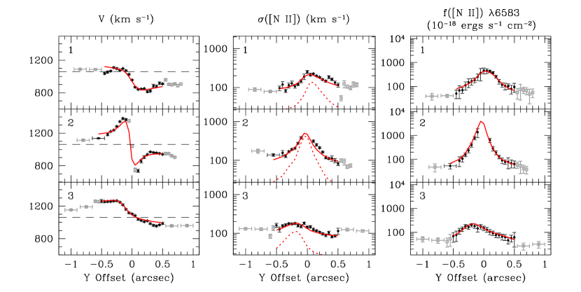
Figure 7.— Results of the final model without an asymmetric drift correction using a 0$\farcs$3-diameter PSF, $s=10$, and $r_{\mathrm{fit}}=$ 0$\farcs$5. The model velocity, velocity dispersion, and emission-line flux are shown by the red solid line. The red dotted line shows the model velocity dispersion if an intrinsic velocity dispersion is not included in the model. We applied a single scaling factor to the model emission-line flux such that the median values of the model and the data would match. The black filled circles are the data from the STIS observations that were included in the fit, while the grey open squares are the data that were excluded from the fit. For reference, the horizontal dashed line shows the best-fit systemic velocity determined from the final model.

The final model without an asymmetric drift correction was calculated using a 0$\farcs$3 $\times$ 0$\farcs$3 PSF, a subsampling factor of $s=10$, and a fitting region of $r_{\mathrm{fit}}=$ 0$\farcs$5. Due to the complexity of the spectra extracted from the three central STIS rows and the resulting uncertainty in the radial velocity measurements, we excluded these three innermost measurements from the final fit. The stellar mass-to-light ratio was fixed to a value of 4 in $V$-band solar units. We also included the projected intrinsic velocity dispersion described in §5.3.

In Figure 7 we compare the final model velocity, velocity dispersion, and emission-line flux to the observed values as a function of location along the slit for each of the three slit positions. As can be seen in this figure, the final model is able to sufficiently reproduce the shape of the observed velocity field and the emission-line flux. It is also apparent that an intrinsic velocity dispersion is needed in order to bring the model into agreement with the observations. In the left column of Table 2, we give the best-fit parameter values for the final model without an asymmetric drift correction.

Even though the final model matches the general shape of the velocity curves fairly well, we find that $\chi^{2}=594.7$. The 58 velocity measurements are fit with 6 parameters ($M_{\mathrm{BH}}$, $i$, $v_{\mathrm{sys}}$, $\theta$, $x_{\mathrm{offset}}$, and $y_{\mathrm{offset}}$), resulting in $\chi^{2}_{\nu}=11.4$. We acknowledge that our thin-disk model is unable to reproduce all of the velocity structure that is observed. As will be shown below in §6.3, removing several velocity measurements at locations that clearly deviate from pure circular rotation leaves the black hole mass unaffected while significantly improving $\chi^{2}_{\nu}$. Thus, we believe our $M_{\mathrm{BH}}$ measurement remains credible despite the moderate $\chi^{2}_{\nu}$ value. Furthermore, we account for the imperfect disk model in §6.3 by renormalizing $\chi^{2}_{\nu}$ before estimating the formal uncertainty in $M_{\mathrm{BH}}$ due to the model fitting process. We use this approach because it will provide the most conservative estimate of the uncertainty in the black hole mass. We note that several gas-dynamical models of other objects have similar $\chi^{2}_{\nu}$ values (e.g., Capetti et al., 2005; Atkinson et al., 2005; de Francesco et al., 2008; Dalla Bontà et al., 2009).

Table 2Final Disk Model Parameters

	w/o Asymmetric	w/ Asymmetric
	Drift	Drift
$M_{\mathrm{BH}}$ $(M_{\odot})$	(4.3${}^{+0.8}_{-0.7}$)$\times$108	(8.5${}^{+0.9}_{-0.8}$)$\times$108
$\Upsilon$ ($V$-band solar)	4	4
$i$ (∘)	67${}^{+1}_{-7}$	72${}^{+1}_{-9}$
$v_{\mathrm{sys}}$ (km s-1)	1060${}^{+6}_{-4}$	1060${}^{+9}_{-3}$
$\theta$ (∘)	27$\pm 3$	28${}^{+3}_{-5}$
$x_{\mathrm{offset}}$ (″)	0.02${}^{+0.02}_{-0.01}$	0.01${}^{+0.02}_{-0.01}$
$y_{\mathrm{offset}}$ (″)	$-$0.04${}^{+0.02}_{-0.01}$	$-$0.05${}^{+0.03}_{-0.01}$

Note. — Uncertainties given for the black hole mass are 68% confidence limits. The stellar mass-to-light ratio, $\Upsilon$, was frozen at 4 ($V$-band solar units) for both models. A relative angle of $\theta=27^{\circ}$ and $\theta=28^{\circ}$ corresponds to a disk major axis position angle of 77^∘ and 76^∘ east of north.

6.2. Models Including an Asymmetric Drift Correction

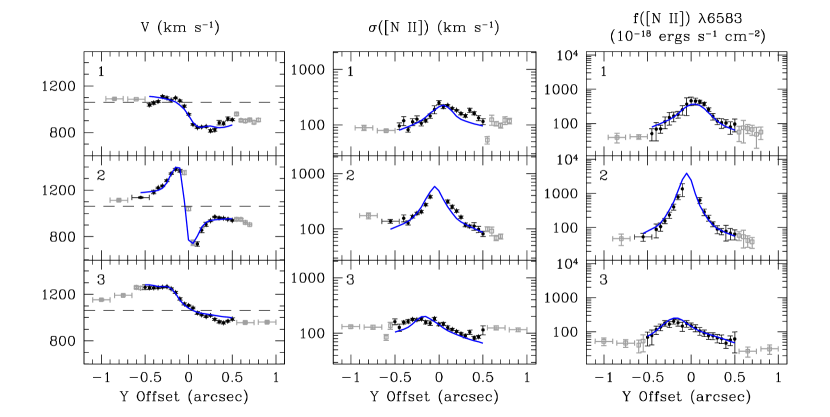
Figure 8.— Results of the final model with an asymmetric drift correction; see Figure 7 for description.

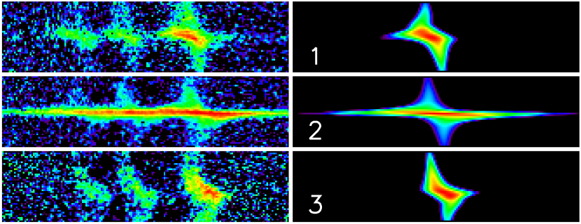
Figure 9.— Continuum-subtracted observed 2D STIS spectrum for the H$\alpha$ + [N II] region (left) and the synthetic 2D spectrum of the [N II] $\lambda 6583$ Å emission line from the final disk model with an asymmetric drift correction (right) for each of the three slit positions. The spatial axis is vertical and the wavelength axis is horizontal, with increasing wavelengths to the right. Each box is 93 Å in the dispersion direction and 2$\farcs$2 in the spatial direction. The numbers correspond to the slit locations depicted in Figure 1.

We explored the possibility that the intrinsic velocity dispersion contributes dynamical support to the gas disk by including an asymmetric drift correction in the model. Similar to the final model without an asymmetric drift correction, we calculated the disk model using a 0$\farcs$3-diameter PSF, $s=10$, and $r_{\mathrm{fit}}=$ 0$\farcs$5. We fixed $\Upsilon$ to 4 ($V$-band solar units), and excluded the three uncertain central velocity measurements from the fit. We also included an intrinsic radial velocity dispersion profile $\sigma_{r}$ as described in §5.4.

The asymmetric drift correction depends on the radial gradient in the number density of clouds in the disk, $\nu(r)$. We took $\nu$ to be given by the intrinsic emission-line flux distribution, as has done in the past (e.g., Barth et al., 2001; Coccato et al., 2006; Neumayer et al., 2007). In order to compute an azimuthally-averaged value for the radial derivative of $\nu$ in the asymmetric drift correction, we fit a revised model to the emission-line surface brightness profile, modeling it as an intrinsically circularly symmetric, inclined disk. The model for $\nu(r)$ contained three Gaussians and one exponential component (similar to that described in Table 1) but with the modification that all four components were forced to have the same centroid, ellipticity, and position angle. Using this model for $\nu(r)$, the asymmetric drift correction $v_{c}^{2}-v_{\phi}^{2}$ was then computed as a function of radius in each model calculation. The disk velocity field is then given by $v_{\phi}$.

When an asymmetric drift correction was included in the disk model calculations, the black hole mass increased to $8.5\times 10^{8}\ M_{\odot}$. This model is a better fit to the observed velocities, with $\chi^{2}=524.8$ and $\chi^{2}_{\nu}=10.1$, where 58 velocity measurements were fit with 6 free parameters. In Figure 8, we present the velocity, velocity dispersion, and flux from the final model with an asymmetric drift correction along with the observed velocity field. We also show the observed 2D STIS spectrum and the synthetic spectrum from the final model with an asymmetric drift correction for all three slit positions in Figure 9. This figure demonstrates that the rotating disk model is able to qualitatively match the complicated nature of the observed spectra. In the right column of Table 2 we provide the best-fit values of the model parameters.

6.3. Error Budget

We incorporated a number of sources of uncertainty in order to determine the final range of possible black hole masses. In addition to the formal model fitting uncertainties, we included the uncertainties associated with the stellar mass-to-light ratio and density profile, the PSF size, the subsampling factor, the fitting region, the analytical form of the emission-line flux profile, and the velocity measurements from the three central STIS rows. We additionally explored the variation in the black hole mass when several velocity measurements that appear to deviate from circular rotation are excluded from the fit. For the disk model with an asymmetric drift correction, we also included the contribution to the uncertainty resulting from the parametrization of the $\nu$. These sources of uncertainty are summarized below.

Model Fitting Uncertainty: We began by estimating the model fitting uncertainty. We explored the black hole mass parameter space between $3.2\times 10^{8}\ M_{\odot}$ and $6.2\times 10^{8}\ M_{\odot}$ for the disk model without an asymmetric drift correction, and from $(7.0-9.8)\times 10^{8}\ M_{\odot}$ for the model with the correction. We held $M_{\mathrm{BH}}$ fixed while the remaining parameters ($i$, $v_{\mathrm{sys}}$, $\theta$, $x_{\mathrm{offset}}$, and $y_{\mathrm{offset}}$) were allowed to vary. Before calculating these disk models, we rescaled the observed velocity uncertainties, which has been the common practice in previous work (e.g., Sarzi et al. 2001; Barth et al. 2001; de Francesco et al. 2006, 2008). We added 29 km s^-1 in quadrature to each of the observed velocity uncertainties in order to obtain $\chi^{2}_{\nu}\approx 1$ for the final model without an asymmetric drift correction. Likewise, we acquired $\chi^{2}_{\nu}\approx 1$ for the final model with an asymmetric drift correction by adding 28 km s^-1 in quadrature to the observed velocity uncertainties. By rescaling in this manner, the final uncertainty on the black hole mass will increase. This approach provides a conservative way in which to account for the detailed, small-scale velocity structure that our disk models fail to reproduce.

Figure 10 displays the results of the disk models. The range of black hole masses which caused $\chi^{2}$ to increase by 1.0 from the minimum value provides the 68.3% confidence limits (1$\sigma$ uncertainties) on $M_{\mathrm{BH}}$. For the disk models without an asymmetric drift correction, the 1$\sigma$ uncertainty corresponds to $(4.0-4.8)\times 10^{8}\ M_{\odot}$, while the range of black hole masses is $(8.0-8.8)\times 10^{8}\ M_{\odot}$ for the disk models with the correction. The 99.7% confidence limits (3$\sigma$ uncertainties) on $M_{\mathrm{BH}}$ were found by searching for the range of black hole masses that caused the minimum $\chi^{2}$ to increase by 9.0. The 3$\sigma$ uncertainties corresponded to $(3.5-5.7)\times 10^{8}\ M_{\odot}$ for the disk models without an asymmetric drift correction and to $(7.4-9.6)\times 10^{8}\ M_{\odot}$ for the models with the correction. These estimates also account for the small uncertainties associated with the parameters $i$, $v_{\mathrm{sys}}$, $\theta$, $x_{\mathrm{offset}}$, and $y_{\mathrm{offset}}$.

Figure 10.— Results of models without an asymmetric drift correction (left) and including the correction (right) using a 0$\farcs$3-diameter PSF, $s=10$, and $r_{\mathrm{fit}}=$ 0$\farcs$5. For each model, $M_{\mathrm{BH}}$ was held fixed while $i$, $\theta$, $v_{\mathrm{sys}}$, $x_{\mathrm{offset}}$, and $y_{\mathrm{offset}}$ were allowed to vary such that $\chi^{2}$ was minimized. The dashed and dotted horizontal lines denote where $\chi^{2}$ has increased by 1.0, and 9.0, from the minimum value, corresponding to 1$\sigma$, and 3$\sigma$, uncertainties on $M_{\mathrm{BH}}$, respectively.

We found that rescaling the uncertainties on the observed velocities resulted in a slightly different best-fit black hole mass than the mass found from our final model with an asymmetric drift correction presented in §6.2. However, the black hole mass found from our final model with an asymmetric drift correction still falls within the 1$\sigma$ model fitting uncertainty. Similar behavior has been seen in the previous analysis of NGC 1300 and NGC 2748 by Atkinson et al. (2005). We choose to apply the fractional model fitting error found above to the best-fit $M_{\mathrm{BH}}$ from the final model presented in §6.2. Below, we describe the additional contributions to the error budget.

Stellar Mass-to-Light Ratio and Density Profile: Fixing $\Upsilon=4$ does not have a large effect on the black hole mass, further emphasizing that the STIS data is fairly insensitive to the stellar contribution. We find that by allowing $\Upsilon$ to vary during the fit, the best-fit stellar mass-to-light ratio is $\Upsilon=0$ and the black hole mass is $M_{\mathrm{BH}}=4.8\times 10^{8}\ M_{\odot}$ for the model without an asymmetric drift correction. Thus, increasing the mass-to-light ratio from the best-fit value of $\Upsilon=0$ to $\Upsilon=4$ results in a 12% decrease in $M_{\mathrm{BH}}$. For the model with an asymmetric drift correction, allowing $\Upsilon$ to vary during the fit caused $M_{\mathrm{BH}}$ to change by only 1% from the best-fit mass, while $\Upsilon$ decreased to 2.6 $V$-band solar units.

Also, as discussed in §5.1 and shown in Figure 4, the uncertainty related to the exclusion of the central compact component from the mass budget is unlikely to affect our $M_{\rm BH}$ measurement. In fact, even if all the nuclear light is assigned a mass meaning, the black hole mass remains the same at $8.5\times 10^{8}\ M_{\odot}$ and drops to $4.1\times 10^{8}\ M_{\odot}$ (a 5% change from the best-fit mass), with and without asymmetric drift correction, respectively.

PSF size: When PSFs of different sizes (0$\farcs$3 – 0$\farcs$6 in diameter) were used in the calculation of the model without an asymmetric drift correction, the black hole mass varied between $(4.3-4.5)\times 10^{8}\ M_{\odot}$ with a root-mean-square (rms) scatter of $8.7\times 10^{6}\ M_{\odot}$. This corresponds to 2% of the best-fit black hole mass. Similarly, for the model with an asymmetric drift correction, the black hole mass varied between $8.5\times 10^{8}\ M_{\odot}$ and $8.6\times 10^{8}\ M_{\odot}$ with an rms scatter equal to $4.3\times 10^{6}\ M_{\odot}$, or 1% of the best-fit black hole mass.

Subsampling Factor: For disk models without an asymmetric drift correction, using subsampling factors ranging from $s=2$ to $s=10$ resulted in black hole masses between $M_{\mathrm{BH}}=4.1\times 10^{8}\ M_{\odot}$ and $4.3\times 10^{8}\ M_{\odot}$ with a rms scatter of only $7.5\times 10^{6}\ M_{\odot}$, or 2% of the best-fit black hole mass. The black hole mass ranged from $(8.2-8.6)\times 10^{8}\ M_{\odot}$ for disk models with an asymmetric drift correction. The rms scatter was $1.4\times 10^{7}\ M_{\odot}$, which is 2% of the best-fit black hole mass.

Fitting Region: For the disk models without an asymmetric drift correction, the black hole mass varied between $M_{\mathrm{BH}}=4.2\times 10^{8}\ M_{\odot}$ and $4.5\times 10^{8}\ M_{\odot}$ for fitting regions between 0$\farcs$3 and 1″. The rms scatter in $M_{\mathrm{BH}}$ was small at $1.3\times 10^{7}\ M_{\odot}$, or 3% of the best-fit black hole mass. The best-fit black hole mass for models with an asymmetric drift correction varied between $(8.2-8.7)\times 10^{8}\ M_{\odot}$, with an rms scatter that amounted to $1.6\times 10^{7}\ M_{\odot}$, corresponding to 2% of the best-fit mass.

Emission-Line Flux: The dynamically cold, thin-disk models with different parametrizations of the emission-line flux (previously described in §6) returned best-fit masses between $4.2\times 10^{8}\ M_{\odot}$ and $4.7\times 10^{8}\ M_{\odot}$. The rms scatter was $1.6\times 10^{7}\ M_{\odot}$, or 4% of the best-fit black hole mass. When the different emission-line flux models were used to weight the line-of-sight velocity profiles in the model with an asymmetric drift correction, we found that the black hole mass fluctuated between $8.1\times 10^{8}\ M_{\odot}$ and $8.9\times 10^{8}\ M_{\odot}$ with an rms scatter of $2.7\times 10^{7}\ M_{\odot}$, or 3% of the best-fit $M_{\mathrm{BH}}$.

Velocity Measurements Within 0$\farcs$05 of the Nucleus: We calculated a disk model without an asymmetric drift correction in which the three innermost velocity measurements were included in the fit, as a comparison to the final model that excludes these uncertain measurements. The black hole mass decreased by just 2% to $M_{\mathrm{BH}}=4.2\times 10^{8}\ M_{\odot}$. The inclusion of the velocity measurements from the three innermost STIS rows also had an insignificant impact on $M_{\mathrm{BH}}$ for the model with asymmetric drift correction; $M_{\mathrm{BH}}$ decreased by 1% from the best-fit mass. Because the sphere of influence is well resolved by the STIS data, excluding the three central velocity measurements during the fit has a small effect on the black hole mass.

Excluding Several Velocity Measurements that Deviate from Circular Rotation: The final models with and without an asymmetric drift correction match the overall shape of the observed velocity curves well, but are unable to reproduce all of the velocity features, resulting in moderate $\chi^{2}_{\nu}$ values of 10.1 and 11.4, respectively. In order to measure the impact of several velocity measurements that show localized departures from pure circular rotation on the black hole mass and $\chi^{2}_{\nu}$, we fit models with and without an asymmetric drift correction to various data sets. We constructed data sets in which we removed anywhere from a single velocity measurement to ten velocity data points that appeared to be discrepant from the final models presented in §6.1 and §6.2, such as the points at Y-Offset -0.45” to -0.35” from slit position 1, the point at Y-Offset -0.55” from slit position 2, and the points at Y-Offset 0.30” to 0.45” from slit position 3. For the model without an asymmetric drift correction, we found that the black hole mass varied between $4.1\times 10^{8}\ M_{\odot}$ and $4.3\times 10^{8}\ M_{\odot}$, with an rms deviation of just 2% of the best-fit mass, and the lowest $\chi^{2}_{\nu}$ was 6.1. Similarly, for the model with an asymmetric drift correction, the rms deviation in the black hole mass was 1% of the best-fit mass, varying between $(8.3-8.5)\times 10^{8}\ M_{\odot}$, with the lowest $\chi^{2}_{\nu}$ being 5.3. Thus, the quality of the fit to the observed velocity curves improves significantly, while the black hole mass remains roughly constant. This lends further support that the best-fit masses from our final models with and without an asymmetric drift correction are trustworthy despite the moderate $\chi^{2}_{\nu}$ values.

Number Density of Clouds: For models with an asymmetric drift correction, we also tested a variety analytical functions for $\nu$. These distributions included both shallow and steep profiles, and ranged in complexity with anywhere from two to six components. The functions were composed of intrinsic circularly-symmetric Gaussians and exponentials. When calculating the models, we continued to weight the line-of-sight velocity profiles by the 3 Gaussians $+$ 1 exponential emission-line flux model (model A) discussed in §5.2. The effect on the black hole mass was small, and we measured masses between $(7.1-8.6)\times 10^{8}\ M_{\odot}$ with an rms scatter of $5.6\times 10^{7}\ M_{\odot}$, which is 7% of the best-fit black hole mass.

All of the above sources of uncertainty were added in quadrature to the model-fitting uncertainty. The final range of black hole masses for the cold thin-disk model is $(3.6-5.1)\times 10^{8}\ M_{\odot}$ (1$\sigma$ uncertainties) and $(3.3-5.8)\times 10^{8}\ M_{\odot}$ (3$\sigma$ uncertainties) with a best-fit black hole mass of $4.3\times 10^{8}\ M_{\odot}$. For the disk model with an asymmetric drift correction, the final range of masses is $(7.7-9.4)\times 10^{8}\ M_{\odot}$ (1$\sigma$ uncertainties) and $(7.3-10.0)\times 10^{8}\ M_{\odot}$ (3$\sigma$ uncertainties) with a best-fit black hole mass of $8.5\times 10^{8}\ M_{\odot}$.

7. Discussion

By modeling the M84 emission-line gas kinematics as a dynamically cold, thin disk in circular rotation, we find a best-fit black hole mass of $(4.3^{+0.8}_{-0.7})\times 10^{8}\ M_{\odot}$. Incorporating an asymmetric drift correction in our disk model results in a best-fit black hole mass of $(8.5^{+0.9}_{-0.8})\times 10^{8}\ M_{\odot}$. We favor the disk model with an asymmetric drift correction because it is physically plausible that the intrinsic turbulence affects the disk’s dynamics and also because the model provides a better fit to the observed radial velocities.

There are a few caveats associated with the asymmetric drift correction worth mentioning. Our treatment of the asymmetric drift correction is only an approximation, and the black hole mass measurement becomes increasingly less certain as $\sigma_{r}/v_{c}$ approaches $\sim 1$. In the case of M84, we find that $\sigma_{r}/v_{c}$ can reach moderate values of 0.57 (see Figure 11). Moreover, the increase in the black hole mass when an asymmetric drift correction is applied is extremely large (a 98% change), and can be attributed to the very steep radial gradients in both $\nu$ and $\sigma_{r}$. While $\sigma_{r}$ is known fairly well through a fit to the observed line widths, the radial distribution of the number density of clouds in the disk is not known. Following past work, we have used the emission-line flux profile as a proxy for the density profile $\nu(r)$. While this is at best a rough approximation, we found that different parametrizations of $\nu$ did not result in substantial changes to the inferred black hole mass. However, if instead a very simplistic asymmetric drift correction is applied, where $v_{c}^{2}-v_{\mathrm{rot}}^{2}=\sigma_{r}^{2}$, the black hole mass decreases by $\sim 30$% to $M_{\mathrm{BH}}=6.0\times 10^{8}\ M_{\odot}$. Finally, the asymmetric drift correction is strictly applicable in the limit of collisionless particles, as in stellar dynamics. Here, we are applying the correction to gas clouds, which are not collisionless particles, and therefore the analogy is not perfect, although it is still a useful approximation (e.g., Valenzuela et al., 2007). Therefore, calculating a model which includes an asymmetric drift correction is an informative exercise, but only provides an approximate indication of the dynamical influence of the intrinsic velocity dispersion.

Additionally, dust obscuration is an issue in M84 and affects both our gas dynamical models. As can be seen in the WFPC2 $V$-band image in Figure 1, there are two prominent dust lanes within the central $\sim 4$″ that are oriented roughly east to west. Based on a $V-I$ color map, Bower et al. (1997) measure a dust mass of $7\times 10^{4}\ M_{\odot}$, and note that the dust extinction is the greatest along the northern portion of the central dust lane and at a patch located on the nucleus. The effects of dust on the determination of the stellar mass profile should be minimized, as the Kormendy et al. (2009) surface brightness profile uses NICMOS $H$-band data for the nuclear region. Also, as we have shown above, the model fits are insensitive to the stellar mass contribution because the black hole dominates over the region we are modeling. Dust extinction will affect the observed gas kinematics, however including these effects in the calculation requires radiative transfer models of the disk’s gas dynamics. Such modeling has yet to be applied to gas kinematical measurements and is beyond the extent of this paper.

Figure 11.— Ratio of $\sigma_{r}$ to $v_{c}$ as a function of distance from the M84 nucleus for the final model discussed in §6.2.

The best-fit black hole mass of $(8.5^{+0.9}_{-0.8})\times 10^{8}\ M_{\odot}$ is a factor of $\sim 2$ smaller than the mass measured by Bower et al. (1998) of $(1.5^{+1.1}_{-0.6})\times 10^{9}\ M_{\odot}$, although the two measurements are formally consistent within their quoted uncertainties. If we consider our best-fitting model that does not include asymmetric drift (perhaps a more fair comparison since Bower et al. did not include asymmetric drift), our result is a factor of $\sim 3$ smaller than theirs. While there are many factors that contribute to this difference, one reason is likely to be the different assumptions we have made about the structure of the velocity field. Bower et al. decomposed the emission lines into two distinct kinematic components, which they characterized as one rotating disk component and one unrelated, low-velocity component, while we have modeled the kinematics as arising from a single rotating disk. The observed and modeled line profiles of the central slit position, shown in Figure 9, help to illustrate the situation. Close to the nucleus, the emission lines flare out into a broad “fan” of emission with large line widths and complex, strongly non-Gaussian profiles, due to a combination of instrumental and rotational broadening, and the increase in the intrinsic velocity dispersion close to the nucleus. Maciejewski & Binney (2001) describe in detail how this fan of emission, which can mimic the appearance of two separate kinematic components, can be generated through the combination of rotational broadening and the effects of observing through a slit that is wider than the PSF core.

Moreover, our model calculation includes a more detailed treatment of the telescope and spectrograph optics than was carried out by Bower et al. (1998), and includes the full propagation of emission-line profiles through the spectrograph, rather than a simpler propagation of mean velocities. While it is difficult to pinpoint the exact cause of the difference in the resulting black hole mass, these are likely to be the primary reasons. Our results show that we can obtain a robust fit of a disk model to the data even in the absence of any measurements from the central three rows, where the line profiles are most severely blended and asymmetric and the velocity field is most strongly affected by PSF blurring.

Of the remaining disk model parameters, our best-fit systemic velocity and inclination angle of $v_{\mathrm{sys}}=1060$ km s^-1 and $i=72^{\circ}$ differ from the results of Bower et al. (1998), who found $v_{\mathrm{sys}}=1125$ km s^-1 and $i=80^{\circ}$. The systemic velocity determined through our modeling is in better agreement with the recession velocities given by the NASA Extragalactic Database (NED). The velocities quoted by NED were measured from optical lines, and ranged in value from 954 – 1119 km s^-1, with an average of 1025 km s^-1. Bower et al. (1998) did not fit for the relative angle between the STIS slit and the major axis of the gas disk. Rather, they took the disk position angle to be that of the major axis of the large-scale emission-line structure (83^∘ east of north) measured by Baum et al. (1998). In our disk models, we allowed $\theta$ to be a free parameter and found a similar position angle for the major axis of the gaseous disk. Our best-fit value is $\theta=28^{\circ}$, corresponding a disk major axis position angle of 76^∘ east of north. Also, Bower et al. (1998) adopted a stellar mass-to-light ratio of $\Upsilon=5$ ($V$-band solar units), comparable to the one fixed in our model of $\Upsilon=4$ ($V$-band solar units).

The comparison of our results with those of Maciejewski & Binney (2001) is less direct, since they did not carry out model fitting to the observed velocity field. Instead, they estimated the black hole mass based on the visual location of a caustic feature in the spectrum of the central slit position. This caustic results from the interplay between the disk rotation and the gradient in instrumental wavelength shifts across the slit. These two line-broadening effects can be oppositely directed and can effectively cancel each other out, resulting in a sharp reduction in the observed line width at a specific location in the disk. We do not clearly see evidence for this caustic feature in the 2D spectrum or in the measured emission-line widths, so we cannot reproduce their estimate of $M_{\mathrm{BH}}$. While such caustics should in principle occur in STIS spectra of emission-line disks, it is possible that the intrinsic line width in the M84 disk is so large that it washes out any observable signature of the caustic. We note, however, that our best-fitting model without asymmetric drift gives a result that is consistent with that of Maciejewski & Binney (2001).

With respect to the $M_{\mathrm{BH}}-\sigma_{\star}$ and $M_{\mathrm{BH}}-L$ relationships, our best-fit black hole mass for M84 of $(8.5^{+0.9}_{-0.8})\times 10^{8}\ M_{\odot}$ is a factor of $\sim 2$ smaller than the mass from Bower et al. (1998) that has been most often adopted in the relationships. This new mass measurement lies closer to the mass expected from the $M_{\mathrm{BH}}-\sigma_{\star}$ and $M_{\mathrm{BH}}-L$ relationships measured by Gültekin et al. (2009). Recent stellar dynamical studies of other galaxies, as well as our analysis of M84, show that some previous black hole mass measurements should be re-evaluated, and determination of the true shape and scatter of the $M_{\mathrm{BH}}-\sigma_{\star}$ and $M_{\mathrm{BH}}-L$ relationships is an evolving process that will continue to change as observations and modeling techniques continue to improve. Recent calibrations of the relations still include some of the early gas-dynamical measurements that were done with the FOS on HST, and these should be particularly important targets to revisit with future observations. Equally important are cross-checks between gas-dynamical and stellar-dynamical techniques within the same object, as each mass measurement method suffers from independent systematic uncertainties. In particular, gas-dynamical models would benefit tremendously from a better understanding of the physical origin and the dynamical influence of the intrinsic velocity dispersion.

8. Conclusions

With the goal of resolving the uncertainty in the M84 black hole mass, we have re-analyzed multi-slit archival HST STIS observations of the nuclear region of M84. We mapped out the 2-dimensional [N II] $\lambda 6583$ emission-line velocity, velocity dispersion, and flux. We then modeled the velocity field as a cold, thin disk in circular rotation. The line widths predicted by this model are smaller than the observed line widths, and we found that an intrinsic velocity dispersion is needed in order to match the observations. The additional velocity dispersion may have a dynamical origin and provide pressure support to the gaseous disk, thus we calculated a second disk model with an asymmetric drift correction. We found that the disk model with an asymmetric drift correction is a better fit to the data than the cold thin-disk model. This model gives a black hole mass of $(8.5^{+0.9}_{-0.8})\times 10^{8}\ M_{\odot}$ (1$\sigma$ uncertainties).

We have employed a more rigorous and comprehensive gas-dynamical model to measure the black hole mass in M84 than the previous two studies. In addition to calculating an asymmetric drift correction, we included a more sophisticated treatment of the effects of the telescope optics and interpreted the complex nuclear spectra as arising from a single gas component. We also performed an error analysis that encompasses a number of sources of uncertainty in order to determine the range of possible black hole masses.

Our new mass measurement for M84 is a factor of $\sim 2$ smaller than the Bower et al. (1998) value of $M_{\mathrm{BH}}=(1.5^{+1.1}_{-0.6})\times 10^{9}\ M_{\odot}$ and a factor of $\sim 2$ larger than the Maciejewski & Binney (2001) estimate of $M_{\mathrm{BH}}=4\times 10^{8}\ M_{\odot}$. The black hole mass given by Bower et al. (1998) is often used in the $M_{\mathrm{BH}}-\sigma_{\star}$ and $M_{\mathrm{BH}}-L$ relationships. Therefore, while recent stellar-dynamical work has found that several masses at the high-end of the black hole mass-host galaxy relationships have been underestimated by a factor of $\sim 2$, we find that the gas-dynamical black hole mass measurement for M84 has been overestimated by a factor of $\sim 2$. With this adjustment to the black hole mass, M84 lies closer to the mass expected from both the $M_{\mathrm{BH}}-\sigma_{\star}$ and $M_{\mathrm{BH}}-L$ relationships. Future work should thus aim to understand the systematics associated with each of the main mass measurement methods, and to re-examine those objects for which uncertain mass measurements remain.

References

- Atkinson et al. (2005) Atkinson, J. W., et al. 2005, MNRAS, 359, 504
- Barth et al. (2001) Barth, A. J., Sarzi, M., Rix, H.-W., Ho, L. C., Filippenko, A. V., & Sargent, W. L. W. 2001a, ApJ, 555, 685
- Barth et al. (2001b) Barth, A. J., Sarzi, M., Ho, L. C., Rix, H.-W., Shields, J. C., Filippenko, A. V., Rudnick, G., Sargent, W. L. W. 2001b, in The Central Kiloparsec of Starbursts and AGNs, ed. J. H. Knapen, J. K. Beckman, I. Shlosman, & T. J. Mahoney (San Francisco: ASP), 370
- Baum et al. (1998) Baum, S. A., Heckman, T. M., Bridle, A., van Breugel, W. J. M., & Miley, G. K. 1998, ApJS, 68, 643
- Bell et al. (2003) Bell, E. F., McIntosh, D. H., Katz, N., & Weinberg, M. D. 2003, ApJS, 149, 289
- Bower et al. (1997) Bower, G. A., Heckman, T. M., Wilson, A. S., & Richstone, D. O. 1997, ApJ, 483, L33
- Bower et al. (1998) Bower, G. A., et al. 1998, ApJ, 492, L111
- Bower et al. (2000) Bower, G. A., et al. 2000, ApJ, 534, 189
- Capetti et al. (2005) Capetti, A., Marconi, A., Macchetto, D., & Axon, D. 2005, A&A, 431, 465
- Coccato et al. (2006) Coccato, L., Sarzi, M., Pizzella, A., Corsini, E. M., Dalla Bonta, E., & Bertola, F. 2006, MNRAS, 366, 1050
- Dalla Bontà et al. (2009) Dalla Bonta, E., Ferrarese, L., Corsini, E. M., Miralda-Escude, J., Coccato, L., Sarzi, M., Pizzella, A., & Beifiori, A. 2009, ApJ, 690, 537
- de Francesco et al. (2006) de Francesco, G., Capetti, A., & Marconi, A. 2006, A&A, 460, 439
- de Francesco et al. (2008) de Francesco, G., Capetti, A., & Marconi, A. 2008, A&A, 479, 355
- de Vaucouleurs et al. (1991) de Vaucouleurs, G., de Vaucouleurs, A., Corwin, H. G., Buta, R. J., Paturel, G., & Fouque, P. 1991, Third Reference Catalogue of Bright Galaxies (New York: Springer-Verlag)
- Ferrarese et al. (1996) Ferrarese, L., Ford, H. C., & Jaffe, W. 1996, ApJ, 470, 444
- Ferrarese & Ford (1999) Ferrarese, L., & Ford, H. C. 1999, ApJ, 515, 583
- Ferrarese & Merritt (2000) Ferrarese, L., & Merritt, D. 2000, ApJL, 539, L9
- Gebhardt et al. (2000) Gebhardt, K., et al. 2000, ApJL, 539, L13
- Gebhardt & Thomas (2009) Gebhardt, K., & Thomas, J. 2009, ApJ, 700, 1690
- Gültekin et al. (2009) Gültekin, K., et al. 2009, ApJ, 698, 198
- Harms et al. (1994) Harms, R. J., et al. 1994, ApJ, 436, L35
- Hicks & Malkan (2008) Hicks, E. K. S., & Malkan, M. A. 2008, ApJS, 174, 31
- Ho et al. (1997) Ho, L. C., Filippenko, A. V., & Sargent, W. L. W. 1997a, ApJS, 112, 315
- Kormendy et al. (2009) Kormendy, J., Fisher, D. B., Cornell, M. E., & Bender, R. 2009, ApJS, 182, 216
- Kormendy & Bender (1996) Kormendy, J., & Bender, R. 1996, ApJ, 464, L119
- Kormendy & Gebhardt (2001) Kormendy, J. & Gebhardt, K. 2001, in The 20th Texas Symposium on Relativistic Astrophysics, ed. H. Martel and J. C. Wheeler (Melville: AIP), 363
- Krist & Hook (2004) Krist, J., & Hook, R. 2004, The Tiny Tim User’s Guide (Baltimore:STScI)
- Lauer et al. (2007) Lauer, T. R., et al. 2007, ApJ, 662, 808
- Macchetto et al. (1997) Macchetto, F. Marconi, A., Axon, D. J., Capetti, A., Sparks, W., & Crane, P. 1997, ApJ, 489, 579
- Maciejewski & Binney (2001) Maciejewski, W., & Binney, J. 2001, MNRAS, 323, 831
- Marconi et al. (2003) Marconi, A., et al. 2003, ApJ, 586, 868
- Marconi et al. (2006) Marconi, A., Pastorini, G., Pacini, F., Axon, D. J., Capetti, A., Macchetto, D., Koekemoer, A., & Schreier, E. J. 2006, A&A, 448, 921
- Markwardt (2009) Markwardt, C. B. 2009, in ASP Conf. Ser. 411, Astronomical Data Analysis Software and Systems XVIII, ed. D. A. Bohlender, D. Durand, & P. Dowler (San Francisco: ASP), 251
- Monnet, Bacon, & Emsellem (1992) Monnet, G., Bacon, R. & Emsellem, E. 1992, A&A, 253, 366
- Neumayer et al. (2007) Neumayer, N., Cappellari, M., Reunanen, J., Rix, H.-W., van der Werf, P. P., de Zeeuw, P. T., & Davies, R. I. 2007, ApJ, 671, 1329
- Pastorini et al. (2007) Pastorini, G., et al. 2007, A&A, 469, 405
- Peng et al. (2002) Peng, C. Y., Ho, L. C., Impey, C. D., & Rix, H.-W. 2002, AJ, 124, 266
- Press et al. (1992) Press, W. H., Teukolsky, S. A., Vetterling, W. T., & Flannery, B. P. 1992, Numerical Recipes (Cambridge: Cambridge Univ. Press)
- Sarzi et al. (2001) Sarzi, M., Rix, H.-W., Shields, J. C., Rudnick, G., Ho, L. C., McIntosh, D. H., Filippenko, A. V., & Sargent, W. L. W. 2001, ApJ, 550, 65
- Sarzi et al. (2002) Sarzi, M., et al. 2002, ApJ, 567, 237
- Shapiro et al. (2006) Shapiro, K. L., Cappellari, M., de Zeeuw, T., McDermid, R. M., Gebhardt, K., van den Bosch, R. C. E., & Statler, T. S. 2006, MNRAS, 370, 559
- Shen & Gebhardt (2010) Shen, J., & Gebhardt, K. 2010, ApJ, 711, 484
- Tremaine et al. (2002) Tremaine, S., et al. 2002, ApJ, 574, 740
- Valenzuela et al. (2007) Valenzuela, O., Rhee, G., Klypin, A., Governato, F., Stinson, G., Quinn, T., & Wadsley, J. 2007, ApJ, 657, 773
- van den Bosch & de Zeeuw (2010) van den Bosch, R. C. E., & de Zeeuw, P. T. 2010, MNRAS, 401, 1770
- van der Marel & van den Bosch (1998) van der Marel, R. P., & van den Bosch, F. C. 1998, AJ, 116, 2220
- van Dokkum (2001) van Dokkum, P. G. 2001, PASP, 113, 1420
- Verdoes Kleijn et al. (2000) Verdoes Kleijn, G. A., van der Marel, R. P., Carollo, C. M., & de Zeeuw, P. T. 2000, AJ, 120, 1221
- Verdoes Kleijn et al. (2002) Verdoes Kleijn, G. A., van der Marel, R. P., de Zeeuw, P. T., Noel-Storr, J., Baum, S. A. 2002, AJ, 124, 2524
- Verdoes Kleijn, van der Marel, & Noel-Storr (2006) Verdoes Kleijn, G. A., van der Marel, R. P., & Noel-Storr, J. 2006, AJ, 131, 1961
- Walsh et al. (2008) Walsh, J. L., Barth, A. J., Ho, L. C., Filippenko, A. V., Rix, H.-W., Shields, J. C., Sarzi, M., & Sargent, W. L.W. 2008, AJ, 136, 1677
- Wold et al. (2006) Wold, M., Lacy, M., Kaufl, H. U., & Siebenmorgen, R. 2006, A&A, 460, 449