A translucent interstellar cloud at $z=2.69$:

We present the analysis of a sub-Damped Lyman-$\alpha$ system with neutral hydrogen column density, $\log N$(H⁰) (${\rm cm}^{-2}$) = 20.0$\pm$0.15 at $z_{\rm abs}$ = 2.69 toward SDSS J123714.60$+$064759.5 ($z_{\rm em}$ = 2.78). Using the VLT/UVES and X-shooter spectrographs, we detect H₂, HD and CO molecules in absorption with $\log N$(H₂, HD, CO) (${\rm cm}^{-2}$) = 19.21${}^{+0.13}_{-0.12}$, 14.48$\pm$0.05 and 14.17$\pm$0.09 respectively. The overall metallicity of the system is super-solar ([Zn/H] = +0.34 relative to solar) and iron is highly depleted ([Fe/Zn] = $-1.39$), revealing metal-rich and dusty gas. Three H₂ velocity cxomponents spanning $\sim$125 km s^-1 are detected. The strongest H₂ component, at $z_{\rm abs}$ = 2.68955, with $\log N$(H₂) = 19.20, does not coincide with the centre of the H i absorption. This implies that the molecular fraction in this component, $f_{\rm H2}$ = 2$N$(H₂)/(2$N$(H₂)+$N$(H⁰)), is larger than the mean molecular fraction $\left<f_{\rm H2}\right>$ = 1/4 in the system. This is supported by the detection of Cl⁰ associated with this H₂ component having $N$(Cl⁰)/$N$(Cl⁺) $>$ 0.4. Since Cl⁰ is tied up to H₂ by charge exchange reactions, this means that the molecular fraction in this component is not far from unity. The kinetic temperature derived from the J = 0 and 1 rotational levels of H₂ is $T$ = 108${}^{+84}_{-33}$ K and the particle density derived from the C⁰ ground-state fine structure level populations is $n_{\rm H0}$ $\sim$ 50-60 cm^-3. We derive an electronic density $<$2 cm^-3 for a UV field similar to the Galactic one and show that the carbon to sulphur ratio in the cloud is close to the solar ratio. The size of the molecular cloud is probably smaller than 1 pc. Both the CO/H₂ = 10^-5 and CO/C⁰ $\sim$ 1 ratios for $f_{\rm H2}$ $>$ 0.24 indicate that the cloud classifies as translucent, i.e., a regime where carbon is found both in atomic and molecular form. The corresponding extinction, $A_{\rm V}=0.14$, albeit lower than the definition of a translucent sightline (based on extinction properties), is high for the observed H⁰ column density. This means that intervening clouds with similar local properties but with larger column densities (i.e. larger physical extent) could be missed by current magnitude-limited QSO surveys. The excitation of CO is dominated by radiative interaction with the Cosmic Microwave Background Radiation (CMBR) and we derive $T_{\rm ex}$(CO) = 10.5${}^{+0.8}_{-0.6}$ K when $T_{\rm CMBR}$($z$=2.69) = 10.05 K is expected. We measure $N(\mbox{HD})/2N(\mbox{H${}_{2}$})=10^{-5}$. This is about 10 times higher than what is measured in the Galactic ISM for $f_{\rm H2}=1/4$ but similar to what is measured in the Galactic ISM for larger molecular fractions. The astration factor of deuterium – with respect to the primordial D/H ratio – is only about 3. This can be the consequence of accretion of unprocessed gas from the intergalactic medium onto the associated galaxy. In the future, it will be possible to search efficiently for molecular-rich DLAs/sub-DLAs with X-shooter but detailed studies of the physical state of the gas will still need UVES observations.

1 Introduction

Studies of the Interstellar Medium (ISM) in the local Universe have shown that the neutral ISM presents a complex structure, with cold and dense clouds immersed in a warmer and more diffuse medium. These different ISM phases should be detectable at high redshift by their absorption signatures in Damped Lyman-$\alpha$ (DLA) systems observed in quasar spectra (Petitjean et al., 1992). However, although there are evidences of the multiphase nature of DLA systems (e.g. Wolfe et al., 2004), most of the intervening DLAs probe only warm ($T\ga 3000$ K) and diffuse ($n_{\rm H}<1$ ${\rm cm}^{-2}$) atomic gas (e.g. Petitjean et al., 2000; Kanekar & Chengalur, 2003). The reason is that the cross-sections of the different phases are quite different and it is not possible to sample them equally well.

Searching for molecular hydrogen in high redshift DLAs (Ledoux et al., 2003; Petitjean et al., 2006; Noterdaeme et al., 2008a) is an efficient way of detecting colder and denser neutral gas and to probe its physical conditions (e.g. Reimers et al., 2003; Cui et al., 2005; Hirashita & Ferrara, 2005; Srianand et al., 2005; Ledoux et al., 2006b; Noterdaeme et al., 2007a, b). These studies have shown that molecular hydrogen is confined in small clouds (pc-sized) with densities $n\sim$ 1-100 cm^-3 and temperatures $T\sim$ 70-200 K. The filling factor of H₂-bearing clouds in DLAs is much less than one and only 10 % of the lines of sight through a DLA galaxy do intercept H₂-bearing clouds down to a limit of $N$(H${}_{2})\sim 10^{14}\leavevmode\nobreak\ {\rm cm}^{-2}$ (Noterdaeme et al., 2008a). H₂-bearing clouds in DLAs have small physical extents. Direct evidence for this is given by the fact that the intervening H₂-bearing gas does not completely fill the beam from the broad line region of the quasar Q 1232+082 (Ivanchik et al. 2010; Balashev et al., submitted). Nonetheless, the molecular fraction in DLAs remains small and typical of what is seen in Galactic diffuse atomic gas with $f_{\rm H2}=2N(\mbox{H${}_{2}$})/(2N(\mbox{H${}_{2}$})+N($H${}^{0}))<0.1$ and often much lower than this (Ledoux et al., 2003; Noterdaeme et al., 2008a).

Snow & McCall (2006) have classified Galactic interstellar clouds into the following categories: (i) diffuse atomic, with low molecular fractions; (ii) diffuse molecular, where the fraction of hydrogen in molecules becomes substantial ($f_{\rm H2}>0.1$) but carbon is still mainly in ionised form (C⁺); (iii) translucent (first introduced by van Dishoeck & Black, 1989), where the carbon makes the transition to molecular; and (iv) dense molecular, where both hydrogen and carbon are fully molecular. As discussed above, most of the H₂-bearing DLAs detected so far are part of the first, and maybe for some of them, part of the second categories. The fourth category may be difficult to detect in absorption because of the high extinction such a cloud produces on the background source.

Despite their highly interesting chemistry and their close connection with star formation, we know very little about translucent clouds (i.e., the third category) at high redshift. The small cross-section of these clouds and/or the induced extinction of the light from the background sources can probably explain the absence of detection in more than three decades of QSO absorption-line research. However, observing molecular-rich gas in absorption should be possible by selecting sightlines passing through or starting from star-forming regions.

Since long-duration Gamma-Ray Bursts (GRBs) are known to occur within star-forming regions, absorption lines at the host-galaxy redshifts which are imprinted in GRB optical afterglow spectra (e.g., Fynbo et al., 2009) are obvious targets towards this goal. Nevertheless, current samples are characterised by a general lack of H₂ detection (e.g., Fynbo et al., 2006; Tumlinson et al., 2007). This is probably due to the still limited sample sizes as well as a bias against dusty – molecular-rich – lines of sight (Ledoux et al., 2009; Fynbo et al., 2009). The first detection of both H₂ and CO in the low-resolution spectrum of a highly reddened GRB afterglow (Prochaska et al., 2009) seems to confirm this scenario. Moreover, the observed molecular excitation is high in this case, indicating strong UV pumping from the GRB afterglow itself.

With the large number of quasar spectra available in the Sloan Digital Sky Survey (SDSS), it becomes possible to select the rare sightlines passing through intervening molecular-rich gas. However, due to the small cross-section of such clouds, an efficient selection must be applied. In the local ISM, carbon is found to transition from a ionised state (C⁺) to neutral (C⁰) and molecular form (CO) from the most superficial to the deepest parts of the clouds (e.g. Snow & McCall, 2006; Burgh et al., 2010). From our Very Large Telescope (VLT) survey for H₂ in DLAs (Ledoux et al., 2003; Noterdaeme et al., 2008a), it appears that C⁰ is generally observed in the same components as H₂. This is due to the photo-ionisation potential of C⁰ being similar to the energy of photons that dissociate H₂. However, the neutral fraction of carbon is generally small, probably because the gas is not completely shielded. This explains the non-detection of CO in these H₂-bearing DLAs, even down to $N($CO$)\sim 10^{12}$ ${\rm cm}^{-2}$  (e.g. Petitjean et al., 2002). Searching for systems with large column densities of neutral carbon could be an efficient way to select more shielded gas where other molecules can survive, without relying on a pre-selection based on the H⁰ column density (i.e. the absorbers need not be DLAs). Since several C i lines are located redwards of the Lyman-$\alpha$ forest, it is possible to search for strong C i absorptions directly in SDSS spectra using automatic procedures. We therefore initiated a program to survey with the VLT such specific sightlines. Our selection has been very successful and already allowed us to detect carbon monoxide along QSO sightlines for the first (Srianand et al., 2008b) and second times (Noterdaeme et al., 2009a). We present here the third detection of CO, at $z=2.69$ towards SDSS J123714.60$+$064759.5 ($z_{\rm em}=2.78$, hereafter called J 1237$+$0647). This is a beautiful and peculiar case for which detailed analysis of the physical properties of the gas is possible. We present the observations in Sect. 2, the measurement and results in Sect. 3 and provide some discussion in Sect. 4. We summarise our findings in Sect. 5.

2 Observations

Table 1: Journal of observations

Instrument	Date	Setting	Exposure time		Resolving power	SNR
UVES	27-03-2009	390+564	2$\times$5400 s	$\bigg{\}}$	390B:51400 - 564L:50800 - 564U:49500 - 775L:50200 -775U:48600	10-40
UVES	29-03-2009	390+564	2$\times$5400 s
UVES	27-04-2009	390+775	2$\times$4500 s
X-shooter	24-02-2010	UVB	3600 s	$\Big{\}}$	5100	50
X-shooter	03-03-2010	UVB	3600 s

2.1 X-shooter observations

We are conducting an observing campaign with X-shooter mounted on the Cassegrain focus of the VLT Unit 2-Kueyen telescope to study the molecular content of our complete sample of C⁰ absorbers. As a test case for the sensitivity of X-shooter in the blue, we observed J 1237$+$0647 ($g=19.2$) twice in service mode on February 24 (airmass 1.2; seeing 1.4$\arcsec$) and March 3, 2010 (airmass 1.3; seeing 1.2$\arcsec$), using a slit width of 1$\arcsec$ in the UVB arm. Each observation run consisted in 1 h exposure taken in staring mode (see Table 1). This yields the nominal resolution power of R = 5100 in the UVB arm and a signal-to-noise ratio of about 50 at $\sim$500 nm. Data were reduced using version 0.9.5 of the preliminary ESO X-shooter pipeline (Goldoni et al., 2006) and the appropriate calibration data. The two individual spectra were then combined weighting each pixel by the inverse of the error variance. A portion of the X-shooter spectrum featuring CO is shown on Fig. 1, where several electronic bands of CO are clearly detected. These bands are resolved into individual rotational levels in the UVES spectrum obtained with 8.5 h of exposure time (inset figures). From this, it is apparent that X-shooter is the most efficient instrument to survey a complete sample of candidates down to quasar magnitudes as faint as $r\sim 21.5$, whereas using UVES would be excessively time consuming. Then, but only in the case of detection, higher spectral resolution is needed to make a detailed analysis of the physical state of the gas as done in the following.

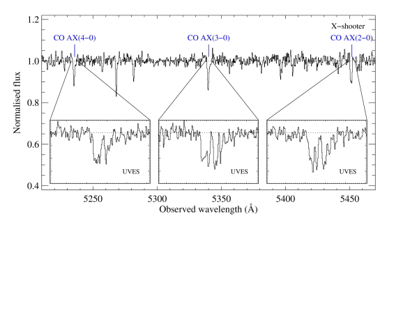
Figure 1: Portion of X-shooter spectrum in the UVB. The inset figures show 5 Å-wide portions of the UVES spectrum around the position of the detected electronic bands of CO.

2.2 UVES observations

The quasar J 1237$+$0647 was observed in visitor mode on March 27 and 29, 2009 and April 27, 2009 with the Ultraviolet and Visual Echelle Spectrograph (UVES; Dekker et al., 2000), mounted at the Nasmyth B focus of VLT-UT2. The total exposure time on source is 8.5 h (see Table 1). We used two dichroic settings (4$\times$5400 s with 390+564 and 2$\times$4500 s with 390+775) to cover the wavelength range 3300-9600 Å with small gaps at 4517-4621, 5597-5677 and 7764-7809 Å. The CCD pixels were binned $2\times 2$ and the slit width adjusted to 1$\arcsec$, yielding a resolving power of $\sim$50 000 under seeing conditions of 0.9-1$\arcsec$. Individual science spectra were reduced using the ESO UVES pipeline, which performs accurate sky subtraction while removing cosmic ray impacts at the same time. The spectra were then combined using a dedicated IDL routine by weighting each pixel by the inverse of the error variance in that pixel and clipping residual cosmic rays impacts that remained after the cleaning of 2D spectra.

3 Analysis

The system at $z=2.69$ towards J 1237$+$0647 features numerous absorption lines from atomic (H⁰, O⁰, C⁰, Mg⁰, Cl⁰ and S⁰), singly-ionised (Fe⁺, Si⁺, Zn⁺, Ni⁺, S⁺, C⁺), and molecular species (two isotopomers of molecular hydrogen: H₂ and HD; as well as carbon monoxide: CO).

We analysed the UVES spectrum using standard Voigt profile fitting techniques. The fits were performed through $\chi^{2}$-minimisation using the code FITLYMAN (Fontana & Ballester, 1995) which is available as a context of the ESO-MIDAS data analysis software. The spectrum was normalised in the wavelength ranges of interest by fitting spline functions to regions free from absorption lines. Atomic data were taken from Morton (2003) for metal lines, unless otherwise specified. Wavelengths and oscillator strengths were taken from Morton & Noreau (1994) and Eidelsberg & Rostas (2003) for CO and from Abgrall & Roueff (2006) for HD. Updated wavelengths of H₂ Lyman and Werner bands were taken from Bailly et al. (2010), with oscillator strengths from the Meudon group, based on calculations described in Abgrall et al. (1994). Photospheric solar abundances are taken from Asplund et al. (2009).

3.1 Atomic hydrogen

From the damped Lyman-$\alpha$ absorption line (see Fig. 2), we measure the total column density of atomic hydrogen to be $\log N($H${}^{0})({\rm cm}^{-2})=20.00\pm 0.15$, which is in agreement with the value measured automatically by Noterdaeme et al. (2009b) from the low resolution SDSS spectrum ($20.15\pm 0.28$). The centroid of the H i profile is well constrained by the Lyman-$\beta$ and Lyman-$\gamma$ absorption lines. The large Doppler parameter ($b\sim 100$ ${\rm km\,s^{-1}}$) required to fit the Lyman-$\beta$ and Lyman-$\gamma$ lines is a consequence of the presence of multiple components as testified by the clumpy profile of the O i$\lambda$1302 absorption line spread over $\sim$350 km s^-1 (see Fig. 2). We recall that O⁰ closely follows H⁰ because of favourable charge-exchange reaction. Unfortunately, because of strong saturation and blending effects, it is not possible to derive column densities in individual components and only the total H⁰ column density along the line of sight is accessible.

In Fig. 2 and subsequent figures and tables, the zero of the velocity scale is taken at the position of the CO component ($z_{\rm abs}$ = 2.68957, see Sect. 3.5) and the centroid of the three detected H₂ components at $z_{\rm abs}$ = 2.68801, 2.68868 and 2.68955 ($\Delta v$ = $-$127, $-$73, $-$1.6 km s^-1, see Sect. 3.3) are indicated by short vertical marks. Interestingly, the centroid of the atomic hydrogen absorption profile (vertical dotted line in Fig. 2 at $z_{\rm abs}$ = 2.69063) is shifted by about $+$86$\pm$10 km s^-1 relative to the CO absorption feature. This, the clumpy O i profile, and the large value of the $b$-parameter of H i lines, all indicate that a significant fraction of the atomic gas is not associated with the molecular gas. We will discuss this further down in more details.

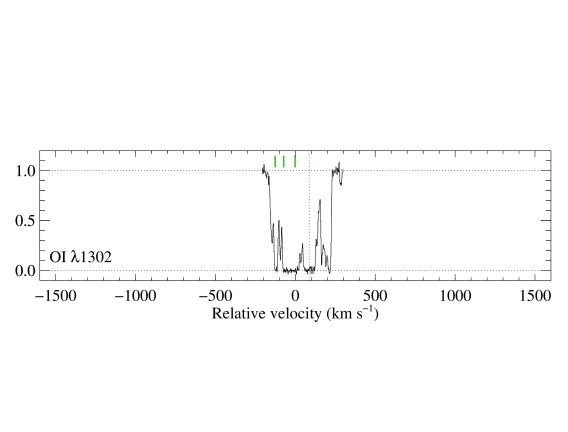
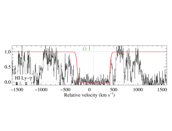
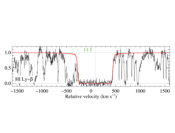
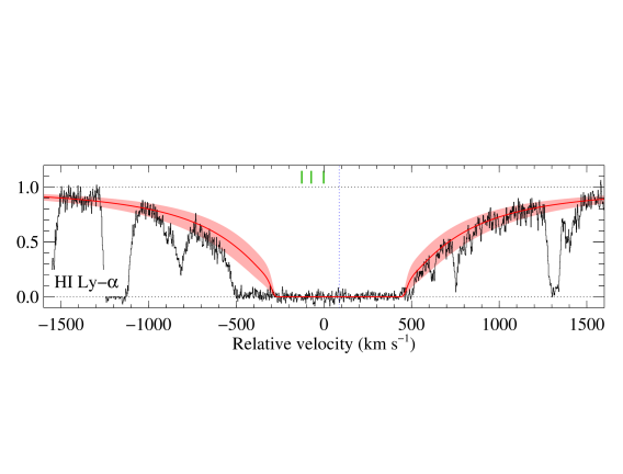
Figure 2: Measurement of the total column density of neutral atomic hydrogen at $z=2.69$ towards J 1237$+$0647. The solid line represents the best one-component fit to the data. The centroid of the profile is indicated by a dotted vertical line. Uncertainties on the column density measurement are illustrated by the shaded area. The short tick marks indicate the position of the three H₂-bearing components, the reddest of which also features CO and HD absorptions. The origin of the velocity scale, for this figure and all following ones, is defined at the position of the CO-bearing component at $z_{\rm abs}$ = 2.68957.

3.2 Metal content

3.2.1 Singly ionised species

Absorption lines from detected low ionisation species are spread over about 350 ${\rm km\,s^{-1}}$around the strongest component, which is also the component where CO and HD are detected. We used non-saturated transitions to derive accurate column densities for Fe⁺, Ni⁺, S⁺ and Zn⁺. Lines from other species (C⁺, O⁰, N⁰) are heavily saturated, preventing us to derive any meaningful value of the corresponding column densities. It is however possible to perform an accurate measurement of the Si⁺ column density from the simultaneous use of Si ii $\lambda$1808, which is very weak (below the 3 $\sigma$ detection level), and Si ii$\lambda$1304 which is close to saturation. Note that although the strong Si ii$\lambda$1304 line reveals the presence of additional weak components, their contribution to the overall column density is negligible. The result of the Voigt-profile fitting is shown on Fig. 3 with the corresponding parameters in Table 2. Both the S ii$\lambda$1253 and S ii$\lambda$1259 profiles are partially blended. Unfortunately, S ii$\lambda$1250 falls in a gap of the spectrum. Therefore, we provide only upper-limits for the blended components in Table 2. 3-$\sigma$ upper-limits on the column densities of Ni⁺ and Zn⁺ for the undetected components are provided in the table. Finally, we measure $\log N($Cr${}^{+})<12.2$ at 3 $\sigma$ from the non-detection of Cr ii$\lambda$2056.

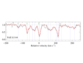
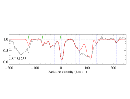
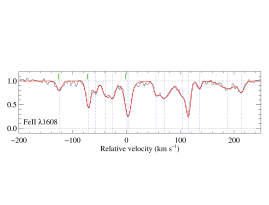
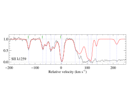
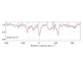
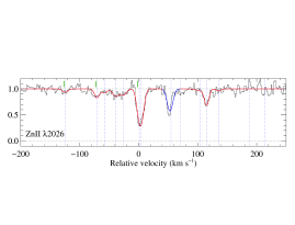
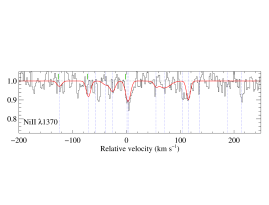
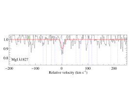
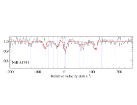
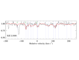
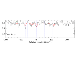
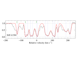
Figure 3: Fit to metal lines. The origin of the velocity scale is set at the redshift of the CO absorption ($z=2.68957$). The positions of the three H₂ components are indicated by short tick marks. The absorption seen at $v=+55\leavevmode\nobreak\ {\rm km\,s^{-1}}$ in the Zn ii$\lambda$2026 panel (in blue) is due to Mg i$\lambda$2026 while that at $v=-110\leavevmode\nobreak\ {\rm km\,s^{-1}}$ on the Si ii$\lambda$1808 panel is due to S i$\lambda 1807$. Note that both S ii lines are affected by blends. Finally Si ii$\lambda$1304 reveals the presence of additional weak components that are not fitted (see text).

Table 2: Column densities of metal species

$z_{\rm abs}$	$\Delta\,v$  (${\rm km\,s^{-1}}$)	$b$ (${\rm km\,s^{-1}}$)	$\log N$  (${\rm cm}^{-2}$)
			Fe+	Ni+	S+	Zn+	Si+	Mg0
2.68803	-125	5.2$\pm$0.2	13.03$\pm$0.06	12.18$\pm$0.13	14.03$\pm$0.02	11.46$\pm$0.15	13.82$\pm$0.02	$<$12.70
2.68870	-71	4.6$\pm$0.1	13.56$\pm$0.04	12.62$\pm$0.05	14.04$\pm$0.02	11.86$\pm$0.06	14.37$\pm$0.04	$<$12.70
2.68886	-57	4.8$\pm$0.3	13.09$\pm$0.05	$<$12.15	13.83$\pm$0.02	11.50$\pm$0.13	$\leq$13.91	$<$12.70
2.68909	-39	6.2$\pm$0.5	13.30$\pm$0.04	12.07$\pm$0.19	14.18$\pm$0.01	11.86$\pm$0.06	$\leq$14.08	$<$12.70
2.68925	-26	6.0$\pm$0.3	13.37$\pm$0.04	12.52$\pm$0.07	14.01$\pm$0.02	11.76$\pm$0.08	14.04$\pm$0.09	$<$12.70
2.68958	+1	14.5$\pm$1.5	13.41$\pm$0.05	$<$12.15	14.17$\pm$0.07	$<$11.55	13.94$\pm$0.04	$<$12.85
2.68961	+3	5.4$\pm$0.2	13.74$\pm$0.02	12.79$\pm$0.04	14.91$\pm$0.02	12.75$\pm$0.02	14.04$\pm$0.09	13.03$\pm$0.02
2.69024	+55	3.5$\pm$0.3	12.90$\pm$0.06	$<$12.15	$\leq$13.50	$<$11.40	13.21$\pm$0.08	$<$12.70
2.69044	+71	14.8$\pm$2.0	13.69$\pm$0.02	12.67$\pm$0.09	$\leq$14.70	$<$11.55	14.37$\pm$0.01	$<$12.85
2.69086	+105	9.3$\pm$2.0	13.46$\pm$0.03	$<$12.20	$\leq$14.80	11.40$\pm$0.32	14.09$\pm$0.02	$<$12.75
2.69099	+115	3.7$\pm$0.2	13.75$\pm$0.02	12.65$\pm$0.04	$\leq$14.70	12.12$\pm$0.04	14.08$\pm$0.14	$<$12.70
2.69124	+136	3.4$\pm$0.5	12.81$\pm$0.04	$<$12.15	$\leq$13.80	11.15$\pm$0.29	13.58$\pm$0.04	$<$12.70
2.69189	+188	19.5$\pm$1.7	13.40$\pm$0.03	$<$12.40	$<$13.40	$<$11.60	14.04$\pm$0.05	$<$12.95
2.69220	+214	6.5$\pm$0.5	13.12$\pm$0.03	$<$12.15	13.78$\pm$0.04	$<$11.40	13.78$\pm$0.02	$<$12.70

Total column densities and corresponding mean metallicities in the gas relative to solar are given in Table 3. Note that we do not apply ionisation correction since the presence of neutral and molecular species in the strongest components indicates the effect of ionisation on the overall abundances should be negligible. Indeed, even in the general population of absorbers, the ionisation correction is only about 0.1 dex for $N($H${}^{0})=10^{20}$ ${\rm cm}^{-2}$ (Péroux et al., 2007). The metallicity is super-solar with $[$Zn$/$H$]=+0.34$ and $[$S$/$H$]=+0.15$. Other species are depleted ([Fe/Zn] = $-$1.39, [Si/Zn] = $-$0.82). This indicates that a significant fraction of the refractory species is locked in solid phase onto dust grains. The presence of dust and its consequences are discussed in more details in Sect. 4.2.

Table 3: Summary of overall gas-phase abundances

Species	$\log N$ (${\rm cm}^{-2}$)	mean abundance
H0	20.00$\pm$0.15	$\ldots$
H2	19.21${}_{-0.12}^{+0.13}$	$\left<f_{\rm H2}\right>=0.24$
CO	14.20$\pm$0.09	$\log$ CO/H = -5.92
Zn+	13.02$\pm$0.02	[Zn/H] = +0.34$\pm$0.12
S+	15.39$\pm$0.06	[S/H] = +0.15$\pm$0.13
Fe+	14.57$\pm$0.01	[Fe/H] =-1.05$\pm$0.12
Si+	15.15$\pm$0.02	[Si/H] =-0.48$\pm$0.12
Ni+	13.48$\pm$0.03	[Ni/H] =-0.86$\pm$0.12

3.2.2 Neutral carbon

As the ionisation potential of neutral carbon (C⁰) is similar to the energy of the photons that destroy H₂, C i is usually a good tracer of the presence of H₂ (Srianand et al., 2005). The expected positions of several C i lines usually fall out of the Lyman-$\alpha$ forest. We therefore initiated a program to search for molecules along QSOs selected upon the presence of C i, as seen in the low resolution SDSS spectra. Because of this selection, it is not surprising to detect strong C i lines in the UVES spectrum of J 1237$+$0647. The profile of C i absorption lines is complex and results from the blending of absorption lines from different components seen in different excitation levels (ground state: ${}^{3}P_{0}$, first excited level: ${}^{3}P_{1}$ and second excited level: ${}^{3}P_{2}$). Nevertheless, the high signal-to-noise and high spectral resolution allow us to clearly identify eight components. Most of them are also detected in the first excited level, while only the strongest two are detected in the second excited level. The fit to C i lines is shown on Fig. 4, with the corresponding parameters given in Table 4. We considered all optically thin absorption lines but did not include in the fit weak absorption lines in the region around C i $\lambda$1277 where the placement of the continuum was uncertain. The main uncertainty in determining the C⁰ column densities comes from the uncertainties on the oscillator strengths. As in previous works from our group (e.g. Noterdaeme et al., 2007a, b; Srianand et al., 2008b) and others in the field (Jorgenson et al., 2009), we used $f$-values from Morton (2003). Using the oscillator strengths from Jenkins & Tripp (2001) results in 2 to 3 times lower column densities.

The relative populations of the fine-structure levels of neutral carbon depend on the gas pressure. Since the kinetic temperature of the gas can be derived from the the relative populations of the low rotational levels of H₂ (see Sect. 3.3), it is possible to measure the volumic density of the gas. From figure 2 of Silva & Viegas 2002 (see also Srianand et al., 2000) and taking into account excitation by collisions and by the Cosmic Microwave Background radiation, we can see that the measured ratios $\log N($C⁰,J=1)/$N($C⁰,J=0) = $-$0.2 and $\log N($C⁰,J=2)/$N($C⁰,J=0) = $-1$ in the main component, coinciding with the position of the CO component, correspond to a volumic density of the order of $n_{\rm H^{0}}\sim 50$-60 cm^-3 for $T\sim 110$ K (see Sect. 3.3). Other components have similar fine-structure ratios, which indicate similar thermal pressure. The kinetic temperature is probably larger in all other components (which is verified at least for the two other H₂-bearing components, see Table 6), implying smaller densities (e.g. $n_{\rm H^{0}}\sim$ 1-10 cm^-3 in the component at $v=$ -127$\leavevmode\nobreak\ {\rm km\,s^{-1}}$).

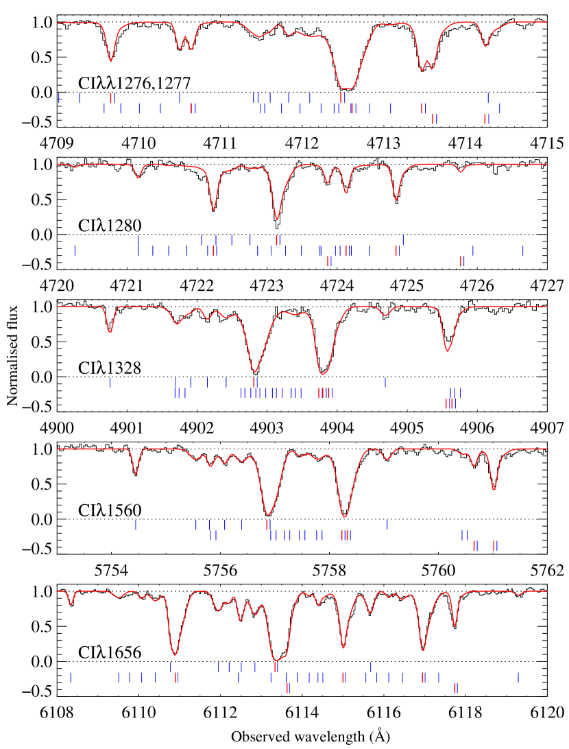
Figure 4: Portions of the J 1237$+$0647 UVES spectrum around C i absorption lines. The short vertical marks in each panel represent the positions of absorption lines from the ground state (${}^{3}P_{0}$), the first excited level (${}^{3}P_{1}$) and the second excited level (${}^{3}P_{2}$) from top to bottom, respectively. The component where CO is detected (at $z_{\rm abs}$ = 2.68957) is marked in red.

Table 4: Column densities of neutral carbon in fine-structure levels

$z_{\rm abs}$	$\Delta\,v$	$b$	$\log N($C0) (${\rm cm}^{-2}$)
	(${\rm km\,s^{-1}}$)	(${\rm km\,s^{-1}}$)	${}^{3}P_{0}$	${}^{3}P_{1}$	${}^{3}P_{2}$	total
2.68802	-126	1.2$\pm$0.1	13.24$\pm$0.04	12.80$\pm$0.03		13.37$\pm$0.03
2.68872	-69	11.8$\pm$0.6	12.84$\pm$0.03	12.70$\pm$0.05		13.08$\pm$0.02
2.68888	-56	3.3$\pm$1.3	12.37$\pm$0.08			12.37$\pm$0.08
2.68906	-41	3.0$\pm$0.4	12.82$\pm$0.02	12.56$\pm$0.04		13.01$\pm$0.02
2.68926	-25	7.4$\pm$0.4	12.94$\pm$0.02	12.87$\pm$0.02		13.21$\pm$0.01
2.68956	-1	1.4$\pm$0.1	14.67$\pm$0.04	14.46$\pm$0.03	13.64$\pm$0.02	14.90$\pm$0.03
2.68960	+2	8.8$\pm$0.1	13.98$\pm$0.01	13.79$\pm$0.01	12.98$\pm$0.03	14.22$\pm$0.01
2.69097	+114	3.6$\pm$0.5	12.70$\pm$0.02	12.42$\pm$0.08		12.88$\pm$0.03

3.2.3 Neutral sulphur

The first ionisation potential of sulphur being of 10.36 eV, this element is hence usually observed in its first ionised state (S⁺) in Damped Lyman-$\alpha$ systems. In turn, sulphur is expected to be found in neutral form (S⁰) inside molecular clouds, where the surrounding UV field has been strongly attenuated. To date, S⁰ has been detected only in QSO absorbers where CO absorption is seen as well: in the systems at $z$=2.42 towards SDSS J143912.04$+$111740.5 (hereafter J 1439$+$1117; Srianand et al., 2008b) and at $z$=1.64 towards SDSS J160457.50$+$220300.5 (Noterdaeme et al., 2009a).

Absorption lines from eight transitions of neutral sulphur are detected in the UVES spectrum of J 1237$+$0647. This strengthens the claim that the presence of neutral sulphur flags molecular gas. Just like the presence of neutral carbon is a good indicator of that of H₂ (Srianand et al. 2005, albeit with generally modest molecular fractions, Noterdaeme et al. 2008a), S i lines might well indicate the presence of CO. This is however of little practical use for pre-selecting CO-bearing DLAs from the low resolution SDSS spectra, since S i and CO lines are located in the same spectral region and have similar strengths.

We used all detected S i lines to constrain the column density and $b$ parameter. Two components are needed to properly fit the data, with resulting $\chi^{2}_{\nu}\simeq 1$. The $b$-value obtained is less than 1 ${\rm km\,s^{-1}}$ for the main component, i.e., well below the spectral resolution ($\sim$6 ${\rm km\,s^{-1}}$). However, $b$ is well constrained, thanks to the relatively large range spanned by the oscillator strength values. However, the fit is sensitive to the exact value of the spectral resolution. Therefore, to add confidence to the $b$ and $N$ measurements, we built the curve of growth for the detected S i lines, which does not depend on the spectral resolution (see Fig. 6). The error on the equivalent width measurements are conservative and take into account uncertainties in the continuum placement. From this figure, we confirm the small Doppler parameter. The measured column density nicely matches the sum of the individual column densities in the two components derived from the Voigt-profile fitting.

Table 5: S⁰ column densities

$z_{\rm abs}$	$\Delta\,v$  (${\rm km\,s^{-1}}$)	$\log N($S0) (${\rm cm}^{-2}$)	$b$ (km s-1)
2.68953	-3	12.29$\pm$0.06	1.1$\pm$0.5
2.68958	+1	13.19$\pm$0.04	0.7$\pm$0.1

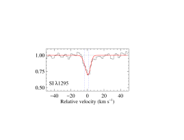
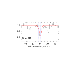
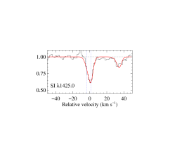
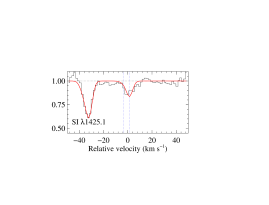
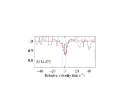
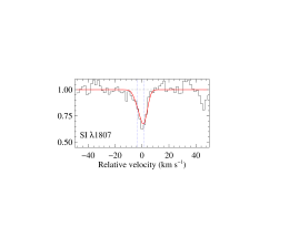
Figure 5: Fit to S i absorption lines. Results of the best model fit using two components is overplotted ($\chi^{2}_{\nu}=0.97$).

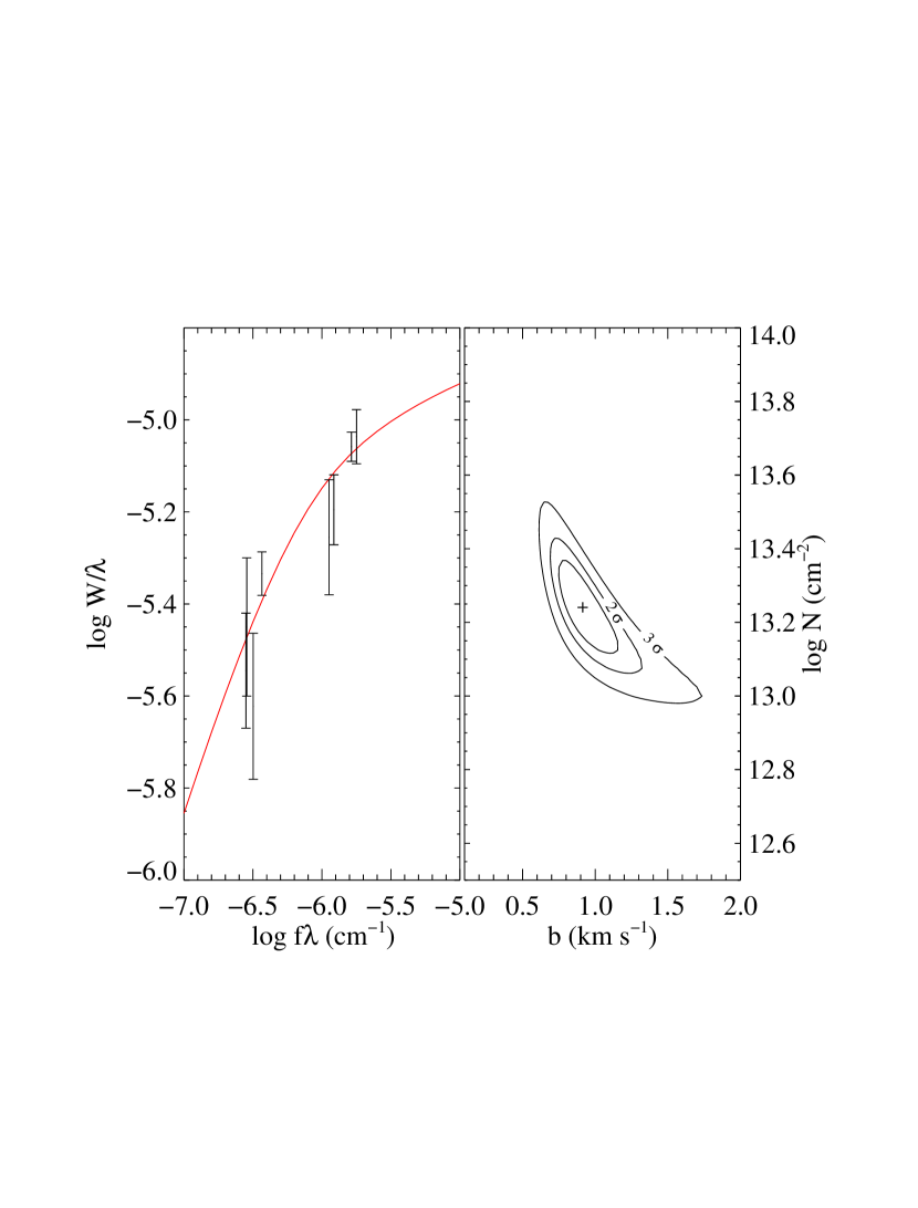
Figure 6: Curve of growth analysis of S i absorption lines. Left: Curve of growth. Right: confidence interval. Minimum $\chi^{2}_{\nu}$ (0.91) is reached for $\log N($S${}^{0})=13.24$, $b=0.91$ ${\rm km\,s^{-1}}$.

3.2.4 Neutral chlorine

Chlorine, with an ionisation potential of 12.97 eV is a unique species among those that can be photoionised by photons with energy $h\nu<13.6$ eV. The dominant form of chlorine is Cl⁺ when hydrogen is mostly in the atomic form. However, neutral chlorine (Cl⁰) results from rapid exothermic ion-molecule reaction between singly-ionised chlorine (Cl⁺) and H₂ when H₂ is optically thick (Jura, 1974). Therefore, the presence of neutral chlorine in the ISM is expected to be a good indicator of the presence of molecular gas.

Cl⁰ is clearly detected at $z_{\rm abs}$ = 2.689560, associated with the strongest H₂ component. We measure $\log N$(Cl⁰) = 13.01$\pm$0.02 from the fit to the Cl i$\lambda$1347 absorption line, with $b=4.5\pm 0.4$ ${\rm km\,s^{-1}}$ (see Fig 7). From the non-detection of Cl ii$\lambda$1071, we derive $\log N$(Cl${}^{+})<13.4$ at the 3 $\sigma$ confidence level, which translates to $f_{\rm Cl^{0}}\equiv N$(Cl${}^{0})/(N$(Cl${}^{0})+N$(Cl${}^{+}))>0.3$. As the fraction of chlorine in neutral form is expected to follow approximately that of hydrogen in molecular form (Jura & York 1978, see also Sonnentrucker et al. 2002), the lower limit on $f_{\rm Cl^{0}}$ indicates that hydrogen could be mostly molecular at the place where we detect Cl⁰. We indeed show in the next Section that the molecular fraction is particularly high in this component.

Figure 7: Cl i$\lambda$1347 absorption at $z_{\rm abs}$ = 2.68960. A single component fit is overplotted.

3.3 Molecular hydrogen

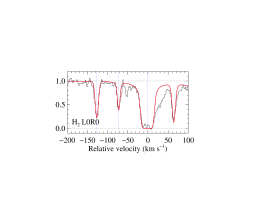
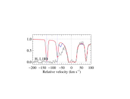
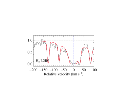
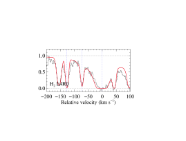
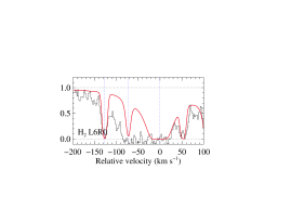
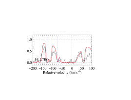
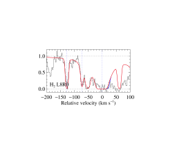
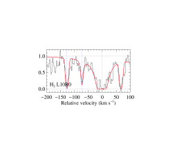
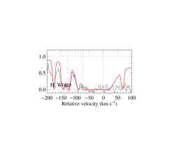
Figure 16: Fit to H₂(J=0) lines. The blue profile is the contribution from HD.

Molecular hydrogen is detected in three components at $z_{\rm abs}$ = 2.68801, 2.68868 and 2.68955, spread over $\sim$ 125 km s^-1. The strongest component at $z_{\rm abs}$ = 2.68955 also features HD and CO absorption lines. The UVES spectrum covers numerous Lyman bands (B${}^{1}{\Sigma_{u}}^{+}\leftarrow$ X${}^{1}{\Sigma_{g}}^{+}$) as well as some Werner bands (C${}^{1}{\Pi_{u}}^{+}\leftarrow$ X${}^{1}{\Sigma_{g}}^{+}$), which allows for an accurate measurement of the H₂ column densities in each component and in different rotational levels. A portion of the UVES spectrum covering the H₂ Lyman (1-0) band is shown on Fig. 8, while the full velocity plots for different rotational levels are shown on Figs. 16 to 21. The measured column densities and corresponding excitation temperatures are given in Table 6). In the following, we refer to these components as #1, #2 and #3 from the bluest to the reddest.

Component #1 has similar width in all rotational levels and requires a single Doppler parameter to describe the profiles of the H₂ J=0 to J=3 absorption lines. The Doppler parameter ($b\sim 3$ ${\rm km\,s^{-1}}$) is likely to be dominated by turbulent motions.

Component #2 presents a broadening of the profiles with increasing rotational level and requires different Doppler parameters. This behaviour has already been observed in the Galactic ISM (e.g. Jenkins & Peimbert, 1997; Lacour et al., 2005b) but also in high redshift Damped Lyman-$\alpha$ systems (Noterdaeme et al., 2007a). Doppler parameters can be measured accurately even when significantly smaller than the spectral resolution thanks to the presence of numerous transitions with different oscillator strengths. However, the measurement of $b$ in the first rotational level (J = 0) remains difficult due to the small number of unblended absorption lines (see Table 6). However, there are enough transitions from the J = 0 and 1 levels together to ascertain the fact that the Doppler parameter of the transitions from these two levels is very small, of the order of $b\sim 1$ ${\rm km\,s^{-1}}$. This is consistent with thermal excitation with a temperature of $T_{\rm k}\sim$ 120 K, which is similar to what is measured from $T_{\rm 01}$.

The reddest component (#3) is very strong, with damping wings seen for rotational levels up to J = 3, allowing for accurate measurement of the column densities. Non-saturated lines for J = 4 and 5 also allow for accurate measurements in these rotational levels. Component #3 is particularly interesting not only because of its large H₂ column density, but because it also contains deuterated molecular hydrogen, carbon monoxide as well as neutral sulphur and neutral chlorine, all of which have been very rarely detected at high redshift. Since the column density of H₂ is large, the J = 0 and J = 1 levels are self-shielded and the collisional time-scale is much shorter than the photo-dissociation time-scale. Therefore, the $N$(J=1)/$N$(J=0) ratio is maintained at the Boltzmann equilibrium value. This means that the measurement of the kinetic temperature from $T_{01}$ is robust. We measure $T_{01}$ = $T_{\rm kin}$ $\sim$ 110 K, which is similar to the temperature in the local interstellar medium ($T_{\rm kin}$ $\sim$ 80 K; Savage et al., 1977).

We measure a total column density $\log N($H${}_{2})=19.21_{-0.12}^{+0.13}$ in the sub-DLA system with far the most important contribution coming from the CO-bearing component (component #3). This corresponds to a large mean molecular fraction $\left<f_{\rm H2}\right>=2N(\mbox{H${}_{2}$})/(2N(\mbox{H${}_{2}$})+N({\rm H}^{0}))=0.24^{+0.13}_{-0.08}$. However, the centre of the H i Lyman-$\alpha$ absorption line is clearly shifted from component #3 by more than 50 km s^-1 (see Fig. 2). This means that the amount of atomic hydrogen in the CO-bearing cloud is much smaller than $\log N($H${}^{0})=20$ and the value given above should be considered as a lower limit on the actual molecular fraction in the CO-bearing cloud (i.e. $f_{\rm H2}>1/4$). As noticed in the previous section from the presence of Cl⁰ absorption associated with #3, the molecular fraction in the component #3 is probably not far from unity.

Table 6: H₂ column densities and excitation temperatures

component	$\log N$(H2,J)	$b$	$T_{\rm 0-J}$
$z_{\rm abs}$, $v$ (${\rm km\,s^{-1}}$)	(${\rm cm}^{-2}$)	(${\rm km\,s^{-1}}$)	(K)
#1, $z$=2.68801, $\Delta\,v$=-127	16.28${}_{-0.10}^{+0.10}$
J=0	15.51$\pm$0.05	3.3$\pm$0.2	–
J=1	16.08$\pm$0.10	”	193${}_{-54}^{+123}$
J=2	15.39$\pm$0.20	”	271${}_{-63}^{+120}$
J=3	15.13$\pm$0.05	”	261${}_{-15}^{+16}$
#2, $z$=2.68868, $\Delta\,v$=-73	17.62${}_{-0.11}^{+0.08}$
J=0	16.94${}_{-0.44}^{+0.20}$	0.4${}_{-0.1}^{+0.8}$	–
J=1	17.51$\pm$0.05	1.2$\pm$0.1	$\geq 117$
J=2	15.25$\pm$0.03	3.3$\pm$0.2	93${}_{-9}^{+20}$
J=3	14.89$\pm$0.02	4.9$\pm$0.2	131${}_{-8}^{+19}$
#3, $z$=2.68955, $\Delta\,v$=-2	19.20${}_{-0.12}^{+0.13}$
J=0	18.65$\pm$0.20	6.0$\pm$0.1	–
J=1	18.92$\pm$0.10	”	108${}_{-33}^{+84}$
J=2	18.18$\pm$0.10	”	190${}_{-39}^{+66}$
J=3	18.21$\pm$0.10	”	252${}_{-36}^{+52}$
J=4	15.43$\pm$0.10	7.9$\pm$0.1	177${}_{-11}^{+14}$
J=5	14.95$\pm$0.05	”	213${}_{-10}^{+11}$

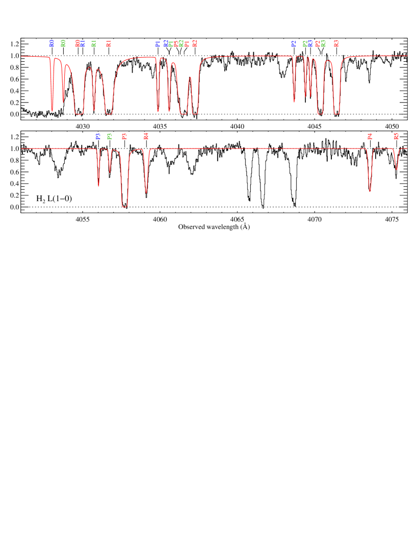
Figure 8: Portion of the UVES spectrum of J 1237$+$0647 covering the (1-0) Lyman band of H₂. The labels indicate the branches (’R’, ’P’ for $\Delta J=-1,+1$, respectively) and the rotational levels of the lower states. Absorptions from different components are indicated using different label colours (#1: blue, #2: green, #3: red).

3.4 HD and the D/H ratio

Several Lyman-band HD lines from the first two rotational levels are detected in the UVES spectrum (see Fig. 9). Unfortunately, J = 1 lines are either severely blended or redshifted in regions of bad signal-to-noise ratio and we can only derive an upper limit on the column density for this rotational level. We measure the HD column density in the J=0 rotational levelx from fitting the HD L5R0 and HD L8R0 lines which are unblended. Measurements are summarised in Table 7.

We measure $N(\mbox{HD})/2N(\mbox{H${}_{2}$})=0.95\times 10^{-5}$. This is about 10 times higher than what is measured in the Galactic ISM (Lacour et al., 2005a) for $f=0.24$. Since this ratio is known to increase with the molecular fraction (Lacour et al., 2005a) HD/2H₂ might provide a lower limit on D/H for $f_{\rm H2}<1$. If, as discussed previously, the actual molecular fraction in the HD-bearing cloud towards J 1237$+$0647 is higher than 0.25, both HD and H₂ could be self-shielded and $\mbox{HD}/2\mbox{H${}_{2}$}$ $\sim$ D${}^{0}/$H⁰. The value we obtain is then consistent with the D${}^{0}/$H⁰ ratio measured in the Galactic disc (Linsky et al., 2006). This corresponds to an astration factor of $\sim$3 when comparing to the primordial value as measured in low-metallicity absorption systems (D/H = 2.82$\pm$0.2$\times$10^-5; Pettini et al. 2008, Ivanchik et al. 2010, see however Srianand et al. 2010) or derived from the baryon density parameter (Steigman, 2007).

Note that all five high redshift HD detections to date yield relatively large D/H values despite significant metal enrichment: $N(\mbox{HD})/2N(\mbox{H${}_{2}$})=1.5\times 10^{-5}$, $3.6\times 10^{-5}$, $7.9\times 10^{-5}$ and $1.6\times 10^{-5}$ towards respectively, J 1439$+$1117 (Noterdaeme et al., 2008b), Q 1232$+$082 (Ivanchik et al., 2010), J 2123-0500 and FJ 0812+32 (Tumlinson et al., 2010). Since deuterium is easily destroyed as interstellar gas is cycled through stars, large deuterium abundances are difficult to reproduce with closed-box models. However, these are well explained by models including infall of primordial gas (e.g. Prodanović & Fields, 2008). If the velocity-metallicity correlation found by Ledoux et al. (2006a) is the consequence of an underlying mass-metallicity relation, then we can expect that a high astration of deuterium in high metallicity systems is roughly compensated by a strong infall of primordial material onto massive galaxies. However, Tumlinson et al. (2010) noted that HD/2H₂ ratios in high-$z$ absorption systems lie in a narrow range well above the value measured in the Galaxy while these systems present a large diversity in terms of metallicities and molecular fractions. This puzzling behaviour led them to conclude that it could be premature to use the HD/2H₂ ratio to derive $\Omega_{b}$, given our actual understanding of interstellar chemistry. In addition, we note that in the case of QSO absorbers, we only have access to the properties of the gas (metallicities, molecular fractions) averaged over the line of sight. These may not be representative of the actual chemical abundances in the HD-bearing cloud. Indeed, only the total $N($H⁰) can usually be measured and the metal components are blended into a smooth absorption profile. It is therefore necessary to be careful and to study each system in detail (e.g. Balashev et al., submitted) to derive the local chemical and physical conditions in the cloud.

Table 7: HD column densities

component	$\log N$(HD,J) (${\rm cm}^{-2}$)	$b$ (${\rm km\,s^{-1}}$)
$z_{\rm abs}$=2.68956, $\Delta\,v$=-1 ${\rm km\,s^{-1}}$
J=0	14.48$\pm 0.05$	4.5$\pm$0.2
J=1	$\leq 13.60$	”

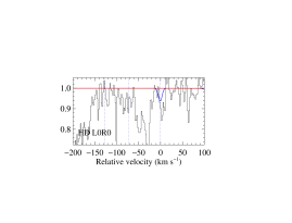
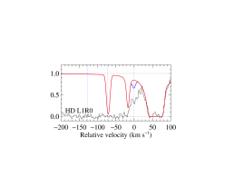
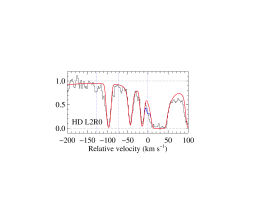
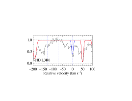
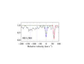
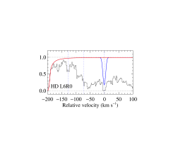
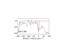
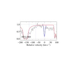
Figure 9: Fit to HD J=0 lines. The blue profile is the contribution from HD while the red profile represents H₂. The velocity of the H₂ detected components are indicated by vertical dotted lines.

3.5 Carbon monoxide

Absorptions from eight $A^{1}\Pi(\nu^{\prime})\leftarrow X^{1}\Sigma^{+}(\nu$=$0)$ bands of CO (from $AX$ (0-0) to $AX$ (7-0)), the $C^{1}\Sigma(\nu^{\prime}$=$0)\leftarrow X^{1}\Sigma^{+}(\nu$=$0)$ Rydberg band and the $d^{3}\Delta(\nu^{\prime}$=$5)\leftarrow X^{1}\Sigma^{+}(\nu$=$0)$ inter-band system are detected at $z_{\rm abs}$ = 2.68957 towards J 1237$+$0647, see Fig. 10. Each band produces a complex absorption profile which results from superposition of absorption lines from different rotational levels in the P and R branches. The resolving power ($R\sim$ 50 000) and the signal-to-noise ratio (SNR $\sim$ 28) of the UVES spectrum are high enough to individually measure the column densities in rotational levels up to J = 3. In addition, the J = 4 level is probably detected in the P branch of $CX$ (0-0). We use the $AX$ and $dX$ bands that fall outside of the Lyman-$\alpha$ forest to measure the column densities in rotational levels up to J = 3. The $AX$ (3-0) band is affected by a spike likely due to a cosmic ray impact at the position of the R branch and this region is therefore not considered when fitting the profile. In addition, we use the $CX$(0-0) band up to J = 4. This band is the strongest one available but the corresponding rest wavelength (1088 Å) makes it redshifted in the Ly-$\alpha$ forest. Fortunately, only the R branch is blended whereas the P branch is free from any blend. Moreover, the $CX$ rotational levels are well separated at the UVES spectral resolution.

The results of the fit are presented in Table 8. Two errors are quoted in this table for the column densities: the first one is the rms error on the fit, while the second one reflects the uncertainties resulting from the continuum placement. The latter uncertainties were estimated by changing the normalisation by plus or minus 0.5 $\sigma$ (i.e. about $\pm$ 2% for SNR = 28) around the best continuum fit. The total CO column density we derive is $\log N($CO) = 14.17$\pm$0.09, implying a high CO to H₂ ratio of $N$(CO)/$N($H${}_{2})=10^{-5}$. This is typical of what is seen in translucent clouds (see Burgh et al., 2010).

Table 8: CO column densities and excitation temperatures

component	$\log N($CO,J)	$b$ (${\rm km\,s^{-1}}$)	$T_{\rm 0-J}$ (K)
$z_{\rm abs}=2.68957$	14.17$\pm$0.09	0.9$\pm$0.1
J=0	13.53$\pm$0.04$\pm$0.08	”	–
J=1	13.77$\pm$0.02$\pm$0.07	”	10.1${}_{-2.0}^{+4.3}$
J=2	13.54$\pm$0.03$\pm$0.06	”	10.5${}_{-1.1}^{+1.4}$
J=3	13.21$\pm$0.04$\pm$0.09	”	12.4${}_{-0.9}^{+1.0}$
J=4	12.64$\pm$0.16$\pm$0.11	”	13.0${}_{-1.6}^{+1.9}$

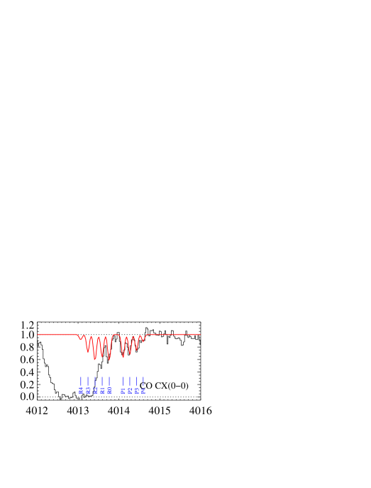
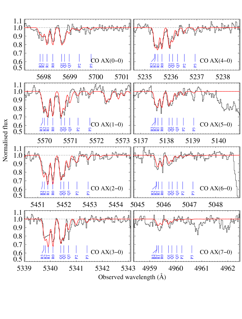
Figure 10: Fit to CO lines ($\chi^{2}_{\nu}=1.1$). The additional absorption seen in the CO AX(1-0) panel is due to the CO dX(5-0) inter-band system. Short vertical lines indicate the branch (’R’, ’P’ or ’Q’) and the rotational level of the transition.

In Fig. 11, we show the excitation diagram of CO. It is clear that the population of the first three rotational levels can be reproduced with a single excitation temperature. We measure this excitation temperature by performing a linear fit of $\log N($CO,J$)/g_{\rm J}$ vs the energy of the levels ($E_{\rm 0J}$). The fit and 1 $\sigma$ range on Fig. 11 corresponds to the best fit continuum. In order to estimate the effect of the continuum placement, we repeat the linear fit for each set of continua and take the extrema as representative of the range of possible values for $T_{\rm ex}$(CO). This gives $T_{\rm ex}=10.5^{+0.8}_{-0.6}$. Note that the effect of the continuum placement is mainly a change in the total CO column density, while little change on the slope of the linear fit (i.e. the excitation temperature). The CO excitation temperature is well below the kinetic temperature of the gas. This means that the gas density is small enough so that radiative processes are likely to dominate the downwards cascade, as predicted in diffuse molecular and translucent clouds (e.g. Warin et al., 1996). Indeed, the population ratios of the neutral carbon fine-structure levels, indicate a volumic density of the order of $n_{\rm H^{0}}\sim 50$ cm^-3, well below the critical density at which the collisional de-excitation rate of CO(J=1-0) equals that of the spontaneous emission ($n_{\rm crit}\sim$ 1000 cm^-3; Snow & McCall, 2006). Indeed, in terms of density and molecular fraction, the CO-bearing system presented here is very similar to that presented in Srianand et al. (2008b) where we concluded that collisional excitation of CO is negligible. It is important to note however, that the fine-structure levels of C⁰ only give the average volumic density. The actual local volumic density in the CO-bearing cloud could be higher. A small shift ($\sim$ 1 ${\rm km\,s^{-1}}$) is measured between the strongest C i feature and the CO component. This may indicate that the two species are not completely co-spatial.

From the radiative code RADEX (van der Tak et al., 2007), we expect the excitation temperature of CO to be about one degree larger than the expected temperature of the Cosmic Microwave Background (CMB) radiation ($T_{\rm CMB}(z$=$2.69)=10.05$ K) as soon as the collision partner (H⁰, H₂ and He) density is larger than 50 cm^-3. This explains that the excitation temperature we measure is slightly higher than what is expected from excitation by the CMB radiation alone.

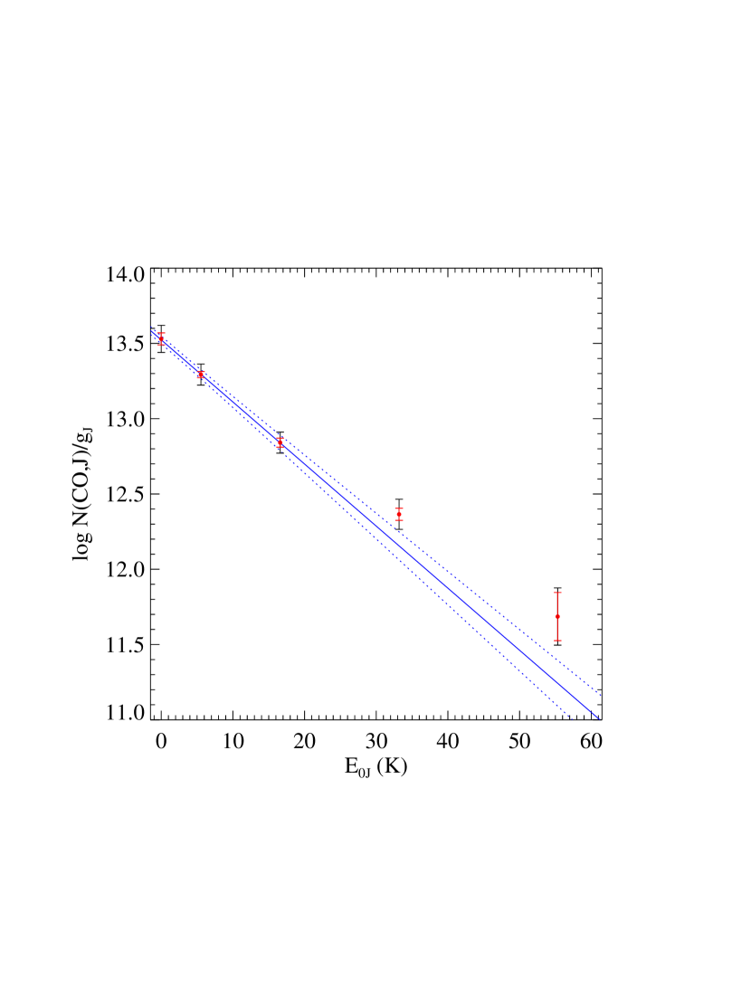
Figure 11: Excitation diagram of CO rotational levels. Errors on the column densities from fitting the lines are represented by the small red error bars while the long black error bars take into account the uncertainty in the continuum placement. The plain line represents the linear regression fit using J = 0 to J = 2 measurements and the best continuum fit. 1 $\sigma$ errors are represented by dashed lines.

In Fig. 12, we compare the excitation temperature of CO at high redshift with that in the local Universe. In the local ISM, the temperature is seen a few degrees above $T_{\rm CMB}$ at low CO column densities and rises for column densities above $N$(CO)$=2\times 10^{15}$ ${\rm cm}^{-2}$. This is due to the increased importance of photon trapping at larger column densities (Burgh et al., 2007). The values observed at high redshift are significantly higher than the local ones, despite similar $N$(CO) and kinetic temperatures. This clearly means that the main physical difference between high redshift and local lines of sight is the higher CMB temperature at high redshift. This provides a strong positive test to the hot Big-Bang theory. Another consequence of Fig. 12 is that only CO-bearing systems with $\log N($CO$)<15$ – for which there is no correlation between $N($CO) and $T_{\rm ex}$(CO) – are good places where to measure the evolution of $T_{\rm CMB}$ with cosmic time.

Interestingly, although the differences are small and within errors, we measure a systematic trend, $T_{04}\ga T_{03}\ga T_{02}\ga T_{01}$, regardless of the exact continuum placement. This indicates that while CMB photons dominate the rotational excitation of CO, other mechanisms are at play. We fail to reproduce the increasing temperature with increasing rotational level with RADEX. However, such behaviour has already been noticed in the local ISM (Sonnentrucker et al., 2007; Sheffer et al., 2008) and could be explained by the selective self-shielding of low rotational lines for $\log N$(CO)$>$14 (Warin et al., 1996). The self-shielding of far-UV Rydberg bands of CO (those relevant to the photo-destruction process) could be more effective than previously thought (Sheffer et al., 2003). In addition, the presence of H₂ lines in the same spectral region can contribute to an effective shielding of CO lines. Finally, radiative pumping from CO emission lines due to nearby dense molecular clouds could contribute to populate the higher rotational levels in the absorbing cloud (Wannier et al., 1997). If the increasing temperature with increasing rotational level is physical, then $T_{01}=10.1^{+4.3}_{-2.0}$ K could represent better the excitation by the CMB alone.

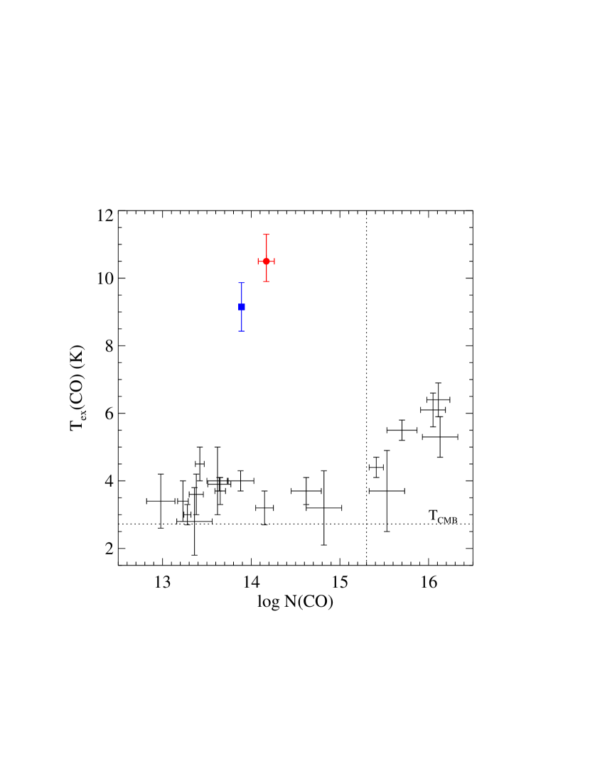
Figure 12: Excitation temperature of CO as a function of the total CO column density. Black error bars are measurements at $z=0$ from Burgh et al. (2007). The red filled circle with error bars is our measurement at $z=2.7$ towards J 1237$+$0647 while the blue square represents the measurement at $z=2.4$ towards J 1439$+$1117 (Srianand et al., 2008b). Only a large range on $T_{\rm ex}$ (6-16 K) could be determined for the system at $z=1.64$ towards SDSS J160457.50$+$220300.5 (Noterdaeme et al., 2009a), and is therefore not represented in the figure. The vertical dotted line is indicative of a change of behaviour: below this limit there is no correlation between $N($CO) and $T_{\rm ex}$(CO).

4 The nature of the absorbing cloud

4.1 Summary of the physical properties in the CO component

In the previous sections, we have derived physical properties of the gas associated to the molecular absorptions seen at $z_{\rm abs}$ $\sim$ 2.68957 towards J 1237$+$0647.

From the analysis of Cl⁰, we derived that the molecular fraction, 2$N$(H₂)/(2$N$(H₂)+$N$(H⁰)), in the CO component is larger than 1/4 for a super-solar metallicity: $Z$(Zn,S) = +0.34,+0.15. From the populations of the C⁰ ground-state fine structure levels, we found that the particle density is of the order of $\sim$50 cm^-3. The analysis of the H₂ rotational levels yields a kinetic temperature of $\sim$100 K and CO is mainly excited by radiative interaction with the CMBR.

We can have an indication of the electronic density in the cloud thanks to the S⁰/S⁺ ratio. Assuming that the mean ratio can be derived using the column densities in the strongest components we measure: $\log N$(S⁰)/$N($S${}^{+})$ = $-1.72$. The electronic density, $n_{\rm e}$, is derived from the ionisation equilibrium between the two species

$$\Gamma n({\rm S}^{0})=\alpha n_{\rm e}n({\rm S}^{+}),$$ (1)

where $\Gamma$ is the photoionisation rate of S⁰ and $\alpha$ the combination rate of S⁺. Taking the ratio in diffuse gas of the Galaxy ($\Gamma/\alpha$ $\sim$ 95 cm^-3, Péquignot & Aldrovandi 1986; see also table 8 of Welty et al. 1999b) we derive $n_{\rm e}$ $\sim$ 1.85 ($\Gamma/\alpha$/95) cm^-3. Note that this is an average value in the strongest metal component. Since S⁰ and S⁺ are not co-spatial –as indicated by the different Doppler-parameters– the electron density derived here should be considered as an upper limit in the molecular gas.

We could apply the same reasoning to carbon but we cannot measure the C⁺ column density as C ii$\lambda$1334 is highly saturated. In turn we can derive $N$(C⁺) from the sulphur electronic density measurement. We find

$${{N({\rm C}^{+})}\over{N({\rm S}^{+})}}={{\Gamma({\rm C}^{0})/\alpha({\rm C}^{+})}\over{\Gamma({\rm S}^{0})/\alpha({\rm S}^{+})}}{{N({\rm C}^{0})}\over{N({\rm S}^{0})}}$$ (2)

Using $\Gamma($C${}^{0})/\alpha$(C⁺) = 32 cm^-3 yields $\log N$(C⁺)/$N$(S⁺) = $1.26$ which is close to the solar ratio.

4.2 Dust content

Fig. 13 shows the distribution of $g-r$ colours for 650 non-BAL quasars with redshifts similar to J 1237$+$0647  ($\Delta z=0.1$). The median $g-r$ value of the distribution is 0.16 with a standard deviation of 0.11. This dispersion reflects the color variation from one QSO to the other and is not due uncertainties in the SDSS photometric measurements (which are better than 0.03 mag). This implies that the colour excess of J 1237$+$0647 ($g-r=0.59$) is significant at the 3.9 $\sigma$ level. This significance increases to 4.9 $\sigma$ if we consider a Gaussian fit to the distribution. Indeed, there is a tail towards large colour excesses which shows the existence of a population of reddened quasars. J 1237$+$0647 is among the reddest 1.5% quasars having $g-r>0.5$.

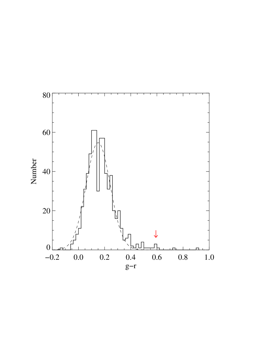
Figure 13: Distribution of SDSS photometric $g-r$ values for a sample of 650 non-BAL QSOs at $2.681<z<2.881$. The arrow indicates the position of J 1237$+$0647.

The observed flux-calibrated SDSS spectrum of J 1237$+$0647 is matched by the QSO composite spectrum from Vanden Berk et al. (2001) reddened by a SMC-like extinction law with E(B-V) = 0.05$\pm$0.01. The spectrum together with the fit is shown in Fig. 14. Note that since we are only interested in the slope of the continuum of J 1237$+$0647 and the strength of emission lines varies strongly from one quasar to the other, we do not include emission line regions in our fit. Absorption lines were also ignored during the fit as well as the wavelength range bluewards of the Ly-$\alpha$ emission.

In order to further estimate the probability that the above reddening might be due to a peculiar intrinsic QSO shape, we used a technique described in (Srianand et al., 2008a; Noterdaeme et al., 2009a): We repeated the spectral slope fitting assuming an absorber at $z=2.69$ for a control sample of 82 non-BAL QSOs with similar emission redshifts ($2.76<z_{\rm em}<2.80$) and spectra with $i$-band S/N ratios larger than 5. We find that the continuum slope of J 1237$+$0647 deviates at the 98% confidence level from the mean slope of other quasars. In the following, we will therefore consider that the colour excess of J 1237$+$0647 is due to the presence of dust at $z_{\rm abs}=2.69$.

Our best-fit model predicts J = 16.9, H = 16.3, K = 15.5 (with typical errors of 0.2 mag), while the observed Two Micron All Sky Survey (2MASS) magnitudes are J = 16.8$\pm$0.2, H = 15.7$\pm$0.2, and K $>$ 15.0. The agreement although not perfect in the H-band is reasonable. Indeed, the 2MASS magnitudes come from Point Source Reject Table for objects with very low SNR. These measurements are known to suffer from flux overestimation which can easily explain the discrepancy between predicted and measured H-band magnitudes. In addition, the presence of the H-$\beta$ emission line in the H-band increases the uncertainty of our estimate. This together with the fact that the 2MASS and SDSS observations were taken five years apart, makes our predicted magnitudes consistent with the 2MASS data. Unfortunately, there are no SDSS measurements at different epochs for this object to monitor any variation in the QSO flux.

The measured reddening, although significative, is marginally higher to what is seen in the general population of DLAs (E(B-V) $\sim 0.04$, Ellison et al. 2005). Interestingly, the integrated extinction-to-gas ratio measured towards J 1237$+$0647, A(V)/$N$(H${}^{0})$ = 1.5$\times 10^{-21}$ mag cm² is 20 times higher that the average value for the SMC (7.5$\times 10^{-23}$ mag cm²; Gordon et al., 2003) and about 50 times higher than the mean value measured in high redshift DLAs (2-4$\times 10^{-23}$ mag cm²; Vladilo et al., 2008). This means that would the H⁰ column density have been higher, the extinction induced would have been so large that the QSO would have been missed by the SDSS target selection. Note that the moderate extinction $A_{\rm V}=0.14$ in the rest-frame of the absorber, already produces an extinction of nearly 1 mag in the $g$-band. This supports further the possibility that current surveys can miss a large number of cold clouds (Noterdaeme et al., 2009a). If, as discussed before, a large fraction of the atomic hydrogen is not associated with the molecular component, then the extinction-to-gas ratio in the molecular component is even higher. The line-of-sight to J 1237$+$0647 probably passes through a relatively thin slab of dusty gas. This is also supported by the high depletion factors measured in the CO-bearing component ([Fe/Zn]$\sim$-2.0, [Ni/Zn]$\sim$-1.6, [Si/Zn]$\sim$-1.7, [Cr/Zn] $<-1.6$). Such abundance pattern is typical of what is seen in cold gas of the Galactic disk (Welty et al., 1999a).

If we consider the extinction only, then the sightline studied in this paper is not translucent. Indeed, the historical definition of translucent corresponds to 1 $<$ $A_{\rm V}$ $<$ 5. However, as noted by Rachford et al. (2002), even translucent sightlines can result from the concatenation of multiple diffuse clouds along the line-of-sight. This kind of scenario has already been advocated to explain the bimodal distribution in the $\log N$(H${}_{2})$ distribution for a given column density of dust (Noterdaeme et al., 2008a). Therefore extinction may not be the best parameter to define translucent clouds. Rachford et al. (2002) and Snow & McCall (2006) have proposed that the definition of translucent clouds should be based on the local properties of the gas rather than the integrated properties along the line-of-sight. Following this suggestion, Burgh et al. (2010) have presented a definition based on the abundance of hydrogen and carbon in molecular forms. These authors noted that with this definition, translucent clouds do not produce necessarily strong reddening.

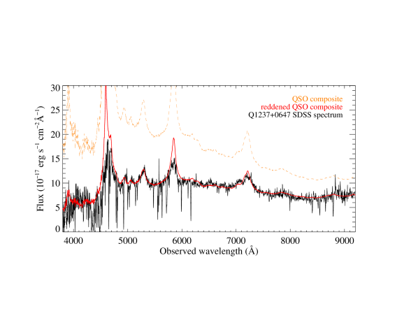
Figure 14: SDSS spectrum of J 1237$+$0647 (black). The orange dashed spectrum is the unreddened SDSS QSO composite spectrum (Vanden Berk et al., 2001). The red spectrum is the composite spectrum reddened by a SMC extinction law with E(B-V) = 0.053 (i.e. $A_{\rm V}$ = 0.14, in the rest-frame of the absorber). The fit was performed using an IDL code based on MPFIT (Markwardt, 2009).

4.3 The molecular fractions of H and C

In Fig. 15, we plot the ratios $N($CO)/$N($H₂) and $N($CO)/$N($C⁰) versus the hydrogen molecular fraction, $f_{\rm H2}$, for the two systems towards J 1237$+$0647 (this work) and J 1439+1117 (Srianand et al. 2008) together with measurements in the ISM of the Galaxy (Burgh et al., 2010). The latter authors define translucent clouds as clouds with CO)/H₂ $>$ 10^-6 and CO/C⁰ $>$ 1.0 for $f_{\rm H2}$ $>$ 0.4. In the cloud toward J 1237$+$0647, we find $N($CO)/$N($H₂) = 10^-5 for $\left<f_{\rm H2}\right>$ $=$ 0.24. However, as discussed previously, the hydrogen molecular fraction in the CO-bearing cloud is larger than this. In addition, the amount of carbon in CO molecules is about that in atomic form . We therefore conclude that the cloud in front of J 1237$+$0647 is indeed a translucent cloud, an ideal laboratory from probing astrochemistry at high redshift.

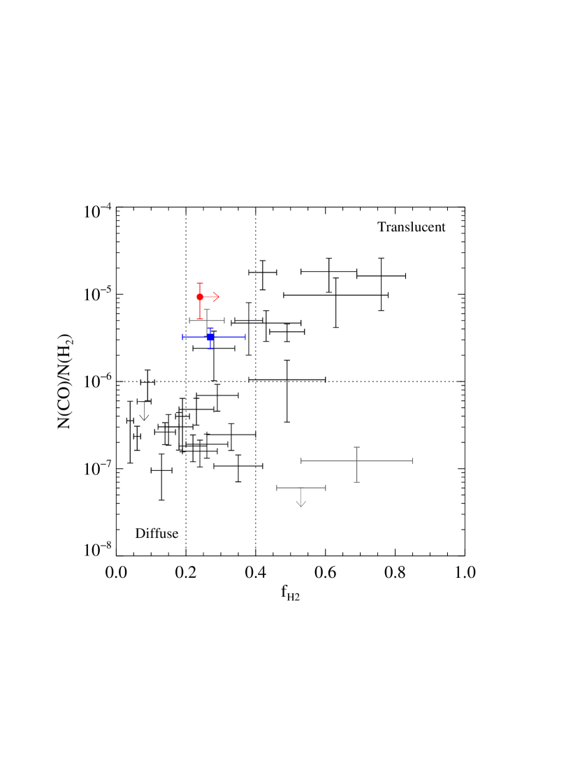
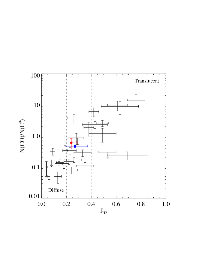
Figure 15: $N($CO)/$N($H₂) and $N($CO)/$N($C⁰) versus the molecular fraction, $f_{\rm H2}$. The red filled circle with error bars is our measurement at $z=2.7$ towards J 1237$+$0647 while the blue square represents the measurement at $z=2.4$ towards J 1439$+$1117 (Srianand et al., 2008b). Other points represent measurements in the Galactic ISM with three outliers represented in grey (Burgh et al., 2010). These are peculiar systems with uncertain measurements by the same authors. The horizontal dotted line marks the limit between diffuse and translucent clouds, while the two vertical dotted lines mark the transition range between these two regimes. Note that the molecular fraction we indicates toward J 1237$+$0647 is a lower limit. In order to enable easy comparison with local values, we use $N$(C${}^{0})$ measured with the $f$-values from Jenkins & Tripp (2001).

5 Conclusion

From our VLT survey for H₂ in DLAs, it appears that neutral carbon is generally observed in the same components that feature H₂ (Srianand et al., 2005; Noterdaeme et al., 2008a). We therefore selected the rare SDSS lines of sight in which C i absorptions are present. From UVES follow-up observations, we have detected strong absorptions from H₂, HD and CO along SDSS J123714.60$+$064759.5. This is a beautiful and peculiar case where detailed analysis of the physical properties of the gas is possible.

The H⁰ column density is small, $\log N$(H⁰) = 20.00$\pm$0.15 and corresponds to what is usually called a sub-DLA (Péroux et al., 2002). Corresponding overall metallicity is super solar with [Zn/H] = +0.34 and [S/H] =+0.15 . The system features three H₂ components spanning $\sim$125 km s^-1, the strongest of which, with $\log N$(H₂) = 19.20, does not coincide with the centre of the H i absorption. This means that the molecular fraction in this component is larger than the mean molecular fraction $\left<f_{\rm H2}\right>$ = 1/4 in the system.

From the populations of the low H₂ rotational levels, we measure the kinetic temperature of the gas to be around 100 K in the strongest component, where HD and CO are also detected. The detection of S⁰ and C⁰ implies that the gas is shielded from the surrounding far-UV radiation field.

The relative populations of the C⁰ fine structure levels yields an estimate of the average hydrogen density in the main component of about 50-60 cm^-3. At such densities, collisions are not frequent enough to dominate the rotational excitation of CO molecules and radiative processes are likely to determine the CO rotational populations. The excitation temperature we measure ($T_{\rm ex}$(CO)=10.5 K) is significantly larger than that measured in the local ISM ($T_{\rm ex}$(CO) $\sim 3.5$ K) for similar CO column densities, molecular fractions and kinetic temperatures. We show that the higher rotational excitation of CO towards J 1237$+$0647 results from the higher temperature of the Cosmic Microwave Background at the redshift of the absorber, $T_{\rm CMB}(z=2.69)$ = 10.05 K. This provides a strong positive test to the hot Big-Bang theory.

Small velocity shifts (of the order of 1 ${\rm km\,s^{-1}}$) are observed between the different neutral and molecular species in the main component. For H₂, the shift might appear more important but is rather due to the H₂ component being a blend of several sub-components. Neutral chlorine is likely a better indicator of the strongest molecular component (Sonnentrucker et al., 2006). Srianand et al. (2010) recently observed similar small velocity shifts between H₂ and 21-cm absorption in a high redshift DLA also testifying the presence of inhomogeneities of the ISM on very small scales. In turn, since the distribution of H⁰ and O⁰ are expected to closely follow each other, the O i$\lambda$1302 absorption profile indicates that atomic hydrogen is distributed over the full $\sim$400 km s^-1 velocity range over which metals are observed. This explains the large velocity shift between the centroid of H i and molecular lines.

All this reinforces the view that the ISM is patchy, with small and dense molecular cloudlets (probably with an onion-like structure) immersed in a warmer diffuse atomic medium (see e.g. Petitjean et al., 1992). We can derive an upper limit on the size of the molecular-rich region along the line-of-sight by considering that all H⁰ is associated with the main velocity component of density $n_{\rm H}$ = 50 cm^-3. The corresponding characteristic length is $l=N$(H${}^{0})/n_{\rm H^{0}}\simeq 0.6$ pc. A lower-limit can be put using Eq. A7 of Jura & York (1978, see also ) and the observed molecular and neutral chlorine fractions. This gives $l>0.05$ pc. The molecular region of the system has therefore a very small size and hence small cross-section. It is therefore not surprising that detections of translucent clouds were elusive till now. Studying the frequency of CO absorbers would give an idea of the filling factor of the molecular-rich gas, but requires larger statistics. Small physical extents could yield partial covering of the background source by the cloud. This may happen in particular if some absorption lines are redshifted on top of emission lines from the extended QSO broad line region, as seen in the case of Q 1232+082 (Ivanchik et al. 2010; Balashev et al., submitted).

Interestingly, the conclusion that the ISM at high redshift is made of small cold cloudlets immersed in warmer diffuse medium has been reached by Gupta et al. (2009) while considering the distribution of cold gas detected in 21-cm absorption. Note that J 1237$+$0647 is detected in the radio domain by FIRST. However, the low radio flux (2.3 mJy) prevents any spectroscopic study with current radio-telescopes.

Several chemical reactions can take place in this cloud. Indeed, three molecular species are detected, while the presence of neutral chlorine suggests chemical reactions involving HCl and HCl⁺ (e.g. Dalgarno et al., 1974; Neufeld & Wolfire, 2009). The DLA system toward J 1237$+$0647 is therefore an excellent candidate to target with future extremely large telescopes (ELTs) to detect other molecular species like C₂, CH, OH and study astrochemistry in the interstellar medium of high redshift galaxies. Given the expected attenuation of the quasar by CO-bearing clouds, X-shooter, with its high throughput and medium resolution, is the best instrument to survey carefully selected DLA/sub-DLA candidates for CO absorptions and build a sample of molecular-rich clouds at high redshift, which may then be studied in details in the optical and sub-millimeter ranges with future facilities like ELTs and ALMA.

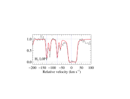
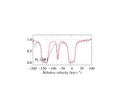
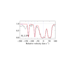
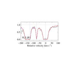
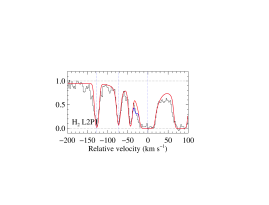
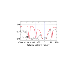
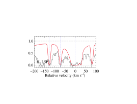
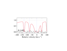
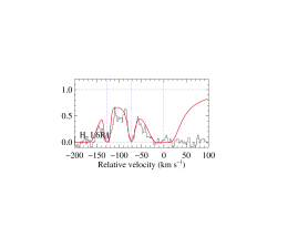
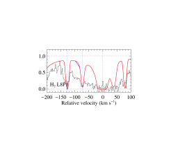
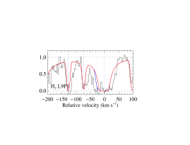
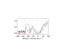
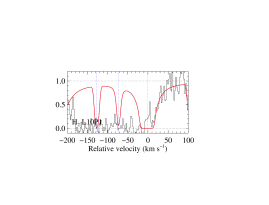
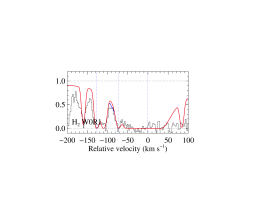
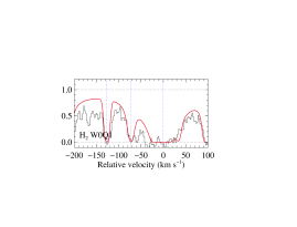
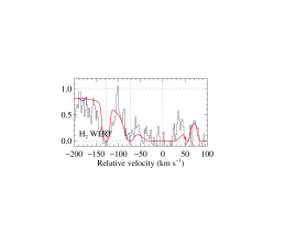
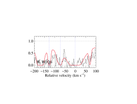
Figure 17: Fit to H₂(J=1) lines.

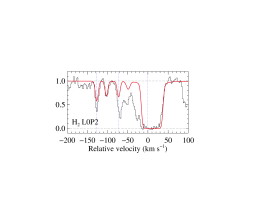
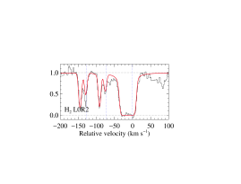
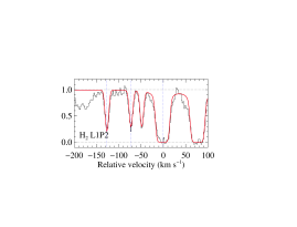
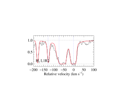
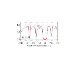
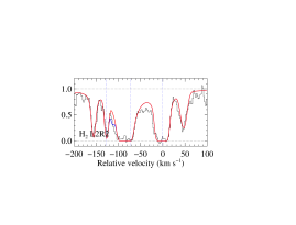
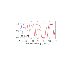
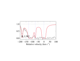
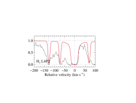
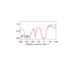
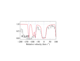
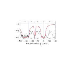
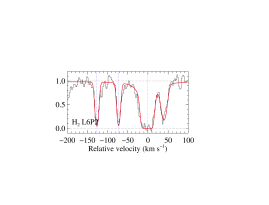
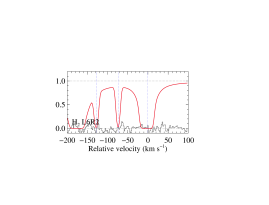
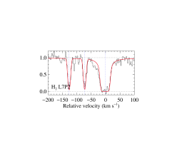
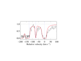
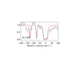
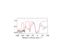
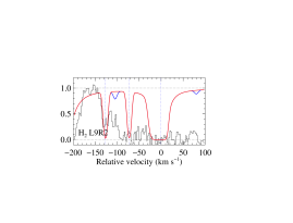
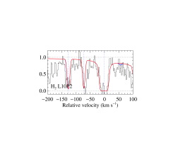
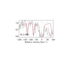
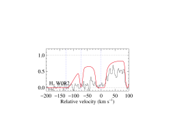
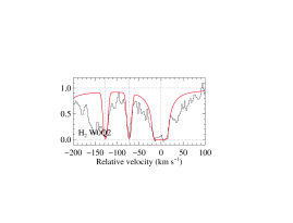
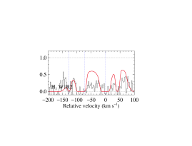
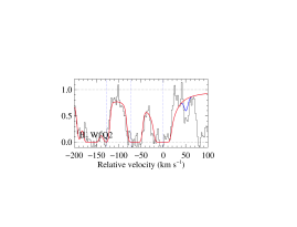
Figure 18: Fit to H₂(J=2) lines.

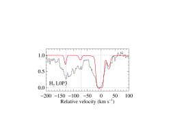
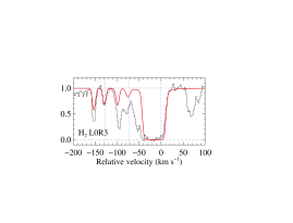
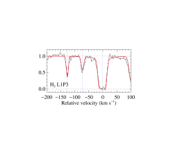
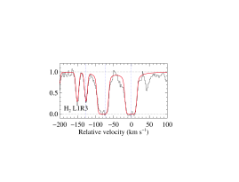
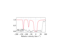
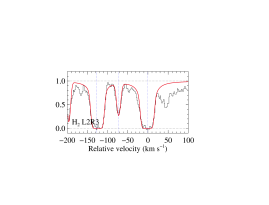
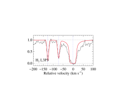
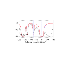
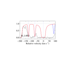
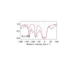
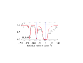
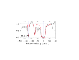
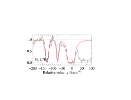
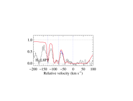
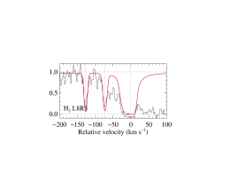
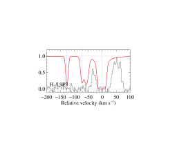
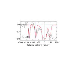
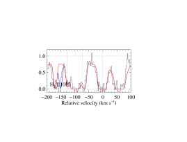
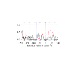
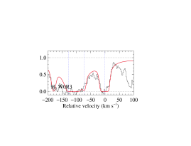
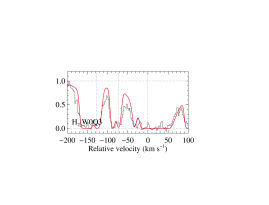
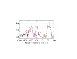
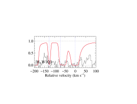
Figure 19: Fit to H₂(J=3) lines.

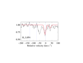
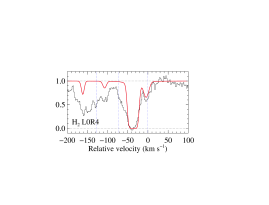
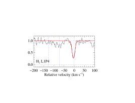
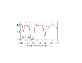
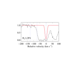
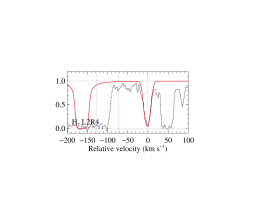
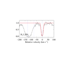
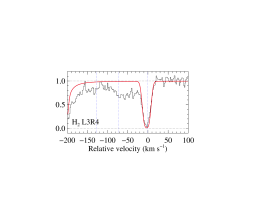
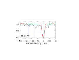
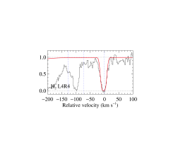
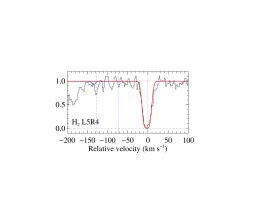
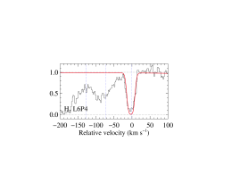
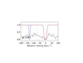
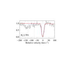
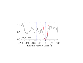
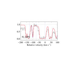
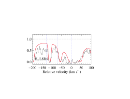
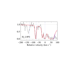
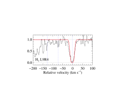
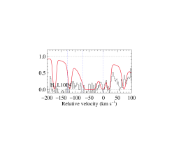
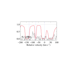
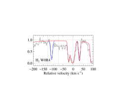
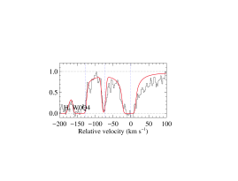
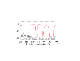
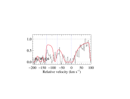
Figure 20: Fit to H₂(J=4) lines.

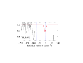
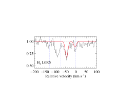
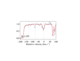
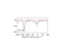
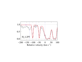
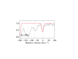
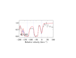
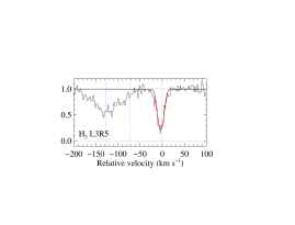
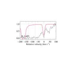
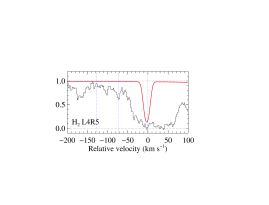
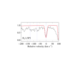
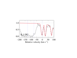
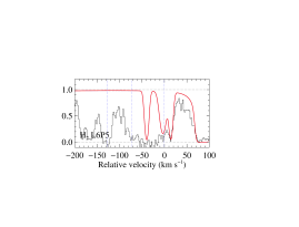
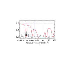
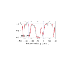
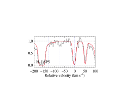
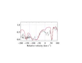
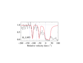
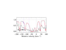
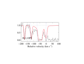
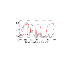
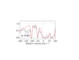
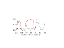
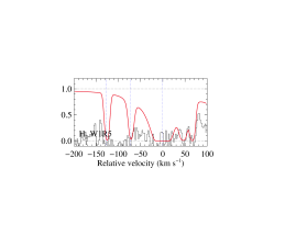
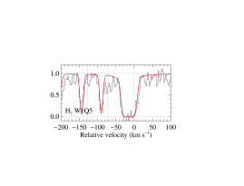
Figure 21: Fit to H₂(J=5) lines.