Halo Clustering with Non-Local Non-Gaussianity

Abstract

We show how the peak-background split can be generalized to predict the effect of non-local primordial non-Gaussianity on the clustering of halos. Our approach is applicable to arbitrary primordial bispectra. We show that the scale-dependence of halo clustering predicted in the peak-background split (PBS) agrees with that of the local-biasing model on large scales. On smaller scales, $k\gtrsim 0.01\,h~{}{\rm Mpc}^{-1}$, the predictions diverge, a consequence of the assumption of separation of scales in the peak-background split. Even on large scales, PBS and local biasing do not generally agree on the amplitude of the effect outside of the high-peak limit. The scale dependence of the biasing—the effect that provides strong constraints to the local-model bispectrum—is far weaker for the equilateral and self-ordering-scalar-field models of non-Gaussianity. The bias scale dependence for the orthogonal and folded models is weaker than in the local model ($\sim k^{-1}$), but likely still strong enough to be constraining. We show that departures from scale-invariance of the primordial power spectrum may lead to order-unity corrections, relative to predictions made assuming scale-invariance—to the non-Gaussian bias in some of these non-local models for non-Gaussianity. An Appendix shows that a non-local model can produce the local-model bispectrum, a mathematical curiosity we uncovered in the course of this investigation.

I Introduction

An active effort to seek departures from Gaussianity in primordial cosmological perturbations is currently under way Bernardeau:2001qr . The motivation stems from the desire to learn more about inflation inflation ; NGReview . The simplest single-field slow-roll (SFSR) inflation models predict that any departures from Gaussianity should be undetectably small localmodel . However, theorists generally consider these to be toy models, or effective theories, and there should be, at some point, phenomena that depart from the predictions of these simplest models. Many physics models for inflation larger ; curvaton ; Dvali:1998pa , or alternatives/additions to inflation topdefects ; Figueroa:2010zx , do in fact make predictions for non-Gaussianity at a much higher level than those of SFSR inflation.

It has been proposed to search for primordial non-Gaussianity through a variety of techniqes, including cluster, void, and high-redshift-galaxy abundances and properties abundances ; Verde:2000vq . Primordial non-Gaussianity had long been sought with large-scale-structure surveys LSS , but the sensitivity of these surveys had generally been weak compared with that due to the CMB Verde:1999ij ; limits ; Komatsu:2010fb . It has recently been shown, however, that the effects of primordial non-Gaussianity may be amplified in the clustering of dark-matter halos Dalal:2007cu ; Slosar:2008hx ; Matarrese:2008nc ; DesjacquesSeljak . The number density of halos is determined by the threshold overdensity for gravitational collapse. In a region with a long-wavelength overdensity, the upward fluctuation required for collapse is reduced and the abundance of objects thus higher. However, in non-Gaussian models, the local power spectrum (or density-fluctuation amplitude) may also be affected by the local long-wavelength overdensity. If so, this provides an additional dependence of the local abundance of halos on the long-wavelength density field. In the local-model of non-Gaussianity, this leads to a rapid increase in the biasing of halos on large scales. Null searches for this large-scale enhancement place constraints to primordial non-Gaussianity that are competitive with those from the CMB Slosar:2008hx ; Xia:2010yu .

Still, the local model is just one of many possible models for non-Gaussianity, and it is natural to inquire how other forms of non-Gaussianity, described by other bispectra, may affect biasing. This question was tackled in Ref. Verde:2009hy using local Lagrangian biasing (LLB) Matarrese:1986et to model the clustering of halos. However, different analytic descriptions of biasing that make similar predictions at lowest order may differ at higher order Catelan:2000vn , and so it is important to investigate different biasing models to understand better the model predictions and theoretical uncertainties. In this paper, we calculate the clustering of halos for a general primordial bispectrum using the peak-background split (PBS). Our approach generalizes that in Refs. Dalal:2007cu ; Slosar:2008hx (see also GiannantonioPorciani ) and complements the local-bias calculation of Ref. Verde:2009hy .

As examples, we apply our results to the equilateral Equil , folded folded , orthogonal Senatore:2009gt , and self-ordering-scalar-field (SOSF) Figueroa:2010zx bispectra, as well as the local-model bispectrum Luo:1993xx ; Verde:1999ij . We find that the scale-dependence of the biasing—the effect that leads to strong constraints to the local-model bispectrum where the bias correction goes as $k^{-2}$ —disappears for the equilateral and self-ordering-scalar-field models. While the scale dependence for the orthogonal and folded models is weaker than in the local model ($\sim k^{-1}$), it may still be strong enough to be constraining. We also find that small departures from scale-invariance in the primordial power spectrum may lead to large corrections to the non-Gaussian bias for some of these non-Gaussian models, especially for the equilateral and SOSF models.

We show that while the PBS prediction for the scale-dependence of halo clustering for general bispectra agrees with the LLB predictions at large scales, they differ at small scales, a breakdown of the separation of scales assumed in the PBS. Furthermore, the amplitude of the non-Gaussian halo bias is determined by different quantities in both approaches, and these quantities do not in general agree outside a specific high-peak limit of local biasing.

The paper is structured as follows: we review the case of general, quadratic primordial non-Gaussianity in § II. § III presents the peak-background split argument, and § IV derives the non-Gaussian halo bias in this approach. § V contains some results on the squeezed limit of different primordial bispectra. Finally, we compare the PBS and local-biasing approaches in § VI, and conclude in § VII. An Appendix shows that the local-model bispectrum can arise from a non-local model, a mathematical curiosity that arose during the development of the formalism in this paper.

II General quadratic non-Gaussianity

II.1 Basic formalism

Suppose the primordial potential $\Phi$ is a general, non-local quadratic function of a Gaussian field $\phi$. Expressed in real space, the most general expression preserving statistical homogeneity and isotropy is a two-dimensional convolution,

$$\Phi(\mathbf{x})=\phi(\mathbf{x})+f_{\rm NL}\int d^{3}y\int d^{3}z\;W(\mathbf{y},\mathbf{z})\phi(\mathbf{x}+\mathbf{y})\phi(\mathbf{x}+\mathbf{z}),$$ (1)

where the kernel $W(\mathbf{y},\mathbf{z})$ is only a function of $y$, $z$, and $\mathbf{\hat{y}}\cdot\mathbf{\hat{z}}$ and is symmetric, $W(\mathbf{y},\mathbf{z})=W(\mathbf{z},\mathbf{y})$. Here, the non-Gaussianity amplitude is quantified by the parameter $f_{\rm NL}$. Although the spatial average of $\Phi$ is not zero, but of order $\langle\phi^{2}\rangle$, this constant offset is unobservable and can be eliminated by a gauge transformation.

In Fourier space, Eq. (1) reads

$$\Phi(\mathbf{k})=\phi(\mathbf{k})+ f_{\rm NL}\int\frac{d^{3}k_{1}}{(2\pi)^{3}}$$ (2)

$$\times\widetilde{W}(\mathbf{k}_{1},\mathbf{k}-\mathbf{k}_{1})\phi(\mathbf{k}_{1})\phi(\mathbf{k}-\mathbf{k}_{1}),$$

where $\widetilde{W}$ is the Fourier transform,

$$\widetilde{W}(\mathbf{k}_{1},\mathbf{k}_{2})=\int d^{3}y\int d^{3}z\>e^{-i\mathbf{k}_{1}\cdot\mathbf{y}-i\mathbf{k}_{2}\cdot\mathbf{z}}W(\mathbf{y},\mathbf{z}).$$ (3)

Statistical homogeneity requires that $\widetilde{W}$ has no dependence on the directions of $\mathbf{k}_{1}$ and $\mathbf{k}_{2}$, only on their relative directions. It is thus a function only of the magnitudes $k_{1}$ and $k_{2}$ (and symmetric in these arguments) and the dot product $\mathbf{k}_{1}\cdot\mathbf{k}_{2}$. It can thus alternatively be written as a function $\widetilde{W}(k_{1},k_{2},k_{3})$ of the magnitude $k_{3}=|\mathbf{k}_{1}+\mathbf{k}_{2}|$ of the third side of the triangle constructed from $\mathbf{k}_{1}$ and $\mathbf{k}_{2}$.

The leading non-Gaussian correction to the potential is commonly parametrized in terms of the bispectrum $B(k_{1},k_{2},k_{3})$ of $\Phi$, defined by,

$$\langle\Phi(\mathbf{k}_{1})\Phi(\mathbf{k}_{2})\Phi(\mathbf{k}_{3})\rangle=\;(2\pi)^{3}\delta_{D}(\mathbf{k}_{1}+\mathbf{k}_{2}+\mathbf{k}_{3})B_{\Phi}(k_{1},k_{2},k_{3}),$$ (4)

where $\delta_{D}$ is a Dirac delta function. It is straightforward to calculate the bispectrum of $\Phi$ given Eq. (2). We obtain

$$B_{\Phi}(k_{1},k_{2},k_{3})=2f_{\rm NL}\bigg{\{} \widetilde{W}(\mathbf{k}_{1},\mathbf{k}_{2})P_{\Phi}(k_{1})P_{\Phi}(k_{2})$$ (5)

$$+2\>\mbox{perm.}\bigg{\}}.$$

Here, $P_{\Phi}(k)$ denotes the power spectrum of $\Phi$, which to leading order in $f_{\rm NL}$ agrees with that of $\phi$. The two permutations not written are the two remaining cyclic permutations of $k_{1},k_{2},k_{3}$. The requirement of statistical isotropy dictates that $B_{\Phi}$ is a function only of the triangle shape, not its orientation, and so the bispectrum can be written as a function $B_{\Phi}(k_{1},k_{2},k_{3})$ only of the magnitudes of its three arguments. The Fourier-space kernel $\widetilde{W}$ is, on the other hand, only required to be symmetric under exchange of its two (vectorial) arguments. Hence, Eq. (5) does not uniquely define $\widetilde{W}$; there may be several different $\widetilde{W}$ that yield the same bispectrum (note however that these will give different trispectra at order $f_{\rm NL}^{2}$).

The ambiguity in $\widetilde{W}$ can be eliminated if we assume, for example, that it is symmetric under exchange of its three arguments. With this additional assumption, the Fourier-space kernel can be written in terms of the bispectrum as

$$\widetilde{W}_{\mathrm{sym}}(k_{1},k_{2},k_{3})\equiv\frac{1}{2f_{\rm NL}}\frac{B_{\Phi}(k_{1},k_{2},k_{3})}{P_{1}P_{2}+P_{1}P_{3}+P_{2}P_{3}},$$ (6)

where $P_{i}\equiv P_{\Phi}(k_{i})$. Eq. (6) becomes more clear by considering concrete examples. In the local model, the bispectrum is given by localmodel ; Luo:1993xx ; Verde:1999ij

$$B^{\rm loc}_{\Phi}(k_{1},k_{2},k_{3})=2f_{\rm NL}\left[P_{\Phi}(k_{1})P_{\Phi}(k_{2})+2\;\mbox{perm.}\right].$$ (7)

Applying Eq. (6) immediately yields

$$\widetilde{W}^{\rm loc}_{\mathrm{sym}}(k_{1},k_{2},k_{3})=1,$$ (8)

and going back to real-space, we obtain

$$W^{\rm loc}(\mathbf{y},\mathbf{z})=\delta_{D}(\mathbf{y})\delta_{D}(\mathbf{z}).$$ (9)

This, together with Eq. (1), yields the well-known local expression for $\Phi$,

$$\Phi(\mathbf{x})=\phi(\mathbf{x})+f_{\rm NL}\phi^{2}(\mathbf{x}).$$ (10)

Finally, we note that the prediction of the scale-dependent non-Gaussian halo bias on large scales does not depend on the particular choice of kernel. As we will see in § IV, this prediction depends on the squeezed limit of the kernel, where $k_{2}\gg k_{1}$. Denoting $q=k_{1}/k_{2}$, this limit corresponds to $q\rightarrow 0$, and in the same limit Eq. (5) can be written as

$$\widetilde{W}(\mathbf{k}_{1},\mathbf{k}_{2})\stackrel{{\scriptstyle\rm squeezed}}{{=}}\frac{B_{\Phi}(k_{1},k_{2},k_{3})}{4f_{\rm NL}P_{\Phi}(k_{1})P_{\Phi}(k_{2})}\left(1+\mathcal{O}(q)\right).$$ (11)

Thus, in the squeezed limit the kernel $\widetilde{W}$ and in particular its leading scaling with $q$ are uniquely specified. Furthermore, Eq. (5) also shows that all kernels agree for equilateral triangles, further restricting the magnitude of the kernel-choice ambiguity. In § V we will return to the squeezed limit of $\widetilde{W}$ and show how it determines the scale-dependence of the non-Gaussian halo bias.

II.2 Some primordial bispectra

We now summarize other non-local bispectra that have been discussed in the recent literature and that we will consider here. All of these bispectra are scale-free [i.e. they scale as $P_{\Phi}^{2}$ under a uniform rescaling of all $k_{i}$], but we reiterate that this is not necessary for Eqs. (2) and (6) to apply. These bispectra simplify considerably in the squeezed limit, which we will discuss in § V.

In the equilateral model Equil , the bispectrum is given by

$$B_{\Phi}^{\rm eql}=6f_{\rm NL}\big{[} (-P_{1}P_{2}-2\>\mbox{perm.})-2(P_{1}P_{2}P_{3})^{2/3}$$

$$+(P_{1}^{1/3}P_{2}^{2/3}P_{3}+5\>\mbox{perm.})\big{]}.$$ (12)

The folded bispectrum is given by folded

$$B_{\Phi}^{\rm fol}=6f_{\rm NL}\big{[} (P_{1}P_{2}+2\>\mbox{perm.})+3(P_{1}P_{2}P_{3})^{2/3}$$

$$-(P_{1}^{1/3}P_{2}^{2/3}P_{3}+5\>\mbox{perm.})\big{]}.$$ (13)

The orthogonal bispectrum is given by Senatore:2009gt

$$B_{\Phi}^{\rm orth}=6f_{\rm NL}\Big{\{} -3\left(P_{1}P_{2}+2\,\mathrm{perms}\right)-8(P_{1}P_{2}P_{3})^{2/3}$$

$$+3\left[(P_{1}P_{2}^{1/3}P_{3}^{2/3})+5\,\mathrm{perms}\right]\Big{\}}.$$ (14)

The bispectrum due to self-ordering scalar fields (SOSFs) is Figueroa:2010zx

$$B_{\Phi}^{\rm SOSF} = 437\,f_{\rm NL}\left(P_{1}P_{2}P_{3}\right)^{2/3}\left(1-0.485\frac{k_{2}}{k_{1}}\right)$$ (15)

$$\times\frac{k_{3}}{k_{1}}\left[1-1.87\frac{k_{3}}{k_{1}}+0.945\left(\frac{k_{3}}{k_{1}}\right)^{2}\right],$$

where in this case we restrict $k_{1}\geq k_{2}\geq k_{3}$. We adopt the usual convention of defining $f_{\rm NL}$ so that $B_{\Phi}=6f_{\rm NL}(P_{\Phi})^{2}$ for equilateral triangles ($k_{1}=k_{2}=k_{3}$), except for the folded bispectrum, which is zero for equilateral triangles.

II.3 Relating the processed and primordial power spectra

So far we have been discussing the primordial potential and its power spectrum and bispectrum, but what we need for galaxy clustering is the processed potential. The processed potential, which we denote with a subscript “0,” is related to the primordial potential in Fourier space via $\Phi_{0}(\mathbf{k})=T(k)\Phi(\mathbf{k})$, where $T(k)$ is the transfer function. If we similarly define a processed Gaussian random field $\phi_{0}(\mathbf{k})=T(k)\phi(\mathbf{k})$, then the processed potential may be written,

$$\Phi_{0}(\mathbf{k})=\phi_{0}(\mathbf{k})+ f_{\rm NL}\int\frac{d^{3}k_{1}}{(2\pi)^{3}}$$ (16)

$$\times\widetilde{W}_{0}(\mathbf{k}_{1},\mathbf{k}-\mathbf{k}_{1})\phi_{0}(\mathbf{k}_{1})\phi_{0}(\mathbf{k}-\mathbf{k}_{1}),$$

in terms of a processed kernel,

$$\widetilde{W}_{0}(\mathbf{k}_{1},\mathbf{k}_{2})=\frac{T(|\mathbf{k}_{1}+\mathbf{k}_{2}|)\widetilde{W}(\mathbf{k}_{1},\mathbf{k}_{2})}{T(k_{1})T(k_{2})}.$$ (17)

Note that even if we choose $\widetilde{W}(\mathbf{k}_{1},\mathbf{k}_{2})$ to be a symmetric function $\widetilde{W}_{\mathrm{sym}}(k_{1},k_{2},k_{3})$ of the three magnitudes $k_{1}$, $k_{2}$, $k_{3}$, the processed kernel, $\widetilde{W}_{0}(k_{1},k_{2},k_{3})$ is not symmetric under exchange of all three arguments. Still, it is symmetric under exchange of its two vectorial arguments if written $\widetilde{W}_{0}(\mathbf{k}_{1},\mathbf{k}_{2})$. The configuration-space kernel $\widetilde{W}_{0}(\mathbf{y},\mathbf{z})$ is then obtained from the Fourier transform of $\widetilde{W}_{0}(\mathbf{k}_{1},\mathbf{k}_{2})$. It is this processed kernel that will appear in the analysis below.

Alternatively, one can define the processed kernel $\widetilde{W}_{0}$ directly from the bispectrum and power spectrum of the processed potential $\Phi_{0}$, in analogy with Eq. (6):

$$\widetilde{W}_{0}(\mathbf{k}_{1},\mathbf{k}_{2})=\frac{1}{2f_{\rm NL}}\frac{B_{\Phi_{0}}(k_{1},k_{2},|\mathbf{k}_{1}+\mathbf{k}_{2}|)}{P_{\Phi_{0}}(k_{1})P_{\Phi_{0}}(k_{2})+{\rm cyc.}},$$ (18)

where

$$B_{\Phi_{0}}(k_{1},k_{2},k_{3})=\> T(k_{1})T(k_{2})T(k_{3})B_{\Phi}(k_{1},k_{2},k_{3}),$$ (19)

$$P_{\Phi_{0}}(k)=\> T^{2}(k)P_{\Phi}(k).$$ (20)

Note, however, that if we choose the processed kernel to be symmetric in all three arguments, then the primordial kernel will no longer be symmetric. That is, either the primordial or the processed kernel may be fully symmetric, but not both.

In our analysis below, we will consider these two forms for $\widetilde{W}_{0}$, one (which we label with the subscript “1”) in which the primordial kernel is fully symmetric, and one (which we label with the subscript “2”) in which the processed kernel is symmetric. To be clear, the two kernels we consider below are

$$\widetilde{W}_{01}(\mathbf{k}_{1},\mathbf{k}_{2})\equiv\frac{T(|\mathbf{k}_{1}+\mathbf{k}_{2}|)}{T(k_{1})T(k_{2})}\widetilde{W}_{\mathrm{sym}}(\mathbf{k}_{1},\mathbf{k}_{2}),$$ (21)

and

$$\widetilde{W}_{02}(\mathbf{k}_{1},\mathbf{k}_{2})\equiv\frac{1}{2f_{\rm NL}}\frac{B_{\Phi_{0}}(k_{1},k_{2},|\mathbf{k}_{1}+\mathbf{k}_{2}|)}{P_{\Phi_{0}}(k_{1})P_{\Phi_{0}}(k_{2})+{\rm cyc.}}.$$ (22)

There are, of course, other kernels one could choose. However, with any definition, $\widetilde{W}_{0}=\widetilde{W}$ whenever all three $\mathbf{k}$ vectors are sufficiently small so that $T(k)\simeq 1$. Moreover, they have the same squeezed limits:

$$\widetilde{W}_{0}(\mathbf{k}_{1},\mathbf{k}_{2})\stackrel{{\scriptstyle k_{2}\gg k_{1}}}{{\longrightarrow}} \frac{1}{T(k_{1})}\widetilde{W}(\mathbf{k}_{1},\mathbf{k}_{2})$$ (23)

$$=\> \frac{1}{T(k_{1})}\frac{B_{\Phi}(k_{1},k_{2},k_{3})}{2f_{\rm NL}P_{\Phi}(k_{1})P_{\Phi}(k_{2})},$$

where we have used Eq. (11) for the last equality. This shows that the processed kernel is uniquely specified in the squeezed limit as well. Further, $\widetilde{W}_{01}$ and $\widetilde{W}_{02}$ also have the same equilateral limits, which further restricts the numerical uncertainty associated with this theoretical ambiguity. Finally, note that $\widetilde{W}_{0}\neq 1$ in general for the local model, even though $\widetilde{W}$ is unity. This reflects the fact that the relation between the primordial and processed potentials (and matter perturbations) is non-local.

Before proceeding, we note that one consequence of our approach is the realization that a non-local inflationary model can give rise to the local-model primordial bispectrum. This is spelled out in the Appendix.

III Peak-background split for general quadratic non-Gaussianity

The physical, non-Gaussian, matter-density perturbation $\hat{\delta}$ is related to the processed potential $\Phi_{0}$ through the Poisson equation,

$$\frac{\nabla^{2}}{a^{2}}\Phi_{0}=4\pi G\>\bar{\rho}\>\hat{\delta}.$$ (24)

Similarly, we can define a fictitious Gaussian density field $\delta$ related to the Gaussian potential $\phi_{0}$ by the same relation. In Fourier space, these relations read,

$$\hat{\delta}(\mathbf{k},z) = \frac{2}{3}\frac{k^{2}}{(1+z)\,H_{0}^{2}\Omega_{m}}g_{*}(z)\Phi_{0}(\mathbf{k},z_{*})$$ (25)

$$\equiv \mathcal{M}(k,z)\Phi_{0}(\mathbf{k},z_{*}),$$

$$\delta(\mathbf{k},z) = \mathcal{M}(k,z)\phi_{0}(\mathbf{k},z_{*}),$$ (26)

where $g_{*}(z)\propto(1+z)D(z)$ is the potential growth factor normalized to unity at last scattering (at which in our convention $f_{\rm NL}$ is defined).

In the peak-background split, we first divide any perturbation $A(\mathbf{x})$ into a short- and long-wavelength piece:

$$A(\mathbf{x})=A_{s}(\mathbf{x})+A_{l}(\mathbf{x}).$$ (27)

Here, the “long” wavelengths are those comparable to the distances over which we measure correlations. The “short” wavelengths are on much smaller scales, of order the Lagrangian extent of halos and less, whose peaks determine the locations of halos. For the Gaussian potential $\phi_{0}$, the two pieces $\phi_{l}\equiv\phi_{0,l}$ and $\phi_{s}\equiv\phi_{0,s}$ are uncorrelated. The non-Gaussianity of Eq. (2) however induces a coupling of long- and short-wavelength perturbations in the potential as well as the matter density. Using Eq. (1) and the Poisson equation, Eq. (24), we can write the density $\hat{\delta}$ in terms of the Gaussian long- and short-wavelength pieces,

$$\hat{\delta}(\mathbf{x}) = \delta_{l}(\mathbf{x})+\delta_{s}(\mathbf{x})+2f_{\rm NL}\int d^{3}x\int d^{3}y\;W_{0}(\mathbf{y},\mathbf{z})$$ (28)

$$\times\bigg{\{}\phi_{l}(\mathbf{x}+\mathbf{y})\left[\delta_{l}(\mathbf{x}+\mathbf{z})+\delta_{s}(\mathbf{x}+\mathbf{z})\right]$$

$$\quad\ +\phi_{s}(\mathbf{x}+\mathbf{y})\left[\delta_{l}(\mathbf{x}+\mathbf{z})+\delta_{s}(\mathbf{x}+\mathbf{z})\right]$$

$$\quad\ -\frac{1}{2}\bm{\nabla}_{x}\phi_{0}(\mathbf{x}+\mathbf{y})\cdot\bm{\nabla}_{x}\phi_{0}(\mathbf{x}+\mathbf{z})\bigg{\}}.$$

We are interested in the density field at the positions of density peaks. In those locations, we expect terms of the form $\phi_{0}\>\delta$ to be much larger than $(\bm{\nabla}\phi_{0})^{2}$, since $\delta$ is at least order unity, and additionally $\bm{\nabla}\phi_{0}$ is suppressed if we associate peaks in the density field with peaks in the potential (where $\bm{\nabla}\phi_{0}=0$).

Next, we are mainly interested in the non-Gaussian effects on small-scale modes $\hat{\delta}_{s}$, since those result in the leading effect on halo formation. Separating the purely long-wavelength parts, we have

$$\hat{\delta}_{s}(\mathbf{x}) = \delta_{s}(\mathbf{x})+2f_{\rm NL}\int d^{3}x\int d^{3}y\;W_{0}(\mathbf{y},\mathbf{z})$$

$$\times\bigg{\{}\phi_{l}(\mathbf{x}+\mathbf{y})\delta_{s}(\mathbf{x}+\mathbf{z})$$

$$\quad\ +\phi_{s}(\mathbf{x}+\mathbf{y})\left[\delta_{l}(\mathbf{x}+\mathbf{z})+\delta_{s}(\mathbf{x}+\mathbf{z})\right]\bigg{\}}.$$

We will now neglect the terms in the last line: $\phi_{s}\delta_{l}$ is very small, since $\phi_{s}\sim\phi_{l}$, and $\delta_{l}\ll\delta_{s}$; and $\phi_{s}\delta_{s}$, while large, adds a purely stochastic contribution on large scales. We then obtain the final expression for the effect of primordial non-Gaussianity on small-scale modes in the context of the peak-background split:

$$\hat{\delta}_{s}(\mathbf{x})=\; \delta_{s}(\mathbf{x})$$ (30)

$$+2f_{\rm NL} \int d^{3}x\int d^{3}y\;W_{0}(\mathbf{y},\mathbf{z})\phi_{l}(\mathbf{x}+\mathbf{y})\delta_{s}(\mathbf{x}+\mathbf{z}).$$

Equivalently, in Fourier space:

$$\hat{\delta}_{s}(\mathbf{k}_{s})=\; \delta_{s}(\mathbf{k}_{s})$$ (31)

$$+2f_{\rm NL} \int\frac{d^{3}k}{(2\pi)^{3}}\widetilde{W}_{0}(\mathbf{k},\mathbf{k}_{s}-\mathbf{k})\phi_{l}(\mathbf{k})\delta_{s}(\mathbf{k}_{s}-\mathbf{k}).$$

Note that by assumption, $k_{s}\gg k$: the effect on the small-scale modes is determined by the behavior of the bispectrum in the squeezed limit [Eq. (6)]. In the following, we denote short-wavelength modes with $k_{s}$, while $k$ will stand for long-wavelength modes. We reiterate that even for the local model, the coupling between density and potential is non-local, since $\widetilde{W}_{0}\neq 1$.

IV First-order, non-local halo bias

We assume that the number density of halos, per unit logarithmic mass, smoothed over a region of size $\lambda\gtrsim k_{s}^{-1}$ centered at position $\mathbf{x}$ is a function,

$$n=n\Bigl{(}M,z;\overline{\rho}\left[1+\delta_{l}(\mathbf{x})\right],P\bigl{(}k_{s},\delta_{l}(\mathbf{x})\bigr{)}\Bigr{)},$$ (32)

where $M$ is the halo mass, $z$ the redshift, $\bar{\rho}\>[1+\delta_{l}(\mathbf{x})]$ is the density of matter in that region, and $P(k_{s},\delta_{l}(\mathbf{x}))$ is the small-wavelength (linear) matter power spectrum in that region. In a smooth Universe—i.e., one with no long-wavelength fluctuations, $\delta_{l}=0$, the halo abundance is the same everywhere. But if $\delta_{l}\neq 0$, then there will be fluctuations in the halo abundance with long-range correlations determined by long-range correlations in the matter density. Note that if primordial perturbations are Gaussian, then $P(k_{s})$ is the same everywhere. If, however, primordial perturbations are non-Gaussian, and if that non-Gaussianity couples short- and long-wavelength modes of the density field, then the small-scale power spectrum $P(k_{s},\delta_{l}(\mathbf{x}))$ may vary from one point in the Universe to another, as written in Eq. (32).

Biasing describes the relative clustering of halos and matter. The Lagrangian bias $b_{L}$ is defined to be the ratio of the fractional halo- and matter-density perturbations. More precisely, here we will consider the scale-dependent bias $b_{L}(k)$ which describes the relative amplitudes of Fourier modes of the halo abundance and matter density. To proceed, consider a single Fourier mode $\delta_{l}(\mathbf{x})=\tilde{\delta}_{l}(k)e^{i\mathbf{k}\cdot\mathbf{x}}$ of the density field with wavevector $\mathbf{k}$ and amplitude $\tilde{\delta}_{l}(\mathbf{k})$. This Fourier mode induces a variation $\delta n(\mathbf{x})=\delta\tilde{n}(\mathbf{k})e^{i\mathbf{k}\cdot\mathbf{x}}$ with amplitude $\delta\tilde{n}(\mathbf{k})=(dn/d\tilde{\delta}(\mathbf{k}))_{\mathbf{x}=0,\delta_{l}=0}\;\tilde{\delta}_{l}(\mathbf{k})$. The scale-dependent Lagrangian bias is thus,

$$b_{L}(M,z;k) \equiv \frac{\delta\tilde{n}(\mathbf{k})/\bar{n}}{\delta\tilde{\rho}/\bar{\rho}}=\frac{d\ln\tilde{n}(\mathbf{k})}{d\tilde{\delta}_{l}(\mathbf{k})}$$

$$= \frac{\partial\ln\tilde{n}(\mathbf{k})}{\partial\delta_{l}(\mathbf{k})}+\sum_{\mathbf{k}_{s}}\frac{\partial\ln\tilde{n}(\mathbf{k})}{\partial P(k_{s})}\frac{\partial P(k_{s})}{\partial\tilde{\delta}_{l}(\mathbf{k})}.$$

Here, the wavenumbers $k$ of interest are for long-wavelength modes, those over which halo clustering is measured, and we have used the chain rule in the last line.

The first term in the last line of Eq. (IV) is the standard result, that obtained assuming Gaussian initial conditions. It evaluates to

$$b_{L}^{\mathrm{G}}(M,z)=\frac{1}{\bar{n}}\frac{\partial n(M,z;\overline{\rho},P)}{\partial\ln\overline{\rho}}-1.$$ (34)

The second term in the last line of Eq. (IV) arises if there are non-Gaussian initial conditions that correlate long- and short-wavelength modes. In this case, a change in $\tilde{\delta}_{l}(\mathbf{k})$ induces changes in $P(k_{s})$ for each $\mathbf{k}_{s}$ (hence the sum in Eq. (IV)) which then induce changes in $\tilde{n}(\mathbf{k})$.

To evaluate the partial derivatives $\partial P(k_{s})/\partial\tilde{\delta}_{l}(\mathbf{k})$, we multiply Eq. (30) by $\delta_{s}(\mathbf{x}^{\prime})$, letting $\mathbf{r}=\mathbf{x}-\mathbf{x}^{\prime}$, and take the expectation value. The first term that arises is the usual Gaussian two-point correlation function $\xi_{s}(r)$. The non-Gaussian correction—that which correlates short- and long-wavelength modes—is then

$$\Delta\xi_{s}(r) = 4f_{\rm NL}\int d^{3}y\int d^{3}z\;W_{0}(\mathbf{y},\mathbf{z})\phi_{l}(\mathbf{y})\xi_{s}(\mathbf{r}+\mathbf{z}),\quad\quad$$ (35)

where we have set $\mathbf{x}=0$ without loss of generality. We now use

$$\Delta\xi_{s}(r) = \int\frac{d^{3}k_{s}}{(2\pi)^{3}}e^{i\mathbf{k}_{s}\mathbf{r}}\Delta P(k_{s}).$$ (36)

Expressing all quantities by their Fourier transforms, and performing the $\mathbf{y},\mathbf{z}$ integrals yields,

$$\Delta\xi_{s}(r)=\; 4f_{\rm NL}\int\frac{d^{3}k_{s}}{(2\pi)^{3}}e^{i\mathbf{k}_{s}\mathbf{r}}\int\frac{d^{3}k_{1}}{(2\pi)^{3}}$$

$$\times\widetilde{W}_{0}(\mathbf{k}_{1},\mathbf{k}_{s}-\mathbf{k}_{1})\phi_{l}(\mathbf{k}_{1})P(k_{s}).$$ (37)

Hence, via Eq. (36), the effect of any quadratic primordial non-Gaussianity on the statistics of the short-wavelength modes is given by

$$\Delta P(k_{s})=4f_{\rm NL}\int\frac{d^{3}k_{1}}{(2\pi)^{3}}\widetilde{W}_{0}(\mathbf{k}_{1},\mathbf{k}_{s}-\mathbf{k}_{1})\phi_{l}(\mathbf{k}_{1})P(k_{s}).$$ (38)

From this, we obtain the required partial derivatives,

$$\frac{\partial P(k_{s})}{\partial\tilde{\delta}(\mathbf{k})}=\> \mathcal{M}^{-1}(k)\frac{\partial\Delta P(k_{s})}{\partial\phi_{l}(\mathbf{k})},$$ (39)

$$\frac{\partial\Delta P(k_{s})}{\partial\phi_{l}(\mathbf{k})}=\> 4f_{\rm NL}P(k_{s})\widetilde{W}(\mathbf{k},\mathbf{k}_{s}-\mathbf{k}),$$

recalling that $\phi_{l}$ refers to the processed potential. Replacing the sum $\sum_{\mathbf{k}_{s}}$ by an integral $\int d^{3}k_{s}/(2\pi)^{3}$, we then obtain for the second term in the last line of Eq. (IV) the non-Gaussian correction to the Lagrangian bias,

$$\Delta b_{L}(M,z;k) = 2f_{\rm NL}\mathcal{M}^{-1}(k)$$

$$\times \int\frac{d^{3}k_{s}}{(2\pi)^{3}}2\frac{\partial\ln n}{\partial P(k_{s})}\widetilde{W}_{0}(\mathbf{k},\mathbf{k}_{s}-\mathbf{k})P(k_{s}).$$

Thus, in general, non-Gaussianity changes the shape of $P(k_{s})$ as well as the amplitude. However, Eq. (LABEL:eq:Db-1) simplifies for a very broad class of mass-function models, which only depend on the power spectrum through an overall normalization. We will turn to this case next.

IV.1 Universal mass functions

Most of the commonly used parametrizations of the halo abundance $n(M,z;\overline{\rho},P)$ are so-called universal mass functions universal ; Verde:2000vq . They can be written as

$$n=\frac{\overline{\rho}}{M}\nu f(\nu)\frac{d\ln\nu}{d\ln M},$$ (41)

and thus only depend on cosmology through the background density of matter $\overline{\rho}$ and the quantity,

$$\nu=\frac{\delta_{c}^{2}}{\sigma^{2}_{R}(z)},$$ (42)

where $\delta_{c}\approx 1.686$ is the linearly extrapolated collapse threshold. Here, $\sigma_{R}^{2}$ is the variance of the density field on a scale $R$ related to $M$ by $M=4\pi/3\overline{\rho}R^{3}$,

$$\sigma_{R}^{2}=\int\frac{d^{3}k}{(2\pi)^{3}}F_{R}^{2}(k)P(k),$$ (43)

where $F_{R}$ is the Fourier transform of a real-space tophat filter. The parametrization, Eq. (41), is sufficient to obtain the Gaussian and non-Gaussian halo bias.

First, for the Gaussian halo bias we use Eq. (34). The effect of a long-wavelength perturbation $\delta_{l}$ on the collapse threhold is $\delta_{c}\rightarrow\delta_{c}-\delta_{l}$, as derived in Refs. Mo:1995cs ; Sheth:1999mn . This gives (see also Ref. Slosar:2008hx ),

$$b_{L}=\frac{\partial\ln n(\overline{\rho},\nu)}{\partial\delta_{l}}=-\frac{2\nu}{\delta_{c}}\frac{d\ln(\nu f(\nu))}{d\nu}.$$ (44)

On the other hand, it is clear from Eqs. (LABEL:eq:Db-1) and (41) that the non-Gaussian halo bias will only enter through

$$\frac{\partial\ln n(\overline{\rho},\nu)}{\partial\ln\sigma_{R}}=-2\nu\frac{d\ln(\nu f(\nu))}{d\nu}=b_{L}\delta_{c}.$$ (45)

Next, we again use the chain rule, and, from Eq. (43),

$$\frac{\partial\sigma_{R}^{2}}{\partial P(k_{s})}=F_{R}^{2}(k_{s}).$$ (46)

We then have

$$\Delta b_{L}(k)=\; 2f_{\rm NL}\mathcal{M}^{-1}(k)\frac{\partial\ln n}{\partial\ln\sigma_{R}}\frac{\sigma_{W}^{2}(k)}{\sigma_{R}^{2}},$$ (47)

$$\sigma_{W}^{2}(k)\equiv\; \int\frac{d^{3}k_{s}}{(2\pi)^{3}}P(k_{s})F_{R}^{2}(k_{s})\widetilde{W}_{0}(\mathbf{k},\mathbf{k}_{s}-\mathbf{k}).$$

The prefactor $\mathcal{M}^{-1}$ scales as $k^{-2}$. However, in general $\sigma_{W}^{2}$, which involves $\widetilde{W}_{0}(\mathbf{k}_{s},\mathbf{k})$, will depend on $k$ as well.

Making use of the bias relations derived above, we have

$$\Delta b_{L}(k)=2f_{\rm NL}\mathcal{M}^{-1}(k)b_{L}\delta_{c}\frac{\sigma_{W}^{2}(k)}{\sigma_{R}^{2}},$$ (48)

where, to clarify, the matter power spectrum $P(k)$ is related to the processed-potential power spectrum $P_{\Phi_{0}}(k)$ through $P(k)=[\mathcal{M}(k)]^{2}P_{\Phi_{0}}(k)$.

Let us first look at the local case. We use the squeezed limit [Eq. (23)] and $\widetilde{W}^{\rm loc}=1$. In this case, the change in the small-scale power spectrum is independent of $k_{s}$, so that only the overall amplitude is affected. We obtain:

$$\Delta b^{\rm local}_{L}(k)=2f_{\rm NL}\frac{1}{\mathcal{M}(k)T(k)}b_{L}\delta_{c},$$ (49)

exactly matching the results of Refs. Slosar:2008hx . We will quantify the regime of validity of the squeezed limit in § VI.

For a given bispectrum, Eq. (48) can be evaluated exactly in a straightforward way. However, it is also interesting to look at the scaling of the bispectrum in the squeezed limit, which allows for a simpler estimate of $\Delta b$.

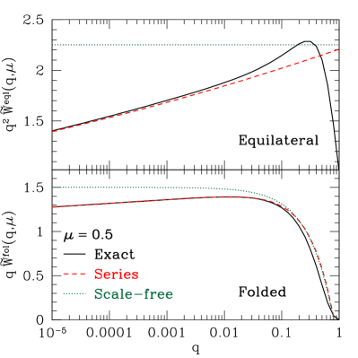
Figure 1: Squeezed limit of $\widetilde{W}(q,\mu)$ as function of $q$ for equilateral (top) and folded (bottom) bispectra. Here, we have taken out the leading $q$ scaling and adopted a fixed value of $\mu=0.5$. Shown is the exact result from Eq. (6), and the series expansion of the squeezed limit to $\mathcal{O}(q^{2},\varepsilon^{2})$ from § V. We also show the scale-free limit of this series expansion, which in general is not a good approximation.

V Squeezed limit and Scale-Dependence of Bias

As we have seen, the effect of primordial non-Gaussianity on the halo bias depends on $\widetilde{W}_{0}(\mathbf{k},\mathbf{k}_{s}-\mathbf{k})$, where $k_{s}\gg k$. This is known as the squeezed limit, since it corresponds to triangles where two sides are much longer than the third. In this Section, we derive the primordial kernel $\widetilde{W}(\mathbf{k},\mathbf{k}_{s}-\mathbf{k})$ in the squeezed limit to show analytically how the non-Gaussian bias will behave for the various bispectra we consider. To leading order, the processed kernel is then given by Eq. (23). For our numerical results in the next section, we will use the full kernels, Eqs. (21)–(22). For definiteness, we assume a flat $\Lambda$CDM cosmology throughout, with $n_{s}=0.958$, $\Omega_{m}=0.28$, $h=0.72$, and $\sigma_{8}=0.8$.

Let us define $q=k/k_{s}$ and $\mu=\mathbf{\hat{k}}\cdot\mathbf{\hat{k}}_{s}$. We then write the kernel as a power series in $q$. For example, in the simplest case, the local model, the squeezed limit is just $\widetilde{W}=1$. For the other bispectra, we use the $k$ scaling of $P_{\Phi}$,

$$P_{\Phi}(k)\propto k^{n_{s}-4}\equiv k^{-3+\varepsilon},\ \varepsilon=n_{s}-1,$$ (50)

where $\varepsilon\approx-0.04$ is the deviation from scale-free initial perturbations. The squeezed limit of the non-local bispectrum shapes introduced in § II can be easily derived in the limit of scale-free initial conditions. However, we will see that it is important to take into account a non-zero $n_{s}-1$. Since the prefactor in Eq. (LABEL:eq:Db-1) goes as $k^{-2}\propto q^{-2}$, we will expand $\widetilde{W}$ up to terms $\propto q^{2}$. We will also expand to second order in $\varepsilon$.

For the equilateral model, this gives,

$$\widetilde{W}^{\rm eql}(q,\mu) \stackrel{{\scriptstyle\rm squeezed}}{{=}}3q^{2}\>\bigg{(}1-\mu^{2}-\frac{2\varepsilon}{3}(\ln q-2\mu^{2})$$

$$\qquad\qquad\qquad+\frac{\varepsilon^{2}}{9}(2\ln^{2}q-\mu^{2})\bigg{)}$$ (51)

$$\stackrel{{\scriptstyle\rm scale-free}}{{=}}3q^{2}\>(1-\mu^{2}).$$ (52)

Thus, in the scale-free case, $\widetilde{W}^{\rm eql}$ scales exactly as $k^{2}/k_{s}^{2}$ in the squeezed limit, canceling the $k^{-2}$ prefactor in Eq. (LABEL:eq:Db-1) and leading to a scale-independent correction to the bias. This is not quite true in reality, since Eq. (51) contains logarithmic corrections, which can be quite important for $q\ll 1$ (Fig. 1). Note also that $\widetilde{W}=0$ for $\mu=1$ in the scale-free case, but is only suppressed by $2\varepsilon(\ln q-2)/3\approx-0.18$ for $q=0.01$.

For the folded model, we have,

$$\widetilde{W}^{\rm fol}(q,\mu)\stackrel{{\scriptstyle\rm squeezed}}{{=}}\frac{3}{2}q\Bigg{(}1+\left(4\mu^{2}+\mu-4\right)\frac{q}{2}$$

$$-\frac{\varepsilon}{3}\big{(}\ln q+\frac{q}{2}\>[8\mu^{2}+\mu+(\mu-8)\ln q]\big{)}$$ (53)

$$+\frac{\varepsilon^{2}}{18}\bigg{(}\ln^{2}q+\frac{q}{2}\>\big{[}8\mu^{2}+2\mu\ln q+(\mu-16)\ln^{2}q\big{]}\bigg{)}\Bigg{)}$$

$$\stackrel{{\scriptstyle\rm scale-free}}{{=}}\frac{3}{2}q+\frac{3}{4}q^{2}\>(4\mu^{2}+\mu-4).$$ (54)

In the scale-free case, the folded model shows a scaling proportional to $q$, with corrections going as $q^{2}$. Fig. 1 shows that the scale-free case matches the true squeezed limit somewhat more accurately than in the equilateral case.

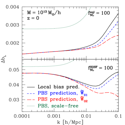
Figure 2: Non-Gaussian correction to the halo bias $\Delta b_{L}$ calculated in the peak-background-split (PBS) and local-bias approaches as a function of $k$, for the equilateral (top) and SOSF (bottom) bispectra. We have assumed $f_{\rm NL}=100$ in both cases and $M=10^{13}\,M_{\odot}/h$ halos at $z=0$. We also show the scale-free approximations Eqs. (58)–(60).

The squeezed limit for the orthogonal model is

$$\widetilde{W}^{\rm orth}(q,\mu)\stackrel{{\scriptstyle\rm squeezed}}{{=}}-3q\Bigg{(}1+\frac{q}{2}\left(6\mu^{2}+\mu-6\right)$$

$$+\frac{\varepsilon}{3}\big{(}-\ln q+\frac{q}{2}\>[-12\mu^{2}-\mu+(12-\mu)\ln q]\big{)}$$ (55)

$$+\frac{\varepsilon^{2}}{18}\bigg{(}\ln^{2}q+\frac{q}{2}\>\big{[}12\mu^{2}+2\mu\ln q+(\mu-24)\ln^{2}q\big{]}\bigg{)}\Bigg{)}$$

$$\stackrel{{\scriptstyle\rm scale-free}}{{=}}-3q+9q^{2}-\frac{3}{2}q^{2}(\mu+6\mu^{2}).$$ (56)

This bispectrum will therefore give rise to a scale-dependent bias similar to that for the folded model, but roughly twice as large in magnitude and opposite in sign.

For the SOSF model, the kernel reduces in the squeezed limit to

$$\widetilde{W}^{\rm SOSF}(q,\mu)\stackrel{{\scriptstyle\rm squeezed}}{{=}}56.26\>q^{2}\left(1-\frac{\varepsilon}{3}\ln q\left[1-\frac{\varepsilon}{6}\ln q\right]\right).$$ (57)

The $q^{2}$ scaling implies that this model will behave similarly to the equilateral model, although the prefactor of 56 indicates that the amplitude of the effect will be much larger for a given $f_{\rm NL}$.

As a rough approximation to the exact result for the non-Gaussian $\Delta b$, we can take the scale-free squeezed limit derived above and in addition ignore any $\mu$-dependence. From Eq. (23) and Eq. (48), we then obtain

$$\Delta b^{\rm eql}_{L}(k)\approx\; \frac{6f_{\rm NL}}{\mathcal{M}(k)T(k)}b_{L}\delta_{c}\;k^{2}\frac{\sigma_{R,-2}^{2}}{\sigma_{R}^{2}},$$ (58)

$$\Delta b^{\rm SOSF}_{L}(k)\approx\; \frac{112f_{\rm NL}}{\mathcal{M}(k)T(k)}b_{L}\delta_{c}\;k^{2}\frac{\sigma_{R,-2}^{2}}{\sigma_{R}^{2}},$$ (59)

$$\Delta b^{\rm fol}_{L}(k)\approx\; \frac{3f_{\rm NL}}{\mathcal{M}(k)T(k)}b_{L}\delta_{c}\;k\frac{\sigma_{R,-1}^{2}}{\sigma_{R}^{2}},$$ (60)

$$\Delta b^{\rm orth}_{L}(k)\approx\; \frac{-6f_{\rm NL}}{\mathcal{M}(k)T(k)}b_{L}\delta_{c}\;k\frac{\sigma_{R,-1}^{2}}{\sigma_{R}^{2}},$$ (61)

where we have defined

$$\sigma_{R,n}^{2}=\int\frac{d^{3}k}{(2\pi)^{3}}k^{n}\>P(k)\>F_{R}^{2}(k).$$ (62)

Since $\mathcal{M}^{-1}\propto k^{-2}$, we see immediately that $\Delta b^{\rm eql}$ and $\Delta b^{\rm SOSF}$ are expected to be roughly scale-invariant, while $\Delta b^{\rm fol}$ and $\Delta b^{\rm orth}$ are expected to scale as $k^{-1}$ on large scales. Fig. 2 shows the exact PBS prediction (in the case of a universal mass function) for the non-Gaussian correction $\Delta b_{L}$ to the halo bias as a function of $k$, for the equilateral and SOSF models. We also show the approximate relations assuming scale-free initial conditions derived in § V. We see that this approximation is only good to a factor of a few for these models. More importantly, it does not predict the remaining $k$ dependence of the non-Gaussian correction, which is crucial to disentangle this effect from the ordinary Gaussian galaxy bias. The corresponding results for the folded and orthogonal models are shown in Fig. 3. Here, the scale-free assumption gives a prediction accurate to $\sim 20$% on large scales.

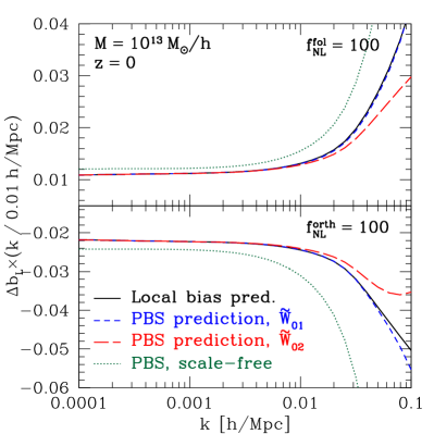
Figure 3: Same as Fig. 2, but for the folded (top) and orthogonal (bottom) models. We have taken out a scaling factor of $(k/0.01\,h~{}{\rm Mpc}^{-1})^{-1}$.

VI Peak-background split vs. local biasing

The effects on the halo power spectrum from non-local non-Gaussianity have also been derived in a local-Lagrangian-biasing (LLB) scheme Verde:2009hy ; Matarrese:1986et . In this approach, halos are identified with high-density regions in the initial non-Gaussian density field. Specifically, the density $\delta_{R}$ smoothed on a scale $R$ (again related to the halo mass by $M=4\pi/3\overline{\rho}R^{3}$) is required to be greater than the linear collapse threshold $\delta_{c}$. This is equivalent to a local-biasing scheme relating the halo density field $\delta_{h}$ to the smoothed (non-Gaussian) matter density field:

$$\delta_{h}(\mathbf{x})=b_{L}\hat{\delta}_{R}(\mathbf{x})+\frac{b_{L,2}}{2}\hat{\delta}_{R}^{2}(\mathbf{x})+\dots,$$ (63)

where $b_{L,2}$ is the second-order Lagrangian bias. In the high-peak limit which we will assume here, $b_{L}=\delta_{c}/\sigma_{R}^{2}$, and $b_{L,2}=b_{L}^{2}$ (see discussion below).

Since primordial non-Gaussianity induces a non-zero three-point function in the density field, the large-scale halo correlation function is modified to

$$\xi_{h}(r)=b_{L}^{2}\xi_{R}(r)+b_{L}\>b_{L,2}\>\xi_{R}^{(3)}(\mathbf{x}_{1},\mathbf{x}_{1},\mathbf{x}_{2}),$$ (64)

where $\xi_{R}$ and $\xi_{R}^{(3)}$ denote the two- and three-point functions of the smoothed density field, respectively. Note that, again, the three-point correlation function is evaluated in the squeezed limit. In Fourier space, this reads Schmidt:2010pf

$$P_{h}(k)=\; b_{L}^{2}P_{R}(k)+b_{L}\>b_{L,2}\>\mathscr{p}^{\delta\delta\delta}(k),$$ (65)

$$\mathscr{p}^{\delta\delta\delta}(k)=\; \int\frac{{\rm d}^{3}\mathbf{k}_{1}}{(2\pi)^{3}}B_{R}(k,k_{1},|\mathbf{k}_{1}-\mathbf{k}|).$$ (66)

Here, $P_{R}(k)\equiv F_{R}^{2}(k)P(k)$, and correspondingly for the bispectrum $B_{R}$. Note that in this approach the correction to the halo power spectrum comes about from the quadratic bias parameter. With this, we can write the effective correction to the linear halo bias as

$$\Delta b_{L}(k)=\frac{1}{2}b_{L,2}\frac{\mathscr{p}^{\delta\delta\delta}(k)}{P_{R}(k)}=b_{L}\delta_{c}\frac{1}{2\sigma_{R}^{2}}\frac{\mathscr{p}^{\delta\delta\delta}(k)}{P_{R}(k)},$$ (67)

where for the second equality we have assumed the high-peak limit. We show the predictions of the local-bias model in Fig. 2 for the equilateral and SOSF models. We see that on the largest scales, the peak-background split prediction agrees precisely with that of local biasing. On the other hand, on intermediate scales $k\gtrsim 0.01\,h~{}{\rm Mpc}^{-1}$, the two approaches begin to diverge, with the peak-background split generally predicting lower halo bias corrections. We will now show how this comes about.

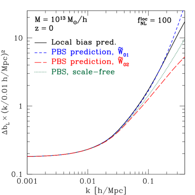
Figure 4: Same as Fig. 2, but now for the local model. We have taken out a scaling of $(k/0.01\,h~{}{\rm Mpc}^{-1})^{-2}$ here.

We can write the bias correction in both the PBS and LLB schemes as (see also DesjacquesSeljak )

$$\Delta b_{L}(k)=2f_{\rm NL}b_{L}\delta_{c}\sigma_{R}^{-2}\mathcal{F}(k),$$ (68)

with

$$\mathcal{F}^{\rm PBS}(k)=\; \frac{1}{\mathcal{M}(k)F_{R}(k)}\int\frac{d^{3}k_{1}}{(2\pi)^{3}}P_{R}(k_{1})\widetilde{W}_{0}(\mathbf{k},\mathbf{k}_{1}-\mathbf{k}),$$ (69)

$$\mathcal{F}^{\rm LLB}(k)=\; \frac{1}{4f_{\rm NL}P_{R}(k)}\int\frac{{\rm d}^{3}\mathbf{k}_{1}}{(2\pi)^{3}}B_{R}(k,k_{1},|\mathbf{k}_{1}-\mathbf{k}|).$$ (70)

The additional $F_{R}^{-1}$ prefactor in $\mathcal{F}^{\rm PBS}$ is necessary to match the local-biasing prediction, since the latter refers the halo bias to the smoothed density field [Eq. (63)]: doing the same in the PBS approach, via Eq. (IV), Eq. (39) and using $\tilde{\delta}_{R}=F_{R}\tilde{\delta}$, results in this prefactor.

We now insert the definition of $\widetilde{W}_{0}$ [Eq. (21) or Eq. (22)] into Eq. (69), and use the relation between the smoothed density field and potential,

$$P_{R}(k)=\; \mathcal{M}_{R}^{2}(k)P_{\Phi_{0}}(k),$$

$$B_{R}(k_{1},k_{2},k_{3})=\; \mathcal{M}_{R}(k_{1})\mathcal{M}_{R}(k_{2})\mathcal{M}_{R}(k_{3})B_{\Phi_{0}}(k_{1},k_{2},k_{3}),$$

where we have defined $\mathcal{M}_{R}(k)\equiv\mathcal{M}(k)F_{R}(k)$. It is then straightforward to show that

$$\mathcal{F}^{\rm PBS}(k)=\; \frac{1}{4f_{\rm NL}P_{R}(k)}\int\frac{{\rm d}^{3}\mathbf{k}_{1}}{(2\pi)^{3}}B_{R}(k,k_{1},|\mathbf{k}_{1}-\mathbf{k}|)$$

$$\times A(\mathbf{k},\mathbf{k}_{1})\>C(\mathbf{k},\mathbf{k}_{1}),$$ (71)

where

$$A(\mathbf{k},\mathbf{k}_{1})=\; \frac{\mathcal{M}_{R}(k_{1})}{\mathcal{M}_{R}(|\mathbf{k}_{1}-\mathbf{k}|)}=\frac{k_{1}^{2}}{|\mathbf{k}_{1}-\mathbf{k}|^{2}}\frac{F_{R}(k_{1})}{F_{R}(|\mathbf{k}_{1}-\mathbf{k}|)},$$ (72)

and

$$C_{1}(\mathbf{k},\mathbf{k}_{1})=\; 2\frac{T^{2}(k_{1})}{T^{2}(|\mathbf{k}_{1}-\mathbf{k}|)}$$

$$\times\left(1+\frac{P_{\Phi}(|\mathbf{k}_{1}-\mathbf{k}|)}{P_{\Phi}(k_{1})}+\frac{P_{\Phi}(|\mathbf{k}_{1}-\mathbf{k}|)}{P_{\Phi}(k)}\right)^{-1},$$ (73)

(note that $P_{\Phi}$ is the power spectrum for the primordial potential) if we use $\widetilde{W}_{01}$ for the processed kernel, and

$$C_{2}(\mathbf{k},\mathbf{k}_{1})=\; 2\left(1+\frac{P_{\Phi_{0}}(|\mathbf{k}_{1}-\mathbf{k}|)}{P_{\Phi_{0}}(k_{1})}+\frac{P_{\Phi_{0}}(|\mathbf{k}_{1}-\mathbf{k}|)}{P_{\Phi_{0}}(k)}\right)^{-1},$$ (74)

(and here $P_{\Phi_{0}}$ is the power spectrum for the processed potential) if we use $\widetilde{W}_{02}$ for the processed kernel.

In the true squeezed limit, $q=k/k_{1}$ becomes negligible, so that $A\rightarrow 1$ and $C_{1}\rightarrow 1$ and $C_{2}\rightarrow 1$ (the second term in the brackets for both expressions becomes 1, while the last term vanishes in this limit). Clearly, $\mathcal{F}^{\rm PBS}=\mathcal{F}^{\rm loc}$ in this limit, which explains why both approaches agree on large scales. Going back to Eq. (69), we see that the integrand peaks where $P_{R}(k_{1})$ peaks, roughly around $k_{1}\sim 0.02\,h~{}{\rm Mpc}^{-1}$. Furthermore, as $k_{1}$ becomes comparable to $k$, $|\mathbf{k}_{1}-\mathbf{k}|$ can assume values much smaller than $k_{1}$. Thus, we expect that deviations of $\mathcal{F}^{\rm PBS}$ from $\mathcal{F}^{\rm LLB}$ appear at least around $k\sim 0.01\,h~{}{\rm Mpc}^{-1}$, which indeed is visible in Fig. 2. Similar but somewhat smaller deviations occur in the folded and orthogonal cases (Fig. 3), and even in the local model of non-Gaussianity (see Fig. 4). Hence, the agreement between the PBS and LLB approaches is restricted to the largest scales in the well-studied local model as well. However, since the halo-bias correction strongly declines towards smaller scales, the deviations between the two approaches have much less impact in the local model. We have confirmed numerically that by introducing the correction factors $A^{-1}$ and $C^{-1}$ into the PBS expression Eq. (47), we recover the LLB prediction exactly.

On a more physical level, the differences in scale-dependence between the PBS and LLB predictions come from the assumption of a separation of scales between the large-scale modes modulating the clustering of halos, and the small-scale modes that govern their formation. In the course of this assumption, several terms in the relation between short-wavelength and long-wavelength perturbations have been neglected (see § III). This assumption breaks down on smaller scales, however; modes with $k\sim 0.01\,h~{}{\rm Mpc}^{-1}$, for example, contribute significantly to the density variance $\sigma_{R}^{2}$, and if we want to calculate the clustering of halos at that $k$, the separation of scales does not hold anymore. On the other hand, no such assumption of separation of scales is made in the LLB approach. Here, the assumption is that halo formation is purely a function of the local physical density. Of course, both approaches need to be benchmarked with simulations Wagner:2010me in the end, which will have the final say on the scaling of the halo bias in models with non-local non-Gaussianity.

Even on large scales, there is a difference between the PBS and LLB predictions: in the PBS approach, $\Delta b\propto\sigma_{R}^{-2}\partial\ln n/\partial\ln\sigma_{R}$, which for any universal mass function equals $b_{L}\delta_{c}/\sigma_{R}^{2}$. On the other hand, LLB predicts that $\Delta b\propto b_{L,2}$. While this agrees with the PBS prediction in the high-peak limit of the Press-Schechter theory, where $b_{L,2}=b_{L}^{2}=b_{L}\delta_{c}/\sigma_{R}^{2}$, this is not the case in general. For example, the quadratic bias derived from the Sheth-Tormen mass function Sheth:1999mn in the high-peak limit is $b_{L,2}=q\>b_{L}\delta_{c}/\sigma_{R}^{2}$, thus deviating from $\sigma_{R}^{-2}\partial\ln n/\partial\ln\sigma_{R}$ by a factor of $q\approx 0.75$. This number will be different in other mass function prescriptions. Also, the quadratic bias parameter has to change sign at a finite $\nu$, while $b_{L}\delta_{c}/\sigma_{R}^{2}$ is always positive. Hence, outside of the high-peak limit the differences between LLB and PBS predictions can become larger. It is worth pointing out that since there is no prescription for small-scale physics contained in the local biasing approach, there is no analogous expression or prediction for the quantity $\partial\ln n/\partial\sigma_{R}$. In the end, a comparison with simulations will have to determine whether the non-Gaussian bias correction follows a scaling with $\partial\ln n/\partial\sigma_{R}$, as predicted by the PBS, or with the quadratic bias $b_{L,2}$, as predicted by local biasing — both of these predictions are falsifiable.

VII Conclusions

The principal goal of the theory of large-scale structure is to map the initial linear density field into the late-time non-linear matter density. One of the most fascinating recent applications of this theory is the effect of primordial non-Gaussianity on the clustering of dark matter halos. Here, we derived predictions for general quadratic non-Gaussianity in the peak-background-split (PBS) approach, focusing on the case of universal halo mass functions. This complements the derivation of Ref. Verde:2009hy in the local-bias model. We also show how the non-Gaussian effect on halo bias can be calculated beyond universal mass functions, by taking into account all dependences of the halo abundance on the statistics of small-scale fluctuations [Eq. (LABEL:eq:Db-1)].

While we have only considered general quadratic non-Gaussianity here, it is possible to generalize these results to the case of cubic non-Gaussianity, described by the trispectrum rather than the bispectrum of primordial fluctuations. For example, for the local cubic model, we expect the non-Gaussian halo bias to scale as $\sim k^{-2}$ like in the local quadratic model DesjacquesSeljak10b . A detailed investigation of cubic non-Gaussianity is beyond the scope of this paper however.

We show that both PBS and local bias approaches agree in their predictions on large scales, $k\lesssim 0.01\,h~{}{\rm Mpc}^{-1}$, when the high-peak limit is assumed in the local bias approach, but predictions diverge on smaller scales. The disagreement comes about from the breakdown of the separation-of-scales assumption inherent in the PBS approach. Even on large scales, however, both approaches do not in general agree: in the PBS approach (with a universal mass function), the non-Gaussian effect on the halo bias scales with $\partial\ln n/\partial\sigma_{R}=b_{L}\delta_{c}/\sigma_{R}$, which quantifies the dependence of the halo number on the variance of the small-scale fluctuations. By the nature of the approach, there is no analogous quantity in the local bias framework. Here, the halo bias correction scales with the quadratic bias parameter $b_{L,2}$ which in general is not directly related to $\partial\ln n/\partial\sigma_{R}$. This disagreement will also have consequences for predictions of higher order statistics (e.g., the bispectrum) of halos, where both $b_{L,2}$ and the non-Gaussian bias contribution appear.

N-body simulations will have the final say on which of the two approaches has the right scaling with halo mass (or equivalently, significance $\nu$), and with scale; it is possible that PBS fares better in the former respect, while LLB is closer to reality in the latter.

Appendix A The local-model bispectrum from a nonlocal model

In § II, we showed that the bispectrum $B_{\Phi}(k_{1},k_{2},k_{3})$ does not uniquely determine the kernel $\widetilde{W}(\mathbf{k}_{1},\mathbf{k}_{2})$. Several different kernels may give rise to the same bispectrum. We moreover constructed explicitly two different processed kernels $\widetilde{W}_{0}(\mathbf{k}_{1},\mathbf{k}_{2})$ for a given bispectrum. Let us now use Eq. (22) for the processed kernel for the (processed) bispectrum for the local model. If we then invert Eq. (17) to obtain the primordial kernel that corresponds to this processed kernel, we find,

$$\widetilde{W}(\mathbf{k}_{1},\mathbf{k}_{2})=\frac{\left[T(k_{1})T(k_{2})\right]^{2}(P_{1}P_{2}+2\,\mathrm{perms})}{\left[T(k_{1})T(k_{2})\right]^{2}P_{1}P_{2}+2\,\mathrm{perms}}.$$ (75)

Upon substituting into Eq. (5), we recover the local-model bispectrum, Eq. (7).

Moreover, the function $T(k)$ that appears in Eq. (75) need not be the transfer function for the local-model bispectrum to be recovered. Indeed, any kernel,

$$\widetilde{W}(\mathbf{k}_{1},\mathbf{k}_{2})=\frac{\left[f(k_{1})f(k_{2})\right]^{2}(P_{1}P_{2}+2\,\mathrm{perms})}{\left[f(k_{1})f(k_{2})\right]^{2}P_{1}P_{2}+2\,\mathrm{perms}},$$ (76)

for any function $f(k)$ will yield the local-model bispectrum. And for any function $f(k)$ that is not simply a constant, the configuration-space kernel $W(\mathbf{y},\mathbf{z})$ obtained through the inverse transform of Eq. (3) will be nonlocal.

In fact, the ambiguity in the kernel $\widetilde{W}$ is much more general: for any positive function of three arguments, $g(k_{1},k_{2},k_{3})$, and any bispectrum $B_{\Phi}$, we can construct a kernel satisfying Eq. (5):

$$\widetilde{W}(k_{1},k_{2},k_{3})=\> \frac{g(k_{1},k_{2},k_{3})}{g(k_{1},k_{2},k_{3})P_{1}P_{2}+2\,\mathrm{perms}}$$

$$\>\times\frac{B_{\Phi}(k_{1},k_{2},k_{3})}{2f_{\rm NL}}.$$ (77)

We have therefore shown, by explicit construction, that there are models in which the potential $\Phi$ is a nonlocal quadratic function of a Gaussian field $\phi$ that have the same bispectrum as that for the local model. We therefore conclude that measurement of the local-model bispectrum does not necessarily imply that the potential has the local-model form given in Eq. (10). Note, though, that these different models may still differ in their predicted $\mathcal{O}(f_{\rm NL}^{2})$ trispectra. For now, we treat this simply as a mathematical curiosity, and we leave the investigation of the implications of this result for model building for future work.

References

- (1) F. Bernardeau, S. Colombi, E. Gaztanaga and R. Scoccimarro, Phys. Rept. 367, 1 (2002) [arXiv:astro-ph/0112551].
- (2) A. H. Guth and S. Y. Pi, Phys. Rev. Lett. 49, 1110 (1982); A. A. Starobinsky, Phys. Lett. B 117, 175 (1982); J. M. Bardeen, P. J. Steinhardt and M. S. Turner, Phys. Rev. D 28, 679 (1983).
- (3) N. Bartolo et al., Phys. Rept. 402, 103 (2004) [arXiv:astro-ph/0406398];
- (4) T. Falk, R. Rangarajan and M. Srednicki, Astrophys. J. 403, L1 (1993) [arXiv:astro-ph/9208001]; A. Gangui et al., Astrophys. J. 430, 447 (1994) [arXiv:astro-ph/9312033]; A. Gangui, Phys. Rev. D 50, 3684 (1994) [arXiv:astro-ph/9406014]; L. M. Wang and M. Kamionkowski, Phys. Rev. D 61, 063504 (2000) [arXiv:astro-ph/9907431]; J. M. Maldacena, JHEP 0305, 013 (2003) [arXiv:astro-ph/0210603]; V. Acquaviva, N. Bartolo, S. Matarrese and A. Riotto, Nucl. Phys. B 667, 119 (2003) [arXiv:astro-ph/0209156].
- (5) T. J. Allen, B. Grinstein and M. B. Wise, Phys. Lett. B 197, 66 (1987); L. A. Kofman and D. Y. Pogosian, Phys. Lett. B 214, 508 (1988); D. S. Salopek, J. R. Bond and J. M. Bardeen, Phys. Rev. D 40, 1753 (1989); A. D. Linde and V. F. Mukhanov, Phys. Rev. D 56, 535 (1997) [arXiv:astro-ph/9610219]; P. J. E. Peebles, Astrophys. J. 510, 523 (1999) [arXiv:astro-ph/9805194]; P. J. E. Peebles, Astrophys. J. 510, 531 (1999) [arXiv:astro-ph/9805212].
- (6) S. Mollerach, Phys. Rev. D 42, 313 (1990); A. D. Linde and V. F. Mukhanov, Phys. Rev. D 56, 535 (1997) [arXiv:astro-ph/9610219]; D. H. Lyth and D. Wands, Phys. Lett. B 524, 5 (2002) [arXiv:hep-ph/0110002]; K. Enqvist and M. S. Sloth, Nucl. Phys. B 626, 395 (2002); T. Moroi and T. Takahashi, Phys. Lett. B 522, 215 (2001) [Erratum-ibid. B 539, 303 (2002)] [arXiv:hep-ph/0110096]; D. H. Lyth, C. Ungarelli and D. Wands, Phys. Rev. D 67, 023503 (2003) [arXiv:astro-ph/0208055]; K. Ichikawa et al., arXiv:0802.4138 [astro-ph]; K. Enqvist, S. Nurmi, O. Taanila and T. Takahashi, arXiv:0912.4657 [astro-ph.CO]; K. Enqvist and T. Takahashi, JCAP 0912, 001 (2009) [arXiv:0909.5362 [astro-ph.CO]]; K. Enqvist and T. Takahashi, JCAP 0809, 012 (2008) [arXiv:0807.3069 [astro-ph]]; K. Enqvist and S. Nurmi, JCAP 0510, 013 (2005) [arXiv:astro-ph/0508573]; A. L. Erickcek, M. Kamionkowski and S. M. Carroll, arXiv:0806.0377 [astro-ph]; A. L. Erickcek, C. M. Hirata and M. Kamionkowski, Phys. Rev. D 80, 083507 (2009) [arXiv:0907.0705 [astro-ph.CO]]; S. Hannestad, T. Haugboelle, P. R. Jarnhus and M. S. Sloth, arXiv:0912.3527 [hep-ph].
- (7) G. R. Dvali and S. H. H. Tye, Phys. Lett. B 450, 72 (1999) [arXiv:hep-ph/9812483]; P. Creminelli, JCAP 0310, 003 (2003) [arXiv:astro-ph/0306122]; M. Alishahiha, E. Silverstein and D. Tong, Phys. Rev. D 70, 123505 (2004) [arXiv:hep-th/0404084].
- (8) A. Vilenkin and E. P. S. Shellard “Cosmic Strings and other Topological Defects,” (Cambridge University Press, Cambridge, 1994); R. Durrer, New Astron. Rev. 43, 111 (1999); R. Durrer, M. Kunz and A. Melchiorri, Phys. Rept. 364, 1 (2002) [arXiv:astro-ph/0110348]; A. H. Jaffe, Phys. Rev. D 49, 3893 (1994) [arXiv:astro-ph/9311023]; A. Silvestri and M. Trodden, Phys. Rev. Lett. 103, 251301 (2009) [arXiv:0811.2176 [astro-ph]]; M. Hindmarsh, C. Ringeval and T. Suyama, Phys. Rev. D 80, 083501 (2009) [arXiv:0908.0432 [astro-ph.CO]]; M. Hindmarsh, C. Ringeval and T. Suyama, arXiv:0911.1241 [astro-ph.CO]; D. M. Regan and E. P. S. Shellard, arXiv:0911.2491 [astro-ph.CO]; N. Turok and D. N. Spergel, Phys. Rev. Lett. 66, 3093 (1991).
- (9) D. G. Figueroa, R. R. Caldwell and M. Kamionkowski, arXiv:1003.0672 [astro-ph.CO].
- (10) W. A. Chiu, J. P. Ostriker and M. A. Strauss, Astrophys. J. 494, 479 (1998) [arXiv:astro-ph/9708250]; J. Robinson, E. Gawiser and J. Silk, Astrophys. J. 532, 1 (2000) [arXiv:astro-ph/9906156]; J. A. Willick, Astrophys. J. 530, 80 (2000) [arXiv:astro-ph/9904367]; L. Verde et al., Mon. Not. Roy. Astron. Soc. 321, L7 (2001) [arXiv:astro-ph/0007426]; N. N. Weinberg and M. Kamionkowski, Mon. Not. Roy. Astron. Soc. 341, 251 (2003) [arXiv:astro-ph/0210134]; S. Matarrese, L. Verde and R. Jimenez, Astrophys. J. 541, 10 (2000) [arXiv:astro-ph/0001366]; L. Verde et al., Mon. Not. Roy. Astron. Soc. 325, 412 (2001) [arXiv:astro-ph/0011180]; M. LoVerde et al., JCAP 0804, 014 (2008) [arXiv:0711.4126 [astro-ph]]; L. Cayon, C. Gordon and J. Silk, arXiv:1006.1950 [astro-ph.CO]; S. Sadeh, Y. Rephaeli and J. Silk, Mon. Not. Roy. Astron. Soc. 380, 637 (2007) [arXiv:0706.1340 [astro-ph]]; M. Kamionkowski, L. Verde and R. Jimenez, JCAP 0901, 010 (2009) [arXiv:0809.0506 [astro-ph]]; S. Chongchitnan and J. Silk, arXiv:1007.1230 [astro-ph.CO]; G. D’Amico, et al., arXiv:1005.1203 [astro-ph.CO].
- (11) L. Verde, M. Kamionkowski, J. J. Mohr and A. J. Benson, Mon. Not. Roy. Astron. Soc. 321, L7 (2001) [arXiv:astro-ph/0007426].
- (12) P. Coles et al., Mon. Not. Roy. Astron. Soc. 264, 749 (1993) [arXiv:astro-ph/9302015]; X. c. Luo and D. N. Schramm, Astrophys. J. 408, 33 (1993); E. Lokas et al., Mon. Not. Roy. Astron. Soc. 274, 730 (1995) [arXiv:astro-ph/9407095]; M. J. Chodorowski and F. R. Bouchet, Mon. Not. Roy. Astron. Soc. 279, 557 (1996) [arXiv:astro-ph/9507038]; A. J. Stirling and J. A. Peacock, Mon. Not. Roy. Astron. Soc. 283, 99 (1996) [arXiv:astro-ph/9608101]; R. Durrer et al., Phys. Rev. D 62, 021301 (2000) [arXiv:astro-ph/0005087]. L. Verde and A. F. Heavens, Astrophys. J. 553, 14 (2001) [arXiv:astro-ph/0101143]; A. Buchalter and M. Kamionkowski, Astrophys. J. 521, 1 (1999) [arXiv:astro-ph/9903462]; A. Buchalter, M. Kamionkowski and A. H. Jaffe, Astrophys. J. 530, 36 (2000) [arXiv:astro-ph/9903486].
- (13) L. Verde et al., Mon. Not. Roy. Astron. Soc. 313, L141 (2000) [arXiv:astro-ph/9906301]; E. Komatsu and D. N. Spergel, Phys. Rev. D 63, 063002 (2001) [arXiv:astro-ph/0005036].
- (14) E. Komatsu et al. [WMAP Collaboration], Astrophys. J. Suppl. 148, 119 (2003) [arXiv:astro-ph/0302223]; A. P. S. Yadav and B. D. Wandelt, Phys. Rev. Lett. 100, 181301 (2008) [arXiv:0712.1148 [astro-ph]]; E. Komatsu et al. [WMAP Collaboration], Astrophys. J. Suppl. 180, 330 (2009) [arXiv:0803.0547 [astro-ph]]; P. Creminelli, A. Nicolis, L. Senatore, M. Tegmark and M. Zaldarriaga, JCAP 0605, 004 (2006) [arXiv:astro-ph/0509029].
- (15) E. Komatsu et al., arXiv:1001.4538 [astro-ph.CO].
- (16) N. Dalal, O. Dore, D. Huterer and A. Shirokov, Phys. Rev. D 77, 123514 (2008) [arXiv:0710.4560 [astro-ph]].
- (17) A. Slosar, C. Hirata, U. Seljak, S. Ho and N. Padmanabhan, JCAP 0808, 031 (2008) [arXiv:0805.3580 [astro-ph]].
- (18) T. Giannantonio and C. Porciani, Phys. Rev. D 81, 063530 (2010) [arXiv:0911.0017 [astro-ph.CO]].
- (19) S. Matarrese and L. Verde, Astrophys. J. 677, L77 (2008) [arXiv:0801.4826 [astro-ph]]; C. Carbone, L. Verde and S. Matarrese, Astrophys. J. 684, L1 (2008) [arXiv:0806.1950 [astro-ph]].
- (20) V. Desjacques and U. Seljak, arXiv:1006.4763 [astro-ph.CO].
- (21) J. Q. Xia, M. Viel, C. Baccigalupi, G. De Zotti, S. Matarrese and L. Verde, arXiv:1003.3451 [astro-ph.CO]; J. Q. Xia, A. Bonaldi, C. Baccigalupi, G. De Zotti, S. Matarrese, L. Verde and M. Viel, arXiv:1007.1969 [astro-ph.CO].
- (22) L. Verde and S. Matarrese, Astrophys. J. 706, L91 (2009) [arXiv:0909.3224 [astro-ph.CO]].
- (23) S. Matarrese, F. Lucchin and S. A. Bonometto, Astrophys. J. 310, L21 (1986).
- (24) P. Catelan, C. Porciani and M. Kamionkowski, Mon. Not. Roy. Astron. Soc. 318, 39 (2000) [arXiv:astro-ph/0005544].
- (25) D. Babich, P. Creminelli and M. Zaldarriaga, JCAP 0408, 009 (2004) [arXiv:astro-ph/0405356]; P. Creminelli et al., JCAP 0605, 004 (2006) [arXiv:astro-ph/0509029]; P. Creminelli et al., JCAP 0703, 005 (2007) [arXiv:astro-ph/0610600].
- (26) X. Chen, M. x. Huang, S. Kachru and G. Shiu, JCAP 0701, 002 (2007) [arXiv:hep-th/0605045]; X. Chen, R. Easther and E. A. Lim, JCAP 0706, 023 (2007) [arXiv:astro-ph/0611645]; R. Holman and A. J. Tolley, JCAP 0805, 001 (2008) [arXiv:0710.1302 [hep-th]]; P. D. Meerburg, J. P. van der Schaar and P. S. Corasaniti, JCAP 0905, 018 (2009) [arXiv:0901.4044 [hep-th]].
- (27) L. Senatore, K. M. Smith and M. Zaldarriaga, JCAP 1001, 028 (2010) [arXiv:0905.3746 [astro-ph.CO]].
- (28) X. c. Luo, Astrophys. J. 427, L71 (1994) [arXiv:astro-ph/9312004].
- (29) W. H. Press and P. Schechter, Astrophys. J. 187, 425 (1974); R. K. Sheth, H. J. Mo and G. Tormen, Mon. Not. Roy. Astron. Soc. 323, 1 (2001) [arXiv:astro-ph/9907024].
- (30) H. J. Mo and S. D. M. White, Mon. Not. Roy. Astron. Soc. 282, 347 (1996) [arXiv:astro-ph/9512127].
- (31) R. K. Sheth and G. Tormen, Mon. Not. Roy. Astron. Soc. 308, 119 (1999) [arXiv:astro-ph/9901122].
- (32) F. Schmidt, arXiv:1005.4063 [astro-ph.CO].
- (33) C. Wagner, L. Verde and L. Boubekeur, arXiv:1006.5793 [astro-ph.CO].
- (34) V. Desjacques and U. Seljak, Phys. Rev. D 81, 023006 (2010) arXiv:0907.2257 [astro-ph.CO].