X-ray emission from the Sombrero galaxy: discrete sources

Abstract

We present a study of discrete X-ray sources in and around the bulge-dominated, massive Sa galaxy, Sombrero (M104), based on new and archival Chandra observations with a total exposure of $\sim$200 ks. With a detection limit of $L_{\rm X}\approx 10^{37}{\rm~{}ergs~{}s^{-1}}$ and a field of view covering a galactocentric radius of $\sim$30 kpc (11$\farcm$5), 383 sources are detected. Cross-correlation with Spitler et al.’s catalogue of Sombrero globular clusters (GCs) identified from HST/ACS observations reveals 41 X-rays sources in GCs, presumably low-mass X-ray binaries (LMXBs). Metal-rich GCs are found to have a higher probability of hosting these LMXBs, a trend similar to that found in elliptical galaxies. On the other hand, the four most luminous GC LMXBs, with apparently super-Eddington luminosities for an accreting neutron star, are found in metal-poor GCs. We quantify the differential luminosity functions (LFs) for both the detected GC and field LMXBs, whose power-low indices ($\sim$1.1 for the GC-LF and $\sim$1.6 for field-LF) are consistent with previous studies for elliptical galaxies. With precise sky positions of the GCs without a detected X-ray source, we further quantify, through a fluctuation analysis, the GC LF at fainter luminosities down to $10^{35}{\rm~{}ergs~{}s^{-1}}$. The derived index rules out a faint-end slope flatter than 1.1 at a 2 $\sigma$ significance, contrary to recent findings in several elliptical galaxies and the bulge of M31. On the other hand, the 2-6 keV unresolved emission places a tight constraint on the field LF, implying a flattened index of $\sim$1.0 below $10^{37}{\rm~{}ergs~{}s^{-1}}$. We also detect 101 sources in the halo of Sombrero. The presence of these sources cannot be interpreted as galactic LMXBs whose spatial distribution empirically follows the starlight. Their number is also higher than the expected number of cosmic AGNs ($52\pm 11$ [1 $\sigma$]) whose surface density is constrained by deep X-ray surveys. We suggest that either the cosmic X-ray background is unusually high in the direction of Sombrero, or a distinct population of X-ray sources is present in the halo of Sombrero.

1 Introduction

The Chandra X-ray Observatory, with its superb angular resolution and sensitivity, has established the ubiquity of LMXBs in nearby early-type galaxies (e.g., Sarazin et al. 2000; Kraft et al. 2001), in particular confirming the hypothesis that such a population accounts for the bulk of X-ray emission in X-ray-faint elliptical/S0 galaxies (i.e., galaxies with a low $L_{X}/L_{B}$ ratio). The total number and cumulative luminosity of LMXBs are further shown to be good indicators of the host galaxy’s stellar mass (Gilfanov 2004), with only a weak dependence on morphological type. This dependence is at least partly related to the specific frequency of GCs in which LMXBs are efficiently formed through dynamical processes (Clark 1975).

Chandra observations of more than a dozen nearby elliptical/S0 galaxies have provided valuable information on their LMXB populations (Kim et al. 2006; Kundu, Maccarone & Zepf 2007; Sivakoff et al. 2008; Brassington et al. 2008, 2009; Posson-Brown et al. 2009; Voss et al. 2009; Kim et al. 2009, among many recent studies). However, a comparative view for bulges of spiral galaxies is still limited. Our present knowledge comes primarily from LMXBs detected in M31 (Kong et al. 2002; Voss & Gilfanov 2007), M81 (Tennant et al. 2001), M104 (Di Stefano et al. 2003) and our own Galaxy. Since observations of elliptical/S0 galaxies rarely reach a source detection limit below $10^{37}{\rm~{}ergs~{}s^{-1}}$, LMXBs with luminosities as low as $10^{35}$-$10^{36}{\rm~{}ergs~{}s^{-1}}$ are chiefly detected in the bulges of M31 and our Galaxy. However, the number of LMXBs in these two bulges is limited by their moderate stellar mass and their relatively low specific GC frequency. Sensitive X-ray studies of nearby bulges can improve our knowledge of the LMXB population in this important galactic component.

The Sombrero galaxy (M104; NGC 4594), a bulge-dominated, edge-on Sa galaxy at a distance of 9.0$\pm$0.1 Mpc (Spitler et al. 2006), has a total stellar mass comparable to that of the most massive elliptical galaxies in the Virgo cluster. The galaxy also harbors a sizable population of GCs, with an estimated number of $\sim$2000 (Rhode & Zepf 2004). Therefore a large number of LMXBs is expected in Sombrero, making it an ideal target for studying both sources residing in the GCs and in the field. Indeed, in a shallow Chandra observation of Sombrero, Di Stefano et al. (2003) found more than 100 discrete sources. Two deep Chandra observations were recently taken, effectively adding Sombrero to a short list of early-type galaxies for which a source detection limit below $10^{37}{\rm ergs~{}s^{-1}}$ is achieved. In this work we study the stellar populations, mostly LMXBs, based on these observations. In a forthcoming paper we will present a study of the diffuse X-ray emission.

In § 2 we briefly describe the data preparation. We present our analysis in § 3 and discuss the results in § 4. A summary is given in § 5. We quote 1 $\sigma$ errors throughout this work.

2 Data preparation

2.1 X-ray and optical data

Existing Chandra studies of X-ray sources in Sombrero (Di Stefano et al. 2003; Kundu et al. 2007; Li, Wang & Hameed 2007) are based on a 19-ks ACIS-S observation taken on May 31, 2001 (Obsid. 1586; PI: S. Murray). On April 29 and December 2, 2008, we obtained two new Chandra ACIS-I observations (Obsid. 9532 and 9533; PI: C. Jones), with exposures of 85 and 90 ks, respectively. In this work we utilize data from all three observations. We reprocessed the data using CIAO v.4.1 and the corresponding calibration files, following the Chandra ACIS data analysis guide. No time intervals of high particle background were found. We calibrated the relative astrometry among the three observations using the CIAO tool reproject_aspect, by matching centroids of discrete sources commonly detected in all three observations. The resultant relative astrometry is better than 0$\farcs$1. For each observation, we produced count and exposure maps in the 0.4-0.7 (S1), 0.7-1 (S2), 1-2 (H1) and 2-6 (H2) keV bands. An absorbed power-law spectrum, with a photon-index of 1.7 and an absorption column density $N_{\rm H}=10^{21}{\rm~{}cm^{-2}}$ (a value somewhat higher than the Galactic foreground column density toward Sombrero, $3.7{\times}10^{20}{\rm~{}cm^{-2}}$ [Dickey & Lockman 1990], but allowing for some internal absorption), was adopted to calculate spectral weights when producing the exposure maps. The energy-dependent difference of effective area between the ACIS-S3 CCD and the ACIS-I CCDs was taken into account, assuming the above incident spectrum, so that the quoted count rates throughout this work refer to ACIS-I. The count and exposure maps of individual observations were projected to a common tangential point, here the optical center of Sombrero, to produce summed images of the combined field of view (FoV; Fig. 1a). The total effective exposure, in the 2-6 keV band for example, is $\gtrsim$180 ks within a projected galactocentric radius $R\approx 4^{\prime}$, where the FoV is common to the three observations, and gradually drops below 80 ks at $R\gtrsim 8^{\prime}$.

Hubble Space Telescope (HST) Advance Camera for Surveys (ACS) data in the “science-ready form” were used by Spitler et al. (2006; hereafter S06) to identify GC candidates in a $\sim$600${}^{\prime\prime}\times 400^{\prime\prime}$ 6-pointing mosaic centered on Sombrero. Three optical bands ($BVR$) were obtained through the Hubble Heritage Project (PI: K. Noll, PID. 9714). S06 used photometric and size-selection (GCs are partially-resolved on the ACS imaging) to construct a catalogue of 659 GC candidates. Owing to the excellent quality of the HST images, the catalogue contains all but the faintest 5% of the GCs in this field, with minimal contamination. In particular, objects falling on Sombrero’s prominent dust lane are excluded. Here we use improved photometric measurements for the GC candidates (see discussion in Spitler, Forbes & Beasley 2008).

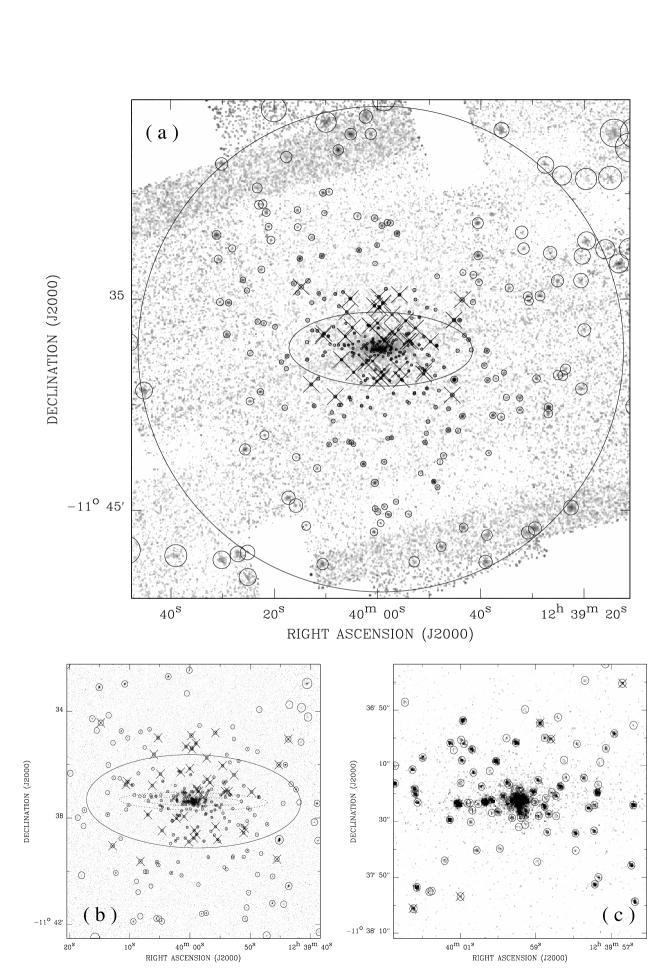
Figure 1: Smoothed 0.4-6 keV intensity images of M104 in (a) the 23^′ by 23^′ region. Detected X-ray sources are marked with circles of the 90% EER. GC sources are further marked with crosses. The ellipse (8$\farcm$7 by 3$\farcm$5) represents the $D_{25}$ isophote of the galaxy; the large circle encloses sources of interest; (b) the $10^{\prime}$ by $10^{\prime}$ region. The two dashed ellipses outline the dust lane; (c) the central 1$\farcm$5 by 1$\farcm$5 region.

2.2 X-ray source detection

Following the procedure detailed in Wang (2004), we detected sources in the soft (S1; 0.4-0.7 keV), medium (M=S2+H1; 0.7-2 keV), hard (H2; 2-6 keV) and full (F=S1+S2+H1+H2) bands. The low- and high-energy cut-offs were chosen to optimize the signal-to-noise ratio against the instrumental background. For the full combined FoV, a 2-pixel ($\sim$1^′′) binning was adopted to save computational effort; for the inner region ($R\lesssim$4^′), where source crowding is expected, the detection was refined using the original pixel scale ($\sim$0$\farcs$5/pixel). With a local false detection probability $P\leq 10^{-6}$ (yielding approximately one false source in the inner region and two false sources in the full FoV), we detected a total of 383 sources within $R$=11$\farcm$5 over the combined images (Fig. 1). Table 1 summarizes the detection results. For each source, background-subtracted, exposure map-corrected count rates in individual bands are derived from within the 90% enclosed energy radius (EER). We also calculated hardness ratios for each source using the method of Bayesian estimation (Park et al. 2006). In addition, we detected sources in individual observations to study long-term source variability (see § 3.5). Lists of sources detected in individual observations are summarized in Tables 2, 3 and 4.

To identify interlopers (e.g., relatively bright foreground stars and background galaxies), we rely on the USNO-B and 2MASS source catalogs (Monet et al. 2003; Cutri et al. 2003). A matching radius of 1^′′ is adopted, which yields random matches of 0.8 X-ray/optical pairs and 0.3 X-ray/near-infrared (NIR) pairs, under the assumption that interlopers are uniformly distributed within $R$=11$\farcm$5. In light of the intrinsic astrometry offset among the X-ray, optical and NIR source catalogs, we performed the matching procedure iteratively, in each run shifting the sky positions (R.A. and Dec.) of the optical (or NIR) sources by minimizing the cumulative position difference of the matched pairs, until the required shift is less than 0$\farcs$1. A total of 28 X-ray sources were thus identified as interlopers and excluded from further analysis. We also exclude the nucleus of Sombrero, the brightest source detected in the FoV (source 194 in Table 1). A detailed study of the nucleus will be given elsewhere. The remaining 354 sources are the subject of the analysis presented here.

The F-band count rates of individual sources are plotted against their galactocentric radii in Fig. 2, along with the radial variation of the detection threshold that depends on the local effective exposure, point spread function (PSF) and background. Across the FoV we achieve a minimum detection threshold of $8\times 10^{-5}{\rm~{}cts~{}s^{-1}}$ in the F-band, which corresponds to an intrinsic 0.5-8 keV luminosity of $\sim$$8\times 10^{36}{\rm~{}ergs~{}s^{-1}}$. Here we adopt an F-band count rate-to-flux conversion of $1.0\times 10^{-11}{\rm~{}ergs~{}s^{-1}~{}cm^{-2}}/({\rm cts~{}s^{-1}})$, or a F-band count rate-to-luminosity conversion of $9.7\times 10^{40}{\rm~{}ergs~{}s^{-1}}/({\rm cts~{}s^{-1}})$, for the assumed absorbed power-law model and distance of 9.0 Mpc (1^′=2.6 kpc) for Sombrero.

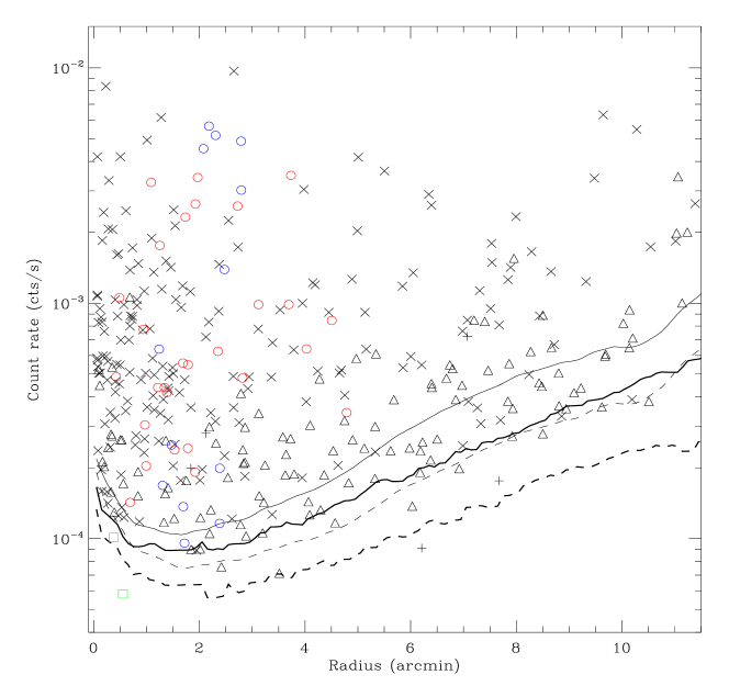
Figure 2:  0.4-6 keV (F-band) count rate vs. galactocentric radius for the detected sources. Red circle: sources associated with red GCs; blue circle: sources associated with blue GCs; green square: sources not detected in the M- and H2-bands; triangle: sources not detected in the S1- and H2-bands; plus: sources not detected in the S1- and M-bands; cross: sources detected in at least three bands. The solid and dashed curves illustrate the detection threshold in the F-band and M-band, respectively, with the thin one showing the azimuthal average value and the thick one showing the minimum value at each radius.

3 Analysis and results

3.1 X-ray sources associated with globular clusters

We begin our analysis by cross-correlating the detected X-ray sources with the GC catalogue of S06, with a similar procedure as we described above for the interlopers. A more conservative matching radius of 0$\farcs$5 is applied, for which 0.5 random matches are expected. This is estimated by artificially shifting the positions (R.A. and Dec.) of the X-ray sources by $\pm 5^{\prime\prime}$ and averaging the number of coincident matches. 41 pairs of GC-X-ray sources are identified (Fig. 1). Increasing the matching radius to 1^′′ results in 45 pairs, but accordingly $\sim$4 are expected to be random matches. Given their typical luminosities ($\gtrsim 10^{37}{\rm ergs~{}s^{-1}}$), these X-ray sources are most likely LMXBs. For clarity, we refer to them as GC-LMXBs hereafter, which are tabulated in Table 5.

Among the 41 GC-LMXBs, 13 are found in blue (i.e., metal-poor) GCs and 28 in red (i.e., metal-rich) GCs (Fig. 3). The entire GC catalogue of S06 harbors a blue-to-red number ratio of 357:302 (54% are blue). Hence the LMXB detection rate is 3.6$\pm$1.2%, 9.3$\pm$2.3% and 6.2$\pm$1.2% for the blue, red and total GCs, respectively. We note that all 41 X-ray sources are identified with GCs brighter than the V-band turnover magnitude of $m_{\rm V}$ = 22.17 (Fig. 3a; S06), above which the blue-to-red GC number ratio is 205:156 (57% are blue). Considering only GCs brighter than the turnover magnitude, the LMXB detection rate becomes 5.8$\pm$2.0%, 17.7$\pm$4.8% and 11.0$\pm$2.3% for the blue, red and total GCs, respectively. We conclude that in Sombrero metal-rich GCs are more likely to host a LMXB, a now familiar trend established in studies of nearby early-type galaxies (e.g., Kim et al. 2006; Kundu et al. 2007), although the number ratio between blue and red GC hosts in Sombrero ($\sim$1:2.2) appears higher than the average ratios of 1:3.4 derived by Kundu et al. (2007) and 1:2.7 by Kim et al. (2006). We caution that the GC-LMXBs are limited in number, and furthermore, a direct comparison of these numbers might not be warranted due to the inhomogeneous data and the different criteria of selecting GCs adopted by different authors.

We probe a galactocentric radius dependency for the GC-LMXB connection in Fig. 3b. Both red and blue subpopulations of the S06 GCs are identified out to $R\sim 5\farcm 7$, with the red GCs more centrally concentrated than the blue ones (S06), a trend generally found in elliptical galaxies. Fig. 3b also reveals that the blue GCs hosting LMXBs are located only in the radial range of 1^′-3^′. This is in contrast with the locations of the red hosts, which apparently sample the entire radial range.

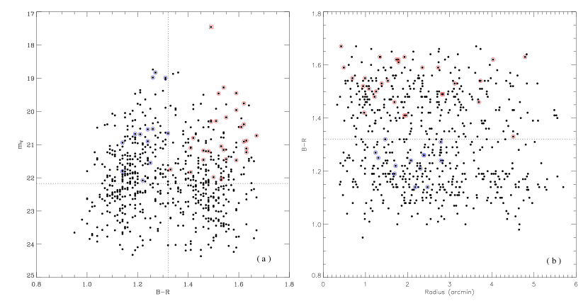
Figure 3: (a) Color-magnitude diagram of all GCs identified in S06. Improved photometry is obtained from Spitler, Forbes & Beasley (2008). GCs hosting a detected X-ray source are marked by an open circle. The vertical dashed line represents the division of blue ($B-R\leq 1.32$) and red ($B-R>1.3$) GCs, the horizontal line the turnover magnitude, following S06. Also plotted is the metal-rich UCD (Hau et al. 2009), with m_V=17.46, which is found to host an X-ray source and marked by a red square. (b) GC color vs. galactocentric radius.

Fig. 4 shows the F-band count rate and hardness ratio, defined as HR = (H2-M-S1)/(H2+M+S1), of the GC-LMXBs. Eleven sources have apparent luminosities above the Eddington luminosity for accreting neutron stars (NSs; $L_{\rm Edd}$$\sim$2$\times 10^{38}{\rm~{}ergs~{}s^{-1}}$). Among these, the four most luminous sources, with luminosities of $\sim$2-3 $L_{\rm Edd}$, are found in blue GCs. Each of these sources may be the superposition of several accreting NSs or an accreting black hole (BH), although theoretical considerations of dynamical processes in GCs predict the ejection of nearly all stellar-mass BHs on a short timescale of $\sim$$10^{8}{\rm~{}yr}$ (Kulkarni, Hut & McMillan 1993; Sigurdsson & Hernquist 1993). We note that the only accreting BH previously found in a GC is located in a blue GC in NGC 4472 (Maccarone et al. 2007). The GC probably lacks an intermediate-mass BH to dynamically eject stellar-mass BHs (Zepf et al. 2008). As Fig. 4a shows, bright Sombrero GCs (m${}_{\rm V}\leq$20) tend to host relatively bright LMXBs, whereas the LMXBs found in fainter GCs spread over the entire luminosity range ($\sim$$10^{37}-5\times 10^{38}{\rm~{}ergs~{}s^{-1}}$). In fact, the brightest LMXB is associated with one of the faintest GCs hosting an X-ray source. No significant trend is found in the X-ray flux-hardness ratio distribution of the GC-LMXBs (Fig. 4b). The brightest sources (those with luminosities above $\sim$$10^{38}{\rm~{}ergs~{}s^{-1}}$) show hardness ratios typical of accreting NSs (with photon-indices of $\sim$1.4-2). On the other hand, the fainter sources exhibit a variety of hardness ratios ranging from very soft ($\sim$-1.0) to very hard ($\sim$0.0). Analogous to a color-color diagram, Fig. 5 plots HR1 versus HR2 for the GC-LMXBs, where we define HR1 = (H1-S2-S1)/(H1+S2+S1) and HR2 = (H2-H1)/(H2+H1). Field X-ray sources (i.e., those not associated with GCs) detected within $R=4^{\prime}$ are also plotted for comparison. No distinct spectral behavior is evident between the blue and red GC-LMXBs, nor between the GC and field sources.

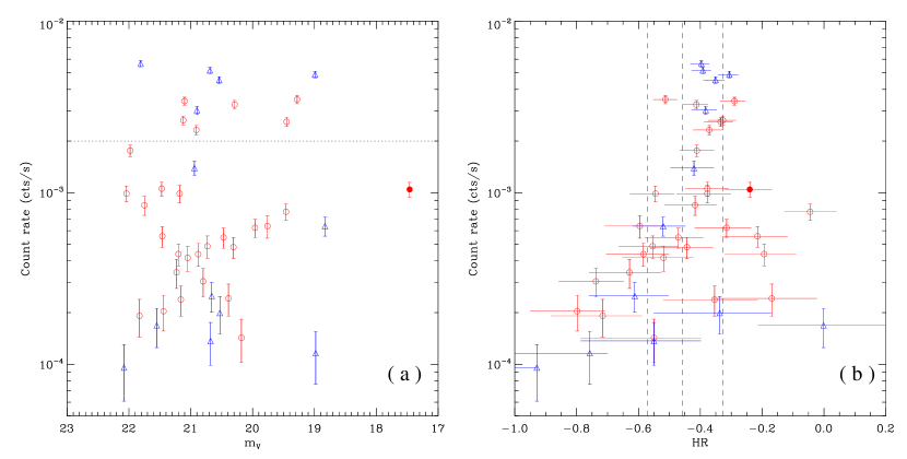
Figure 4: 0.4-6 keV count rate vs. (a) V-band magnitude and (b) hardness ratio, for the GC-LMXBs. The hardness ratio is defined as HR = (H2-M-S1)/(H2+M+S1). Blue and red GCs are plotted with blue triangles and red open circles, respectively. The UCD is plotted with a filled circle for comparison. The horizontal dashed line in (a) represents the Eddington luminosity of an accreting neutron star with a mass of 1.4 M_⊙. The vertical dashed lines in (b), from left to right, correspond to hardness ratios for an absorbed power-law spectrum with a fixed $N_{\rm H}=10^{21}{\rm~{}cm^{-2}}$ and a photon-index of 2.0, 1.7 and 1.4, respectively.

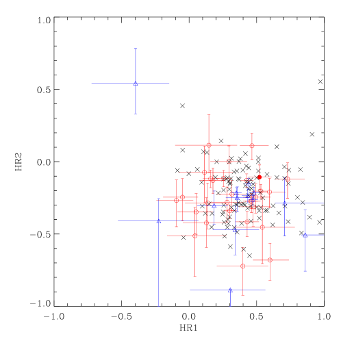
Figure 5: HR1 versus HR2, where HR1 = (H1-S2-S1)/(H1+S2+S1) and HR2 = (H2-H1)/(H2+H1). The blue and red symbols are the same representation of GC-LMXBs as in Fig. 4a., whereas black crosses represent those field X-ray sources detected within $R=4^{\prime}$ and simultaneously detected in the F-, M- and H2-bands. For clarity, error bars are not shown for the field sources, which have a similar uncertainty range as those of the GC-LMXBs.

We also note that an ultra-compact dwarf (UCD) associated with Sombrero was identified in the HST/ACS images (Hau et al. 2009), which in many aspects appears as a “giant version” of a GC. We confirm the positional coincidence between the UCD and an X-ray source (source 275 in Table 1). The centroids of the two objects are separated by $0\farcs 4\pm 0\farcs 4$, a value comparable with the optical half-light radius ($\sim$0$\farcs$33) of the UCD. We show this pair of sources in Fig. 4 and Fig. 5 in comparison with the GC-LMXBs. The UCD has a 0.5-8 keV luminosity of $\sim$$10^{38}{\rm~{}ergs~{}s^{-1}}$ and a relatively soft spectrum (showing HR $\approx$ -0.25) compared to most of the GC-LMXBs.

3.2 Spatial properties

The spatial distribution of detected X-ray sources shows a clear concentration within the optical extent of the galaxy (Fig. 1b, c). The well known presence of a prominent dust lane and its association with radio continuum emission (Bajaja et al. 1988) and H$\alpha$ emission (Li et al. 2007) indicate star-forming activities in the disk. Both the radio continuum and H$\alpha$ fluxes suggest a rather low star formation rate of 0.1-0.2 M_⊙/yr, which in turn predicts $\leq$4 high-mass X-ray binaries (HMXBs) with luminosities $\geq 10^{37}{\rm~{}ergs~{}s^{-1}}$ (Grimm, Gilfanov & Sunyaev 2003). Hence the bulk of sources associated with the galaxy are presumably LMXBs. We further note that two sources are only detected in the S-band (sources 159 and 189 in Table 1), suggesting that they are super-soft sources (SSS; e.g., Di Stefano & Kong 2004). As SSSs are thought be a different population than LMXBs, we do not include these two sources in the following analysis.

Fig. 6a shows the azimuthally-averaged radial distribution of the source surface density. The GC-LMXBs cover a radial range between 0$\farcm$4-4$\farcm$8, over which they appear more concentrated than the entire GC population. This concentration is likely attributed to those sources associated with red GCs (Fig. 3) which have a steeper radial distribution than the blue GCs. The field sources presumably consist of two components: LMXBs predominantly present in the bulge, and cosmic AGNs dominating the surface density at large radii. Indeed, the 2MASS K-band starlight (Jarrett et al. 2003), when scaled by a factor of 8.1 X-ray sources per $10^{10}L_{\odot,K}$ as derived for nearby galactic bulges (Gilfanov 2004), is a reasonable characterization of the surface density distribution of the field sources within $R\sim$2^′ (roughly twice the K-band effective radius of the galaxy), as expected if the field LMXBs are distributed following the old stellar populations.

However, at radii outside the optical extent of the galaxy ($R\gtrsim$4^′), deviations in the number of field sources from the expected cosmic contribution are significant. The cosmic contribution at a given position across the FoV can be determined from the Log$N$-Log$S$ relation of cosmic AGNs (Moretti et al. 2003), accounting for the local detection threshold (Fig. 2). Specifically, the detection threshold in terms of F-band count rate is converted into a 0.5-2 keV flux, as adopted by Moretti et al. (2003; Eqn. 2 therein), assuming an intrinsic power-law spectrum with a photon index of 1.4, suitable for cosmic AGNs (Moretti et al. 2003), and the Galactic foreground absorption. This cosmic component is shown by a dashed curve in Fig. 6a. Between $R=$4^′-9^′, the expected number of cosmic AGNs is 52.3, while the observed number of field sources is 101. Only at radii beyond 9^′ do the observed and predicted surface density distributions agree with each other (19.2 versus 21; Fig. 6a). While the adopted Log$N$-Log$S$ relation is derived from a combination of shallow wide-field and deep pencil-beam surveys (Moretti et al. 2003), the surface density of cosmic AGNs is expected to vary from field to field. The normalized cosmic variance can be estimated as (e.g., Lahav & Saslaw 1992)

$$\sigma^{2}_{c}=\frac{1}{\Omega^{2}}\int w(\theta){d\Omega_{1}}{d\Omega_{2}}=C_{\gamma}\theta^{\gamma-1}_{0}\Theta^{1-\gamma},$$ (1)

where $w(\theta)=(\theta/\theta_{0})^{1-\gamma}$ is a power-law angular correlation function (Peebles 1980), $\theta_{0}$ the correlation length, $C_{\gamma}$ a numerical factor dependent on the index $\gamma$, and $\Omega=\Theta^{2}~{}deg^{2}$ the size of the FoV. For the canonical value of $\gamma=1.8$ we have $C_{\gamma}\approx 2.25$, and we adopt $\theta_{0}\approx 0.00214~{}deg$ (i.e., 7$\farcs$7) measured from a serendipitous XMM-Newton survey reaching a flux limit of $F_{0.5-2{\rm~{}keV}}\sim 10^{-15}{\rm~{}ergs~{}s^{-1}~{}cm^{-2}}$ (Ebrero et al. 2009), comparable to the flux limit achieved in the Sombrero field. Hence the fractional cosmic variance is $\sigma_{c}\approx 0.16$ for the $4^{\prime}-9^{\prime}$ annulus in which the source overdensity is found. Combining the cosmic and Poisson variances ($\sigma=\sqrt{\sigma_{c}^{2}+\sigma_{P}^{2}}\approx 0.21$), the significance of the overdensity is $\sim$4.4 $\sigma$. Unidentified Galactic interlopers may contribute to the overdensity, but this is unlikely given the relatively high Galactic latitude of Sombrero. On the other hand, a small fraction of the identified interlopers can in fact be background galaxies or AGNs. The removal of such sources has the effect of reducing the local cosmic background, and hence the actual overdensity is likely more significant than estimated here. Neither can the overdensity be accounted for by simply increasing the normalization of the galactic bulge component, as the K-band surface brightness drops steeply with radius and becomes negligible beyond $\sim$$4^{\prime}$. We discuss in § 4 the possibility that the overdensity originates from sources physically associated with the halo of Sombrero.

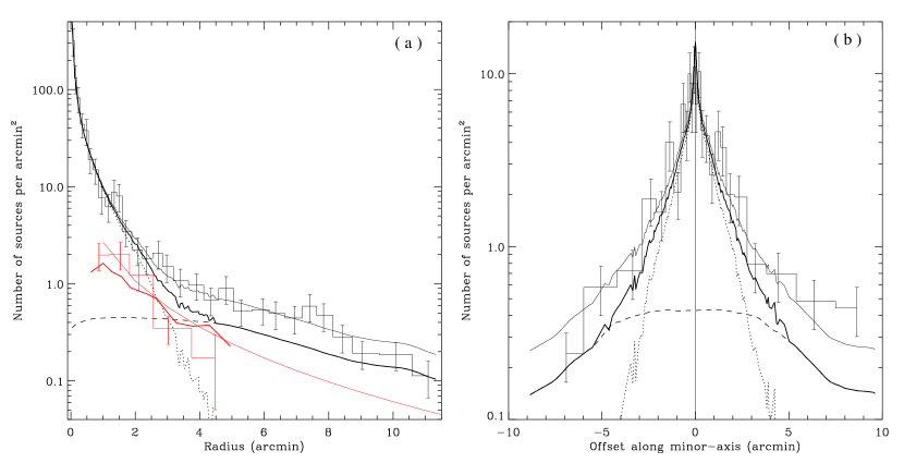
Figure 6: (a) Radial surface density distributions of different classes of sources. The histograms (Black: field sources; red: GC-LMXBs) are adaptively grouped to have a minimum of 10 sources per bin. The thick black solid curve represents a characterization of the field source distribution, which consists of contributions of field LMXBs (dotted curve; a normalized 2MASS K-band light radial profile) and a cosmic background of AGNs (dashed curve). The normalizations of the LMXB and AGN components are adopted from Gilfanov (2004) and Moretti et al. (2003), respectively. The thin black solid curve consists of the same LMXB contribution, but with 1.8 times higher contribution from the AGNs. The thick and thin curves in red represent the distribution of the S06 GCs and a de Vaucouleurs law characterizing the GC distribution derived by Rhode & Zepf (2004), both multiplied by a factor of 0.06. (b) Similar to (a), but for the vertical surface density distribution of field sources along the galaxy’s minor-axis. The source density is averaged within parallel slices of 10 arcmin in width. North is positive.

3.3 Number-flux relation

We construct differential number-flux relations (NFRs; Fig. 7) for the field sources detected in the two annuli with inner-to-outer radii of 10^′′-4^′ (hereafter A1) and 4^′-9^′ (hereafter A2) and for the GC-LMXBs. The inner radius of A1 is chosen to minimize the uncertainty due to source confusion in the innermost regions. We also exclude a region approximately coincident with the dust lane (enclosed by the dashed ellipses in Fig. 1), where both HMXBs and additional interstellar absorption are likely present. Moreover, we consider only sources detected in the F-band for NFR A1 and only sources detected in the M-band (0.7-2 keV) for NFR A2. The latter, in particular, ensures an optimal comparison with the 0.5-2 keV Log$N$-Log$S$ relation of Moretti et al. (2003). A1 and A2 contain 159 and 93 sources, respectively. As the characteristic spectra of LMXBs and cosmic AGNs are not identical, we choose to refer “flux” to the observed count rate, instead of a converted incident flux.

Our analysis of the NFRs follows the procedure described in Wang (2004), accounting for the dependence of the detection completeness on the local PSF, effective exposure and background, as well as the so-called X-ray Eddington bias that describes the probability distribution of observed count rates due to the Poisson uncertainties and the intrinsic slope of the NFR. The 90% completeness limit is estimated to be $\sim$$2\times 10^{37}{\rm~{}ergs~{}s^{-1}}$ for sources detected in A1 and the GC-LMXBs, while this limit is significantly higher in A2 ($\sim$$6\times 10^{37}{\rm~{}ergs~{}s^{-1}}$). As sources in A1 are dominated by the galactic old stellar populations, we use the K-band starlight distribution as a spatial weight to calculate the accumulated functions of the incompleteness and Eddington bias for these galactic sources, whereas the intrinsic distribution of the cosmic AGNs is assumed to be uniform across the field. While approximately half of the sources in A2 are possibly associated with Sombrero (§ 3.2), we also assume a uniform spatial distribution for these sources, for simplicity.

As for the radial surface density distributions (§ 3.2), we fit NFR A1 with two components: a cosmic component, assuming the Log$N$-Log$S$ relation of Moretti et al. (2003), and a galactic component. The cosmic component contributes $\sim$10% to the NFR. We begin with a power-law model for the galactic component,

$$\left({dN\over dS}\right)=KS^{-\alpha},$$ (2)

where $S$ is in units of ${\rm cts~{}s^{-1}}$. The fit gives $\alpha=1.59^{+0.08}_{-0.08}$ and $K=0.44^{+0.37}_{-0.20}$ sources per ${\rm cts~{}s^{-1}}$. With C-statistic/d.o.f. = 22.1/17, this fit is only acceptable at a confidence level of 29%. A broken power-law (Fig. 7) gives a much improved fit with C-statistic/d.o.f. = 11.4/15, acceptable at a confidence level of 91%. The fitted power-law indices are $1.23^{+0.13}_{-0.14}$ and $2.43^{+0.31}_{-0.27}$ below and above the break of $1.05^{+0.42}_{-0.24}\times 10^{-3}{\rm~{}counts~{}s^{-1}}$, which corresponds to a 0.5-8 keV intrinsic luminosity of $1.0\times 10^{38}{\rm~{}ergs~{}s^{-1}}$. The change in the slope is of $\sim$ 4$\sigma$ significance; the fitted indices are consistent with those derived from deep Chandra observations of three elliptical galaxies NGC 3379, NGC 4278 and NGC 4697 (Kim et al. 2009). The break luminosity, on the other hand, is marginally higher than that found in the elliptical galaxies ($\sim$$6\times 10^{37}{\rm~{}ergs~{}s^{-1}}$).

For the NFR of GC-LMXBs, we consider only the galactic component, for which a power-law model, with an index of $1.13^{+0.14}_{-0.14}$ and C-statistic/d.o.f. = 1.2/5, provides an acceptable fit at a confidence level of 99%. Due to the limited number statistics, there is no obvious need for a broken power-law model to characterize this NFR. Finally, we find that the Log$N$-Log$S$ relation of Moretti et al. (2003) is inconsistent with the NFR A2 (C-statistic/d.o.f. = 46.7/9), in particular falling short at M-band count rates below $9\times 10^{-4}{\rm~{}cts~{}s^{-1}}$ (Fig. 7). Instead, the NFR A2 can be well fitted by a power-law model with a slope of $2.03^{+0.12}_{-0.12}$, significantly steeper than Moretti et al.’s slope of $\sim$1.60 over the considered flux range. The removal of background interlopers (§ 3.3) may steepen the NFR A2 at the bright end. To account for this effect, we reconstruct the NFR A2 without removing any identified interlopers. This new NFR can be fitted by a power-law with a slope of $1.89^{+0.12}_{-0.12}$. This again suggests that sources detected in A2 originate in part from a population distinct from cosmic AGNs.

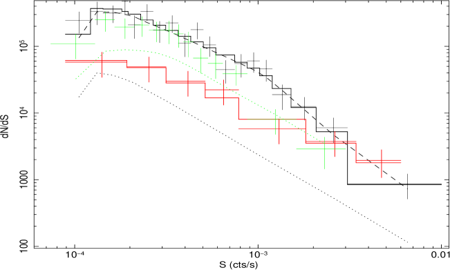
Figure 7: Differential number-flux relation of field sources detected between 0$\farcm$1-4^′ (A1; black) and 4^′-9^′ (A2; green), and sources associated with GCs (red). The count rates are measured in the F-band (0.4-6 keV) for A1 sources and GC-LMXBs and in the M-band (0.7-2 keV) for A2 sources. Data points are adaptively grouped to have a minimum of 6 sources per bin. The black histogram represents an acceptable fit to the A1 NFR, consisting with a broken power-law for the galactic component (dashed curve) and a cosmic component from Moretti et al. (dotted curve). The red histogram represents an acceptable power-law fit to the GC NFR. The green dotted curve represents the expected cosmic component in the A2 NFR. Note the turnover of the NFRs and models at low count rates, which results from the incompleteness and Eddington bias in the source detection.

3.4 Unresolved X-ray emission from GCs

While 41 GC-LMXBs are found (§ 3.1), the rest (93.8%) of the S06 GCs remain undetected in X-rays. Nevertheless, some X-ray emission is expected to come from these GCs. For instance, some GCs may host an LMXB that is fainter than the local detection threshold ($\sim$$10^{37}{\rm~{}ergs~{}s^{-1}}$). The “X-ray emission” from the undetected GCs can be quantified through a fluctuation analysis (e.g., Miyaji & Griffiths 2002; Hickox & Markevitch 2007; Hickox et al. 2009) and subsequently provides useful constraints on the GC-LMXB population, such as the shape of the NFR at fluxes significantly below the detection threshold. The procedure is as follows. First, we collect 0.4-6 keV source counts registered within the 90% EER (ranging from 1$\farcs$5-5$\farcs$5) around individual undetected GCs. To minimize contamination from nearby X-ray sources, a GC is excluded if it is located within three times the 90% EER of a detected X-ray source. This results in a total of 483 GCs, the source counts of which range from 0 to 18 cts. The number distribution of source counts is plotted in Fig. 8a. showing a bump representing the statistical fluctuation of the local background and a high-count tail presumably arising from the collective emission from the GCs. For comparison, we also show the mean number distribution of counts collected in a similar way from “empty” regions (histogram in Fig. 8a), i.e, positions $\pm 5^{\prime\prime}$ in R.A. and Dec. from the GC centroids. The distribution of counts collected from the GCs shows a clear excess above 5 cts. Corrected for the mean exposure at the GC positions, this excess corresponds to an integrated net count rate of $(2.1\pm 0.1)\times 10^{-3}{\rm~{}cts~{}s^{-1}}$, or 7.4 $\sigma$ over the local background. Repeating this exercise on a subset of the GCs, we estimate an integrated net count rate of $(7.5\pm 0.7)\times 10^{-4}{\rm~{}cts~{}s^{-1}}$ for 101 red GCs brighter than the turnover magnitude, $(5.3\pm 0.6)\times 10^{-4}{\rm~{}cts~{}s^{-1}}$ for 149 blue GCs brighter than the turnover magnitude, $(6.9\pm 0.7)\times 10^{-4}{\rm~{}cts~{}s^{-1}}$ for 116 red GCs are fainter than the turnover magnitude, $(1.1\pm 0.3)\times 10^{-4}{\rm~{}cts~{}s^{-1}}$ for 117 blue GCs are fainter than the turnover magnitude, respectively. The red GCs apparently also show a higher integrated unresolved X-ray flux than the blue GCs.

Second, we statistically constrain the net contribution from the undetected GCs, and moreover, their NFR at low fluxes, in the following steps.

i) The shape of the NFR is assumed to be a broken power-law:

$$\frac{dN_{\rm GC}}{dS}=\left\{\begin{array}[]{l@{\quad\quad}l}KS^{-\alpha_{1}}&(S_{\rm min}\leq S<S_{\rm b}),\\ KS_{\rm b}^{\alpha_{2}-\alpha_{1}}S^{-\alpha_{2}}&(S_{\rm b}\leq S),\\ \end{array}\right.$$ (5)

where $S_{\rm min}=10^{-6}{\rm~{}cts~{}s^{-1}}$ is the minimum flux above which the NFR is evaluated. This value corresponds to a luminosity of $\sim$$10^{35}{\rm~{}ergs~{}s^{-1}}$, reasonable for LMXBs. We note that a fluctuation analysis is typically sensitive to 1 $\sigma$ below the mean background ($\sim$2 cts here), which is $\sim$0.6 cts, corresponding to a count rate of $\sim$3$\times 10^{-6}{\rm~{}cts~{}s^{-1}}$. We fix the bright-end index, $\alpha_{2}$, at the value of 1.13, justified by the goodness of the power-law characterization for the identified GC-LMXBs in § 3.3. The normalization $K$ is effectively determined by the total number of detected GC-LMXBs with count rates above the 100% completeness limit of $3\times 10^{-4}{\rm~{}cts~{}s^{-1}}$ (28 of 659 GCs). Therefore the free parameters are the faint-end index, $\alpha_{1}$, and the break flux, $Sb$, which is assumed to be no higher than $3\times 10^{-4}{\rm~{}cts~{}s^{-1}}$.

ii) With Monte Carlo simulations, we generate source counts from the 483 undetected GCs, based on the above NFR. The expected source count of a GC is the sum of the local background flux (which has been determined in the source detection procedure) and the NFR-predicted flux, multiplied by the local effective exposure and then Poisson-randomized. In each simulation run, a distribution of $N_{{\rm sim},i}$, the number of GCs with $i$ counts, is generated. The deviation between the simulated and observed distribution (Fig. 8) is evaluated by the modified C-statistics (Cash 1979),

$$C=2\sum_{i}[N_{{\rm sim},i}-N_{{\rm obs},i}+N_{{\rm obs},i}({\rm ln}N_{{\rm sim},i}-{\rm ln}N_{{\rm obs},i})].$$ (6)

iii) For a given pair of $\alpha_{1}$ and $S_{b}$, 1000 simulations are run and the mean value of $C$ is calculated. A best-fit is found at the minimum of $C/d.o.f.$=7.22/10, which is acceptable at a confidence level of 97%. The fit is not sensitive to $S_{b}$, but gives $\alpha_{1}=1.55^{+0.15}_{-0.15}$ (Fig. 8b). Comparing with the bright-end index $\alpha_{2}=1.13^{+0.14}_{-0.14}$, this rules out a flattened NFR toward fainter fluxes at a 2 $\sigma$ significance. The corresponding mean value of $N_{{\rm obs},i}$ is shown in Fig. 8a.

iv) The above procedure has two implicit assumptions: (1) the source counts from individual GCs are independent, and (2) the GC X-ray flux is not dependent on other GC properties. While the first assumption is generally true given the small sky area occupied by the GCs, the second assumption is inconsistent with the trend that more luminous and denser GCs have a larger chance to host an LMXB. To test this effect, we repeat our procedure for those GCs above the turn-over magnitude, so that the dependency on GC properties is minimized, but this comes at the price of reduced statistics. The corresponding best-fit $\alpha_{1}$ is $1.42^{+0.26}_{-0.19}$, again implying that the NFR does not flatten toward fainter fluxes.

v) Stellar populations other than LMXBs, such as cataclysmic variables (CVs) and millisecond pulsars, can also contribute to the detected X-ray counts in individual GCs. The collective luminosity of such populations correlates with GC mass, and is expected to be $\lesssim 10^{35}{\rm~{}ergs~{}s^{-1}}$ per GC. To evaluate the effect of such a contribution, we simply add a delta function at $10^{-6}{\rm~{}cts~{}s^{-1}}$ to the NFR model and repeat the simulations. This results in a best-fit $\alpha_{1}$=$1.40^{+0.20}_{-0.16}$, again showing no evidence of a flattened NFR at faint fluxes.

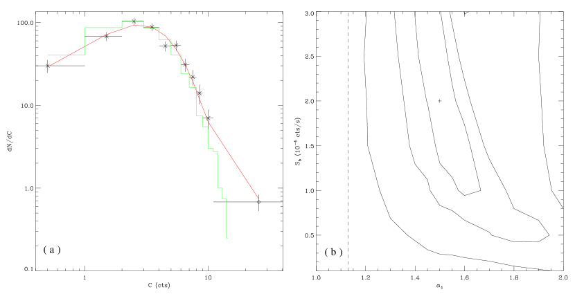
Figure 8: (a) Number distribution of source counts for the GCs: crosses: X-ray-undetected GCs; diamond: X-ray-detected GCs with fluxes below the detection completeness limit. The histogram is a representation of the number distribution of local background counts. The curve shows the predicted number distribution from the best-fit model NFR. See text for details. (b) The 68%, 90% and 99% confidence contours of the faint-end index and the break flux. The plus sign marks the best-fit values. The vertical dash line marks the best-fit value of the bright-end index derived from the X-ray-detected GCs.

3.5 Variability

Transients and variable X-ray sources are often found in early-type galaxies. Here we quantify the variability of the GC-LMXBs and the field sources detected within $R=4^{\prime}$, where the FoV is common to all three observations. The net count rate of each source in each of the three observations is determined in a homogeneous way, similar to the determination of the average source count rate from the combined data. If a source is below the detection threshold in a given observation, its net count rate is measured in the same way as described in § 3.4. We define source variability $V=F_{\rm h}/F_{l}$, where $F_{\rm h}$ is the highest detected count rate among individual detections, and $F_{\rm l}$ the statistical upper limit of the lowest detected count rate. The variability is plotted versus the average count rate (Fig. 9a) and the hardness ratio of individual sources (Fig. 9b). $\sim$44% (83 of 188) of the field sources and $\sim$36% (15 of 41) of the GC-LMXBs exhibit $V>2$. $\sim$13% (24 of 188) of the field sources are strongly variable (defined as $V>10$), whereas this number is $\sim$7% (3 of 41) in GC-LMXBs. Two red and one blue GC-LMXBs are detected in only one observation, but none of them has $V>10$. We also find that 53 of the field sources are detected in only one observation, and thus may be transient sources. 17 of these 53 sources, or $\sim$9% of the total field sources considered, exhibit $V>10$ and hence are the most probable transients. For comparison, five and three transients, also defined as $V>10$, are found among $\sim$100 source detected in NGC3379 and $\sim$180 sources in NGC4278, respectively (Brassington et al. 2008, 2009). In another elliptical galaxy, NGC 4636, which is comparable to Sombrero in stellar mass but more massive than NGC3379 and NGC4278, two such transient candidates are found among $\sim$230 detected sources (J. Posson-Brown, private communication).

The two most variable sources (with $V>600$) exhibit a super-Eddington luminosity for an NS, as well as a hardness ratio softer than typical NSs, implying that they are likely accreting BHs. A close examination of the data reveals that the brighter one of these two sources, centered at [R.A.,DEC.]=[12:40:01.85, -11:36:15.3], is only visible in Obsid. 9532, and the fainter one, centered at [R.A.,DEC.]=[12:40:00.95, -11:36:54.1], only appears in Obsid. 1586. On the other hand, the super-Eddington GC-LMXBs show no significant variability, suggesting that they are superpositions of accreting objects, most likely NSs.

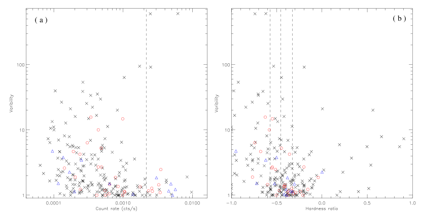
Figure 9: Source variability (see text for definition) vs. (a) count rate and (b) hardness ratio. Field sources detected within $R=4^{\prime}$ are shown by crosses, while LMXBs detected in blue and red GCs are shown by blue triangles and red circles, respectively. The dashed line in (a) represents the Eddington luminosity of an accreting NS with a mass of 1.4 M_⊙. The dashed lines in (b), from left to right, correspond to hardness ratios of an absorbed power-law spectrum with a fixed $N_{\rm H}=10^{21}{\rm~{}cm^{-2}}$ and a photon index of 2.0, 1.7 and 1.4, respectively.

4 Discussion

4.1 LMXB luminosity function

In § 3.4 we quantify the collective X-ray emission from GCs below the X-ray detection threshold. In particular, the number-flux relation of these sources is examined. Hereafter we use the term “luminosity function” (LF) for formality. Our fluctuation analysis rules out a slope of the LF flatter than 1.1 below $10^{37}{\rm~{}ergs~{}s^{-1}}$ at 2 $\sigma$ significance. In fact, the inferred faint-end power-law index is steeper than that of the bright-end. This is contrary to the findings in recent X-ray studies of GC populations in several elliptical galaxies, including NGC 3379, NGC 4278, NGC 4697 (Kim et al. 2009) and NGC 5128 (Voss et al. 2009), and in the bulge of M31 (Voss & Gilfanov 2007), in which deep Chandra observations allow for detection of faint GC-LMXBs down to $10^{36}-10^{37}{\rm~{}ergs~{}s^{-1}}$. In these galaxies the GC LF appears flattened at the faint-end with respect to its slope at the bright-end.

The LF of field LMXBs determined in § 3.3, on the other hand, is consistent with previous studies in which a single power-law index of $\sim$1.8 is typically found. We can also examine its behavior below our detection limit, utilizing the unresolved X-ray emission. In particular, the 2-6 keV unresolved emission is thought to almost entirely originate from stellar populations consisting of faint, unresolved LMXBs and even fainter stellar objects, such as coronally active binaries (ABs) and CVs (Sazonov et al. 2006; Revnivtsev et al. 2006, 2007, 2008). Fig. 10 shows the azimuthally-averaged radial intensity distribution of the 2-6 keV unresolved emission (crosses), after removal of all detected sources with F-band count rates above the completeness limit of $3\times 10^{-4}{\rm~{}cts~{}s^{-1}}$. Our source-removal procedure effectively excludes $\sim$96% of the source photons. The 4% PSF-scattered photons can be accounted for by following the radial distribution of detected bright sources. This PSF-scattered component is shown in Fig. 10 by a dotted curve. In bulges and elliptical galaxies, the collective 2-6 keV emissivity (per stellar mass) of CV+AB is likely universal and has been calibrated to better than $\sim$15% (Revnivtsev et al. 2008). The CV+AB contribution for Sombrero is shown in Fig. 10 by a normalized K-band radial intensity distribution (dashed curve). The contribution of faint LMXBs to the 2-6 keV unresolved emission is then determined by extrapolating a given LF. We test different values of the index $\alpha$ for LMXBs toward the faint-end, fixing the bright-end index at 1.6 (§ 3.3) and the break luminosity at the completeness limit. The sum of PSF+(CV+AB)+LMXB is shown by solid curves in Fig. 10 for representative values of $\alpha$=1.6 (no flattening) and $\alpha$=1.0. Clearly the observed unresolved emission indicates a flattened LF for the field LMXBs below $\sim$$3\times 10^{37}{\rm~{}ergs~{}s^{-1}}$.

Figure 10: Background-subtracted, exposure-corrected radial intensity distributions of the unresolved 2-6 keV emission, shown by crosses. The estimated contribution to the unresolved emission from PSF scattering of detected sources (dotted curve) and CV+AB (dashed curve) are marked. The two solid curves represent the sum of PSF+CV+AB+LMXB (unresolved), the latter estimated by assuming assuming a LMXB LF, the faint-end power-law index of which is either 1.0 or 1.6. See text for details.

4.2 Origin of the source overdensity

In § 3.2 we show an excess of X-ray sources detected at large galactocentric radii with respect to the expected number and typical spatial variance of cosmic AGNs. These sources are plausibly associated with Sombrero. Here we discuss their possible parent population.

In light of the presence of a large GC population in Sombrero to a galactocentric radius of $\sim$50 kpc (Rhode & Zepf 2004), a possible host of these X-ray sources is GCs located at large radii. Based on ground-based observations, Rhode & Zepf (2004) reported a total of $\sim$1900 GC candidates, whose surface density distribution is well characterized by a de Vaucouleurs law with an effective radius of $\sim$6$\farcm$2, as shown in Fig. 6. This surface density distribution predicts that $\sim$22% of the whole GC population is located between $R=$4^′-9^′, where the X-ray source overdensity is found. Assuming that 6% of these GCs host a detectable X-ray source, a value appropriate for the S06 GCs, 32.5 GC-LMXBs are expected, which is marginally sufficient to account for the observed overdensity. However, it is premature to claim that GCs are the primary host of the observed overdensity, for the following reasons: 1) while there are 96 S06 GCs identified at $R\geq 4^{\prime}$, only 3 of them ($\sim$3%) are found to be associated with an X-ray source. The higher percentage (6%) of associations for the entire S06 GCs presumably arises from associations with red GCs which have a steeper concentration in the bulge than the blue ones; 2) at large radii, contamination of interlopers becomes increasingly significant for the Rhode & Zepf GC candidates and the true GC population may have a steeper surface density distribution. Indeed, in a spectroscopic follow-up study, Bridges et al. (2007) found a substantial fraction of the Rhode & Zepf GC candidates to be interlopers; 3) The same GC distribution of Rhode & Zepf also predicts $\lesssim$9.8 X-ray sources detectable (with a detection threshold of $5\times 10^{-4}{\rm~{}cts~{}s^{-1}}$, or $\sim$$5\times 10^{37}{\rm~{}ergs~{}s^{-1}}$) at $R=9^{\prime}$-11$\farcm$5, or a mean surface density of $\lesssim$0.06 source per arcmin² over the cosmic component, which is not observed. The Rhode & Zepf (2004) GCs, whose sky positions are unpublished, could be useful to directly test this possibility.

Another possibility is binary systems, favorably containing an accreting NS, which are ejected from the inner galactic regions due to the recoil of the system after the supernova that created the NS. In Fig. 6b the surface density distribution of field sources along the minor-axis of the disk is shown. Compared to the starlight distribution (dotted curve in Fig. 6b), the detected sources show a clear overdensity as close as 1 arcmin from the midplane. This is reminiscent of a distribution of sources ejected from the disk. The spatial distribution of Galactic NSs resulting from supernova kicks has long been the subject of studies, e.g., by Paczy$\acute{n}$ski (1990), among others. Recently, Zuo, Li & Liu (2008) modelled the spatial distribution of Galactic X-ray binaries, accounting for the kinematic evolution of the kicked binary systems. However to our knowledge, a similar study in the scope of galactic spheroids (i.e., bulges of early-type spirals and elliptical galaxies) has not been carried out.

A third and perhaps more controversial possibility is X-ray binaries formed in relaxed remnants of recent mergers, which are now falling back to the inner galactic regions, as suggested by Zezas et al. (2003) for the field sources detected in two elliptical galaxies, NGC4261 and NGC4697. These sources show an azimuthally non-uniform distribution toward large radii. We have examined the azimuthal distribution of the sources detected with $R=$4^′-9^′, but found no significant non-uniformity.

It is conceivable that a similar source overdensity also exists in typically massive elliptical galaxies. We search the Chandra archival data for suitable galaxies to test this possibility. Four elliptical galaxies are thus selected, including NGC 3379, NGC 4365, NGC 4636 and NGC 4697. The distances (10-20 Mpc) and cumulative Chandra exposure ($\sim$200 ks) of these galaxies allow for a similar source detection threshold and a similar coverage of radial extent as we achieved for Sombrero. Indeed, the discrete source populations in each of these galaxies have been the subject of recent studies (Brassington et al. 2008; Sivakoff et al. in preparation; Posson-Brown et al. 2009; Sivakoff et al. 2008). Here we perform source detection and construct a radial source density profile for each galaxy (Fig. 11), in the same way as for Sombrero, except that no GC-LMXBs are identified due to the lack of a published GC catalogue for any of these galaxies. As shown in Fig. 11, the surface density profiles of NGC 3379 and NGC 4697 can be described by a galactic component following the K-band starlight and a cosmic component, whereas the other two galaxies, NGC 4365 and NGC 4636, exhibit a source overdensity above the expected cosmic contribution in regions beyond their half-light radii. NGC 4365 and NGC 4636 are two massive Virgo ellipticals, with a total stellar mass even higher than that of Sombrero, whereas NGC 3379 and NGC 4697 are each about 3 times less massive than Sombrero. We emphasize, however, that unidentified GC-LMXBs must contribute to part, if not all, of the observed overdensity in NGC 4365, NGC 4636 and Sombrero.

Figure 11: Radial surface density distributions for sources detected in (a) NGC 3379, (b) NGC 4365, (c) NGC 4636 and (d) NGC4697. The curves have the same representation as in Fig. 6.

5 Summary

Our study of the X-ray sources in the Sombrero galaxy can be summarized as follows:

1. With a detection limit of $10^{37}{\rm~{}ergs~{}s^{-1}}$, a total of 383 sources are detected within a projected galactocentric radius of $R$=11$\farcm$5. Among them, 41 sources, presumably LMXBs, are found to be associated with GC candidates identified through HST observations covering the optical extent of Sombrero ($R\sim$4). 28 of the 41 sources are found in metal-rich GCs, indicating that metal-rich GCs have a higher probability of hosting an LMXB. On the other hand, metal-poor GCs host the four brightest GC-LMXBs whose individual luminosities exceed the Eddington luminosity of an accreting NS.

2. The differential number-flux relation (i.e., luminosity function) of the detected GC and field sources are quantified by a power-law model. The slopes are $\sim$1.1 and $\sim$1.6 for the GC and field sources, respectively, consistent with previous findings in nearby elliptical galaxies.

3. Photon counts from the positions of X-ray-undetected GCs show a $\sim$7.4 $\sigma$ excess above the local background. Based on these counts, a fluctuation analysis shows that the differential number-flux relation does not flatten at fluxes below $\sim$$10^{37}{\rm~{}ergs~{}s^{-1}}$, contrary to recent findings in several elliptical galaxies and the bulge of M31.

4. For field sources, the 2-6 keV unresolved emission places a tight constraint on the differential number-flux relation, implying a flattened slope of $\sim$1.0 below $\sim$$10^{37}{\rm~{}ergs~{}s^{-1}}$.

5. A total of 101 sources are detected in the halo of Sombrero. This is a $\sim$4.4 $\sigma$ excess above the expected number of cosmic AGNs, indicating that either the cosmic background is unusually high in this direction or about half of these sources are associated with Sombrero.

We are grateful to Ryan Hickox for his advice on the fluctuation analysis. This work is supported by the SAO grant G08-9088.

Table 1: Chandra Source List

Source	CXOU Name	$\delta_{x}$ (′′)	CR	CR1	CR2	CR3	CR4	HR	HR1	HR2	Flag
(1)	(2)	(3)	(4)	(5)	(6)	(7)	(8)	(9)	(10)	(11)	(12)
1	J123919.62-113214.9	1.0	$1.76\pm 0.24$	$-0.07\pm 0.07$	$0.34\pm 0.12$	$0.94\pm 0.15$	$0.55\pm 0.14$	$-0.38\pm-0.01$	$0.55\pm 0.01$	$-0.26\pm-0.01$	B, M, H2
2	J123920.06-113628.5	1.4	$0.60\pm 0.17$	$0.18\pm 0.11$	$0.12\pm 0.06$	$0.26\pm 0.08$	$0.04\pm 0.07$	$-0.88\pm-0.04$	$-0.10\pm-0.03$	$-0.76\pm-0.09$	B, M
3	J123920.46-113258.5	2.1	$0.31\pm 0.13$	$-0.07\pm 0.00$	$0.05\pm 0.06$	$0.36\pm 0.10$	$-0.03\pm 0.07$	$-0.96\pm-0.02$	$0.96\pm 0.02$	$-0.96\pm-0.02$	M
4	J123920.59-113915.6	1.2	$0.58\pm 0.15$	$-0.02\pm 0.06$	$0.03\pm 0.04$	$0.50\pm 0.11$	$0.08\pm 0.07$	$-0.72\pm-0.01$	$0.97\pm 0.01$	$-0.72\pm-0.01$	B, M
5	J123920.69-113408.1	1.3	$0.81\pm 0.17$	$-0.01\pm 0.06$	$0.18\pm 0.08$	$0.42\pm 0.10$	$0.22\pm 0.09$	$-0.46\pm-0.01$	$0.45\pm 0.01$	$-0.32\pm-0.02$	B, M
6	J123923.66-113819.8	1.5	$0.37\pm 0.12$	$0.02\pm 0.05$	$0.12\pm 0.06$	$0.16\pm 0.07$	$0.06\pm 0.06$	$-0.68\pm-0.02$	$0.05\pm-0.03$	$-0.48\pm-0.04$	M
7	J123924.19-113838.0	0.9	$0.67\pm 0.14$	$0.07\pm 0.08$	$0.00\pm 0.03$	$0.31\pm 0.08$	$0.29\pm 0.08$	$-0.14\pm-0.01$	$0.61\pm 0.03$	$-0.04\pm-0.02$	B, M, H2
8	J123925.15-113836.9	1.1	$0.40\pm 0.11$	$-0.04\pm 0.00$	$0.00\pm 0.03$	$0.35\pm 0.09$	$0.09\pm 0.06$	$-0.55\pm-0.02$	$0.97\pm 0.02$	$-0.58\pm-0.02$	B, M
9	J123925.23-113408.8	1.4	$0.67\pm 0.19$	$0.10\pm 0.11$	$0.14\pm 0.08$	$0.44\pm 0.11$	$-0.01\pm 0.07$	$-0.97\pm-0.01$	$0.30\pm 0.02$	$-0.96\pm-0.02$	B, M
10	J123926.66-113250.0	1.9	$0.44\pm 0.20$	$0.24\pm 0.15$	$0.07\pm 0.06$	$0.27\pm 0.09$	$-0.15\pm 0.06$	$-0.97\pm-0.01$	$-0.06\pm-0.02$	$-0.94\pm-0.03$	M

Note. — The definition of the bands: 0.4–0.7 (S1), 0.7–1 (S2), 1–2 (H1), and 2–6 (H2) keV. In addition, M=S2+H1 and F=S1+M+H2. Column (1): Generic source number. (2): Chandra X-ray Observatory (unregistered) source name, following the Chandra naming convention and the IAU Recommendation for Nomenclature (e.g., http://cdsweb.u-strasbg.fr/iau-spec.html). (3): Position uncertainty (1$\sigma$) calculated from the maximum likelihood centroiding. (4): On-axis source F-band count rate — the sum of the exposure-corrected count rates in the four bands, based on the merged data of the three observations. In units of cts${\rm~{}s^{-1}}$. (5-8): Count rates in individual bands — 0.4–0.7 (CR1), 0.7–1 (CR2), 1–2 (CR3), and 2–6 (CR4) keV. (9-11) The hardness ratios defined as ${\rm HR}=({\rm H2-M-S1})/({\rm H2+M+S1})$, ${\rm HR1}=({\rm M-S1})/{\rm M+S1}$ and ${\rm HR2}=({\rm H2-H1})/{\rm H2+H1}$ (12): The label “B”, “S1”, “M” or “H2” mark the band in which a source is detected. The full content of this table is available in the online journal.

Table 2: List of sources detected from ObsID 1586

Source	CXOU Name	CR	CR1	CR2	CR3	CR4	Flag
(1)	(2)	(3)	(4)	(5)	(6)	(7)	(8)
1	J123919.60-113216.3	$1.99\pm 0.53$	$-0.10\pm 0.00$	$0.23\pm 0.21$	$1.19\pm 0.38$	$0.67\pm 0.30$	B, M
2	J123920.36-113258.0	$0.96\pm 0.37$	$-0.08\pm 0.00$	$0.07\pm 0.13$	$0.88\pm 0.31$	$0.08\pm 0.16$	M
3	J123920.73-113408.3	$0.97\pm 0.37$	$-0.05\pm 0.00$	$0.06\pm 0.13$	$0.76\pm 0.29$	$0.20\pm 0.18$	M
4	J123923.65-113816.4	$1.14\pm 0.40$	$-0.04\pm 0.00$	$0.56\pm 0.29$	$0.41\pm 0.22$	$0.21\pm 0.16$	B, M
5	J123924.31-113838.9	$0.79\pm 0.31$	$-0.03\pm 0.00$	$-0.01\pm 0.00$	$0.43\pm 0.23$	$0.41\pm 0.21$	B
6	J123925.24-113408.3	$1.43\pm 0.46$	$0.22\pm 0.26$	$0.24\pm 0.19$	$0.90\pm 0.31$	$0.07\pm 0.12$	B, M
7	J123926.63-113250.1	$0.68\pm 0.33$	$-0.06\pm 0.00$	$0.27\pm 0.20$	$0.50\pm 0.24$	$-0.02\pm 0.09$	M
8	J123928.68-113451.2	$1.79\pm 0.54$	$0.51\pm 0.38$	$0.39\pm 0.24$	$0.79\pm 0.29$	$0.10\pm 0.12$	M, B
9	J123929.43-114554.6	$6.68\pm 1.13$	$1.20\pm 0.63$	$0.54\pm 0.33$	$2.47\pm 0.63$	$2.48\pm 0.61$	H2, S1
10	J123929.78-114550.7	$5.94\pm 0.95$	$0.95\pm 0.50$	$0.43\pm 0.27$	$3.02\pm 0.63$	$1.55\pm 0.44$	B, M, S1

Note. — The definition of the bands: 0.4–0.7 (S1), 0.7–1 (S2), 1–2 (H1), and 2–6 (H2) keV. In addition, M=S2+H1 and F=S1+M+H2. Column (1): Generic source number. (2): Chandra X-ray Observatory (unregistered) source name, following the Chandra naming convention and the IAU Recommendation for Nomenclature (e.g., http://cdsweb.u-strasbg.fr/iau-spec.html). (3): On-axis source F-band count rate — the sum of the exposure-corrected count rates in the four bands, based on the merged data of the three observations. In units of cts${\rm~{}s^{-1}}$. (4-7): Count rates in individual bands — 0.4–0.7 (CR1), 0.7–1 (CR2), 1–2 (CR3), and 2–6 (CR4) keV. (8): The label “B”, “S1”, “M” or “H2” mark the band in which a source is detected. The full content of this table is available in the online journal.

Table 3: List of sources detected from ObsID 9532

Source	CXOU Name	CR	CR1	CR2	CR3	CR4	Flag
(1)	(2)	(3)	(4)	(5)	(6)	(7)	(8)
1	J123915.22-114048.0	$0.52\pm 0.17$	$0.04\pm 0.09$	$0.04\pm 0.05$	$0.34\pm 0.11$	$0.11\pm 0.09$	M
2	J123918.61-113345.1	$1.14\pm 0.28$	$0.64\pm 0.24$	$0.05\pm 0.06$	$0.30\pm 0.10$	$0.14\pm 0.09$	B, S1
3	J123919.64-113214.7	$2.24\pm 0.29$	$0.08\pm 0.13$	$0.45\pm 0.14$	$0.96\pm 0.16$	$0.75\pm 0.15$	B, M, H2
4	J123920.13-113629.0	$0.83\pm 0.21$	$0.24\pm 0.15$	$0.13\pm 0.07$	$0.33\pm 0.10$	$0.14\pm 0.08$	M, B
5	J123920.62-113915.7	$0.83\pm 0.17$	$0.05\pm 0.08$	$0.05\pm 0.05$	$0.55\pm 0.12$	$0.18\pm 0.08$	B, M
6	J123920.64-113259.4	$0.41\pm 0.14$	$-0.07\pm 0.00$	$0.03\pm 0.05$	$0.32\pm 0.10$	$0.13\pm 0.08$	M
7	J123920.66-113407.7	$1.00\pm 0.20$	$0.03\pm 0.08$	$0.24\pm 0.10$	$0.44\pm 0.11$	$0.28\pm 0.10$	B, M
8	J123924.16-113837.8	$0.77\pm 0.16$	$0.11\pm 0.09$	$0.02\pm 0.03$	$0.30\pm 0.09$	$0.34\pm 0.09$	B, M, H2
9	J123925.17-113408.7	$0.83\pm 0.21$	$0.14\pm 0.12$	$0.13\pm 0.08$	$0.38\pm 0.11$	$0.18\pm 0.09$	M, B
10	J123925.19-113836.5	$0.46\pm 0.12$	$-0.02\pm 0.00$	$0.02\pm 0.03$	$0.33\pm 0.09$	$0.14\pm 0.06$	B, M

Note. — The definition of the bands: 0.4–0.7 (S1), 0.7–1 (S2), 1–2 (H1), and 2–6 (H2) keV. In addition, M=S2+H1 and F=S1+M+H2. Column (1): Generic source number. (2): Chandra X-ray Observatory (unregistered) source name, following the Chandra naming convention and the IAU Recommendation for Nomenclature (e.g., http://cdsweb.u-strasbg.fr/iau-spec.html). (3): On-axis source F-band count rate — the sum of the exposure-corrected count rates in the four bands, based on the merged data of the three observations. In units of cts${\rm~{}s^{-1}}$. (4-7): Count rates in individual bands — 0.4–0.7 (CR1), 0.7–1 (CR2), 1–2 (CR3), and 2–6 (CR4) keV. (8): The label “B”, “S1”, “M” or “H2” mark the band in which a source is detected. The full content of this table is available in the online journal.

Table 4: List of sources detected from ObsID 9533

Source	CXOU Name	CR	CR1	CR2	CR3	CR4	Flag
(1)	(2)	(3)	(4)	(5)	(6)	(7)	(8)
1	J123937.25-113846.5	$0.32\pm 0.10$	$-0.03\pm 0.00$	$0.07\pm 0.06$	$0.01\pm 0.02$	$0.27\pm 0.08$	B, H2
2	J123937.74-114031.2	$2.41\pm 0.28$	$0.14\pm 0.14$	$0.44\pm 0.13$	$0.98\pm 0.16$	$0.85\pm 0.13$	B, M, H2
3	J123938.79-113851.6	$1.23\pm 0.23$	$0.16\pm 0.13$	$0.68\pm 0.16$	$0.33\pm 0.09$	$0.07\pm 0.05$	B, M
4	J123938.92-113728.0	$2.14\pm 0.29$	$0.30\pm 0.18$	$0.17\pm 0.09$	$1.00\pm 0.17$	$0.67\pm 0.12$	B, M, H2
5	J123939.38-113810.0	$0.85\pm 0.16$	$0.07\pm 0.09$	$0.14\pm 0.07$	$0.46\pm 0.10$	$0.18\pm 0.06$	B, M, H2
6	J123942.40-113656.1	$1.19\pm 0.17$	$-0.01\pm 0.00$	$0.19\pm 0.08$	$0.80\pm 0.13$	$0.21\pm 0.06$	B, M, H2
7	J123943.20-113644.8	$0.27\pm 0.08$	$-0.01\pm 0.00$	$0.06\pm 0.05$	$0.10\pm 0.05$	$0.11\pm 0.05$	B, M
8	J123943.62-114033.6	$3.72\pm 0.36$	$0.53\pm 0.22$	$0.55\pm 0.14$	$1.52\pm 0.19$	$1.13\pm 0.15$	B, M, H2, S
9	J123943.69-113502.9	$0.78\pm 0.16$	$0.15\pm 0.11$	$0.06\pm 0.05$	$0.43\pm 0.10$	$0.15\pm 0.05$	B, M, H2
10	J123944.17-113600.6	$3.18\pm 0.30$	$0.29\pm 0.15$	$0.58\pm 0.14$	$1.56\pm 0.18$	$0.76\pm 0.11$	B, M, H2, S

Note. — The definition of the bands: 0.4–0.7 (S1), 0.7–1 (S2), 1–2 (H1), and 2–6 (H2) keV. In addition, M=S2+H1 and F=S1+M+H2. Column (1): Generic source number. (2): Chandra X-ray Observatory (unregistered) source name, following the Chandra naming convention and the IAU Recommendation for Nomenclature (e.g., http://cdsweb.u-strasbg.fr/iau-spec.html). (3): On-axis source F-band count rate — the sum of the exposure-corrected count rates in the four bands, based on the merged data of the three observations. In units of cts${\rm~{}s^{-1}}$. (4-7): Count rates in individual bands — 0.4–0.7 (CR1), 0.7–1 (CR2), 1–2 (CR3), and 2–6 (CR4) keV. (8): The label “B”, “S1”, “M” or “H2” mark the band in which a source is detected. The full content of this table is available in the online journal.

Table 5: List of Sombrero GC-LMXBs

Source	RA	DEC	mB	mV	mR	fX
(1)	(2)	(3)	(4)	(5)	(6)	(7)
46	189.83178	-11.53749	22.57	22.57	21.24	1.765
51	189.83359	-11.60794	20.25	20.25	18.71	0.595
52	189.83528	-11.54961	20.78	20.78	19.16	0.313
68	189.83583	-11.65434	19.75	19.75	18.49	0.583
77	189.83624	-11.56892	21.42	21.42	20.21	0.812
80	189.84860	-11.63886	20.96	20.96	19.37	0.367
88	189.85081	-11.64391	22.70	22.70	21.29	0.668
98	189.85481	-11.64360	21.47	21.47	20.15	0.405
106	189.85516	-11.56913	21.91	21.91	20.28	0.669
113	189.86110	-11.54725	21.48	21.48	19.87	0.437
118	189.86230	-11.66899	21.94	21.94	20.32	6.937
120	189.86257	-11.67380	22.28	22.28	21.03	0.890
121	189.86925	-11.58109	20.45	20.45	18.86	1.553
133	189.87201	-11.64634	21.68	21.68	20.26	0.911
137	189.87323	-11.76461	22.41	22.41	20.86	2.691
138	189.87814	-11.58502	22.80	22.80	21.58	0.674
166	189.87899	-11.76787	21.78	21.78	20.11	1.003
176	189.87911	-11.58132	22.47	22.47	20.88	0.837
179	189.88255	-11.54371	22.92	22.92	21.42	0.573
181	189.88405	-11.53095	22.48	22.48	21.34	0.583
185	189.88541	-11.67121	21.25	21.25	19.74	0.848
190	189.88553	-11.66165	22.02	22.02	20.49	0.761
202	189.89408	-11.57478	21.98	21.98	20.57	0.548
208	189.89634	-11.66120	21.62	21.62	20.48	0.205
214	189.89830	-11.64166	19.59	19.59	18.32	0.625
219	189.90062	-11.67650	22.14	22.14	20.60	0.427
231	189.90477	-11.64626	21.30	21.30	20.06	0.274
243	189.90722	-11.67529	21.16	21.16	19.61	2.373
252	189.91069	-11.70504	22.13	22.13	20.65	0.382
263	189.91158	-11.64759	20.41	20.41	18.89	1.073
283	189.91218	-11.62436	22.36	22.36	20.90	2.294
288	189.91310	-11.79109	21.39	21.39	20.20	2.006
293	189.91411	-11.63610	21.67	21.67	20.43	0.583
297	189.91848	-11.57028	21.29	21.29	20.03	0.400
299	189.91915	-11.54925	21.39	21.39	19.77	2.608
305	189.91946	-11.52358	22.12	22.12	20.49	1.796
312	189.92301	-11.56445	23.00	23.00	21.47	0.224
326	189.92331	-11.58600	19.79	19.79	18.48	0.256
329	189.92456	-11.62370	21.24	21.24	19.75	0.132
340	189.92675	-11.61560	22.09	22.09	20.63	1.197
346	189.93008	-11.61235	22.28	22.28	20.65	0.381

Note. — Column (1): Generic X-ray source number as in Table 1. (2-3): celetial coordinates. (4-6) $B$, $V$, $R$ apparent magnitudes. (7) 0.3-8 keV intrinsic flux in units of 10${}^{-14}{\rm~{}ergs~{}s^{-1}}$.

References

- (1) Bajaja E., Dettmar R.-J., Hummel E., Wielebinski R. 1988, A&A, 202, 35
- (2) Bell E.F., & de Jong R.S. 2001, ApJ, 550, 212
- (3) Bendo G.J., et al. 2006, ApJ, 645, 134
- (4) Brassington N.J., et al. 2008, ApJS, 179, 142
- (5) Brassington N.J., et al. 2008, ApJS, 181, 605
- (6) Bridges T.J., Rhode K.L., Zepf S.E., Freeman K.C. 2007, ApJ, 658, 980
- (7) Cash W. 1979, ApJ, 228, 939
- (8) Clark G.W. 1975, ApJ, 199, L143
- (9) Cutri R.M., et al. 2003, The IRSA 2MASS All-Sky Catalog of Point Sources, NASA/IPAC Infrared Science Archive, http://irsa.ipac.caltech.edu/applications/Gator
- (10) Dickey J.M., Lockman F.J. 1990, ARA&A, 28, 215
- (11) Di Stefano R., Kong A.K.H. 2004, ApJ, 609, 710
- (12) Di Stefano R., Kong A.K.H., Van Dalfsen M.L., Harris W.E., Murray S. S., Delain K.M., 2003, ApJ, 599, 1067
- (13) Ebrero J., Mateos S., Stewart G.C., Carrera F.J., Watson M.G., 2009, A&A, 500, 749
- (14) Gilfanov M. 2004, MNRAS, 349, 146
- (15) Grimm H.-J., Gilfanov M., Sunyaev R. 2003, MNRAS, 339, 793
- (16) Harris W.E, Spitler L.R., Forbes D.A., Bailin J. 2009, MNRAS, submitted
- (17) Hau G.K.T. et al. 2009, MNRAS, 394, L97
- (18) Hickox R.C. & Markevitch M. 2007, ApJ, 661, L117
- (19) Hickox R.C. et al. 2009, ApJ, 696, 891
- (20) Jarrett T.H., Chester T., Cutri R., Schneider S.E., Huchra J.P., 2003, AJ, 125, 525
- (21) Kim E., et al. 2006, ApJ, 647, 276
- (22) Kong A.K.H., Garcia M.R., Primini F.A., Murray S.S., Di Stefano, R., McClintock J.E. 2002, ApJ, 577, 738
- (23) Kraft R.P., Kregenow J.M., Forman W.R., Jones C., Murray S.S. 2001, ApJ, 560, 675
- (24) Kulkarni S.R., Hut P., McMillan S. 1993, 364, 421
- (25) Kundu A., Maccarone T.J., Zepf S. 2007, ApJ, 662, 525
- (26) Lahav O., & Saslaw W.C. 1992, ApJ, 396, 430
- (27) Li Z., Wang Q.D, Hameed S. 2007 MNRAS, 376, 960
- (28) Maccarone T.J., Kundu A., Zepf S., Rhode K.L. 2007, Nature, 445, 183
- (29) Miyaji T. & Griffiths R. 2002, ApJ, 564, L5
- (30) Monet D., et al. 2003, AJ, 125, 984
- (31) Moretti A., Campana S., Lazzati D., Tagliaferri G., 2003, ApJ, 588, 696
- (32) Paczyski B. 1990, ApJ, 348, 485
- (33) Park T., Kashyap V.L., Siemiginowska A., van Dyk D.A., Zezas A., Heinke C., Wargelin B.J. 2006, ApJ, 652, 610
- (34) Peebles P.J.E. 1980, The Large-Scale Structure of the Universe (Princeton: Princeton Univ. Press)
- (35) Pooley D., & Hut P. 2006, ApJ, 646, L143
- (36) Revnivtsev M., Churazov E., Sazonov S., Forman W., Jones C. 2007, A&A, 490, 37
- (37) Revnivtsev M., Churazov E., Sazonov S., Forman W., Jones C. 2008, A&A, 473, 783
- (38) Revnivtsev M., Sazonov S., Gilfanov M., Churazov E., Sunyaev R. 2006, A&A, 452, 169
- (39) Rhode K., & Zepf S.E. 2004, AJ, 127, 302
- (40) Posson-Brown, J., Raychaudhury S., Forman W., Donnelly, R. H., Jones C. 2009, ApJ, 695, 1094
- (41) Sarazin C.L., Irwin J.A., Bregman J.N. 2000, ApJ, 544, L101
- (42) Sigurdsson S., & Hernquist L. 1993, Nature, 364, 423
- (43) Sivakoff G. et al. 2008, astro-ph/0806.0626
- (44) Spitler L.R., Larsen S.S., Strader J., Brodie J.P., Forbes D.A., Beasley M.A. 2006, ApJ, 132, 1593
- (45) Spitler L.R., Forbes D.A., Beasley M.A. 2008, MNRAS, 389, 1150
- (46) Tennant A.F., Wu K., Ghosh K.K., Kolodziejczak J.J., Swartz D.A. 2001, ApJ, 549, L43
- (47) Vikhlinin A., & Forman W. 1995, ApJ, 451, 553
- (48) Voss R., & Gilfanov M. 2007, A&A, 468, 49
- (49) Wang Q.D., 2004, ApJ, 612, 159
- (50) Zepf S.E., et al. 2008, ApJ, 683, L139
- (51) Zezas A., Hernquist L., Fabbiano G., Miller J. 2003, ApJ, 599, L73
- (52) Zuo Z.-Y., Li X.-D., Liu X.-W. 2008, MNRAS, 387, 121