3D Reconstruction of the Density Field: An SVD Approach to Weak Lensing Tomography

Abstract

We present a new method for constructing three-dimensional mass maps from gravitational lensing shear data. We solve the lensing inversion problem using truncation of singular values (within the context of generalized least squares estimation) without a priori assumptions about the statistical nature of the signal. This singular value framework allows a quantitative comparison between different filtering methods: we evaluate our method beside the previously explored Wiener filter approaches. Our method yields near-optimal angular resolution of the lensing reconstruction and allows cluster sized halos to be de-blended robustly. It allows for mass reconstructions which are 2-3 orders-of-magnitude faster than the Wiener filter approach; in particular, we estimate that an all-sky reconstruction with arcminute resolution could be performed on a time-scale of hours. We find however that linear, non-parametric reconstructions have a fundamental limitation in the resolution achieved in the redshift direction.

1. Introduction

In recent years, the study of gravitational lensing has proved a valuable tool in advancing our understanding of the universe. Because deflection of light in a gravitational field is a well-understood aspect of Einstein’s General Relativity, it offers a unique method of mapping the mass distribution within the universe (including the dark matter), which is free of any astrophysical bias. Though much insight can be gained from the two dimensional projection of the matter distribution (see, e.g. Clowe et al., 2006), a nonparametric technique that can map the full 3D matter distribution is in principle attainable.

Taylor (2001), Hu & Keeton (2002, hereafter HK02) and Bacon & Taylor (2003) first looked at non-parametric 3D mapping of a gravitational potential. HK02 presented a linear-algebraic method for tomographic mapping of the matter distribution – splitting the sources and lenses into discrete planes in redshift. They found that the inversion along each line-of-sight is ill-conditioned, and requires regularization through Wiener filtering. Wiener filtering reduces reconstruction noise by using the expected statistical properties of the signal as a prior: for the present problem, this prior is the nonlinear mass power spectrum. Simon et al. (2009, hereafter STH09) made important advances to this method by constructing an efficient framework in which the inversions for every line-of-sight are computed simultaneously, allowing for greater flexibility in the type of filter used. They introduced two types of Wiener filters: a “radial Wiener filter”, based on the HK02 method, and a “transverse Wiener filter”, based on the Limber approximation to the 3D mass power spectrum. They showed that the use of a generalized form of either filter leads to a biased result – the filtered reconstruction of the line-of-sight matter distribution for a localized lensing mass is both shifted and spread-out in redshift.

One issue with the Wiener filter approach is the assumption of Gaussian statistics in the reconstructed signal. In reality, the matter distribution at relevant scales can be highly non-Gaussian. It is possible that the redshift bias found in STH09 is not inherent to nonparametric linear mapping, but rather a result of this deficiency in the Wiener filtering method.

In this work, we develop an alternate noise-suppression scheme for tomographic mapping that, unlike Wiener filtering, has no dependence on assumptions about the signal. Our goal is to explore improvements in the reconstruction and examine, in particular, the recovery of redshift information using the different methods. We begin in Section 2 by discussing the tomographic weak-lensing model developed by HK02 and STH09 and presenting our estimator for the density parameter, $\delta$. In Sections 3 and 4 we implement this method for a simple case, and compare the results with those of the STH09 transverse and radial Wiener filters.

2. Method

For tomographic weak lensing, we are concerned with three quantities: the complex-valued shear $\gamma(\vec{\theta},z)$, the real-valued convergence $\kappa(\vec{\theta},z)$, and the dimensionless density parameter $\delta(\vec{\theta},z)$. The relationship between $\gamma$ and $\kappa$ is given by a convolution over all angles $\vec{\theta}$, and the density $\delta$ is related to $\kappa$ by a line-of-sight integral over the lensing efficiency function, $W(z,z_{s})$. The key observation is that in the weak lensing regime, each of these operations is linear: if the variables are discretized, they become systems of linear equations, which can in principle be solved using standard matrix methods.

2.1. Linear Mapping

To achieve this, we create a common pixel binning of $N_{x}$ by $N_{y}$ equally sized square pixels of angular width $\Delta\theta_{x}=\Delta\theta_{y}$. Within each of the $N_{x}N_{y}\equiv N_{xy}$ individual lines of sight, we bin $\gamma$ into $N_{s}$ source-planes, and bin $\delta$ into $N_{l}$ lens-planes, $N_{l}\leq N_{s}$. Thus we have two 1D data vectors, which are concatenations of the line-of-sight vectors within each pixel: $\boldsymbol{\gamma}$, of length $N_{xy}N_{s}$; and $\boldsymbol{\delta}$, of length $N_{xy}N_{l}$. (Note that throughout this section, boldface denotes a vector quantity.) As a result of this binning, we can write the discretized lensing equations in a particularly simple form:

$$\boldsymbol{\gamma}=M_{\gamma\delta}\boldsymbol{\delta}+\boldsymbol{n_{\gamma}}$$ (1)

where $\boldsymbol{\gamma}$ is the vector of binned shear observations with noise given by $\boldsymbol{n_{\gamma}}$, and $\boldsymbol{\delta}$ is the vector of binned density parameter. For details on the form of the matrix $M_{\gamma\delta}$, refer to Appendix A.

The linear estimator $\boldsymbol{\hat{\delta}}$ of the signal is found by minimizing the quantity

$$\chi^{2}=(\boldsymbol{\gamma}-M_{\gamma\delta}\boldsymbol{\delta})^{\dagger}\mathcal{N}_{\gamma\gamma}^{-1}(\boldsymbol{\gamma}-M_{\gamma\delta}\boldsymbol{\delta})$$ (2)

where $\dagger$ indicates the conjugate transpose, and $\mathcal{N}_{\gamma\gamma}\equiv\langle\boldsymbol{n_{\gamma}}\boldsymbol{n_{\gamma}}^{\dagger}\rangle$ is the noise covariance of the measurement $\boldsymbol{\gamma}$, and we assume $\langle\boldsymbol{n_{\gamma}}\rangle=0$. The best linear unbiased estimator for this case is due to Aitken (1934):

$$\boldsymbol{\hat{\delta}_{A}}\equiv\left[M_{\gamma\delta}^{\dagger}\mathcal{N}_{\gamma\gamma}^{-1}M_{\gamma\delta}\right]^{-1}M_{\gamma\delta}^{\dagger}\mathcal{N}_{\gamma\gamma}^{-1}\boldsymbol{\gamma}$$ (3)

The noise properties of this estimator can be made clear by defining the matrix $\widetilde{M_{\gamma\delta}}\equiv\mathcal{N}_{\gamma\gamma}^{-1/2}M_{\gamma\delta}$ and computing the singular value decomposition (SVD) $\widetilde{M_{\gamma\delta}}\equiv U\Sigma V^{\dagger}$. Here $U^{\dagger}U=V^{\dagger}V=I$ and $\Sigma$ is the square diagonal matrix of singular values $\sigma_{i}\equiv\Sigma_{ii}$, ordered such that $\sigma_{i}\geq\sigma_{i+1}$, $i\geq 1$. Using these properties, the Aitken estimator can be equivalently written

$$\boldsymbol{\hat{\delta}_{A}}=V\Sigma^{-1}U^{\dagger}\mathcal{N}_{\gamma\gamma}^{-1/2}\boldsymbol{\gamma}$$ (4)

It is apparent in this expression that the presence of small singular values $\sigma_{i}\ll\sigma_{1}$ can lead to extremely large diagonal entries in the matrix $\Sigma^{-1}$, which in turn amplify the errors in the estimator $\boldsymbol{\hat{\delta}_{A}}$. This can be seen formally by expressing the noise covariance in terms of the components of the SVD:

$$\mathcal{N}_{\delta\delta}=V\Sigma^{-2}V^{\dagger}.$$ (5)

The columns of the matrix $V$ are eigenvectors of $\mathcal{N}_{\delta\delta}$, with eigenvalues $\sigma_{i}^{-2}$. When many small singular values are present, the noise will dominate the reconstruction, and it is necessary to use a more sophisticated estimator to recover the signal.

2.2. SVD Filtering

One strategy that can be used to reduce this noise is to add a penalty function to the $\chi^{2}$ that will suppress the large spikes in signal. This is the Wiener filter approach explored by HK02 and STH09. A more direct noise-reduction method, which does not require knowledge of the statistical properties of the signal, involves approximating the SVD in Equation 4 to remove the contribution of the high-noise modes. We choose a cutoff value $\sigma_{\rm cut}$, and determine $n$ such that $\sigma_{n}>\sigma_{\rm cut}\geq\sigma_{n+1}$. We then define the truncated matrices $U_{n}$, $\Sigma_{n}$, and $V_{n}$, such that $U_{n}$ ($V_{n}$) contains the first $n$ columns of $U$ ($V$), and $\Sigma_{n}$ is a diagonal matrix of the largest $n$ singular values, $n\leq n_{\rm max}$. To the extent that $\sigma_{\rm cut}^{2}\ll\sum_{i=1}^{n}\sigma_{i}^{2}$, the truncated matrices satisfy

$$U_{n}\Sigma_{n}V_{n}^{\dagger}\approx U\Sigma V^{\dagger}=\widetilde{M_{\gamma\delta}}$$ (6)

and the signal estimator in Equation 3 can be approximated by the SVD estimator:

$$\boldsymbol{\hat{\delta}}_{\rm svd}(n)\equiv V_{n}\Sigma_{n}^{-1}U_{n}^{\dagger}\mathcal{N}_{\gamma\gamma}^{-1/2}\boldsymbol{\gamma}$$ (7)

This approximation is optimal in the sense that it preferentially eliminates high-noise orthogonal components in $\boldsymbol{\delta}$ (cf. equation 5), leading to an estimator which is much more robust to noise in $\boldsymbol{\gamma}$.

SVDs are often used in the context of Principal Component Analysis, where the square of the singular value is equal to the variance described by the corresponding principal component. The variance can be thought of, roughly, as a measure of the information contributed by the vector to the matrix in question. It will be useful for us to think about SVD truncation in this way. To that end, we define a measure of the truncated variance for a given value of $n$:

$$v_{\rm cut}(n)=1-\frac{\sum_{i=1}^{n}\sigma_{i}^{2}}{\sum_{i=1}^{n_{\rm max}}\sigma_{i}^{2}}$$ (8)

such that $0\leq v_{\rm cut}\leq 1$. If $v_{\rm cut}=0$, then $n=n_{\rm max}$ and we are using the full Aitken estimator. As $v_{\rm cut}\rightarrow 1$, we are increasing the amount of truncation.

In practice, taking the SVD of the transformation matrix $\mathcal{N}_{\gamma\gamma}^{-1/2}M_{\gamma\delta}$ is not entirely straightforward: the matrix is of size $(N_{xy}N_{s})\times(N_{xy}N_{l})$. With a $128\times 128$-pixel field, 20 lens-planes, and 25 source-planes, the matrix contains $1.3\times 10^{11}$ mostly nonzero complex entries, amounting to 2TB in memory (double precision). Computing the SVD for a non-sparse matrix of this size is far from trivial.

We have developed a technique to speed-up this process, which involves decomposing the matrices $\mathcal{N}_{\gamma\gamma}$ and $M_{\gamma\delta}$ into tensor products, so that the full SVD can be determined through computing SVDs of two smaller matrices: an $N_{s}\times N_{l}$ matrix, and an $N_{xy}\times N_{xy}$ matrix. The second of these individual SVDs can be approximated using the Fourier-space properties of the $\gamma\to\kappa$ mapping. The result is that the entire SVD estimator can be computed very quickly. The details of this method are described in Appendix A.

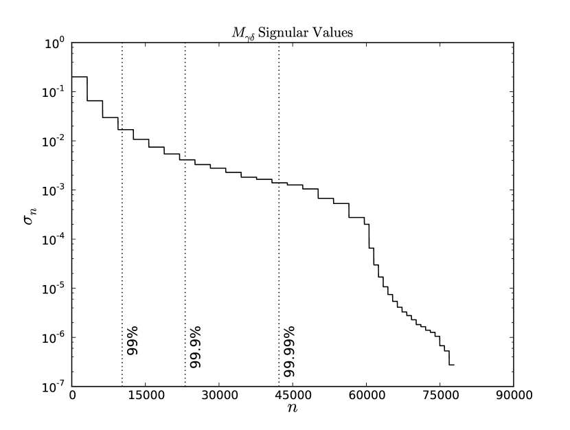
Figure 1.— Ordered singular values of the matrix $\widetilde{M_{\gamma\delta}}$. The dotted lines show the values of $n$ such that 99%, 99.9%, and 99.99% of the variance is preserved. The sharp drop-off near $n=60,000$ is due to the $10^{-3}$ deweighting of border pixels.

3. Results

Using the above formalism, we can now explore the tomographic weak lensing problem using the techniques of Section 2. For the following discussion, we will use a field of approximately one square degree: a $64\times 64$ grid of $1^{\prime}\times 1^{\prime}$ pixels, with 25 source redshift bins ($0\leq z\leq 2.0$, $\Delta z=0.08$) and 20 lens redshift bins ($0\leq z\leq 2.0$, $\Delta z=0.1$). This binning approximates the expected photometric redshift errors of future surveys. We suppress edge effects by increasing the noise of all pixels within $4^{\prime}$ of the field border by a factor of $10^{3}$, effectively deweighting the signal in these pixels (cf. STH09). The noise for each redshift bin is set to $n_{i}=\sigma_{\gamma}/\sqrt{N_{i}}$, where $\sigma_{\gamma}$ is the intrinsic ellipticity dispersion, and $N_{i}$ is the number of galaxies in the bin. We assume $\sigma_{\gamma}=0.3$, and 70 galaxies per square arcminute, with a redshift distribution given by

$$n(z)\propto z^{2}\exp{\left[-(z/z_{0})^{3/2}\right]},$$ (9)

with $z_{0}=0.57$. We assume a flat cosmology with $h=0.7$, $\Omega_{M}=0.27$ and $\Omega_{\Lambda}=0.73$ at the present day.

3.1. Singular Values

The singular values of the transformation matrix for this configuration are depicted in Figure 1. The step pattern visible in this plot is due to the fact that the noise across each source plane is identical, aside from the $4^{\prime}$ deweighted border. It is apparent from this figure that the large majority of the singular values are very small: 99.9% of the variance in the transformation is contained in less than $1/3$ of the singular values. The large number of very small singular values will, therefore, dominate in the Aitken estimator (Equation 4), leading to the very noisy unfiltered results seen in HK02.

3.2. Evaluation of the SVD Estimator

To evaluate the performance of the SVD filter, we first create a field-of-view containing a single halo at redshift $z=0.6$. One well-supported parametrization of halo shapes is the NFW profile (Navarro et al., 1997). We use the analytic form of the shear and projected density due to an NFW profile, given by equations 13-18 in Takada & Jain (2003).

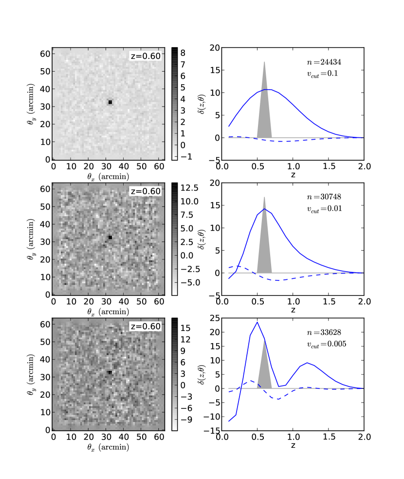
Figure 2.— The effect of SVD truncation on a single $z=0.6$ NFW halo in the center of the field, for three different levels of filtering. left column: reconstructed density parameter $\delta(\theta)$ in the $z=0.6$ lens-plane. The true matter distribution is represented by a tight “dot” in the center of the plot. right column: line-of-sight profile at the central pixel. The grey shaded area shows the input density parameter. The solid line shows the E-mode signal, while the dashed line shows the B-mode signal. $n$ gives the number of singular values used in the reconstruction (out of a total $n_{\rm max}=81920$), and $v_{\rm cut}$ gives the amount of variance cut by the truncation (Equation 8); the level of filtration decreases from the top panels to the bottom panels. The bottom panels show a case of under-filtering: for small enough $v_{\rm cut}$, the noise overwhelms the signal and creates spurious peaks along the line-of-sight.

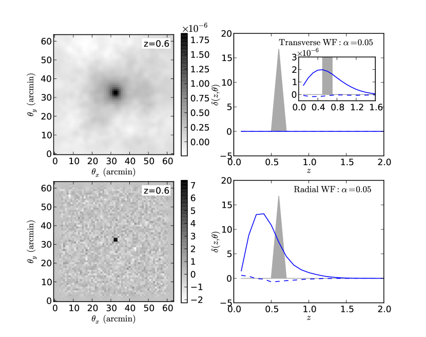
Figure 3.— The effect of Wiener filtering on the same input as Figure 2. Here we have used both transverse (top panels) and radial (bottom panels) Wiener filtering, both down-tuned by $\alpha=0.05$ (the value recommended by STH09). The transverse Wiener filter suppresses the response by several orders of magnitude; a closer view of the line-of-sight peak is shown in the inset plot. The radial Wiener filter gives similar angular results to the SVD filter, but takes much longer to compute.

We reconstruct the density map using the SVD filter (Figure 2) with the above survey parameters. We show the results for three different values of $v_{\rm cut}$: 0.1, 0.01, and 0.005. In all three cases, the halo is easily detected at its correct location (left panels), although as $v_{\rm cut}$ decreases, there is more noise in the surrounding field. The right panels show the computed density profile along the line of sight for the central pixel. The peak of this curve is reasonably close to the correct redshift, but there is a significant spread in redshift, as well as a bias. As the level of SVD filtering (measured by $v_{\rm cut}$) decreases, the magnitude of these effects decreases, but the increased noise leads to spurious peaks.

Similar plots for the transverse Wiener filter recommended by STH09 are shown in the upper panels of Figure 3, using their recommended value of $\alpha=0.05$. The response shows a significant spread in angular space, and the signal is seen to be suppressed by six orders-of-magnitude along with a similar suppression of the noise. These effects worsen, in general, as the filtering level $\alpha$ increases. Mathematically it is apparent why the transverse filter performs so poorly: the small singular values primarily come from the line-of-sight part of the mapping, and the this filter has no effect along the line-of-sight.

The effect of the radial Wiener filter is shown in the bottom panels of Figure 3. It shares the positive aspects of the SVD filter, having very little signal suppression or angular spread. However, this filter uses some priors on the statistical form of the signal that are not as physically well-motivated as those for the transverse Wiener filter. In contrast, the SVD filter does not make any prior assumptions about the signal. In this way, the SVD reconstruction can be thought of as even more non-parametric than the Wiener filter reconstructions.

3.3. Comparison of Estimators

The SVD framework laid out in Section 2.2 can be used to quantitatively compare the behavior of different estimators. A general linear estimator has the form

$$\boldsymbol{\hat{\delta}_{R}}=R\boldsymbol{\gamma}$$ (10)

for some matrix $R$. This general estimator can be expressed in terms of the components of the unbiased estimator (Equation 4):

$$R=V_{R}\Sigma^{-1}U^{\dagger}\mathcal{N}_{\gamma\gamma}^{-1/2}.$$ (11)

Here the matrices $\Sigma$, $U$ and $\mathcal{N}_{\gamma\gamma}$ are defined as in Equation 4, and we have defined the matrix

$$V_{R}\equiv R\mathcal{N}_{\gamma\gamma}^{1/2}U\Sigma$$ (12)

The rows of the matrix $\Sigma^{-1}U^{\dagger}\mathcal{N}_{\gamma\gamma}^{-1/2}$ provide a convenient basis in which to work: they are the weighted principal components of the shear, ordered with decreasing signal to noise. The norm of the $i^{\rm th}$ column of $V_{R}$ measures the contribution of the $i^{\rm th}$ mode to the reconstruction of $\delta$. For the unfiltered estimator, $V_{R}=V$ and all the norms are unity. This leads to a very intuitive comparison between different filtering schemes. Figure 4 compares the column-norms of $V_{R}$ for the SVD filter with those of the radial and transverse Wiener filters.

The steps visible in the plot originate the same way as the steps in Figure 1: the flatness of each step comes from the assumption of uniform noise in each source plane. This plot shows the tradeoff between noise and bias. The flat line at norm=$10^{0}$ represents a noisy but unbiased estimator. Any departure from this will impose a bias, but can increase signal-to-noise. There are two important observations from this figure. First, because each step on the plot is relatively flat for the SVD filter and radial Wiener filter, we don’t expect much bias within each lens plane. The transverse filter, on the other hand, has fluctuations at the $10\%$ level within each step (visible in the inset of Figure 4), which will lead to a noticeable bias within each lens plane, resulting in the degraded angular resolution of the reconstruction seen in Figure 3. Second, the transverse Wiener filter deweights even the highest signal-to-noise modes by many orders of magnitude, resulting in the signal suppression seen in Figure 3. The SVD filter and radial Wiener filter, on the other hand, have weights near unity for the highest signal-to-noise modes. These two observations show why the SVD filter and radial Wiener filter are the more successful noise reduction techniques for the present problem.

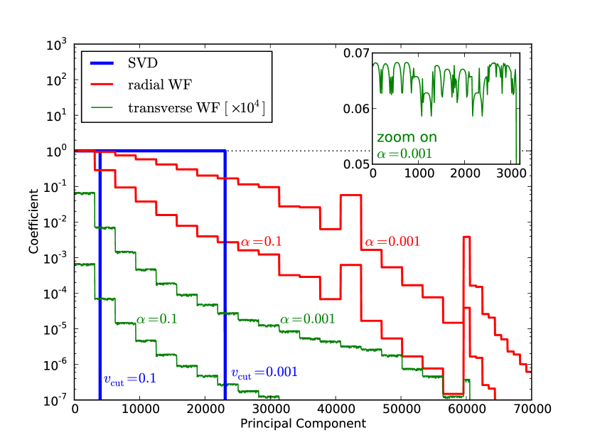
Figure 4.— Contribution of each shear mode to the reconstruction for three different filters. The dotted line at $10^{0}$ represents the unfiltered result. Each filtering method leads to a different weighting of the shear modes. The SVD filter, by design, completely removes higher-order modes beyond a given cutoff, while the Wiener filter deweights modes in a more gradual fashion. Note that the transverse Weiner filter deweights all modes by up to seven orders of magnitude; it has been scaled by a factor of $10^{4}$ for this plot. The inset plot shows a closeup of the fluctuations within each “step” of the transverse filter. These fluctuations lead to angular spread in the response (see discussion in Section 3.3)

3.4. Noise Properties of Line-of-Sight Modes

As seen in equation 5, the columns of $V$ provide a natural orthogonal basis in which to express the signal $\boldsymbol{\delta}$. It should be emphasized that this eigenbasis is valid for any linear filtering scheme: the untruncated SVD is simply an equivalent re-expression of the original transformation. Examining the characteristics of these eigenmodes can yield insight regardless of the filtering method used.

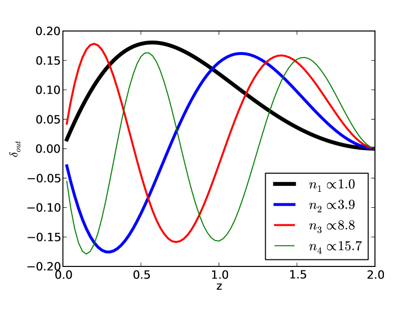
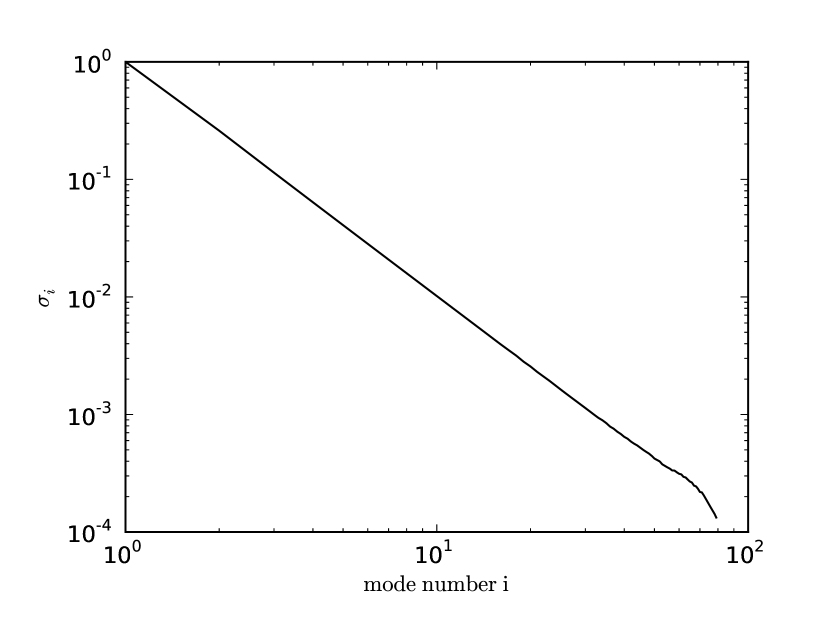
Figure 5.— left panel: The radial components of the first four columns of the matrix $V$ (see section 2.1). This is calculated for 100 equally spaced redshift bins $(0\leq z\leq 2.5)$ in $\boldsymbol{\gamma}$, and 80 bins $(0\leq z\leq 2.0)$ in $\boldsymbol{\delta}$ These orthogonal eigenmodes are analogous to radial Fourier modes. Each is labeled by its relative noise level, $n_{i}=(\sigma_{i}/\sigma_{1})^{-1}$. right panel: The singular values $\sigma_{i}$ associated with the 80 radial eigenmodes.

The radial components of the first four eigenmodes are plotted in figure 5. Each is labeled by its normalized noise level, $n_{i}\equiv(\sigma_{i}/\sigma_{1})^{-1}$. The total number of modes will be equal to the number of output redshift bins; here, for clarity, we’ve used 80 equally-spaced bins out to redshift 2.0. As the resolution is lessened, the overall shape and relative noise level of the lower-order modes is maintained. These radial modes are analogous to angular Fourier modes, and are related to the signal-to-noise KL modes discussed in HK02. It is clear from this plot that any linear, non-parametric estimator will be fundamentally limited in its redshift resolution: the noise level of the $i^{th}$ mode approximately scales as

$$n_{i}\ \widetilde{\propto}\ i^{2}$$ (13)

The signal-to-noise level for any particular halo will depend on its mass and redshift. The magnitude of the signal scales linearly with mass (see discussion in STH09), but the redshift dependence is more complicated: it is affected by the lensing efficiency function, which depends on the redshift of the lensed galaxies. Using the above survey parameters, with an NFW halo of mass $M_{200}=10^{15}\rm{M_{\odot}}$ and redshift $z=0.6$, the signal-to-noise ratio of the central pixel for the fundamental radial mode is $\sim 5.9$, consistent with the results for Wiener filtered reconstructions of singular isothermal halos explored in STH09. This means that for even the largest halos, with a very deep survey, only the first few modes will contribute significantly to the reconstructed halo. Adding higher-order modes can in theory provide redshift information, but at the cost of increasingly high noise contamination. This is a general result which will apply to all nonparametric linear reconstruction algorithms.

This lack of information in the redshift direction leads directly to an inability to accurately determine halo masses: the lensing equations relate observed shear $\gamma$ to density parameter $\delta$, which is related to mass in a redshift-dependent way. This is a fundamental limitation on the ability of linear nonparametric methods to determine halo masses from shear data. Indeed, even moving to fully parametric models, line-of-sight effects can lead to halo mass errors of 20% or more (Hoekstra, 2003; de Putter & White, 2005).

3.5. Reconstruction of a Realistic Field

To compare the performance of the three filtering methods for a realistic field, we create a 4 square degree field with approximately 20 halos between masses of $2\times 10^{14}$ and $8\times 10^{14}{\rm M_{\odot}}$ with a mass distribution approximating the cluster mass function of Rines et al. (2007), and a redshift distribution given by Equation 9, adding a hard cutoff at $z=1.0$. These parameters are chosen to approximate the true distribution of observable halos in a field this size. The results of the reconstruction are shown in Figure 6

The red circles are the locations of the input halos, not the result of some halo-detection algorithm. However, it is clear that, for at least most of the mass range, we are able to produce a map for which any reasonable detection algorithm should detect the halos in the correct locations. A few of the lower mass halos would certainly be missed though, since they are not significantly different from the noise peaks in the image.

In practice, one may vary the parameter $v_{\rm cut}$ as in Figure 2 to trade-off robustness of detecting peaks with resolution in angle and in redshift. As shown in Section 3.3, we expect filtering to introduce very little bias in angular resolution, so large values of $v_{\rm cut}$ lead to the most robust angular results. On the other hand, as shown in Section 3.4, filtering introduces an extreme bias along the line-of-sight. The effects of this bias can be seen qualitatively in the right column of Figure 2. Optimal redshift resolution requires choosing a filtering level which balances the effects of noise and bias, and may require some form of bias correction. In future work, we will explore in detail the ways in which the SVD method allows for a near optimal reconstruction of projected mass maps and halo redshifts from data on galaxy shapes and photometric redshifts.

3.6. Scalability

As we look forward to future surveys, it becomes important to consider methods that will scale upward with increasing survey volumes. Present weak lensing surveys cover fields on the order of a few square degrees (e.g. COSMOS, Massey et al., 2007). Future surveys will increase the field size exponentially: up to $\sim\!\!20,000$ square degrees for LSST (LSST Science Collaborations et al., 2009). Though the flat-sky approximation used in this work is not appropriate for such large survey areas, the weak lensing formalism can be modified to account for spherical geometry (see, e.g. Heavens, 2003).

The main computational cost for both SVD and Wiener filtering is the Fast Fourier Transform (FFT) required to implement the mapping from $\gamma$ to $\kappa$. For an $N\times N$ pixel field, the FFT algorithm performs in $\mathcal{O}[N\log N]$ in each dimension, meaning that the 2D FFT takes $\mathcal{O}[(N\log N)^{2}]\approx\mathcal{O}[N^{2}]$. The Wiener filter method, however, requires the inversion of a very large matrix using, for example, a conjugate-gradient method. The exact number of iterations depends highly on the condition number of the matrix to be inverted; STH09 finds that up to 150 iterations are required for this problem. We find that each iteration takes over 3 times longer than the entire SVD reconstruction. The net result is that both algorithms scale nearly linearly with the area of the field (for constant pixel scale), though the SVD estimator is computed up to 500 times faster than the Wiener filter.

Extrapolating this scaling, the appropriately scaled SVD filter will allow reconstruction of the entire $\sim\!\!20,000$ square-degree LSST field in a few hours on a single workstation, given enough memory. On the same computer, the Wiener-filter method would take over a month, depending on the amount and type of filtering and assuming that the required number of iterations stays constant with increasing field size. For the SVD-filtered reconstruction of this large field, the real challenge will not be computational time, but memory constraints: the complex shear vector itself for such a field will require $\sim\!\!30$ GB of memory, with the entire algorithm consuming approximately three times this. The memory requirements for the Wiener filter will be comparable. This is within reach of current high-end workstations as well as shared-memory parallel clusters.

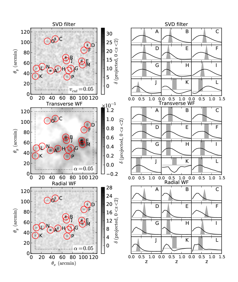
Figure 6.— Reconstruction of an artificial shear field with the SVD filter (top panels), Transverse Wiener filter (middle panels), and Radial Wiener filter (bottom panels). The left column shows the projected density reconstruction across the field using each method, all smoothed with a 1-pixel wide Gaussian filter. Red circles indicate the true locations of the input halos. The right column shows the line-of-sight distributions of the twelve most massive NFW halos, labeled A-L. The masses and redshifts of the halos are listed in Table 1. The signal suppression of the transverse Wiener filter seen in Figure 3 is apparent in the color-bar scaling of the middle panels. The anomalous results seen in halo K are due to its proximity to the deweighted border. As suggested by the discussion in Section 3.4, none of the three methods succeed in recovering precise redshifts of the halos.

Table 1Masses and redshifts of halos in Figure 6.

	$\theta_{x}$	$\theta_{y}$	$z$	$M/M_{\odot}$
A	37.5	44.9	0.60	$7.2\times 10^{14}$
B	67.1	70.5	0.47	$6\times 10^{14}$
C	46.9	106.5	0.63	$5.5\times 10^{14}$
D	108.9	94.3	0.63	$5.4\times 10^{14}$
E	97.9	63.6	0.39	$4.9\times 10^{14}$
F	102.4	84.8	0.70	$3.8\times 10^{14}$
G	77.0	49.6	0.58	$3.2\times 10^{14}$
H	52.0	48.5	0.36	$3.2\times 10^{14}$
I	72.6	45.6	0.78	$2.9\times 10^{14}$
J	68.6	64.5	0.68	$2.5\times 10^{14}$
K	8.6	34.5	0.32	$2.3\times 10^{14}$
L	10.5	49.5	0.51	$2.3\times 10^{14}$
M	99.4	56.5	0.22	$2.3\times 10^{14}$
N	21.7	53.1	0.76	$2.3\times 10^{14}$
O	31.6	102.1	0.69	$2.2\times 10^{14}$
P	69.7	33.2	0.39	$2.2\times 10^{14}$

4. Conclusion

We have presented a new method for producing tomographic maps of dark matter through weak lensing, using truncation of singular values. We have tested and compared our method to the Wiener filter based method of STH09, which is the first three-dimensional mass mapping approach that is applicable to large area surveys. Our reconstruction shares many of the aspects of the Wiener filter reconstruction, in the sense that it massively reduces the noise inherent in the problem. Our SVD method may be considered even more non-parametric than the Wiener filter method, since it does not rely on any a priori assumptions of the statistical properties of the signal: all of the noise reduction is derived from the observed noise properties of the data.

The SVD framework allows a unique quantitative comparison between the different filtering methods and filtering strengths. Using the coefficients of the weighted principal components contained in the SVD, we have compared the three filtering methods, and have found that the radial Wiener filter of HK02 and SVD filter of this work are less-biased noise reduction techniques than the transverse Wiener filter of STH09. These authors have recently implemented the radial Weiner filter and obtain results consistent with our findings (P. Simon and A. Taylor, private communication).

The angular resolution of the SVD-reconstructed mass maps seems to be significantly better than that of the transverse Wiener filter method, the method chosen in the STH09 analysis. This allows for more robust separation of pairs of halos into two separate halos rather than blurring them into a single mass peak. We discuss how our reconstruction method provides a scheme for optimizing the 3D reconstruction of projected mass maps by balancing the goals of robustness of detecting specific structures and improved redshift resolution.

The SVD method can compute the three-dimensional mass maps rapidly provided sufficient computational memory is available. This allows for the possibility of solving the full-sky tomographic lensing inversion on the scale of hours, rather than months, which makes it readily applicable to upcoming surveys.

On the other hand, the redshift resolution with the SVD method is not significantly better than that of either Wiener filter method. This was a problem identified by STH09, and unfortunately the SVD method does not significantly improve the situation. Our analysis of the noise characteristics of radial modes indicates that linear, non-parametric reconstruction methods are fundamentally limited in this regard.

Acknowledgments: We are grateful to Patrick Simon and Andy Taylor for numerous discussions and insights on the Wiener filter method, which helped improve our study. We thank the anonymous referee for several helpful suggestions. Support for this research was provided by NASA Grant NNX07-AH07G. We acknowledge partial support from NSF AST-0709394.

Appendix A Efficient Implementation of the SVD Estimator

As noted in Section 2.2, taking the SVD of the transformation matrix $\widetilde{M}_{\gamma\delta}\equiv\mathcal{N}_{\gamma\gamma}^{-1/2}M_{\gamma\delta}$ is not trivial for large fields. This appendix will first give a rough outline of the form of $M_{\gamma\delta}$, then describe our tensor decomposition method which enables quick calculation of the singular value decomposition. For a more thorough review of the lensing results, see e.g. Bartelmann & Schneider (2001).

Our goal is to speed the computation of the SVD by writing  $\widetilde{M}_{\gamma\delta}$ as a tensor product $A\otimes B$. Here “$\otimes$” is the Kronecker product, defined such that, if $A$ is a matrix of size $n\times m$, $B$ is a matrix of arbitrary size,

$$A\otimes B\equiv\left(\begin{array}[]{cccc}A_{11}B&A_{12}B&\cdots&A_{1m}B\\ A_{21}B&A_{22}B&\cdots&A_{2m}B\\ \vdots&\vdots&\ddots&\vdots\\ A_{n1}B&A_{n2}B&\cdots&A_{nm}B\end{array}\right)$$ (A1)

In this case, the singular value decomposition $A\otimes B=U_{AB}\Sigma_{AB}V^{\dagger}_{AB}$ satisfies

$$U_{AB} = U_{A}\otimes U_{B}$$

$$\Sigma_{AB} = \Sigma_{A}\otimes\Sigma_{B}$$

$$V_{AB} = V_{A}\otimes V_{B}$$ (A2)

where $U_{A}\Sigma_{A}V^{\dagger}_{A}$ is the SVD of $A$, and $U_{B}\Sigma_{B}V^{\dagger}_{B}$ is the SVD of $B$. Decomposing $\widetilde{M}_{\gamma\delta}$ in this way can greatly speed the SVD computation.

A.1. Angular and Line-of-Sight Transformations

The transformation from shear to density, encoded in $M_{\gamma\delta}$, consists of two steps: an angular integral relating shear $\gamma$ to convergence $\kappa$, and a line-of-sight integral relating the convergence $\kappa$ to the density contrast $\delta$.

The relationship between $\gamma$ and $\kappa$ is a convolution over all angular scales,

$$\gamma(\boldsymbol{\theta},z_{s})\equiv\gamma_{1}+i\gamma_{2}=\int\mathrm{d}^{2}\theta^{\prime}\ \mathcal{D}(\boldsymbol{\theta}^{\prime}-\boldsymbol{\theta})\kappa(\boldsymbol{\theta}^{\prime},z_{s}),$$ (A3)

where $\mathcal{D}(\boldsymbol{\theta})$ is the Kaiser-Squires kernel (Kaiser & Squires, 1993). This has a particularly simple form in Fourier space:

$$\hat{\gamma}(\boldsymbol{\ell},z_{s})=\frac{\ell_{1}+i\ell_{2}}{\ell_{1}-i\ell_{2}}\hat{\kappa}(\boldsymbol{\ell},z_{s}).$$ (A4)

where $\hat{\gamma}$ and $\hat{\kappa}$ are the Fourier transforms of $\gamma$ and $\kappa$ and $\boldsymbol{\ell}\equiv(\ell_{1},\ell_{2})$ is the angular wavenumber.

The relationship between $\kappa$ and $\delta$ is an integral along each line of sight:

$$\kappa(\boldsymbol{\theta},z_{s})=\int_{0}^{z_{s}}\mathrm{d}z\ W(z,z_{s})\delta(\boldsymbol{\theta},z)$$ (A5)

where $W(z,z_{s})$ is the lensing efficiency function at redshift $z$ for a source located at redshift $z_{s}$ (refer to STH09 for the form of this function).

Upon discretization of the quantities $\gamma$, $\kappa$, and $\delta$ (described in Section 2.1), the integrals in Equations A3-A5 become matrix operations. The relationship between the data vectors $\boldsymbol{\gamma}$ and $\boldsymbol{\kappa}$ can be written

$$\boldsymbol{\gamma}=[P_{\gamma\kappa}\otimes\mathbf{1}_{s}]\boldsymbol{\kappa}+\boldsymbol{n}_{\gamma}$$ (A6)

where $\mathbf{1}_{s}$ is the $N_{s}\times N_{s}$ identity matrix and $P_{\gamma\kappa}$ is the matrix representing the linear transformation in Equations A3-A4. The quantity $[P_{\gamma\kappa}\otimes\mathbf{1}_{s}]$ simply denotes that $P_{\gamma\kappa}$ operates on each of the $N_{s}$ source-planes represented within the vector $\boldsymbol{\kappa}$. Similarly, the relationship between the vectors $\boldsymbol{\kappa}$ and $\boldsymbol{\delta}$ can be written

$$\boldsymbol{\kappa}=[\mathbf{1}_{xy}\otimes Q_{\kappa\delta}]\boldsymbol{\delta}$$ (A7)

where $\mathbf{1}_{xy}$ is the $N_{xy}\times N_{xy}$ identity matrix, and the tensor product signifies that the operator $Q_{\kappa\delta}$ operates on each of the $N_{xy}$ lines-of-sight in $\boldsymbol{\delta}$. $Q_{\kappa\delta}$ is the $N_{s}\times N_{l}$ matrix which represents the discretized version of equation A5. Combining these representations allows us to decompose the matrix $M_{\gamma\delta}$ in Equation 1 into a tensor product:

$$M_{\gamma\delta}=P_{\gamma\kappa}\otimes Q_{\kappa\delta}.$$ (A8)

A.2. Tensor Decomposition of the Transformation

We now make an approximation that the noise covariance $\mathcal{N}_{\gamma\gamma}$ can be written as a tensor product between its angular part $\mathcal{N}_{P}$ and its line of sight part $\mathcal{N}_{Q}$:

$$\mathcal{N}_{\gamma\gamma}=\mathcal{N}_{P}\otimes\mathcal{N}_{Q}.$$ (A9)

Because shear measurement error comes primarily from shot noise, this approximation is equivalent to the statement that source galaxies are drawn from a single redshift distribution, with a different normalization along each line-of-sight. For realistic data, this approximation will break down as the size of the pixels becomes very small. We will assume here for simplicity that the noise covariance is diagonal, but the following results can be generalized for non-diagonal noise. Using this noise covariance approximation, we can compute the SVDs of the components of $\widetilde{M}_{\gamma\delta}$:

$$U_{P}\Sigma_{P}V_{P}^{\dagger}=\mathcal{N}_{P}^{-1/2}P_{\gamma\kappa}$$

$$U_{Q}\Sigma_{Q}V_{Q}^{\dagger}=\mathcal{N}_{Q}^{-1/2}Q_{\kappa\delta}$$ (A10)

In practice the SVD of the matrix $P_{\gamma\kappa}$ need not be computed explicitly. $P_{\gamma\kappa}$ encodes the discrete linear operation expressed by Equations A3-A4: as pointed out by STH09, in the large-field limit $P_{\gamma\kappa}$ can be equivalently computed in either real or Fourier space. Thus to operate with $P_{\gamma\kappa}$ on a shear vector, we first take the 2D Fast Fourier Transform (FFT) of each source-plane, multiply by the kernel $(\ell_{1}+i\ell_{2})/(\ell_{1}-i\ell_{2})$, then take the inverse FFT of the result. This is orders-of-magnitude faster than a discrete implementation of the real-space convolution. Furthermore, the conjugate transpose of this operation can be computed by transforming $\ell\to-\ell^{*}$, so that

$$P_{\gamma\kappa}^{\dagger}P_{\gamma\kappa}=I$$ (A11)

and we see that $P_{\gamma\kappa}$ is unitary in the wide-field limit. This fact, along with the tensor product properties of the SVD, allows us to write $\widetilde{M}_{\gamma\delta}=U\Sigma V^{\dagger}$ where

$$U \approx \mathbf{1}_{xy}\otimes U_{Q}$$

$$\Sigma \approx \mathcal{N}_{P}^{-1/2}\otimes\Sigma_{Q}$$

$$V^{\dagger} \approx P_{\gamma\kappa}\otimes V_{Q}^{\dagger}$$ (A12)

The only explicit SVD we need to calculate is that of $\mathcal{N}_{Q}^{-1/2}Q_{\kappa\delta}$, which is trivial in cases of interest. The two approximations we have made are the applicability of the Fourier-space form of the $\gamma\to\kappa$ mapping (Eqn. A4), and the tensor decomposition of the noise covariance (Eqn. A9).

References

- Aitken (1934) Aitken, A. 1934, Proc. R. Soc. Edinb, 55, 42
- Bacon & Taylor (2003) Bacon, D. J., & Taylor, A. N. 2003, MNRAS, 344, 1307
- Bartelmann & Schneider (2001) Bartelmann, M., & Schneider, P. 2001, Phys. Rep., 340, 291
- Clowe et al. (2006) Clowe, D., Bradač, M., Gonzalez, A. H., Markevitch, M., Randall, S. W., Jones, C., & Zaritsky, D. 2006, ApJ, 648, L109
- de Putter & White (2005) de Putter, R., & White, M. 2005, New A, 10, 676
- Heavens (2003) Heavens, A. 2003, MNRAS, 343, 1327
- Hoekstra (2003) Hoekstra, H. 2003, MNRAS, 339, 1155
- Hu & Keeton (2002) Hu, W., & Keeton, C. R. 2002, Phys. Rev. D, 66, 063506
- Kaiser & Squires (1993) Kaiser, N., & Squires, G. 1993, ApJ, 404, 441
- LSST Science Collaborations et al. (2009) LSST Science Collaborations et al. 2009, ArXiv e-prints
- Massey et al. (2007) Massey, R., et al. 2007, ApJS, 172, 239
- Navarro et al. (1997) Navarro, J. F., Frenk, C. S., & White, S. D. M. 1997, ApJ, 490, 493
- Rines et al. (2007) Rines, K., Diaferio, A., & Natarajan, P. 2007, ApJ, 657, 183
- Simon et al. (2009) Simon, P., Taylor, A. N., & Hartlap, J. 2009, MNRAS, 399, 48
- Takada & Jain (2003) Takada, M., & Jain, B. 2003, MNRAS, 344, 857
- Taylor (2001) Taylor, A. N. 2001, ArXiv Astrophysics e-prints