Quantized Black Hole and Heun function

Abstract

Abstract

Following the simple proposal by He and Ma for quantization of a black hole(BH) by Bohr’s idea about the atoms,we discussed the solvability of the wave equation for such a BH. We superficial solved the associated Schrodinger equation. The eigenfunction problem reduces to HeunB $H$ differential equation which is a natural generalization of the hypergeometric differential equation. In other words, the spectrum can be determined by solving the Heun s differential equation.

I Introduction

In 2010,Verlinde inspired directly from the Holography conceptHooft ; Susskind ,proposed an idea Verlinde about the quantum origin of the gravity and the second law of inertia. In this scenario, the key objects are the concept of the change in entropy stored on the holographic screen, when the test particle moves toward the screen and the entropic force comes from the polymer physics. In the simplest form, the entropic force try to recover the Newton’s gravitational theory and it has been shown that why we can believe to gravity as an thermodynamical quantity. There are many papers in literatures about this idea and it’s possible extensions entropic . The simple mathematics behind entropic scenarion excited many disputations about the validity of it’s arguments. Essentially the relation between thermodynamics and the black hole physics is an old ideabekenstein ; hawking and indeed there is a deep relation between general relativity (GR) and thermodynamical structure of the field eqsjacobson ; paddy . It has been proved that the Einstein field equations avaluated on the horizon can be interpreted as the first law of the thermodynamics for BH. Discovering of the Hawking radiation and the famous area-entropy formula for BHs and it’s extensions to the power law and logarithmic corrected entropy function opened new windows to the new abilities to demeaning the BH horizon as a thermodynamical system sustained this conjecture. If we accept the Velinde idea ,a test particle which obeys from the uncertainly principle near to a holographic screen (which is an equipotential surface) changes the entropy of the screen slightly and as which is argued original by Verlinde this amount of the entropy which is proportional to the displacement, causes a force which is responsible for the attractive force between the test particle and the screen. Some problems as the locality of the energy and the temperature remain unsolved. For example it is difficult to interpret in any arbitrary case the Unruh temperature of the accelerated observer exactly in the same manner as the horizon temperature $T_{BH}$. Some authors showed that the simple form of the gravitational force in the verlinde idea is not unique, and by taking some additional terms which each term causes some corrections to the BH entropy formula, for example the log corrections or volume corrections Modesto . Such kinds of the entropy corrections come from the LQG LQG ,and the similarity of the new force terms to the MOND approachMOND ,all of them show us that (may be) we work in an equivalent formulation. The quantum corrections to the Newton’s gravitation law and the unfamiliar and strange uncertainty principle arisen from it,all are lugubrious. Anyway ,from many papers on this topics one which acclaimed about the quantization of the BH, attracted us. In HeMa the authors under simple conditions and from the Bohr’s quantization, construct some expression for the energy, the surface area, the Compton’s wavelength, the surface gravity, quantized temperature. We do not repeat their results and referring the reader to the HeMa . In this work we want to calculate the wave function for this quantized energy spectrum of the BH area. We assume that this energy spectrum (which possesses also low energy continuum behavior),corresponds to a particle with mass of order Planck mass and it’s radial potential varies by a power of $\frac{2}{3}$. The wave function will be calculated in terms of the more complicated functions as the usual quantum mechanical radial wave functions.

The plan of this paper is as follow. In section II we obtain the potential function using WKB method. In section III we solve the wave equation using the series method. In section IV we apply the Poincare asymptotic method to recover the exact wave function. In section V we calculate the expectation values of the kinetic and potential energies using Hellmann Feynman theorem. We summarize and conclude in last section.

II The general potential for a test particle with energy spectrum $E_{n}=M_{p}c^{2}\sqrt{n}$

As it was stated by He-Ma,the general energy spectrum for a quantized BH is relationHeMa :

$$\begin{aligned} E_{n}=M_{p}c^{2}\sqrt{n}.\end{aligned}$$ (1)

We know that the Bohr scenario for quantization of a Hydrogen atom is valid only in large quantum numbers,namely it is the asymptotic limit of the general WKB approximation. As a simple consequence of imposing the Bohr-Sommerfeld quantization to a general potential function both one dimensional or completely spherically symmetric ones,we know that this energy spectrum can be produced from the following potential function

$$\begin{aligned} V=V_{0}|\overrightarrow{r}|^{p}\Rightarrow E_{n}\approx n^{\frac{2p}{p+2}}\end{aligned}$$ (2)

reminiscence the validity of (1) in the large quantum numbers $n$ and comparing to the (2),we deduce that the general potential term must be

$$\begin{aligned} V=V_{0}|\overrightarrow{r}|^{\frac{2}{3}}.\end{aligned}$$ (3)

The potential function (3) is not bound. In Figure 1 we plot the potential function. It shows that in the semi classical limit if the BH want to remains stable, firstly the matter waves must be standing waves and no bound states is needed for such a quantized BH.

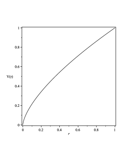
Figure 1: The potential function $V(r)$ for a particle in the quantized BH.

III Schrödinger wave equation

In this section we will solve the wave equation for a quantized BH. We assume that the BH behaves like a paricle with mass $M$ ,and write the static wave functions $\phi(r,\theta,\phi)=\frac{u(r)}{r}Y_{lm}(\theta,\phi)$,in usual spherically symmetric coordinates and a normal separation of the variables,we obtain the radial equation

$$\begin{aligned} -\frac{\hbar^{2}}{2M}u^{\prime\prime}+(\frac{\hbar^{2}l(l+1)}{2Mr^{2}}+V_{0}r^{\frac{2}{3}}-M_{p}c^{2}\sqrt{n})u=0.\end{aligned}$$ (4)

It is adequate to introducing a new set of variable $x=\alpha r$ where $\alpha=(\frac{2MV_{0}}{\hbar^{2}})^{\frac{3}{8}}$ and a new parameter $b=M_{p}c^{2}(\frac{2M}{\hbar^{2}V_{0}^{3}})^{\frac{1}{4}}$. In these variables we obtain

$$\begin{aligned} \frac{d^{2}u}{dx^{2}}+(-\frac{l(l+1)}{x^{2}}-x^{\frac{2}{3}}+b\sqrt{n})u=0.\end{aligned}$$ (5)

The general solution for this diffrential equation,is in the form of HeunB functions denoted by $H$ Heun multiplied by some functions

$$\begin{aligned} u(x)=e^{-f_{n}}\Big{[}c_{1}x^{-l}H(-\frac{3}{2}-3l,b\sqrt{\frac{3n}{2}},\frac{3}{8}nb^{2},0,-\frac{3}{2}x^{2/3})+c_{2}x^{l+1}H(\frac{3}{2}+3l,b\sqrt{\frac{3n}{2}},\frac{3}{8}nb^{2},0,-\frac{3}{2}x^{2/3})\Big{]}\end{aligned}$$ (6)

where

$$\begin{aligned} f_{n}=-\frac{3}{4}x^{\frac{3}{2}}(x^{\frac{3}{2}}-b\sqrt{n}).\end{aligned}$$ (7)

In Figure 2, we plot the function $f_{n}$ as a function of $x$ with $b=1$ for diffrent values of n.

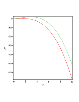
Figure 2: The $f_{n}$ function for $n=10(Red),100(Green)$.

We can set $c_{2}=0$ for square integrability of the wave function. Thus the total wave function is:

$$\begin{aligned} \phi(x,\theta,\phi)=Ne^{-f_{n}}x^{-l-1}H(\pm(\frac{3}{2}+3l),b\sqrt{\frac{3n}{2}},\frac{3}{8}nb^{2},0,-\frac{3}{2}x^{2/3})Y_{lm}(\theta,\phi)\end{aligned}$$ (8)

In Figure 3, we plot the radial wave function $u(x)$ for some values of the parameters.

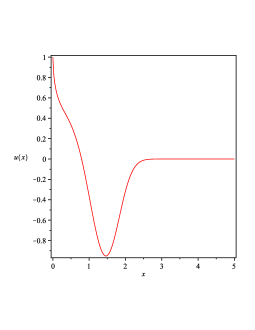
Figure 3: The normalizable radial function $u(x)$ for s-wave $l=0,n=10$ , $b=\sqrt{\frac{2}{3}}$.

IV Poincare’s Asymptotic method

We write out the local expansion of the coefficients of Eq. (5) near a regular singularity $x=\infty$:

$$\begin{aligned} u^{\infty}(x)=Ax^{1/2}Z_{\frac{3}{8}}\Big{(}\frac{3}{4}x^{\frac{4}{3}}\Big{)},\end{aligned}$$ (9)

Where the $Z_{\nu}(ax)$ is apiece of the Bessel functions of the second kind. Also we introduce a pair of Frobenius solutions in a neighborhood of an apparent singularity $x=0$ that is fixed by the following behavior:

$$\begin{aligned} u_{0}(x)=c_{1}x^{-l}+c_{2}x^{l+1}.\end{aligned}$$ (10)

Note that apparent singular points $x=0,\infty$ play an important role in general monodromy properties of linear Fuchsian systems.
Now we suppose that the general solution for (5) is

$$\begin{aligned} u(x)=Ax^{\frac{3}{2}+l}Z_{\frac{3}{8}}\Big{(}\frac{3}{4}x^{\frac{4}{3}}\Big{)}y(x).\end{aligned}$$ (11)

Remember to mind that in the asymptotic regime $x=\infty$ we have

$$\begin{aligned} Z_{\frac{3}{8}}\Big{(}ax^{\frac{4}{3}}\Big{)}\approx\sqrt{\frac{\pi}{2a}}\frac{e^{-ax^{\frac{4}{3}}}}{x^{\frac{2}{3}}}+O\Big{(}\frac{1}{x^{2}}\Big{)}.\end{aligned}$$ (12)

Substituing (11) in (5) we obtain the following diffrential equation for unknown function $y(x)$:

$$\begin{aligned} x^{2}y^{\prime\prime}+\left(2\,lx+\frac{5}{3}\,x-2\,{x}^{\frac{7}{3}}\right)y^{\prime}+\left(-\frac{1}{3}\,l-{\frac{5}{36}}-2l\,{x}^{\frac{4}{3}}-2\,{x}^{\frac{4}{3}}+b\sqrt{n}{x}^{2}\right)y=0.\end{aligned}$$ (13)

It is very phenomenal that we anew envisage the Heun solution completely in accordance with the previous direct method :

$$\begin{aligned} y(x)={{\rm e}^{\frac{3}{4}\,{x}^{\frac{2n}{3}}b}}\Big{[}c_{{1}}\sqrt[6]{x}{\it H}\left(\frac{3}{2}+3\,l,\frac{1}{2}\,b\sqrt{6n},\frac{3}{8}\,n{b}^{2},0,-\frac{1}{2}\,\sqrt{6}{x}^{\frac{2}{3}}\right)\\ +c_{{2}}{x}^{-\frac{5}{6}-2\,l}{\it H}\left(-\frac{3}{2}-3\,l,\frac{1}{2}\,b\sqrt{6n},\frac{3}{8}\,n{b}^{2},0,-\frac{1}{2}\,\sqrt{6}{x}^{\frac{2}{3}}\right)\Big{]}.\end{aligned}$$

V Expectation Value of the kinetic energy for $l=0$

The normalization constant $N$ in (7) is determined from the requirement that:

$$\begin{aligned} \int_{0}^{\infty}|u(x)|^{2}dx=1.\end{aligned}$$ (14)

Some useful expectation values $<r>,<r^{2}>,..$ and the virial theorem for the potential can be obtained by applying Hellmann Feynman theorem (HFT). Assuming that the Hamiltonian $\mathcal{H}$ for a particular quantum mechanical system is a function of some parameter q, let $E(q)$ and $\phi(q)$ be the eigenvalues and the eigenfunctions of the Hamiltonian $\mathcal{H}$. Then, the Hellmann Feynman theorem states thatHF

$$\begin{aligned} \frac{\partial E(q)}{\partial q}=<\phi(q)\mid\frac{\partial\mathcal{H}}{\partial q}\mid\phi(q)>.\end{aligned}$$ (15)

The effective Hamiltonian for the Quantized BH’s wave function in case $l=0$ is

$$\begin{aligned} \mathcal{H}=-\frac{\hbar^{2}}{2M}\frac{d^{2}}{dr^{2}}+V_{0}r^{\frac{2}{3}}.\end{aligned}$$ (16)

we let $q=M_{p}$ in (15) , then,

$$\begin{aligned} \frac{\partial E(M_{p})}{\partial M_{p}}=<\phi(M_{p})\mid\frac{\partial\mathcal{H}}{\partial M_{p}}\mid\phi(M_{p})>,\end{aligned}$$ (17)

while,(Only valid in the semi-Classical limit $n>>1$)

$$\begin{aligned} \frac{\partial E(M_{p})}{\partial M_{p}}=c^{2}\sqrt{n}\end{aligned}$$ (18)

Therefore, the expectation values for $\mathcal{T}=-\frac{\hbar^{2}}{2M_{p}}\frac{d^{2}}{dr^{2}}$(using HFT) in this case is:

$$\begin{aligned} <\mathcal{T}>=\frac{1}{3}<V_{0}r^{\frac{2}{3}}>\approx M_{p}c^{2}\sqrt{n}.\end{aligned}$$ (19)

Completely in accordance with the results of Popov . we can also deduce the expectation value of the momentum-square and the potential energy in this limit.

VI Conclusion

Quantization of a black hole is a hot topic in contemporary physics. Recently based on the idea of Bohr and extension of the Verlinde entopic idea to black hole with spherical horizon as the holographic screen, a simple model for quantization of such static black holes presented. In this scenario, by applying the ansatz of the Verlinde about the change of the total entropy of a holographic screen via the formula $\Delta S=\frac{4\pi k_{B}\delta R}{\lambda_{c}}$, where the displacement is of order of the horizon size of the black hole and by identifying a Compton wavelength to the black hole of order $\lambda_{c}=\frac{\hbar}{M}$, it is possible to obtain the energy spectrum of the quantized black hole with the formula $E_{n}=M_{p}c^{2}\sqrt{n}$. In this work we presented the possible form of the potential for this eigenvalue of the Hamiltonian of the quantized system as a simple quantum mechanical system. We wrote the Shrodinger wave equation for a particle with mass M and associate to it a potential function of the form $V(r)\propto r^{\frac{2}{3}}$. We shown that it is possible to solve the wave equation appropriately by series method. We obtained the exact solution in terms of the HeunB function via direct solving the ODE and also using the Poincare’s asymptotic method. We investigated the wave function’s behavior and discussed some properties of this wave function in terms of the Heun functions. Further the expectation value of the kinetic and potential energies computed. Our work shown the relation b

References

- (1) G. t Hooft,[arXiv:gr-qc/9310026].
- (2) L. Susskind, J. Math. Phys. 36, 6377-6396 (1995).
- (3) E. P. Verlinde,JHEP 1104:029,2011.
- (4) T. Qiu, E. N. Saridakis, Phys. Rev. D 85, 043504 (2012); R. B. Mann, J. R. Mureika,Phys.Lett.B703:167-171,2011; F.R. Klinkhamer, M. Kopp, Mod. Phys. Lett. A 26, 2783 (2011); I. Sakalli, Int.J.Theor.Phys.50:2426-2437,2011; M. Duncan, R. Myrzakulov, D. Singleton, Phys.Lett.B703:516-518,2011; H. Sahlmann, Phys. Rev. D 84, 104010 (2011); F. R. Klinkhamer, Mod. Phys. Lett. A 26 (2011) 1301; S. H. Hendi, A. Sheykhi, Phys.Rev.D83:084012,2011; E. Bianchi, Class.Quant.Grav.28:114006,2011; E.C.Young, M. Eune, K. Kimm, D. Lee, Mod.Phys.Lett.A26:1975-1983,2011; B.Liu, Y.C. Dai, X.R. Hu, J.B. Deng, Mod.Phys.Lett.A26:489-500,2011; S. H. Hendi, A. Sheykhi; Int. J. Theor. Phys. DOI: 10.1007/s10773-011-0989-2 online (2011);A. Kobakhidze, Phys.Rev.D83:021502,2011; D. Momeni, Int. J. Theor. Phys. 50, Issue 8 (2011), Page 2582-2591;Y. X. Chen, J. L. Li, Phys.Lett.B700:380-384,2011; P. Nicolini , Phys. Rev. D 82, 044030 (2010); J. R. Mureika, R. B. Mann, Mod. Phys. Lett. A26:171-181,2011; H. Wei, Phys.Lett.B692:167-175,2010; X. Li, Z.Chang, Commun.Theor.Phys.55:733-736,2011; V. V. Kiselev, S. A. Timofeev, Mod.Phys.Lett.A25:2223-2230,2010; M. Li, Y. Pang, Phys.Rev.D82:027501,2010; M. R. Setare, D. Momeni, Commun.Theor.Phys.56:691-694,2011; A. Sheykhi, Phys.Rev.D81:104011,2010; Y. S. Myung , Eur.Phys.J.C71:1549,2011; Y.F. Cai, J.Liu, H. Li, Phys.Lett.B 690:213-219,2010; R. Banerjee, B. R. Majhi, Phys.Rev.D81:124006,2010; E.C.Young, M. Eune, K. Kimm, D. Lee, Mod.Phys.Lett. A 25 (2010) 2825-2830.
- (5) J. D. Bekenstein, Phys. Rev. D 7, 2333-2346 (1973).
- (6) S . W. Hawking, Commun Math. Phys. 43, 199-220, (1975).
- (7) T. Jacobson, Phys.Rev.Lett. 75 (1995) 1260-1263.
- (8) T. Padmanabhan, (IUCAA, Pune) Class. Quant. Grav. 21, 4485-4494 (2004); A. Mukhopadhyay, T Padmanabhan, Phys. Rev. D74, 124023 (2006) .
- (9) L. Modesto,A. Randono,arXiv:1003.1998v1 [hep-th].
- (10) L. Modesto,Class. Quant. Grav. 23, 5587-5602 (2006) ; L. Modesto, arXiv:0811.2196 [gr-qc].
- (11) M. Milgrom, Astrophys. J. 270, 371 (1983); 270, 384 (1983); 270, 365 (1983); Acta Phys. Polon. B32, 3613 (2001).
- (12) X. G. He,B. Q. Ma, Mod. Phys. Lett. A 26 (2011) 2299-2304.
- (13) A. Ronveaux, Heun’s Differential Equations. Oxford University Press, 1995.
- (14) G. Hellmann, Einf hrung in die Quantenchemie. Denticke, Vienna (1937); R.P. Feynman, Phys. Rev. 56, 340 (1939).
- (15) D. Popov, , Cze. J. Phys. 49(8), 1121 (1998).