Ergodic approximation of the distribution of a stationary diffusion : rate of convergence

Abstract

We extend to Lipschitz continuous functionals either of the true paths or of the Euler scheme with decreasing step of a wide class of Brownian ergodic diffusions, the Central Limit Theorems formally established for their marginal empirical measure of these processes (which is classical for the diffusions and more recent as concerns their discretization schemes). We illustrate our results by simulations in connection with barrier option pricing.

Keywords: stochastic differential equation; stationary process; steady regime; ergodic diffusion; Central Limit Theorem; Euler scheme.

AMS classification (2000): 60G10, 60J60, 65C05, 65D15, 60F05.

1 Introduction

In a recent paper ([22]), we investigated weighted empirical measures based on some Euler schemes with decreasing step in order to approximate recursively the distribution $\mathbb{P}_{\nu}$ of a stationary Feller Markov process $X:=(X_{t})_{t\geq 0}$ with invariant distribution $\nu$. To be precise, let $(\bar{X}_{t})$ be such an Euler scheme, let $(\Gamma_{k})_{k\geq 1}$ denote its sequence of discretization times and let $(\eta_{k})_{k\geq 1}$ be a sequence of weights. On the one hand we showed under some Lyapunov-type mean-reverting assumptions on the coefficients of the $SDE$ and some conditions on the steps and on the weights that

$${{\bar{\cal\nu}}}^{(n)}(\omega,F)=\frac{1}{\eta_{1}+\ldots+\eta_{n}}\sum_{k=1}^{n}\eta_{k}F(\bar{X}_{\Gamma_{k}+.})\xrightarrow{n\rightarrow+\infty}\mathbb{P}_{\nu}(F)=\int\mathbb{E}[F(X^{x})]\nu(dx)\qquad a.s.,$$ (1.1)

for a broad class of functionals $F$ including bounded continuous functionals for the Skorokhod topology. On the other hand, in the marginal case, $i.e.$ when $F(\alpha)=f(\alpha(0))$, then the procedure converges to $\nu(f)$. When the Poisson equation related to the infinitesimal generator has a solution, this convergence is ruled by a Central Limit Theorem ($CLT$): this has been extensively investigated in the literature (for continuous Markov processes, see [4], for the Euler scheme with decreasing step of Brownian diffusions, see [18, 21]). As concerns Lévy driven $SDE$s, see [24].

Our aim in this paper is to extend some of these rate results to functionals of the path process and its associated Euler scheme with decreasing step, $i.e.$ to study the rate of convergence to $\mathbb{P}_{\nu}(F)$ of $(\frac{1}{t}\int_{0}^{t}F({X_{s+.}})ds)_{t\geq 1}$ and $({\bar{\cal\nu}}^{(n)}(\omega,F))_{n\geq 1}$ respectively. Here, we choose to assume that $(X_{t})$ is an $\mathbb{R}^{d}$-valued process solution to

$$dX_{t}=b(X_{t})dt+\sigma(X_{t})dW_{t},$$ (1.2)

where $(W_{t})_{t\geq 0}$ is a ${q}$-dimensional Brownian motion and $b$ and $\sigma$ are Lipschitz continuous functions with values in $\mathbb{R}^{d}$ and $\mathbb{M}_{d,{q}}$ respectively, where $\mathbb{M}_{d,{q}}$ denotes the set of $d\times{q}$-matrices. Under these assumptions, strong existence and uniqueness hold and $(X_{t})$ is a Markov process whose semi-group is denoted by $(P_{t})$. We also assume that $(X_{t})$ has a unique invariant distribution $\nu$ and we denote by $\mathbb{P}_{\nu}$, the distribution of $(X_{t})$ when stationary.

Let us now focus on the discretization of $(X_{t})$. We are going to introduce some continuous-time Euler schemes with decreasing step: denoting by $(\Gamma_{n})_{n\geq 1}$ the increasing sequence of discretization times starting from $\Gamma_{0}=0$, we assume that the step sequence defined by $\gamma_{n}:=\Gamma_{n}-\Gamma_{n-1}$, $n\geq 1$, is nonincreasing and satisfies

$$\lim_{n\rightarrow+\infty}\gamma_{n}=0,\quad\Gamma_{n}=\sum_{k=1}^{n}\gamma_{k}\xrightarrow{n\rightarrow+\infty}+\infty,$$ (1.3)

First, we introduce the discrete time constant Euler scheme $(\bar{X}_{\Gamma_{n}})_{n\geq 0}$ recursively defined at the discretization times $\Gamma_{n}$ by $\bar{X}_{0}=x_{0}$ and

$${\bar{X}}_{{\Gamma_{n+1}}}=\bar{X}_{{\Gamma_{n}}}+\gamma_{n+1}b(\bar{X}_{{\Gamma_{n}}})+\sigma(\bar{X}_{{\Gamma_{n+1}}})(W_{\Gamma_{n+1}}-W_{\Gamma_{n}}).$$ (1.4)

There are several ways to extend this definition into a continuous time process. The simplest one is the stepwise constant Euler scheme $(\bar{X}_{t})_{t\geq 0}$ defined by

$$\forall\,n\!\in\mathbb{N},\quad\forall\,t\in[\Gamma_{n},\Gamma_{n+1}),\quad\bar{X}_{t}=\bar{X}_{\Gamma_{n}}.$$

The stepwise constant Euler scheme is a right continuous left limited process (referred as càdlàg throughout the paper, following the French acronym). This scheme is easy to simulate provided one is able to compute the functions $b$ and $\sigma$ at a reasonable cost. One could also introduce the linearly interpolated process built on $(\bar{X}_{\Gamma_{n}})_{n\geq 0}$ but except the fact that it is a continuous process, it has no specific virtue in term of simulability or convergence rate.

The second possibility to extend the discrete time Euler scheme is what we will call the genuine Euler scheme, denoted from now on by $(\xi_{t})_{t\geq 0}$. It is defined by interpolating the two part of the discrete time scheme in its own scale (time, Brownian motion). It is defined by

$$\forall\,n\!\in\mathbb{N},\quad\forall\,t\in[\Gamma_{n},\Gamma_{n+1}),\quad\xi_{t}=\bar{X}_{\Gamma_{n}}+(t-\Gamma_{n})b(\bar{X}_{\Gamma_{n}})+\sigma(\bar{X}_{\Gamma_{n}})(W_{t}-W_{\Gamma_{n+1}})$$ (1.5)

Such an approximation looks more accurate than the former one, especially in a functional setting, as it has been emphasized – in a constant step framework – in the literature on several problems related to the Monte Carlo estimation of ($a.s.$ continuous) functionals of a diffusion (with a finite horizon) (see $e.g.$ [7], Chapter 5). This follows from the classical fact that the $L^{p}$-convergence rate of this scheme for the sup norm is $\sqrt{\gamma}$ instead of $-\sqrt{\gamma}\log\gamma$ for its stepwise constant counterpart (where $\gamma$ stand for the step). On the other hand, the simulation of a functional of $(\xi_{t})_{t\in[\tau,\tau+T]}$ is deeply connected with the simulation of the Brownian bridge so that it is only possible for specific functionals (like running maxima, etc).

A convenient and synthetic form for the genuine Euler scheme is to write it as an Itô process satisfying the following pseudo-diffusion equation

$$\xi_{t}=x_{0}+\int_{0}^{t}b(\xi_{\underline{s}})ds+\int_{0}^{t}\sigma(\xi_{\underline{s}})dW_{s}$$ (1.6)

where

$$\underline{t}=\Gamma_{N(t)}\quad\textnormal{with}\quad N(t)=\min\{n\geq 0,\Gamma_{n+1}>t\}.$$ (1.7)

Taking advantage of this notation for the stepwise constant Euler scheme, one can also note that

$$\forall\,t\in\mathbb{R}_{+},\qquad\bar{X}_{t}=\bar{X}_{\underline{t}}.$$

When necessary, we will adopt the more precise notation ${\bar{X}}^{x,(h_{n})}$ for a stepwise constant continuous-time Euler scheme to specify starting at $x\in\mathbb{R}^{d}$ at time $0$ with a nonincreasing step sequence $(h_{n})_{n\geq 1}$ satisfying (1.3).

Since we will deal with possibly càdlàg approximations of continuous processes we will introduce the spaces $\mathbb{D}_{uc}(I,\mathbb{R}^{d})$ of $\mathbb{R}^{d}$-valued càdlàg functions on $I=\mathbb{R}_{+}$ or $[0,T]$, $T>0$, endowed with the topology of the uniform convergence on compact sets, rather than the classical Skorokhod topology (see [6]). In fact, one must keep in mind that if $\alpha:I\to\mathbb{R}^{d}$ is a continuous function and $(\alpha_{n})$ is a sequence of càdlàg functions, $\alpha_{n}\stackrel{{\scriptstyle Sk}}{{\to}}\alpha$ iff $\alpha\stackrel{{\scriptstyle uc}}{{\to}}\alpha$ (with obvious notations). Furthermore, usual Skorokhod distance $d_{Sk}$ (so-called $J_{1}$ and $J_{2}$ topologies) on $\mathbb{D}([0,T],\mathbb{R}^{d})$ all satisfy

$$d_{Sk}(\alpha,\beta)\leq\|\alpha-\beta\|_{{}_{T}}:=\sup_{t\in[0,T]}|\alpha(t)-\beta(t)|$$

so that any functional $F:\mathbb{D}([0,T],\mathbb{R}^{d})\to\mathbb{R}$ which is Lipschitz with respect to such a distance $d_{Sk}$ will be Lipschitz continuous with respect to $\|\,.\,\|_{{}_{T}}$ (hence measurable with respect to the Borel $\sigma$-field induced by the Skorokhod topology).

At this stage, we need to introduce further notations related to the long run behaviour of processes (or simply functions). Let $\delta_{\alpha}(d\beta)$ denotes the Dirac mass at $\alpha\!\in\mathbb{D}(\mathbb{R}_{+},\mathbb{R}^{d})$ and $\alpha^{(u)}:=(\alpha_{u+t})_{t\geq 0}$ denotes the $u$-shift of $\alpha$.

We will see below that our aim is to elucidate the asymptotic $\mathbb{P}(d\omega)$-$a.s.$ weak behaviour of the empirical measures $\displaystyle\frac{1}{t}\int_{0}^{t}\delta_{Y^{(s)}(\omega)}(d\beta)ds$ as $t$ goes to infinity, where $Y$ will be the diffusion $X$ itself or one of its (simulatable) Euler time discretizations. This suggests to introduce a time dicretization at times $\Gamma_{n}$ of the above time integral like we did to define the Euler scheme. This leads us to introduce, for any $\alpha\!\in\mathbb{D}(\mathbb{R}_{+},\mathbb{R}^{d})$, the following abstract “Euler” empirical means

$$\bar{\nu}^{(n)}(\alpha,d\beta)=\frac{1}{\Gamma_{n}}\sum_{k=1}^{n}\gamma_{k}\,\delta_{\alpha^{(\Gamma_{k-1})}}(d\beta)=\frac{1}{\Gamma_{n}}\int_{0}^{\Gamma_{n}}\delta_{\alpha^{(\underline{s})}}(d\beta)ds.$$

Then, for a functional $F$ defined on $\mathbb{D}(\mathbb{R}_{+},\mathbb{R}^{d})$ and $\alpha\in\mathbb{D}(\mathbb{R}_{+},\mathbb{R}^{d})$,

$$\bar{\nu}^{(n)}(\alpha,F)=\int_{\mathbb{D}(\mathbb{R}_{+},\mathbb{R}^{d})}F(\beta)\bar{\nu}^{(n)}(\alpha,d\beta)=\frac{1}{\Gamma_{n}}\sum_{k=1}^{n}\gamma_{k}F(\alpha^{(\Gamma_{k-1})})=\frac{1}{\Gamma_{n}}\int_{0}^{\Gamma_{n}}F(\alpha^{(\underline{s})})ds.$$

In the following, we will use this sequence of empirical measures for both stepwise constant and genuine Euler schemes. Compared to [22], this means that we assume that the sequence of weights $(\eta_{n})$ satisfies $\eta_{n}=\gamma_{n}$ for every $n\geq 1$.

Additional notations. $\rhd$ $\langle x,y\rangle=\sum_{i}x_{i}y_{i}$ will denote the canonical inner product and $|x|=\sqrt{\langle x,x\rangle}$ will denote Euclidean norm of a vector $x\!\in\mathbb{R}^{d}$.

$\rhd$ Let $A=[a_{ij}]\!\in\mathbb{M}_{d,q}$ be an $\mathbb{R}$-valued matrix with $d$ rows and $q$ columns. $A^{*}$ will denote the transpose of $A$, ${\rm Tr}(A)=\sum_{i}a_{ii}$ its trace and $\|A\|:=\sqrt{{\rm Tr}(AA^{*})}=(\sum_{ij}a^{2}_{ij})^{\frac{1}{2}}$. If $d=q$, one writes $Ax^{\otimes 2}$ for $x^{*}Ax$.

2 Main results

2.1 Assumptions and background

We denote by $({\cal F}_{t})_{t\geq 0}$ the usual augmentation of $\sigma(W_{s},0\!\leq\!s\!\leq\!t)$ by $\mathbb{P}$-negligible sets. Since $b$ and $\sigma$ are Lipschitz continuous functions, Equation (1.2) admits a unique $({\cal F}_{t})$-adapted solution $(X_{t}^{x})_{t\geq 0}$ starting from $x\in\mathbb{R}^{d}$. More generally, for every $u\geq 0$ and every finite ${\cal F}_{u}$-measurable random variable $\Xi$, we can consider $(X^{(u),\Xi}_{t})_{t\geq 0}$, unique strong solution to the $SDE$:

$$dY_{t}=b(Y_{t})dt+\sigma(Y_{t})dW_{t}^{(u)},\quad Y_{0}=\Xi,$$ (2.8)

where $W_{t}^{(u)}=W_{u+t}-W_{u}$, $t\!\geq\!0$, is the $u$-shifted Brownian motion (independent of ${\cal F}_{u}$). Note that $X^{x}_{t}=X^{(0),x}_{t}$ and that $X^{(u),\Xi}_{t}$ can be also defined through the flow of (1.2) by setting

$$X^{(u),\Xi}_{t}=\big{(}X^{(u),x}_{t}\big{)}_{|x=\Xi}.$$

Throughout this paper, we consider a measurable functional $F:\mathbb{D}_{uc}([0,T],\mathbb{R}^{d})\rightarrow\mathbb{R}$. We will denote by $F_{{}_{T}}$ the stopped functional defined on $\mathbb{D}_{uc}(\mathbb{R}_{+},\mathbb{R}^{d})$ by

$$\forall\,\alpha\in\mathbb{D}_{uc}(\mathbb{R}_{+},\mathbb{R}^{d}),\qquad F_{{}_{T}}(\alpha)=F(\alpha^{T})\quad\textnormal{with}\quad\alpha^{T}(t)=\alpha(t\wedge T),\quad t\geq 0.$$ (2.9)

Let us introduce the assumptions on $F$.

$\mathbf{(C_{F}^{1})}$: $F:\mathbb{D}_{uc}([0,T],\mathbb{R}^{d})\rightarrow\mathbb{R}$ is a bounded and Lipschitz continuous functional.

We set

$$f_{{}_{F}}(x)=\mathbb{E}[F_{{}_{T}}(X^{x})]=\mathbb{E}[F(X^{x}_{t},0\leq t\leq T)].$$

It is classical background (see $e.g.$ [15]) that, under the Lipschitz assumption on $b$ and $\sigma$, $\mathbb{E}[\sup_{t\in[0,T]}|X^{x}_{t}-X^{y}_{t}|]\leq C_{b,\sigma,T}|x-y|$ so that $f_{{}_{F}}$ is in turn clearly Lipschitz continuous. Additional regularity properties (like differentiability) can be transfered from $f_{F}$ provided $F$, $b$ and $\sigma$ are themselves differentiable enough (see $e.g.$ [15]). Furthermore, it follows from its very definition and the Markov property that

$$\nu(f_{{}_{F}})=\mathbb{P}_{\nu}(F_{{}_{T}})=\int\mathbb{E}[F_{{}_{T}}(X^{x})]\nu(dx).$$

$\mathbf{(C_{F}^{2})}$: There exists a bounded ${\cal C}^{2}$-function $g_{{}_{F}}:\mathbb{R}^{d}\rightarrow\mathbb{R}$ with bounded Lipschitz continuous derivatives such that

$$\forall x\in\mathbb{R}^{d},\qquad f_{{}_{F}}(x)-\nu(f_{{}_{F}})={\cal A}g_{{}_{F}}$$

where ${\cal A}$ denotes the infinitesimal generator of the diffusion (1.2) defined for every ${\cal C}^{2}$-function $f$ on $\mathbb{R}^{d}$ by

$${\cal A}f(x)=\langle\nabla f,b\rangle(x)+\frac{1}{2}{\rm Tr}(\sigma^{*}D^{2}f\sigma(x)).$$

REMARK 2.1.

In fact, we need in the sequel that $f_{F}$ satisfies a $CLT$ for the marginal occupation measures which follows (see [18, 24]) from Assumption $\mathbf{(C_{F}^{2})}$ combined with a Lyapunov stability assumption (such as $\mathbf{(S_{a,p})}$ introduced below). Namely, we have for a class of regular functions $f$ satisfying $f={\cal A}g+C$

$$\sqrt{t}\left(\frac{1}{t}\int_{0}^{t}f(X_{s}^{x})ds-\nu(f)\right)\xrightarrow[t\rightarrow+\infty]{{\cal L}}{\cal N}\left(0,\sigma^{2}_{f}\right)$$ (2.10)

and as soon as $\displaystyle\sum_{k=1}^{n}\frac{\gamma_{k}^{2}}{\sqrt{\Gamma_{k}}}\xrightarrow{n\rightarrow+\infty}0,$

$$\sqrt{\Gamma_{n}}\left(\frac{1}{\Gamma_{n}}\sum_{k=1}^{n}\gamma_{k}f(\bar{X}_{\Gamma_{k-1}})-\nu(f)\right)\xrightarrow[n\rightarrow+\infty]{\cal L}{\cal N}\left(0,\sigma^{2}_{f}\right),$$ (2.11)

where

$$\sigma^{2}_{f}=\int_{\mathbb{R}^{d}}|\sigma^{*}\nabla g(x)|^{2}\nu(dx)=-2\int g(x){\cal A}g(x)\nu(dx)$$

and ${\cal L}$ denotes the weak convergence of (real valued) random variables. For details on results in these directions, see [4] for the continuous case and  [19, 21, 24] for the decreasing step Euler scheme.

Checking when Assumption $\mathbf{(C_{F}^{2})}$ is fulfilled is equivalent to solve the Poisson equation ${\cal A}u=f$ on $\mathbb{R}^{d}$. When $f$ has compact support, well-known results about the same equation in a bounded domain lead to Assumption $\mathbf{(C_{F}^{2})}$ when the diffusion is uniformly elliptic (see $e.g.$ [16], Theorems III.1.1 and III.1.2). Such an assumption on $f_{{}_{F}}$ is clearly unrealistic. In the general case, in [26], [27] and [28], the problem is solved under some ellipticity conditions in some Sobolev spaces and controls of the growth are given for $u$ and its first derivatives. Finally, when the diffusion is an Ornstein-Uhlenbeck process, one can refer to [18] where the problem is solved in ${\cal C}^{2}(\mathbb{R}^{d})$.

Let us now introduce the Lyapunov-type stability assumptions on $SDE$ (1.2). Let ${\cal E}\!{\cal Q}(\mathbb{R}^{d})$ denote the set of Essentially Quadratic functions, that is ${\cal C}^{2}$-functions $V:\mathbb{R}^{d}\rightarrow(0,\infty)$ such that

$$\lim_{|x|\rightarrow+\infty}V(x)=+\infty,\qquad\lvert[\rvert\nabla V]\leq C\sqrt{V}\quad\mbox{ and }\quad D^{2}V\mbox{ is bounded.}$$

Note that since $V$ is continuous, $V$ attains its positive minimum $\underline{v}>0$ so that, for any $A,r>0$, there exists a real constant $C_{{}_{A,r}}$ such that $A+V^{r}\leq C_{{}_{A,r}}V^{r}$.

Let us come to the mean-reverting assumption itself. First, for any symmetric $d\times d$ matrix $S$, set $\lambda^{+}_{S}:=\max(0,\lambda_{1},\ldots,\lambda_{d})$ where $\lambda_{1},\ldots,\lambda_{d}$ denote the eigenvalues of $S$. Let $a\in(0,1]$ and $p\!\in[1,\,+\infty)$. We introduce the following mean-reverting assumption with intensity $a$:

$\mathbf{(S_{a,p}):}$ There exists a function $V\in{\cal E}\!{\cal Q}(\mathbb{R}^{d})$ such that:

$$(i) \quad\textnormal{$\exists C_{a}>0$ such that }|b|^{2}+{\rm Tr}(\sigma\sigma^{*})\leq C_{a}V^{a}.$$

$$(ii) \quad\textnormal{There exist $\beta\in\mathbb{R}$ and $\rho>0$ such that }\langle\nabla V,b\rangle+\lambda_{p}{\rm Tr}(\sigma\sigma^{*})\leq\beta-\rho V^{a},$$

where $\displaystyle{\lambda_{p}:=\frac{1}{2}\sup_{x\in\mathbb{R}^{d}}\lambda^{+}_{D^{2}V(x)+(p-1)\frac{\nabla V\otimes\nabla V}{V}}}$. The function $V$ is then called a Lyapunov function for the diffusion $(X_{t})_{t\geq 0}$.

In Theorem 3 of [19], it is shown that this assumption leads to an $a.s.$ marginal weak convergence result to the set of invariant distributions of the diffusion. When $p\geq 2$ and the invariant distribution is unique, this result reads as follows.

PROPOSITION 2.1.

Let $a\in(0,1]$ and $p\geq 2$ such that $\mathbf{(S_{a,p})}$ holds. Then,

$$\sup_{n\geq 1}\frac{1}{\Gamma_{n}}\sum_{k=1}^{n}\gamma_{k}V^{\frac{p}{2}+a-1}(\bar{X}_{\Gamma_{k-1}})<+\infty\quad a.s.$$ (2.12)

Let $\nu$ denote the unique invariant distribution of (1.2). Then, $a.s.$,

$$\frac{1}{\Gamma_{n}}\sum_{k=1}^{n}\gamma_{k}f(\bar{X}_{\Gamma_{k-1}})\xrightarrow{n\rightarrow+\infty}\nu(f)$$

for every continuous function $f$ satisfying $f(x)=o(V^{\frac{p}{2}+a-1}(x))$ as $|x|\rightarrow+\infty$.

REMARK 2.2.

In the case $V(x)=1+|x|^{2}$, one checks for instance that for a given $a\in(0,1]$, Assumption $\mathbf{(S_{a,p})}$ is fulfilled for every $p\geq 1$ if ${\rm Tr}(\sigma\sigma^{*})(x)=o(1+|x|^{2a})$ as $|x|\rightarrow+\infty$ and

$$b(x)=-\rho(x)\frac{x}{|x|}+\mathcal{T}(x)\qquad\textnormal{where $C_{1}|x|^{2a-1}\leq\rho(x)\leq C_{2}|x|^{2a-1},$ }$$

and $\mathcal{T}$ satisfies for every $x\in\mathbb{R}^{d}$ $\langle\mathcal{T}(x),x\rangle=0$ and $|\mathcal{T}(x)|\leq C(1+|x|^{a})$.

As concerns the uniqueness of the invariant distribution $\nu$, we need an additional assumption related to the transition $P_{{}_{T}}$. Namely, we assume that:

$\mathbf{(S^{\nu}_{T})}$: $\nu$ is an invariant distribution for $(P_{t})_{t\geq 0}$ and the unique one for $P_{{}_{T}}$.

Then, $\nu$ is in particular the unique invariant distribution for $(P_{t})_{t\geq 0}$. In fact, checking uniqueness of the invariant distribution for $P_{{}_{T}}$ at a given time $T>0$ is a standard way to establish uniqueness for the whole semi-group $(P_{t})_{t\geq 0}$. To this end, one may use the following two typical criterions:

$\bullet$ Irreducibility based on ellipticity: for every $x\in\mathbb{R}^{d}$, $P_{{}_{T}}(x,dy)$ has a density $(p_{{}_{T}}(x,y))_{y\in\mathbb{R}^{d}}$ $w.r.t.$ the Lebesgue measure $\lambda_{d}$ and $\lambda_{d}(dy)-a.s.$, $p_{{}_{T}}(x,y)>0$ for every $x\in\mathbb{R}^{d}$.

$\bullet$ Asymptotic confluence: for every bounded Lipschitz continuous function $f$, for every compact subset $K$ of $\mathbb{R}^{d}$,

$$\sup_{(x_{1},x_{2})\in K}\left|P_{kT}f(x_{1})-P_{kT}f(x_{2})\right|\xrightarrow{k\rightarrow+\infty}0\quad\textnormal{(see $e.g.$~{}\cite[cite]{[\@@bibref{}{basak, lemaire1}{}{}]}).}$$

2.2 Main results

We are now in position to state our main results.

THEOREM 2.1.

Let $T>0$. Assume $b$ and $\sigma$ are Lipschitz continuous functions satisfying $\mathbf{(S_{a,p})}$ with an essentially quadratic Lyapunov function $V:\mathbb{R}^{d}\to(0,+\infty)$ and parameters $a\in(0,1]$ and $p>2$. Assume furthermore that $V$ satisfies the growth assumption:

$$\liminf_{|x|\rightarrow+\infty}\frac{V^{p+a-1}(x)}{|x|}>0.$$ (2.13)

Assume that the uniqueness assumption $\mathbf{(S^{\nu}_{T})}$ holds. Finally, assume that the step sequence $(\gamma_{n})_{n\geq 1}$ satisfies (1.3) and

$$\sum_{k\geq 1}\frac{\gamma_{k}^{3/2}}{\sqrt{\Gamma_{k}}}<+\infty.$$ (2.14)

Let $F:\mathbb{D}_{uc}([0,T],\mathbb{R}^{d})\to\mathbb{R}$ be a functional satisfying $\mathbf{(C_{F}^{1})}$ and $\mathbf{(C_{F}^{2})}$.

$(a)$ Genuine Euler scheme: Then

$$\sqrt{\Gamma_{n}}\left(\bar{\nu}^{(n)}(\xi(\omega),F_{{}_{T}})-\mathbb{P}_{\nu}(F_{{}_{T}})\right)\xrightarrow[n\rightarrow+\infty]{\cal L}{\cal N}\left(0,\sigma^{2}_{{}_{F}}\right),$$ (2.15)

where

$$\sigma^{2}_{{}_{F}}=\frac{1}{T}\left(\int\mathbb{E}\left[\Big{(}\mathbb{E}\Big{(}A_{{}_{2T}}^{x}\,|\,{\cal F}_{{}_{2T}}\Big{)}-\mathbb{E}\Big{(}A_{{}_{T}}^{x}\,|\,{\cal F}_{{}_{T}}\Big{)}-\int_{T}^{2T}\sigma^{*}\nabla g_{F}(X_{u}^{x})dW_{u}\Big{)}^{2}\right]\nu(dx)\right)$$ (2.16)

and $A^{x}_{t}:=\int_{0}^{t}\left(F_{{}_{T}}(X^{x}_{u+.})-f_{{}_{F}}(X^{x}_{u})\right)du$, $t\geq 0$, (is ${\cal F}_{t+T}$-adapted).

$(b)$ Stepwise constant Euler scheme: furthermore, if there exists $\delta>0$ such that

$$\sum_{k\geq 1}\frac{\gamma_{k}^{\frac{3}{2}-\delta}}{\sqrt{\Gamma_{k}}}<+\infty,$$ (2.17)

then,

$$\sqrt{\Gamma_{n}}\left(\bar{\nu}^{(n)}(\bar{X}(\omega),F_{{}_{T}})-\mathbb{P}_{\nu}(F_{{}_{T}})\right)\xrightarrow[n\rightarrow+\infty]{\cal L}{\cal N}\left(0,\sigma^{2}_{{}_{F}}\right).$$ (2.18)

REMARK 2.3.

By a series of computations, we can obtain other expressions for $\sigma^{2}_{{}_{F}}$. In particular, we check in the Appendix A that $\sigma^{2}_{{}_{F}}$ reads

$$\sigma^{2}_{{}_{F}}=2\int_{0}^{T}(1-\frac{v}{T})C_{F}(v)dv-2\mathbb{E}_{\nu}\Big{(}F_{{}_{T}}(X)\int_{0}^{T}\sigma^{*}\nabla g_{{}_{F}}(X_{u})dW_{u}\Big{)}+\int_{\mathbb{R}^{d}}|\sigma^{*}\nabla g_{{}_{F}}(x)|^{2}\nu(dx),$$ (2.19)

where $\mathbb{E}_{\nu}$ denotes the expectation under the stationary regime and $C_{{}_{F}}$ is the covariance function defined by

$$C_{{}_{F}}(u)=\mathbb{E}_{\nu}\big{(}F_{{}_{T}}(X_{u+.})-f_{{}_{F}}(X_{u}))(F_{{}_{T}}(X)-f_{{}_{F}}(X_{0}))\big{)}.$$ (2.20)

This expression is not clearly positive but has the advantage to separate the “marginal part” that is represented by the last term from the “functional part” which corresponds to the first two ones.

For instance, when $F(\alpha)=\phi(\alpha(0))$, $\phi$ being bounded and such that $\phi-\nu(\phi)={\cal A}h$ where $h$ is a bounded ${\cal C}^{2}$-function with bounded derivatives, then $f_{{}_{F}}=\phi$ and one observes that the first two terms of (2.19) are equal to $0$ so that $\sigma^{2}_{F}=\displaystyle\int_{\mathbb{R}^{d}}|\sigma^{*}\nabla g_{{}_{F}}(x)|^{2}\nu(dx)$. This means that we retrieve the marginal $CLT$ given by (2.11) (under a slightly more condition on the step sequence which is adapted to the more general functionals we are dealing with, thus, more constraining than that of the original paper; see below for more detailed comments on the steps conditions).

If we now consider $F_{T}$ defined $F_{{}_{T}}(\alpha)=\phi(\alpha(T))$, $\phi$ satisfying the same assumptions as before, one can straightforwardly deduce from a simple change of variable that the limiting variance is still $\int_{\mathbb{R}^{d}}|\sigma^{*}\nabla h(x)|^{2}\nu(dx)$. In the appendix (Part B), we show that retrieving this limiting variance using (2.16) is possible but requires some non trivial computations. In particular, this calculus emphasizes the intricate nature of the structure of the functional variance.

Given the form of $\bar{\nu}^{(n)}$, it seems natural to introduce the (non-simulatable) sequence

$$\frac{1}{\Gamma_{n}}\int_{0}^{\Gamma_{n}}F_{{}_{T}}(\xi^{({u})})du$$

which in fact appears naturally as a tool in the proof of the above theorem.

THEOREM 2.2.

Assume the assumptions of Theorem 2.1(a). Then,

$${\sqrt{t}}\left(\frac{1}{t}\int_{0}^{t}F_{{}_{T}}(\xi^{(s)})ds-\mathbb{P}_{\nu}(F_{{}_{T}})\right)\xrightarrow[n\rightarrow+\infty]{\cal L}{\cal N}\left(0,\sigma^{2}_{{}_{F}}\right).$$ (2.21)

Finally, we also state the Central Limit Theorem for the stochastic process $(X_{t})_{t\geq 0}$ itself. This result can be viewed as a (partial) extension to functionals of Bhattacharya’s $CLT$ established in [4] for a class of ergodic Markov processes.

THEOREM 2.3.

Let $T>0$. Assume $b$ and $\sigma$ are Lipschitz continuous functions satisfying $\mathbf{(S_{a,p})}$ with an essentially quadratic Lyapunov function $V$ and parameters $a\in(0,1]$ and $p>2$. Assume $\mathbf{(S^{\nu}_{T})}$ holds. Let $F:\mathbb{D}_{uc}([0,T],\mathbb{R}^{d})\to\mathbb{R}$ be a functional satisfying $\mathbf{(C_{F}^{1})}$ and $\mathbf{(C_{F}^{2})}$. Then, for every $x\in\mathbb{R}^{d}$,

$${\sqrt{t}}\left(\frac{1}{t}\int_{0}^{t}F(X_{u}^{(s),x},0\leq u\leq T)\,ds-\mathbb{P}_{\nu}(F_{{}_{T}})\right)\xrightarrow[n\rightarrow+\infty]{\cal L}{\cal N}\left(0,\sigma^{2}_{{}_{F}}\right).$$ (2.22)

This means that our approach (averaging decreasing step schemes) induces no loss of weak rate of convergence with respect to that of the empirical mean of the process itself towards its steady regime. If we look at the problem from an algorithmic point of view, the situation becomes quite different. First, we will no longer discuss the recursive aspects as well as the possible storing problems induced by the use of decreasing steps: it has already been done in [22] and we showed that they can easily be encompassed in practice, especially for additive functionals or functions of running extrema (see $e.g.$ simulations in Section 7).

Our aim here is to discuss the rate of convergence in terms of complexity. It is clear from its design that the complexity of the algorithm grows linearly with the number of iterations. Thus, if $\gamma_{n}\propto n^{-\rho}$, $0<\rho<1$, then $\Gamma_{n}\sim\frac{n^{1-\rho}}{1-\rho}$ so that the effective rate of convergence as a function of the complexity is essentially proportional to $n^{\frac{1-\rho}{2}}$. However, the choice of $\rho$ is constrained by conditions (2.14) or (2.17) that are required for the control of the discretization error. These conditions imply that $\rho$ must be taken greater than 1/2 and lead to an “optimal” rate proportional to $n^{\frac{1}{4}-\varepsilon}$ for every $\varepsilon>0$. This means that we are not able to recover the optimal rate of the marginal case that is proportional to $n^{-1/3}$ and obtained for $\rho=1/3$ (see [19] for details). Indeed, in this functional framework, the weak discretization error is generally smaller and thus, is negligible compared to the long time error under a more constraining step condition (2.14) instead of $\sum\gamma_{k}^{2}/{\sqrt{\Gamma_{n}}}<+\infty$ in the marginal case).

The paper is organized as follows. In Sections 3, 4 and 5, we will focus on the proof of Theorem 2.1$(a)$ and Theorem 2.3 about the rate of convergence of the two considered occupation measures of the genuine Euler scheme. Then, in Section 6, we will summarize the results of the previous sections and will give the main arguments of the proof of Theorems 2.1$(a)$ and 2.3. Finally, Section 7 is devoted to numerical tests in a financial framework: the pricing of a barrier option when the underlying asset price dynamics is a stationary stochastic volatility model.

3 Preliminaries

As for the marginal rate of convergence (see [18]), the first idea is to find a good decomposition of the error (see Lemma 3.1). In particular, we have to exhibit a main martingale component. Here, since $F$ depends on the trajectory of the process between $0$ and $T$, the idea is that the “good” filtration for the main martingale component is $({\cal F}_{{kT}})_{k\geq 0}$. That is why, in the main part of the proof of these theorems, we will introduce and study the sequence of random probabilities $({\cal P}^{(n,T)}(\omega,d\alpha))_{n\geq 1}$ defined by:

$${\cal P}^{(n,T)}(\omega,d\beta)=\frac{1}{nT}\int_{0}^{nT}\delta_{\xi^{(\underset{\textnormal{\scalebox{1.0}{${}^{\sim}$}}}{u})}}(d\beta)du=\frac{1}{nT}\sum_{k=1}^{n}\int_{(k-1)T}^{kT}\delta_{\xi^{(\underset{\textnormal{\scalebox{1.0}{${}^{\sim}$}}}{u})}}(d\beta)du$$

where $\underset{\textnormal{\scalebox{1.0}{${}^{\sim}$}}}{u}$ is a deterministic real number lying in $[\underline{u},u]$.

To alleviate the notations, we will denote from now on, ${\cal G}_{k}={\cal F}_{kT}$ and $\mathbb{E}_{k}[\,.\,]=\mathbb{E}[.\,|\,{\cal G}_{k}]$, $k\geq 0$.

At this stage, the reader can observe on the one hand that for a bounded functional $F$, ${\cal P}^{(n,T)}(\omega,F_{{}_{T}})$ is ${\cal G}_{n+1}={\cal F}_{(n+1)T}$-adapted for every $n\geq 0$ and on the other hand that ${\cal P}^{(n,T)}(\omega,F_{{}_{T}})$ is very close to the random measures $\bar{\nu}^{(n)}(\xi(\omega),d\beta)$ of Theorem 2.1(b) by taking $\underset{\textnormal{\scalebox{1.0}{${}^{\sim}$}}}{u}=\underline{u}\vee[u]$ and exactly equal to its continuous time counterpart in Theorem 2.2 if one sets $\underset{\textnormal{\scalebox{1.0}{${}^{\sim}$}}}{u}=u$. (This fact will be made more precise in Section 6).

Hence, the main step of the proof of the above theorems will be to study the rate of convergence of the sequence $({\cal P}^{(n,T)}(\omega,F_{{}_{T}}))_{n\geq 0}$ to $\mathbb{P}_{\nu}(F_{{}_{T}})$ for which the main result is given in Section 6 (see Proposition 6.3). In this way, we state in this section a series of preliminary lemmas. In Lemma 3.1, we decompose the error between this new sequence $({\cal P}^{(n,T)}(\omega,F_{{}_{T}}))_{n\geq 1}$ and the target $\mathbb{P}_{\nu}(F_{{}_{T}})$. In Lemma 3.2, we recall a series of results on the stability of diffusion processes and their genuine Euler scheme in finite horizon. Finally, in Lemma 3.3, we recall and extend results of [19] about the long-time behavior of the marginal Euler scheme.

For every $k\in\mathbb{N}$, we define the ${\cal G}_{k}$-measurable random variable $\phi_{{}_{F}}(k)$ by

$$\phi_{{}_{F}}(1)=0,\quad\phi_{{}_{F}}(k)=\int_{I_{k-1}}F_{{}_{T}}(\xi^{(\underset{\textnormal{\scalebox{1.0}{${}^{\sim}$}}}{u})})du\quad\textnormal{if $k\geq 2$.}$$ (3.23)

where $I_{k}=[(k-1)T,kT)$. Please note that $\phi_{{}_{F}}(k)$ is ${\cal F}_{kT}$-measurable.

LEMMA 3.1.

For every $F$ satisfying $\mathbf{(C_{F}^{1})}$ and $\mathbf{(C_{F}^{2})}$, we have

$${\cal P}^{(n,T)}(\omega,F_{{}_{T}})-\mathbb{P}_{\nu}(F_{{}_{T}})=\frac{M_{n}}{nT}+\frac{\Theta_{n,1}+\Theta_{n,2}+\Theta_{n+1,3}}{nT}$$

where

$(M_{n})_{n\geq 1}$ is a $({\cal G}_{n})$-martingale decomposed as follows : $\displaystyle{M_{n}=\sum_{i=1}^{4}M_{n,i}}$ with

$$\Delta M_{k,1}=\phi_{{}_{F}}(k)-\mathbb{E}_{k-1}[\phi_{{}_{F}}(k)], \Delta M_{k,2}=\mathbb{E}_{k}[\phi_{{}_{F}}(k+1)]-\mathbb{E}_{k-1}[\phi_{{}_{F}}(k+1)],$$

$$\Delta M_{k,3}=\int_{I_{k}}\mathbb{E}_{k-1}[F_{{}_{T}}(X^{({\underset{\textnormal{\scalebox{1.0}{${}^{\sim}$}}}{u}}),\xi_{{{\underset{\textnormal{\scalebox{1.0}{${}^{\sim}$}}}{u}}}}})]-f_{{}_{F}}(\xi_{{\underset{\textnormal{\scalebox{1.0}{${}^{\sim}$}}}{u}}})du, \Delta M_{k,4}=-\int_{I_{k}}\langle\nabla g_{{}_{F}}(\xi_{{\underset{\textnormal{\scalebox{1.0}{${}^{\sim}$}}}{u}}}),\sigma(\xi_{{\underset{\textnormal{\scalebox{1.0}{${}^{\sim}$}}}{u}}})dW_{u}\rangle$$

and $(\Theta_{n,1})$, $(\Theta_{n,2})$ and $(\Theta_{n,3})$ are $({\cal G}_{n})$-adapted sequences defined for every $n\geq 1$, by:

$$\Theta_{n,1}=\sum_{k=1}^{n}\int_{I_{k}}\mathbb{E}_{k-1}\left[F_{{}_{T}}({\xi}^{({\underset{\textnormal{\scalebox{1.0}{${}^{\sim}$}}}{u}})})-F_{{}_{T}}(X^{({\underset{\textnormal{\scalebox{1.0}{${}^{\sim}$}}}{u}}),\xi_{{{\underset{\textnormal{\scalebox{1.0}{${}^{\sim}$}}}{u}}}}})\right]du,$$

$$\Theta_{n,2}=\sum_{k=1}^{n}\left(\int_{I_{k}}{\cal A}g_{{}_{F}}({\xi}_{{\underset{\textnormal{\scalebox{1.0}{${}^{\sim}$}}}{u}}})du-\Delta M_{k,4}\right),$$

$$\Theta_{n,3}=\left(\phi_{n}(F)-\mathbb{E}_{n}(\phi_{n}(F))\right).$$

Proof.

With our newly defined notations, we have, for every $n\geq 1$,

$${\cal P}^{(n,T)}(\omega,F_{{}_{T}})=\frac{1}{nT}\sum_{k=1}^{n}\phi_{{}_{F}}(k+1).$$

Now, for every $k\geq 1$, going twice backward through martingale increments, one checks that

$$\phi_{{}_{F}}(k+1)=\Delta M^{1}_{k+1}+\Delta M^{2}_{k}+\mathbb{E}_{k-1}(\phi_{{}_{F}}(k+1)).$$

Then, noting that $\displaystyle\mathbb{E}_{k-1}(\phi_{{}_{F}}(k+1))=\int_{I_{k}}\mathbb{E}_{k-1}(F_{{}_{T}}({\xi}^{({\underset{\textnormal{\scalebox{1.0}{${}^{\sim}$}}}{u}})}))du$, we introduce the approximation term $\Delta\Theta_{n,1}$ between the genuine Euler scheme $\xi$ and the true diffusion $X$ so that

$$\phi_{{}_{F}}(k+1)=\Delta M^{1}_{k+1}+\Delta M^{2}_{k}+\Delta\Theta_{k,1}+\int_{I_{k}}\mathbb{E}_{k-1}(F_{{}_{T}}(X^{({\underset{\textnormal{\scalebox{1.0}{${}^{\sim}$}}}{u}}),\xi_{{{\underset{\textnormal{\scalebox{1.0}{${}^{\sim}$}}}{u}}}}}))du.$$

At this stage the Markov property applied to the original diffusion process yields

$$\mathbb{E}_{k}(F_{{}_{T}}(X^{({\underset{\textnormal{\scalebox{1.0}{${}^{\sim}$}}}{u}},\xi_{{{\underset{\textnormal{\scalebox{1.0}{${}^{\sim}$}}}{u}}}})}))=\mathbb{E}_{k}\big{(}\mathbb{E}_{\underset{\textnormal{\scalebox{1.0}{${}^{\sim}$}}}{u}}F_{{}_{T}}(X^{({\underset{\textnormal{\scalebox{1.0}{${}^{\sim}$}}}{u}}),\xi_{{{\underset{\textnormal{\scalebox{1.0}{${}^{\sim}$}}}{u}}}}})\big{)}=\mathbb{E}_{k}f_{{}_{F}}(\xi_{\underset{\textnormal{\scalebox{1.0}{${}^{\sim}$}}}{u}})=f_{{}_{F}}(\xi_{\underset{\textnormal{\scalebox{1.0}{${}^{\sim}$}}}{u}})$$

since $\underset{\textnormal{\scalebox{1.0}{${}^{\sim}$}}}{u}\leq u\leq kT$. As a consequence, $\Delta M^{3}_{k}$ is a true ${\cal G}_{k}$-martingale increment and

$$\phi_{{}_{F}}(k+1)=\Delta M^{1}_{k+1}+\Delta M^{2}_{k}+\Delta\Theta_{k,1}+\Delta M^{3}_{k}+\int_{I_{k}}f_{{}_{F}}(\xi_{\underset{\textnormal{\scalebox{1.0}{${}^{\sim}$}}}{u}})du$$

On the other hand $f_{{}_{F}}={\cal A}g_{{}_{F}}+\mathbb{P}_{\nu}(F)$, so that

$$\int_{I_{k}}f_{{}_{F}}(\xi_{\underset{\textnormal{\scalebox{1.0}{${}^{\sim}$}}}{u}})du-\mathbb{P}_{\nu}(F)\,=\,\int_{I_{k}}{\cal A}g_{{}_{F}}(\xi_{\underset{\textnormal{\scalebox{1.0}{${}^{\sim}$}}}{u}})du\,=\,\Delta\Theta_{n,2}+\Delta M^{4}_{k}.$$

Finally, summing up all these terms yields

$${\cal P}^{(n,T)}(\omega,F_{{}_{T}})-\mathbb{P}_{\nu}(F) = \frac{1}{nT}\left(M^{1}_{n+1}+\sum_{i=2}^{4}M^{i}_{n}+\sum_{i=1}^{2}\Theta_{n,i}\right)$$

$$= \frac{1}{nT}\left(\sum_{i=1}^{4}M^{i}_{n}+\sum_{i=1}^{3}\Theta_{n,i}\right)$$

since $\Theta_{n+1,3}=M^{1}_{n+1}-M^{1}_{n}$. ∎

REMARK 3.4.

The term $\Theta_{n,1}$ sums up the error resulting from the approximation of $X^{({\underset{\textnormal{\scalebox{1.0}{${}^{\sim}$}}}{u}}),\xi_{{{\underset{\textnormal{\scalebox{1.0}{${}^{\sim}$}}}{u}}}}}$ by its Euler scheme (with decreasing step) $\xi_{\underset{\textnormal{\scalebox{1.0}{${}^{\sim}$}}}{u}+.}$. The term $\Theta_{n,2}$ is a residual approximation term as well: indeed, if we replace mutatis mutandis $\xi_{\underset{\textnormal{\scalebox{1.0}{${}^{\sim}$}}}{u}}$ by $X_{u}$, Itô’s formula implies that

$$g_{{}_{F}}(X_{(k+1)T})-g_{{}_{F}}(X_{kT})=\int_{I_{k}}{\cal A}g_{{}_{F}}(X_{u})du+\int_{I_{k}}\langle\nabla g_{{}_{F}}(X_{u}),\sigma(X_{u})dW_{u}\rangle,$$

so that the resulting term would be, instead of $\Theta_{n,2}$, $\frac{g_{{}_{F}}(X_{(n+1)T})-g_{{}_{F}}(X_{nT})}{nT}=O(1/n)$.

LEMMA 3.2.

Let $p>0$ and $T>0$. Assume that $b$ and $\sigma$ are Lipschitz continuous functions and that there exists $\phi\!\in{\cal E}\!{\cal Q}(\mathbb{R}^{d})$ such that $|b|^{2}+\|\sigma\|^{2}\leq C_{b,\sigma}\phi$ for a positive real constant $C_{b,\sigma}$. Then,

$(i)$ There exists a real constant $C_{p,T,b,\sigma}>0$, such that for every $u\geq 0$ and every finite ${\cal F}_{u}$-measurable random vector $\Xi$

$$\mathbb{E}[\sup_{t\in[0,T]}\phi^{p}(X_{t}^{(u),\Xi})\,|\,{\cal F}_{u}]\leq C_{p,T,b,\sigma}\phi^{p}(\Xi)\quad\textnormal{and}\quad\mathbb{E}[\sup_{t\in[0,T]}\phi^{p}(\xi_{u+t})\,|\,{\cal F}_{u}]\leq C_{p,T,b,\sigma}\phi^{p}(\xi_{u}).$$

$(ii)$ There exists a real constant $C_{p,T}>0$ such that, for every $u\geq 0$,

$$\mathbb{E}[\sup_{t\in[0,T]}|\xi_{u+t}-X^{(u),\xi_{u}}_{t}|^{p}\,|\,{\cal F}_{u}]\leq C_{p,T}(1+|\xi_{u}|^{p})\gamma_{N(u)+1}^{\frac{p}{2}}.$$

$(iii)$ There exists a real constant $C_{p}>0$ such that, for every $n\geq 0$,

$$\mathbb{E}[\sup_{u\in[\Gamma_{n},\Gamma_{n+1})}|\xi_{u}-\xi_{{}_{\Gamma_{n}}}|^{p}|{\cal F}_{\Gamma_{n}}]\leq C_{p}\phi^{\frac{p}{2}}(\xi_{{}_{\Gamma_{n}}})\gamma_{n+1}^{\frac{p}{2}}.$$

$(iv)$ Let $p>2$. Then, there exists $C_{p,T,\delta}>0$ such that, for every $u\geq 0$,

$$\mathbb{E}[\sup_{t\in[0,T]}|\xi_{u+t}-\xi_{\underline{u+t}}|^{p}\,|\,{{\cal F}_{\underline{u}}}]\leq C_{p,T}\phi^{\frac{p}{2}}(\xi_{\underline{u}})\gamma_{N(u)+1}^{\frac{p}{2}-1}.$$

Proof.

The proofs follow the lines of their classical counterpart for the constant step Euler scheme of a diffusion (see $e.g.$ [7], Theorem B.1.4 p.276 and the remark that follows). In particular, as concerns $(ii)$, the only thing to be checked is that $(\xi_{u+t})_{t\geq 0}$ is the Euler scheme with decreasing step $\gamma^{(u)}$ of $X^{(u),\xi_{u}}$ where the step sequence $\gamma^{(u)}$ is defined by

$$\gamma^{(u)}_{1}=\Gamma_{N(u)+1}-u,\;\gamma^{(u)}_{k}=\gamma_{N(u)+k},\;k\geq 2.$$ (3.24)

∎

LEMMA 3.3.

Let $p>2$ and $a\in(0,1]$ such that $\mathbf{(S_{a,p})}$ holds and assume that $b$ and $\sigma$ are Lipschitz continuous functions.

$(i)$ Let $g:\mathbb{R}_{+}\rightarrow\mathbb{R}_{+}$ be a nonincreasing function such that $\int_{0}^{\infty}g(u)du<+\infty$. Let $(\delta_{k})$ be a nonincreasing sequence of positive numbers such that $\sum_{k\geq 1}\delta_{k}<+\infty$. Then, $a.s.$,

$$\int_{0}^{+\infty}\mathbb{E}[V^{p+a-1}(\xi_{\underline{u}})]g(u)du<+\infty\quad\textnormal{and}\quad\sum_{k\geq 1}\delta_{k}\mathbb{E}[V^{{p}+a-1}(\xi_{(k-1)T})]<+\infty.$$ (3.25)

$(ii)$ We have:

$$\sup_{t\geq\Gamma_{1}}\frac{1}{t}\int_{0}^{t}V^{\frac{p}{2}+a-1}(\xi_{\underline{s}})ds<+\infty\quad a.s.$$ (3.26)

and

$$\sup_{n\geq 1}\frac{1}{n}\sum_{k=1}^{n}V^{\frac{p}{2}+a-1}(\xi_{(k-1)T})<+\infty\quad a.s.$$ (3.27)

In particular, the families of empirical measures $\big{(}\frac{1}{t}\int_{0}^{t}\delta_{\xi_{\underline{s}}}ds\big{)}_{t\geq 1}$ and $\big{(}\frac{1}{n}\sum_{k=1}^{n}{\delta_{\xi_{(k-1)T}}}\big{)}_{n\geq 1}$ are $a.s.$ tight.

$(iii)$ Assume $\mathbf{(S^{\nu}_{T})}$. Then, $a.s.$, for every continuous function $f$ such that $f(x)=o(V^{\frac{p}{2}+a-1}(x))$ as $|x|\rightarrow+\infty$,

$$\frac{1}{t}\int_{0}^{t}f(\xi_{\underline{s}})ds\xrightarrow{t\rightarrow+\infty}\nu(f)\quad\textnormal{and}\quad\frac{1}{n}\sum_{k=1}^{n}f(\xi_{(k-1)T})\xrightarrow{t\rightarrow+\infty}\nu(f).$$

Proof.

$(i)$ First, note that

$$\int_{0}^{\infty}V^{p+a-1}(\xi_{\underline{u}})g({u})du=\sum_{n\geq 1}\theta_{n}\gamma_{n}V^{p+a-1}(\xi_{\Gamma_{n-1}}),$$

where $\theta_{n}=\gamma_{n}^{-1}\int_{\Gamma_{n-1}}^{\Gamma_{n}}g(u)du$. Consequently, the first statement is simply a rewriting with continuous time notations of Lemma 4 of [19]. As concerns the second one, using Lemma 3.2$(i)$ with $\phi=V$ and the exponent ^p+a-1 yields for every $k\geq 1$ and every $u\in I_{k}$:

$$\mathbb{E}[V^{p+a-1}(\xi_{kT})]\leq C_{p,a,T}\mathbb{E}[V^{p+a-1}(\xi_{\underline{u}})].$$

As a consequence, considering the integrable, nonincreasing, nonnegative function $g=\sum_{k\geq 1}\mbox{\bf 1}_{I_{k-1}}\delta_{k}$ leads to

$$\sum_{k\geq 2}\delta_{k}\mathbb{E}[V^{p+a-1}(\xi_{(k-1)T})]\leq C_{p,a,T}\sum_{k\geq 2}\int_{I_{k-1}}\mathbb{E}[V^{p+a-1}(\xi_{\underline{u}})]g(u)du<+\infty$$

owing to the previous statement.

$(ii)$ Set $r=\frac{p}{2}+a-1>0$ since $p>2$ and $a>0$. First, for every $n\geq 1$ and every $t\in[\Gamma_{n},\Gamma_{n+1})$,

$$\frac{1}{t}\int_{0}^{t}V^{r}(\xi_{\underline{s}})ds\leq\frac{\Gamma_{n+1}}{\Gamma_{n}}\frac{1}{\Gamma_{n+1}}\sum_{k=1}^{n+1}\gamma_{k}V^{r}(\xi_{{}_{\Gamma_{k-1}}})\leq\frac{2}{\Gamma_{n+1}}\sum_{k=1}^{n+1}\gamma_{k}V^{r}(\xi_{{}_{\Gamma_{k-1}}}),$$

since $\gamma_{n}$ is nonincreasing. Now, owing to Proposition 2.1,

$$\sup_{n\geq 1}\frac{1}{\Gamma_{n}}\sum_{k=1}^{n}\gamma_{k}V^{r}(\xi_{{}_{\Gamma_{k-1}}})<+\infty\quad a.s.$$

and (3.26) follows.

Let us deal now with (3.27). Given (3.26), it is clear that (3.27) is equivalent to showing that for an increasing sequence $(t_{k})$ such that $t_{0}=0$, $\sup_{k\geq 1}(t_{k}-t_{k-1})<+\infty$ and $t_{k}\rightarrow+\infty$,

$$\sup_{n\geq 1}\frac{1}{n}\sum_{k=1}^{n}\left((t_{k}-t_{k-1})V^{r}(\xi_{kT})-\int_{t_{k-1}}^{t_{k}}V^{r}(\xi_{\underline{u}})du\right)<+\infty\quad a.s.$$ (3.28)

Setting $t_{k}=\Gamma_{N(kT)+1}$ for every $k\geq 1$, this suggests to introduce the martingale defined by $N_{0}=0$ and for every $n\geq 1$,

$$N_{n}=\sum_{k=1}^{n}\frac{1}{k}\left(\int_{t_{k-1}}^{t_{k}}V^{r}(\xi_{kT})-V^{r}(\xi_{\underline{u}})du-\mathbb{E}_{t_{k-1}}\left[\int_{t_{k-1}}^{t_{k}}V^{r}(\xi_{kT})-V^{r}(\xi_{\underline{u}})du\right]\right),\;$$

where $\mathbb{E}_{t_{k}}[\,.\,]:=\mathbb{E}[\,.\,|{\cal F}_{t_{k}}].$ Set $\varepsilon=\frac{p}{2r}$ so that $(1+\varepsilon)r=p+a-1$. Using that $\sup_{k\geq 1}(t_{k}-t_{k-1})<+\infty$ and the elementary inequality $|u+v|^{1+\varepsilon}\leq 2^{\varepsilon}(u^{1+\varepsilon}+v^{1+\varepsilon})$ for $u$, $v\geq 0$,

$$\sum_{k\geq 1}\frac{1}{k^{1+\varepsilon}}\mathbb{E}\Big{|} \int_{t_{k-1}}^{t_{k}}V^{r}(\xi_{kT})-V^{r}(\xi_{\underline{u}})du\Big{|}^{1+\varepsilon}$$

$$\leq C\sum_{k\geq 1}\delta_{k}\mathbb{E}[V^{r(1+\varepsilon)}(\xi_{kT})]+C\int_{0}^{+\infty}\mathbb{E}[V^{r(1+\varepsilon)}(\xi_{\underline{u}})]g(u)du,$$

where $\delta_{k}=k^{-(1+\varepsilon)}$ and $g$ is the nonincreasing function defined by $g(u)=k^{-(1+\varepsilon)}$ on $[t_{k-1},t_{k})$. Thus, we deduce from (3.25) that,

$$\sum_{k\geq 1}\frac{1}{k^{1+\varepsilon}}\mathbb{E}\Big{|}\int_{t_{k-1}}^{t_{k}}V^{r}(\xi_{kT})-V^{r}(\xi_{\underline{u}})du\Big{|}^{1+\varepsilon}<+\infty.$$

It follows from the Chow Theorem (see $e.g.$ [10]) that $(N_{n})$ $a.s.$ converges toward a finite random variable $N_{\infty}$ which in turn implies by the Kronecker Lemma that

$$\frac{1}{n}\sum_{k=1}^{n}\left(\int_{t_{k-1}}^{t_{k}}V^{r}(\xi_{kT})-V^{r}(\xi_{\underline{u}})du-\mathbb{E}_{t_{k-1}}\left[\int_{t_{k-1}}^{t_{k}}V^{r}(\xi_{kT})-V^{r}(\xi_{\underline{u}})du\right]\right)\xrightarrow{n\rightarrow+\infty}0\quad a.s.$$

Then,  (3.28) will follow from

$$\sup_{n\geq 1}\frac{1}{n}\sum_{k=1}^{n}\int_{t_{k-1}}^{t_{k}}\mathbb{E}_{t_{k-1}}\left[V^{r}(\xi_{kT})-V^{r}(\xi_{\underline{u}})\right]du<+\infty\quad a.s.$$ (3.29)

In order to prove (3.29), we need to inspect two cases for $r$:

Case $r\geq 1$. We decompose the increment $V^{r}(\xi_{kT})-V^{r}(\xi_{\underline{u}})$ into elementary increments, namely

$$V^{r}(\xi_{kT})-V^{r}(\xi_{\underline{u}})=V^{r}(\xi_{kT})-V^{r}(\xi_{\underline{kT}})+\sum_{\ell=N(\underline{u})+1}^{N(kT)}V^{r}(\xi_{{}_{\Gamma_{\ell}}})-V^{r}(\xi_{{}_{\Gamma_{\ell-1}}}).$$

Owing to the second order Taylor formula, we have for every $\ell\!\in\{N(\underline{u})+1,\ldots,N(kT)\}$:

$$V^{r}(\xi_{{}_{\Gamma_{\ell}}})-V^{r}(\xi_{{}_{\Gamma_{\ell-1}}}) = \gamma_{l}\langle\nabla V^{r},b\rangle(\xi_{{}_{\Gamma_{\ell-1}}})+\langle\nabla V^{r}(\xi_{{}_{\Gamma_{\ell-1}}}),\sigma(\xi_{{}_{\Gamma_{\ell-1}}})(W_{\Gamma_{\ell}}-W_{\Gamma_{\ell-1}})\rangle$$

$$+\frac{1}{2}D^{2}V^{r}(\theta_{l})(\xi_{{}_{\Gamma_{\ell}}}-\xi_{{}_{\Gamma_{\ell-1}}})^{\otimes 2}\quad\mbox{where $\theta_{l}\in(\xi_{{}_{\Gamma_{\ell-1}}},\xi_{{}_{\Gamma_{\ell}}})$}.$$

Note that a similar development holds for $V^{r}(\xi_{kT})-V^{r}(\xi_{\underline{kT}})$. Now, one checks that the fact that $V\!\in{\cal E}\!{\cal Q}(\mathbb{R}^{d})$ implies that $\|D^{2}V^{r}\|\leq C_{{}_{V}}V^{r-1}$ and that $\sqrt{V}$ is a Lipschitz continuous function with Lipschitz constant $[\sqrt{V}]_{1}$. Consequently

$$|D^{2}V(\theta_{\ell})(\xi_{{}_{\Gamma_{\ell}}}-\xi_{{}_{\Gamma_{\ell-1}}})^{\otimes 2}| \leq C_{{}_{V}}\big{(}\sqrt{V(\xi_{{}_{\Gamma_{\ell-1}}})}+[\sqrt{V}]_{1}|\xi_{{}_{\Gamma_{\ell}}}-\xi_{{}_{\Gamma_{\ell-1}}}|\big{)}^{2(r-1)}|\xi_{{}_{\Gamma_{\ell}}}-\xi_{{}_{\Gamma_{\ell-1}}}|^{2}$$

$$\leq C_{{}_{r,V}}V^{r-1}(\xi_{{}_{\Gamma_{\ell-1}}})|\xi_{{}_{\Gamma_{\ell}}}-\xi_{{}_{\Gamma_{\ell-1}}}|^{2}+C|\xi_{{}_{\Gamma_{\ell}}}-\xi_{{}_{\Gamma_{\ell-1}}}|^{2r},$$

where we used in the second inequality the standard control $|u+v|^{s}\leq 2^{s-1}(|u|^{s}+|v|^{s})$. Then, summing over $\ell$ and using that $\langle\nabla V,b\rangle\leq\beta$ owing to $\mathbf{(S_{a,p})}(ii)$, we deduce that

$$V^{r}(\xi_{kT})-V^{r}(\xi_{\underline{u}}) \leq \beta(kT-\underline{u})+\int_{\underline{u}}^{kT}\langle\nabla V^{r}(\xi_{\underline{{v}}}),\sigma(\xi_{\underline{{v}}})dW_{v}\rangle$$

$$+C_{{}_{V}}\int_{\underline{u}}^{kT}V^{r-1}(\xi_{\underline{{v}}})|\xi_{\bar{{v}}\wedge kT}-\xi_{\underline{{v}}}|^{2}+|\xi_{\bar{{v}}\wedge kT}-\xi_{\underline{{v}}}|^{2r}\frac{d{v}}{\gamma_{{N(v)+1}}}$$

where $\bar{{v}}=\Gamma_{N({v})+1}$. By $\mathbf{(S_{a,p})}(i)$, we can use Lemma 3.2$(iii)$ with $\phi=V^{a}$ and $p=s$ to obtain for every $s>0$,

$$\mathbb{E}_{\underline{{v}}}[|\xi_{\bar{{v}}\wedge kT}-\xi_{\underline{{v}}}|^{s}]\leq C_{s}V^{\frac{as}{2}}(\xi_{\underline{{v}}})\gamma_{N({v})+1}^{s/2}.$$ (3.30)

Applying successively the above inequality with $s=2$ and $s=2r\geq 2$ and using the chain rule for conditional expectations show that,

$$\mathbb{E}_{t_{k-1}}[V^{r}(\xi_{kT})-V^{r}(\xi_{\underline{u}})] \leq \beta(T+\|\gamma\|_{\infty})+\mathbb{E}_{{t_{k-1}}}\left[\int_{\underline{u}}^{kT}V^{r+a-1}(\xi_{\underline{v}})dv\right]$$

$$\leq C_{T,\beta,\|\gamma\|_{\infty}}\left(1+\mathbb{E}_{t_{k-1}}\left[\int_{t_{k-1}}^{t_{k}}V^{r+a-1}(\xi_{\underline{u}})du\right]\right)$$

for some real constant $C_{T,\beta\|\gamma\|_{\infty}}$. As a consequence,

$$\sup_{n\geq 1}\frac{1}{n}\sum_{k=1}^{n}\int_{t_{k-1}}^{t_{k}}\mathbb{E}_{t_{k-1}}\left[V^{r}(\xi_{kT})-V^{r}(\xi_{\underline{u}})\right]du\leq C\left(1+\sup_{n\geq 1}\frac{1}{n}\sum_{k=1}^{n}\mathbb{E}_{t_{k-1}}\left[\int_{t_{k-1}}^{t_{k}}V^{r+a-1}(\xi_{\underline{u}})du\right]\right).$$

Let $\varepsilon\!\in(0,\frac{p+a-1}{r+a-1})$ (note that $\frac{p+a-1}{r+a-1}=\frac{\frac{p}{2}-(a-1)}{\frac{p}{2}+2(a-1)}>0$ since $p>2$ and $0<a\leq 1$). Hence $(1+\varepsilon)(r+a-1)\leq p+a-1$ and by Lemma 3.2$(i)$ and (3.25), one checks that

$$\sum_{k=1}^{+\infty}\frac{1}{k^{1+\varepsilon}}\mathbb{E}_{t_{k-1}}\Big{|}\mathbb{E}_{t_{k-1}}\Big{[}\int_{t_{k-1}}^{t_{k}} V^{r+a-1}(\xi_{\underline{u}})du\Big{]}-\int_{t_{k-1}}^{t_{k}}V^{r+a-1}(\xi_{\underline{u}})du\Big{|}^{1+\varepsilon}$$

$$\leq C\sum_{k=1}^{+\infty}\frac{1}{k^{1+\varepsilon}}\int_{t_{k-1}}^{t_{k}}\mathbb{E}_{t_{k-1}}\left[V^{p+a-1}(\xi_{\underline{u}})\right]du<+\infty\quad a.s.$$

by the first part of the lemma. Then, one derives using a martingale argument based on (3.26), the Chow Theorem and the Kronecker Lemma that

$$\sup_{n\geq 1}\frac{1}{n}\sum_{k=1}^{n}\mathbb{E}_{t_{k-1}}\left[\int_{t_{k-1}}^{t_{k}}V^{r+a-1}(\xi_{\underline{u}})du\right]<+\infty.$$

Case $0<r\leq 1$. In that case, we just use that $D^{2}V^{r}$ is bounded so that we just have to use (3.30) with $s=2$ (since $a<p+a-1$). This concludes the proof of $(ii)$.

$(iii)$ The fact that $a.s.$, $\displaystyle{\frac{1}{t}\int_{0}^{t}f(\xi_{\underline{s}})ds\xrightarrow{t\rightarrow+\infty}\nu(f)}$ is but the statement of Proposition 2.1 with continuous time notations. Now, let us show that $a.s.$, for every continuous function $f$ such that $f=o(V^{\frac{p}{2}+a-1})$,

$$\frac{1}{n}\sum_{k=1}^{n}f(\xi_{(k-1)T})\xrightarrow{n\rightarrow+\infty}\nu(f).$$ (3.31)

First, taking advantage of (3.27), standard weak convergence arguments based on uniform integrability show that it is enough to prove that, $a.s.$, (3.31) holds for every bounded continuous function $f$. Then, using that weak convergence on $\mathbb{R}^{d}$ can be characterized along a countable subset ${\cal S}$ of Lipschitz bounded continuous functions $f$, the problem amounts to showing that for every Lipschitz bounded continuous function $f:\mathbb{R}^{d}\rightarrow\mathbb{R}$

$$\frac{1}{n}\sum_{k=1}^{n}f(\xi_{(k-1)T})\xrightarrow{n\rightarrow+\infty}\nu(f)\quad a.s.$$ (3.32)

Owing to $\mathbf{(S^{\nu}_{T})}$, our strategy here will be to show that almost any limiting distribution of the empirical measures is invariant since it leaves the transition operator $P_{{}_{T}}$ invariant. As a first step, we first derive from a standard martingale argument that

$$\frac{1}{n}\sum_{k=2}^{n}f(\xi_{(k-1)T})-\mathbb{E}_{k-2}[f(\xi_{(k-1)T})]\xrightarrow{n\rightarrow+\infty}0\quad a.s.$$ (3.33)

Now, we remark that

$$\mathbb{E}_{k-2}[f(\xi_{(k-1)T})] = P_{{}_{T}}f(\xi_{(k-2)T})+R_{k-2}(\xi_{(k-2)T})\qquad$$ (3.34)

$$\quad\textnormal{with }\hskip 113.81102ptR_{k}(x) = \mathbb{E}[f(\xi_{T}^{x,\gamma^{(kT)}})-f(X_{T}^{x})],\hskip 99.58464pt$$ (3.35)

where $\xi^{x,\gamma^{(kT)}}$ denotes the genuine Euler scheme starting from $x$ with step sequence $\gamma^{(kT)}$ defined by (3.24). Since $f$ is bounded Lipschitz,

$$R_{k}(x)\leq C\mathbb{E}[|\xi_{T}^{x,\gamma^{(kT)}}-X_{T}^{x}|]\mbox{\bf 1}_{\{|x|\leq M\}}+2\|f\|_{\infty}\mbox{\bf 1}_{\{|x|>M\}}\leq C_{M}\sqrt{\gamma_{N(k)}}+2\|f\|_{\infty}\mbox{\bf 1}_{\{|x|>M\}},$$

where in the second inequality, we used Lemma 3.2$(ii)$ with $p=1$. Thus, since $\gamma_{N(k)}\xrightarrow{k\rightarrow+\infty}0$, it follows from (3.34) that, for every $M>0$,

$$\limsup_{n\rightarrow+\infty}\frac{1}{n}\sum_{k=2}^{n}\left(\mathbb{E}_{k-2}[f(\xi_{(k-1)T})]-P_{{}_{T}}[f(\xi_{(k-2)T})]\right)\leq C\limsup_{n\rightarrow+\infty}\frac{1}{n}\sum_{k=2}^{n}\mbox{\bf 1}_{B(0,M)^{c}}(\xi_{(k-1)T})\quad a.s.$$

Then, it follows from (3.33) and from the a.s. tightness of $\displaystyle\big{(}\frac{1}{n}\sum_{k=1}^{n}\delta_{\xi_{(k-1)T}}\big{)}_{n\geq 1}$ that, $a.s.$,

$$\frac{1}{n}\sum_{k=1}^{n}\left(f(\xi_{(k-1)T})-P_{{}_{T}}f(\xi_{(k-1)T})\right)=\frac{1}{n}\sum_{k=2}^{n}\left(f(\xi_{(k-1)T})-P_{{}_{T}}f(\xi_{(k-2)T})\right)+O(\frac{1}{n})\xrightarrow{n\rightarrow+\infty}0.$$

Now, since $f$ and $P_{{}_{T}}f$ are bounded continuous, it follows that, $a.s.$, for every weak limit $\nu_{\infty}(\omega,dx)$ of the tight sequence $(n^{-1}\sum_{k=1}^{n}\delta_{\xi_{(k-1)T}})_{n\geq 1}$, $\nu_{\infty}(\omega,f)=\nu_{\infty}(\omega,P_{{}_{T}}f)$ for every $f\in{\cal S}$. This implies that $\nu_{\infty}(\omega,dx)$ is an invariant distribution for $P_{{}_{T}}$ and one concludes the proof by $\mathbf{(S^{\nu}_{T})}$. ∎

4 Rate of convergence for the martingale component

This section is devoted to the study of the rate of convergence of the martingale $(M_{n})$ defined in Lemma 3.1. The main result of this section is Proposition 4.2 where we obtain a $CLT$ for this martingale. On the way to this result, the main difficulty is to study the asymptotic behavior of the previsible bracket of this sum of four dependent martingales. First, we decompose the martingale increment $\Delta M_{n}$ as follows:

$$\Delta M_{n}=\mathbb{E}_{n}[\bar{A}_{n+1}+\bar{B}_{n}]-\mathbb{E}_{n-1}[\bar{A}_{n+1}+\bar{B}_{n}],$$

where $(\bar{A}_{n})$ is a $({\cal G}_{n})$-adapted sequence defined for every $n\geq 1$ by:

$$\bar{A}_{n}=\phi_{n-1}+\phi_{n}-\int_{I_{n-1}}f_{{}_{F}}(\xi_{\underset{\textnormal{\scalebox{1.0}{${}^{\sim}$}}}{u}})du=\int_{(n-3)T}^{(n-1)T}F_{{}_{T}}({\xi}^{(\underset{\textnormal{\scalebox{1.0}{${}^{\sim}$}}}{u})})du-\int_{I_{n-1}}f_{{}_{F}}(\xi_{\underset{\textnormal{\scalebox{1.0}{${}^{\sim}$}}}{u}})du,$$

and $\bar{B}_{n}=\Delta M_{n,4}$. Keep in mind that $\mathbb{E}_{n-1}[\bar{B}_{n}]=0$. In the following lemma, we set

$$Z^{k}:=X^{(kT),\xi_{kT}}\quad\forall k\geq 1,$$

where, following the notation introduced in (2.8), $X^{(kT),\xi_{kT}}$ denotes the unique solution to $dY_{t}=b(Y_{t})dt+\sigma(Y_{t})dW^{(kT)}$ starting from $\xi_{kT}$.

LEMMA 4.4.

Assume $b$ and $\sigma$ are Lipschitz continuous functions satisfying $\mathbf{(S_{a,p})}$ with an essentially quadratic Lyapunov function $V$ and parameters $a\in(0,1]$ and $p>2$. Let $F:\mathbb{D}_{uc}([0,T],\mathbb{R}^{d})\to\mathbb{R}$ denote a functional satisfying $\mathbf{(C_{F}^{1})}$ and $\mathbf{(C_{F}^{2})}$. Then,

$$\frac{1}{n}\sum_{k=2}^{n}\mathbb{E}_{k-1}[(\Delta M_{k})^{2}]-\mathbb{E}_{k-2}[(\Delta M_{k})^{2}]\xrightarrow{n\rightarrow+\infty}0\quad a.s.$$ (4.36)

and

$$\frac{1}{n}\sum_{k=2}^{n}\left(\mathbb{E}_{k-2}[(\Delta M_{k})^{2}]-\left(\mathbb{E}_{k-2}[(\mathbb{E}_{k}C_{k+1})^{2}]-\mathbb{E}_{k-2}[(\mathbb{E}_{k-1}C_{k+1})^{2}]\right)\right)\xrightarrow{n\rightarrow+\infty}0\quad a.s.$$ (4.37)

where $C_{k+1}=A_{k+1}+B_{k}$ with

$$A_{k+1}=\int_{0}^{2T}F_{{}_{T}}(Z^{k-2}_{u+.})du-\int_{T}^{2T}f_{{}_{F}}(Z^{k-2}_{u})du$$

and $$B_{k}=-\int_{0}^{T}\langle\nabla g_{{}_{F}}(Z^{k-2}_{u}),\sigma(Z^{k-2}_{u})dW_{u}^{(k-2)T}\rangle.\hskip 93.89418pt$$

Proof.

We consider the $({\cal G}_{n-1})$-martingale $(N_{n})$ defined by:

$$N_{n}:=\sum_{k=2}^{n}\frac{1}{k}\left(\mathbb{E}_{k-1}[(\Delta M_{k})^{2}]-\mathbb{E}_{k-2}[(\Delta M_{k})^{2}]\right).$$

Let $\varepsilon>0$. Using Jensen’s inequality, we have

$$\sum_{k\geq 2}\mathbb{E}_{k-2}\left|\Delta N_{k}\right|^{1+\varepsilon}\leq C\sum_{k\geq 2}\frac{1}{k^{1+\varepsilon}}\mathbb{E}_{k-2}\left|\Delta M_{k}\right|^{2(1+\varepsilon)}\leq C\sum_{k\geq 2}\frac{1}{k^{1+\varepsilon}}\mathbb{E}_{k-2}\left|\bar{A}_{k+1}+\bar{B}_{k}\right|^{2(1+\varepsilon)}.$$

Using successively conditional Burkhölder-Davis-Gundy and Jensen inequalities and $\mathbf{(C_{F}^{1})}$, we have

$$\mathbb{E}_{k-2}\left|\bar{A}_{k+1}+\bar{B}_{k}\right|^{2(1+\varepsilon)} \leq 3^{1+2\varepsilon}\left((2\|F\|_{\infty}T)^{2(1+\varepsilon)}+(\|F\|_{\infty}T)^{2(1+\varepsilon)}\right.$$ (4.38)

$$\left.+T^{\varepsilon}\int_{I_{k}}\mathbb{E}_{k-2}\left[|\nabla g_{{}_{F}}(\xi_{\underset{\textnormal{\scalebox{1.0}{${}^{\sim}$}}}{u}})|^{2(1+\varepsilon)}\|\sigma(\xi_{\underset{\textnormal{\scalebox{1.0}{${}^{\sim}$}}}{u}})\|^{2(1+\varepsilon)}\right]du\right).$$

Now, since $\nabla g_{{}_{F}}$ is bounded and $\|\sigma\|^{2}\leq CV^{a}$,

$$\mathbb{E}_{k-2}\left[|\nabla g_{{}_{F}}(\xi_{\underset{\textnormal{\scalebox{1.0}{${}^{\sim}$}}}{u}})|^{2(1+\varepsilon)}\|\sigma(\xi_{\underset{\textnormal{\scalebox{1.0}{${}^{\sim}$}}}{u}})\|^{2(1+\varepsilon)}\right] \leq C\mathbb{E}_{k-2}[V^{a(1+\varepsilon)}(\xi_{\underset{\textnormal{\scalebox{1.0}{${}^{\sim}$}}}{u}})]$$ (4.39)

$$\leq C(1+\bar{G}_{k-2,a(1+\varepsilon)}({\xi}_{(k-2)T}))$$

where $\displaystyle{\bar{G}_{k,p}(x)=\mathbb{E}[\sup_{t\in[0,T]}V^{p}(\xi^{x,\gamma^{(k)}}_{t})].}$ By Lemma 3.2(i) applied with $\phi=V$ and $p={a(1+\varepsilon)}$ with $\varepsilon\!\in(0,\frac{p-1}{a})$. it follows that for every $k\geq 2$,

$$\mathbb{E}_{k-2}\left|\Delta M_{k}\right|^{2(1+\varepsilon)}\leq C_{F,\varepsilon,T}V^{a(1+\varepsilon)}(\xi_{(k-2)T}).$$ (4.40)

Then, we deduce from Lemma 3.3 applied with $\delta_{k}=k^{-(1+\varepsilon)}$ that

$$\sum_{k\geq 2}\mathbb{E}_{k-2}\left|\Delta N_{k}\right|^{1+\varepsilon}\leq\sum_{k\geq 2}\frac{1}{k^{1+\varepsilon}}V^{a(1+\varepsilon)}(\xi_{(k-2)T})<+\infty\quad a.s.$$

since $a(1+\varepsilon)<p+a-1$. Finally, using the Chow theorem, it follows that $(N_{n})$ is an $a.s.$ convergent martingale and the result follows from the Kronecker lemma.

(ii) Set $\bar{C}_{k}=\bar{A}_{k}+\bar{B}_{k-1}$. We have $\Delta M_{k}=\mathbb{E}_{k}[\bar{C}_{k+1}]-\mathbb{E}_{k-1}[\bar{C}_{k+1}]$ so that

$$\mathbb{E}_{k-2}[(\Delta M_{k})^{2}]=\mathbb{E}_{k-2}[(\mathbb{E}_{k}\bar{C}_{k+1})^{2}]-\mathbb{E}_{k-2}[(\mathbb{E}_{k-1}\bar{C}_{k+1})^{2}].$$

Thus, it is enough to show that

$$\frac{1}{n}\sum_{k=2}^{n}\mathbb{E}_{k-2}[(\mathbb{E}_{k}\bar{C}_{k+1})^{2}]-\mathbb{E}_{k-2}[(\mathbb{E}_{k}{C}_{k+1})^{2}]\xrightarrow{n\rightarrow+\infty}0\quad a.s.$$ (4.41)

and $$\frac{1}{n}\sum_{k=2}^{n}\mathbb{E}_{k-2}[(\mathbb{E}_{k-1}\bar{C}_{k+1})^{2}]-\mathbb{E}_{k-2}[(\mathbb{E}_{k-1}{C}_{k+1})^{2}]\xrightarrow{n\rightarrow+\infty}0\quad a.s.\qquad$$ (4.42)

Let us focus on (4.41). Set $q=\frac{p}{p-1}$. Using conditional Hölder and Jensen inequalities, we obtain:

$$|\mathbb{E}_{k-2}[(\mathbb{E}_{k}\bar{C}_{k+1})^{2}]- \,\mathbb{E}_{k-2}[(\mathbb{E}_{k}{C}_{k+1})^{2}]|=|\mathbb{E}_{k-2}\left[\mathbb{E}_{k}(\bar{C}_{k+1}-C_{k+1})\mathbb{E}_{k}(\bar{C}_{k+1}+C_{k+1})\right]|$$

$$\leq \;\mathbb{E}_{k-2}\left[(\mathbb{E}_{k}|\bar{A}_{k+1}-A_{k+1}|^{p})^{\frac{1}{p}}(\mathbb{E}_{k}|\bar{C}_{k+1}+C_{k+1}|^{q})^{\frac{1}{q}}\right]$$

$$+\mathbb{E}_{k-2}\left[(\mathbb{E}_{k}(\bar{B}_{k+1}-B_{k+1})^{2})^{\frac{1}{2}}(\mathbb{E}_{k}(\bar{C}_{k+1}+C_{k+1})^{2})^{\frac{1}{2}}\right]$$

$$\leq \left(\mathbb{E}_{k-2}|\bar{A}_{k+1}-A_{k+1}|^{p}\right)^{\frac{1}{p}}\left(\mathbb{E}_{k-2}|\bar{C}_{k+1}+C_{k+1}|^{q}\right)^{\frac{1}{q}}$$ (4.43)

$$+\left(\mathbb{E}_{k-2}|\bar{B}_{k}-B_{k}|^{2}\right)^{\frac{1}{2}}\left(\mathbb{E}_{k-2}(\bar{C}_{k+1}+C_{k+1})^{2}\right)^{\frac{1}{2}}.$$ (4.44)

Let us inspect successively the three terms involved in (4.44).
Now set $\displaystyle{{G}_{p}(x)=\mathbb{E}[\sup_{t\in[0,T]}V^{p}(X^{x}_{t})]}$. Still using Lemma 3.2$(i)$, we show (like previously for (4.40)) that, for every $k\geq 2$ and $r\geq 2$,

$$\mathbb{E}_{k-2}|\bar{C}_{k+1}+C_{k+1}|^{r}\leq C\left(1+\bar{G}_{k-2,\frac{r}{2}}({\xi}_{(k-2)T})+G_{\frac{r}{2}}(\xi_{(k-2)T})\right)\leq CV^{\frac{r}{2}}(\xi_{(k-2)T}).$$ (4.45)

On the other hand since $F$ and $f_{{}_{F}}$ are bounded Lipschitz continuous functions,

$$\mathbb{E}_{k-2}[ |\bar{A}_{k+1}-A_{k+1}|^{p}]\leq C\left(1\wedge\mathbb{E}_{k-2}\left[\sup_{v\in[(k-2)T,(k+1)T]}|\xi_{\underset{\textnormal{\scalebox{1.0}{${}^{\sim}$}}}{v}}-Z^{k-2}_{v}|^{p}\right]\right)$$

$$\leq C\left(\mathbb{E}_{k-2}\left[\sup_{v\in[(k-2)T,(k+1)T]}|\xi_{\underset{\textnormal{\scalebox{1.0}{${}^{\sim}$}}}{v}}-\xi_{v}|^{p}\right]+\mathbb{E}_{k-2}\left[\sup_{v\in[(k-2)T,(k+1)T]}|\xi_{v}-Z^{k-2}_{v}|^{p}\right]\right)\wedge 1.$$

Then, owing to the Markov property,

$$\mathbb{E}_{k-2}[|\bar{A}_{k+1}-A_{k+1}|^{p}]\leq C\left[\left({\cal H}_{k-2,3T,p}(\xi_{(k-2)T})+{\cal K}_{k-2,3T,p}(\xi_{(k-2)T})\right)\wedge 1\right]\quad\textnormal{with,}$$

$${\cal H}_{k,T,p}(x)=\mathbb{E}[\sup_{v\in[0,T]}|\xi_{\underset{\textnormal{\scalebox{1.0}{${}^{\sim}$}}}{v}}^{x,\gamma^{(kT)}}-\xi_{v}^{x,\gamma^{(kT)}}|^{p}]\quad\textnormal{and }\quad{\cal K}_{k,T,p}(x)=\mathbb{E}[\sup_{v\in[0,T]}|\xi_{v}^{x,\gamma^{(kT)}}-X^{x}_{v}|^{p}],$$

where $(\xi_{v}^{x,\gamma^{(kT)}})_{v\geq 0}$ denotes the Euler scheme of $X^{x}$ with step sequence $\gamma^{(kT)}$ as defined by (3.24). Now, using that for every $v\in[0,T]$,

$$|\xi_{\underset{\textnormal{\scalebox{1.0}{${}^{\sim}$}}}{v}}^{x,\gamma^{(kT)}}-\xi_{v}^{x,\gamma^{(kT)}}|^{p} \leq 2^{p-1}\left(|\xi_{v}^{x,\gamma^{(kT)}}-\xi_{\underline{v}}^{x,\gamma^{(kT)}}|^{p}+|\xi_{\underset{\textnormal{\scalebox{1.0}{${}^{\sim}$}}}{v}}^{x,\gamma^{(kT)}}-\xi_{\underline{v}}^{x,\gamma^{(kT)}}|^{p}\right)$$

$$\leq 2^{p}\sup_{v\in[0,T]}|\xi_{v}^{x,\gamma^{(kT)}}-\xi_{\underline{v}}^{x,\gamma^{(kT)}}|^{p},$$

it follows from Lemma 3.2$(iv)$ that

$${\cal H}_{k,T,p}(x)\leq C\gamma_{N(kT)}^{\frac{p}{2}-1}V^{\frac{ap}{2}}(x),$$ (4.46)

and by Lemma 3.2$(ii)$,

$${\cal K}_{k,T,p}(x)\leq C(1+|x|^{p})\gamma_{N(kT)}^{\frac{p}{2}},$$ (4.47)

so that, for every $M>0$,

$$\mathbb{E}_{k-2}[|\bar{A}_{k+1}-A_{k+1}|^{p}]\leq \;C\gamma_{N((k-2)T)}^{\frac{p}{2}-1}(1+V^{\frac{ap}{2}}(\xi_{(k-2)T})+|\xi_{(k-2)T}|^{p})\mbox{\bf 1}_{\{|\xi_{(k-2)T}|\leq M\}}$$

$$+C\mbox{\bf 1}_{\{|\xi_{(k-2)T|}>M\}}.$$ (4.48)

Finally, we have

$$\mathbb{E}_{k-2}[|\bar{B}_{k}-B_{k}|^{2}]=\mathbb{E}_{k-2}\left[\int_{I_{k}}|\sigma^{*}\nabla g_{{}_{F}}(\xi_{\underset{\textnormal{\scalebox{1.0}{${}^{\sim}$}}}{u}})-\sigma^{*}\nabla g_{{}_{F}}(Z^{k-2}_{u})|^{2}du\right],$$

On the one hand $\nabla g_{{}_{F}}$ and $\sigma$ being both Lipschitz continuous and $\nabla g_{{}_{F}}$ being bounded, we have for every $x,y\in\mathbb{R}^{d}$,

$$|\sigma^{*}\nabla g_{{}_{F}}(x)-\sigma^{*}\nabla g_{{}_{F}}(y)|^{2}\leq C(1+\|\sigma(y)\|^{2})|x-y|^{2}.$$ (4.49)

As a consequence, using Schwarz inequality and Assumption $\mathbf{(S_{a,p})}(i)$, it follows that

$$\mathbb{E}_{k-2}[|\bar{B}_{k} -B_{k}|^{2}]$$

$$\leq C\left(\mathbb{E}_{k-2}\left[1+\sup_{u\in[(k-1)T,kT]}V^{2a}(Z^{k-2}_{u})\right]\right)^{\frac{1}{2}}\left(\mathbb{E}_{k-2}\sup_{u\in[(k-1)T,kT]}|\xi_{\underset{\textnormal{\scalebox{1.0}{${}^{\sim}$}}}{u}}-Z^{k-2}_{u}|^{4}\right)^{\frac{1}{2}}.$$

Owing to Lemma 3.2$(i)$, it follows that

$$\mathbb{E}_{k-2}[|\bar{B}_{k}-B_{k}|^{2}]\leq C\,V^{a}(\xi_{(k-2)T})({\cal H}_{k-2,2T,4}(\xi_{(k-2)T})+{\cal K}_{k-2,2T,4}(\xi_{(k-2)T}))^{\frac{1}{2}}.$$

and by (4.46) and (4.47) that,

$$\mathbb{E}_{k-2}[|\bar{B}_{k}-B_{k}|^{2}] \leq C\,V^{a}(\xi_{(k-2)T})\left(\sqrt{\gamma_{N((k-2)T)}}V^{a}(\xi_{(k-2)T})+\gamma_{N((k-2)T)}(1+|\xi_{(k-2)T}|^{2})\right)$$

$$\leq C^{\prime}\,\sqrt{\gamma_{N((k-2)T)}}(1+V^{2a}(\xi_{(k-2)T})+|\xi_{(k-2)T}|^{2(1+a)}),$$ (4.50)

where we used in the last inequality that $V(x)\leq C(1+|x|^{2})$. On the other hand since

$$|\sigma^{*}\nabla g_{{}_{F}}(x)-\sigma^{*}\nabla g_{{}_{F}}(y)|^{2}\leq C(\|\sigma(x)\|^{2}+\|\sigma(y)\|^{2}),$$

we deduce likewise from $\mathbf{(S_{a,p})}(i)$ and Lemma 3.2$(i)$ that

$$\mathbb{E}_{k-2}|\bar{B}_{k} -B_{k}|^{2}\leq CV^{a}(\xi_{(k-2)T}).$$ (4.51)

Thus, plugging the inequalities obtained in (4.45), (4.48), (4.50) and (4.51) into (4.44) and (4.43) yields for every $M>0$,

$$|\mathbb{E}_{k-2}[(\mathbb{E}_{k}\bar{C}_{k})^{2}]-\mathbb{E}_{k-2}[(\mathbb{E}_{k}{C}_{k})^{2}]|\leq C_{M}\gamma_{N((k-2)T)}^{\frac{1}{4}\wedge(\frac{1}{2}-\frac{1}{p})}\mbox{\bf 1}_{\{|\xi_{(k-2)T}|\leq M\}}+CV^{a}(\xi_{(k-2)T})\mbox{\bf 1}_{\{|\xi_{(k-2)T}|>M\}}.$$

Since $\gamma_{N(kT)}\to 0$ as $k\to\infty$ and $p>2$, it follows that $a.s.$, for every $M>0$,

$$\limsup_{n\rightarrow+\infty}\frac{1}{n}\sum_{k=2}^{n}\left|\mathbb{E}_{k-2}[(\mathbb{E}_{k}\bar{C}_{k})^{2}]-\mathbb{E}_{k-2}[(\mathbb{E}_{k}{C}_{k})^{2}]\right|\leq C\limsup_{n\rightarrow+\infty}\frac{1}{n}\sum_{k=2}^{n}V^{a}(\xi_{(k-2)T})\mbox{\bf 1}_{\{|\xi_{(k-2)T}|>M\}}.$$

Since $p>2$, there exists $\varepsilon>0$ such that $a(1+\varepsilon)<\frac{p}{2}+a-1$. Hence, it follows from (3.27), that

$$\sup_{n\geq 1}\frac{1}{n}\sum_{k=2}^{n}V^{a(1+\varepsilon)}(\xi_{(k-2)T})<+\infty\quad a.s.$$

Then, we deduce by a standard uniform integrability argument that

$$\limsup_{M\rightarrow+\infty}\limsup_{n\rightarrow+\infty}\frac{1}{n}\sum_{k=2}^{n}V^{a}(\xi_{(k-2)T})\mbox{\bf 1}_{\{|\xi_{(k-2)T}|>M\}}=0\quad a.s.$$

This completes the proof of (4.41). The proof of (4.42) is similar and the details are left to the reader. ∎

LEMMA 4.5.

Assume that $b$ and $\sigma$ are Lipschitz continuous functions.
$(i)$ For every $k\geq 1$,

$$\mathbb{E}_{k-2}[(\mathbb{E}_{k}C_{k+1})^{2}]-\mathbb{E}_{k-2}[(\mathbb{E}_{k-1}C_{k+1})^{2}]=\Psi({\xi}_{(k-2)T})\quad\textnormal{where,}$$ (4.52)

$$\Psi(x)=\mathbb{E}\left[\Big{(}\mathbb{E}\Big{(}A_{{}_{2T}}^{x}\,|\,{\cal F}_{{}_{2T}}\Big{)}-\mathbb{E}\Big{(}A_{{}_{T}}^{x}\,|\,{\cal F}_{{}_{T}}\Big{)}-\int_{T}^{2T}\sigma^{*}\nabla g_{F}(X_{u}^{x})dW_{u}\Big{)}^{2}\right],$$

with $A^{x}_{t}:=\int_{0}^{t}\left(F_{{}_{T}}(X^{x}_{u+.})-f_{{}_{F}}(X^{x}_{u})\right)du$, $t\geq 0$.

$(ii)$ If $\mathbf{(C_{F}^{1})}$ holds, $\Psi$ is a continuous function on $\mathbb{R}^{d}$. As a consequence, if moreover $\mathbf{(C_{F}^{2})}$, $\mathbf{(S^{\nu}_{T})}$ and $\mathbf{(S_{a,p})}$ hold for $a\in(0,1]$ and $p>2$,

$$\frac{1}{n}\sum_{k=2}^{n}\mathbb{E}_{k-2}[(\Delta M_{k})^{2}]\xrightarrow{n\rightarrow+\infty}\sigma^{2}_{{}_{F}}=\int\Psi(x)\nu(dx)\quad a.s.$$ (4.53)

Proof.

$(i)$ Let $\Lambda$ be a bounded (or nonnegative) Borel functional defined on ${\cal C}(\mathbb{R}_{+},\mathbb{R}^{d})$. Since pathwise uniqueness holds for $SDE$ (1.2) ($b$ and $\sigma$ being Lipschitz continuous), there exists a measurable function $h:\mathbb{R}^{d}\times{\cal C}(\mathbb{R}_{+},\mathbb{R}^{\ell})\rightarrow{\cal C}(\mathbb{R}_{+},\mathbb{R}^{d})$ such that $a.s.$, for every $k\geq 2$, $Z^{k-2}=X^{((k-2)T),\xi_{(k-2)T}}=h(\xi_{(k-2)T},W^{((k-2)T)})$ (see $e.g.$ [13], Corollary 3.23). Then, using that $\xi_{(k-2)T}$ is ${\cal G}_{k-2}={\cal F}_{(k-2)T}$-measurable, that the Brownian motion $W^{((k-2)T)}$ is independent of ${\cal F}_{(k-2)T}$ and that, ${\cal F}_{kT}={\cal F}_{(k-2)T}\vee{\cal F}^{W^{((k-2)T)}}_{{2T}}$, one derives that

$$\mathbb{E}_{k}\Big{(}\Lambda(X^{((k-2)T),\xi_{(k-2)T}})\Big{)} = \mathbb{E}\Big{(}\Lambda(X^{((k-2)T),\xi_{(k-2)T}})\,|\,{\cal F}_{2T}^{W^{((k-2)T)}}\Big{)}$$

$$= \mathbb{E}\Big{(}\Lambda(X^{((k-2)T),x})\,|\,{\cal F}_{2T}^{W^{((k-2)T)}}\Big{)}_{|x=\xi_{(k-2)T}}.$$

Using again the representation with function $h$ (or the fact that strong uniqueness implies weak uniqueness), one observes that the spatial process $\displaystyle\left(\mathbb{E}\Big{(}\Lambda(X^{((k-2)T),x})\,|\,{\cal F}_{2T}^{W^{((k-2)T)}}\Big{)}\right)_{x\in\mathbb{R}^{d}}$ has the same distribution as $\displaystyle\left(\mathbb{E}\Big{(}\Lambda(X^{x})\,|\,{\cal F}_{2T}^{W}\Big{)}\right)_{x\in\mathbb{R}^{d}}$ where $(X^{x}_{t})_{t\geq 0,x\in\mathbb{R}^{d}}$ is the flow of $SDE$ (1.2) at tme $0$. Consequently,

$$\mathbb{E}_{k-2}\left(\mathbb{E}_{k}\Big{(}\Lambda(X^{((k-2)T),\xi_{(k-2)T}})\Big{)}^{2}\right)=\left[\mathbb{E}_{x}\left(\mathbb{E}\Big{(}\Lambda(X^{x})\,|\,{\cal F}_{2T}^{W}\Big{)}\right)^{2}\right]_{x=\xi_{(k-2)T}}.$$

Similar arguments show that

$$\mathbb{E}_{k-2}\left(\mathbb{E}_{k-1}\Big{(}\Lambda(X^{((k-2)T),\xi_{(k-2)T}})\Big{)}^{2}\right)=\left[\mathbb{E}_{x}\left(\mathbb{E}\Big{(}\Lambda(X^{x})\,|\,{\cal F}_{T}^{W}\Big{)}\right)^{2}\right]_{x=\xi_{(k-2)T}}.$$

Thus, it follows from the definition of $A_{k+1}$ and $B_{k+1}$ that

$$\mathbb{E}_{k-2}[(\mathbb{E}_{k}C_{k+1})^{2}]-\mathbb{E}_{k-2}[(\mathbb{E}_{k-1}C_{k+1})^{2}] =\left[\mathbb{E}_{x}\left(\mathbb{E}\left(\Lambda_{1}(X^{x})\,|\,{\cal F}_{2T}^{W}\right)^{2}-\mathbb{E}\left(\Lambda_{1}(X^{x})\,|\,{\cal F}_{T}^{W}\right)^{2}\right)\right]_{x=\xi_{(k-2)T}},$$

where

$$\Lambda_{1}(X^{x}) :=\int_{0}^{2T}F_{{}_{T}}(X^{x}_{u+.})du-\int_{T}^{2T}f_{{}_{F}}(X^{x}_{u})du-\int_{0}^{T}\langle\sigma^{*}\nabla g_{{}_{F}}(X^{x}_{u}),dW_{u}\rangle$$

$$=\int_{0}^{2T}F_{{}_{T}}(X^{x}_{u+.})du-\int_{T}^{2T}f_{{}_{F}}(X^{x}_{u})du-\left(g_{{}_{F}}(X^{x}_{{}_{T}})-g_{{}_{F}}(X^{x}_{0})-\int_{0}^{T}{\cal A}g_{{}_{F}}(X^{x}_{u})du\right).$$

Note that the second expression clearly defines a functional on the canonical space. Now,

$$\mathbb{E}_{x}\Big{(}\mathbb{E}\left(\Lambda_{1}(X^{x})\,|\,{\cal F}_{2T}^{W}\right)^{2}-\mathbb{E}\left(\Lambda_{1}(X^{x})\,|\,{\cal F}_{T}^{W}\right) {}^{2}\Big{)}=\mathbb{E}_{x}\left[\left(\mathbb{E}\left(\Lambda_{1}(X^{x})\,|\,{\cal F}_{2T}^{W}\right)-\mathbb{E}\left(\Lambda_{1}(X^{x})\,|\,{\cal F}_{T}^{W}\right)\right)^{2}\right]$$

$$=\mathbb{E}_{x}\left[\left(\mathbb{E}\left(\tilde{\Lambda}_{1}(X^{x})\,|\,{\cal F}_{2T}^{W}\right)-\mathbb{E}\left(\tilde{\Lambda}_{1}(X^{x})\,|\,{\cal F}_{T}^{W}\right)\right)^{2}\right]$$

where $\tilde{\Lambda}_{1}(X^{x})=\Lambda_{1}(X^{x})-\int_{0}^{T}f_{{}_{F}}(X_{u}^{x})du$. The result follows using that ${\cal F}_{s}^{W}={\cal F}_{s}$, that $(\int_{0}^{t}\langle\sigma^{*}\nabla g_{{}_{F}}(X^{x}_{u}),dW_{u})_{t\geq 0}$ is a $({\cal F}_{t})$-martingale and that $\mathbb{E}[A_{{}_{2T}}-A_{{}_{T}}\,|\,{\cal F}_{T}]=0$.

$(ii)$ Let $x\in\mathbb{R}^{d}$ and set

$$\psi(x,.)=\mathbb{E}\Big{(}A_{{}_{2T}}^{x}\,|\,{\cal F}_{{}_{2T}}\Big{)}-\mathbb{E}\Big{(}A_{{}_{T}}^{x}\,|\,{\cal F}_{{}_{T}}\Big{)}-\int_{T}^{2T}\sigma^{*}\nabla g_{F}(X_{u}^{x})dW_{u}.$$

Let $(x_{n})$ be a convergent sequence of $\mathbb{R}^{d}$ to $x$. Owing to the standard identity $a^{2}-b^{2}=(a-b)(a+b)$ and Schwarz’s inequality,

$$|\Psi(x)-\Psi(x_{n})|\leq\mathbb{E}[|\psi(x,.)-\psi(x_{n},.)|^{2}]^{\frac{1}{2}}\mathbb{E}[|\psi(x,.)+\psi(x_{n},.)|^{2}]^{\frac{1}{2}}$$

Let ${\cal S}=\{x\}\cup\{x_{n},n\geq 1\}$. Since $F$ and $f_{{}_{F}}$ are bounded,

$$\mathbb{E}[|\psi(x,.)+\psi(x_{n},.)|^{2}] \leq C\left(1+\sup_{v\in{\cal S}}\mathbb{E}\left[\left(\int_{T}^{2T}\sigma^{*}\nabla g_{F}(X_{u}^{v})dW_{u}\right)^{2}\right]\right)$$

$$=C(1+\sup_{v\in{\cal S}}\int_{T}^{2T}\mathbb{E}[|\sigma^{*}\nabla g_{{}_{F}}(X_{u}^{v})|^{2}]du$$

$$\leq C(1+\sup_{v\in{\cal S}}\sup_{u\in[T,2T]}\mathbb{E}[V^{a}(X_{u}^{v})]\leq C(1+\sup_{n\geq 1}V^{a}(x_{n})),$$

owing to Lemma 3.2$(i)$. Thus,

$$|\Psi(x)-\Psi(x_{n})|\leq C\mathbb{E}[|\psi(x,.)-\psi(x_{n},.)|^{2}]^{\frac{1}{2}}$$

and it follows easily that $\Psi$ will be continuous if both $x\mapsto\mathbb{E}_{x}\left(\mathbb{E}\Big{(}A_{{}_{iT}}^{x}\,|\,{\cal F}_{{}_{iT}}\Big{)}\right)^{2}$ ($i=1,2$) and $x\mapsto\mathbb{E}_{x}\left(\int_{T}^{2T}\sigma^{*}\nabla g_{F}(X_{u}^{x})dW_{u}\right)^{2},$ are continuous. On the one hand $F$ and $f_{{}_{F}}$ being Lipschitz continuous, elementary computations show that for $i=1,2$,

$$\mathbb{E}\left|\int_{0}^{iT}\mathbb{E}[A_{{}_{iT}}^{x}\,|\,{\cal F}_{iT}]du-\int_{0}^{iT}\mathbb{E}[A_{{}_{iT}}^{x_{n}}\,|\,{\cal F}_{{iT}}]du\right|^{2} \leq \left\|\sup_{t\in[0,3T]}|X^{x}_{t}-X^{x_{n}}_{t}|\right\|_{2}^{2}.$$

Now, since $b$ and $\sigma$ are Lipschitz continuous functions, for every $p>0$, there exists a real constant $C_{b,\sigma,p,T}>0$ such that (see $e.g.$  [15] or  [29]),

$$\left\|\sup_{t\in[0,3T]}|X^{x}_{t}-X^{x_{n}}_{t}|\right\|_{p}^{p}\leq C_{b,\sigma,p,T}|x-x_{n}|^{p}.$$

The continuity of $x\!\mapsto\!\mathbb{E}_{x}\left(\mathbb{E}\Big{(}A_{{}_{iT}}^{x}\,|\,{\cal F}_{{}_{iT}}\Big{)}\right)^{2}$, $i\!=\!1,2$, follows. On the other hand using (4.49),

$$\mathbb{E}\Big{|}\int_{T}^{2T}\langle\nabla g_{{}_{F}}(X_{u}^{x}),\sigma(X_{u}^{x})dW_{u}\rangle\int_{T}^{2T}\langle\nabla g_{{}_{F}}(X_{u}^{x_{n}}),\sigma(X_{u}^{x_{n}})dW_{u}\rangle\Big{|}^{2}$$

$$=\int_{T}^{2T}\mathbb{E}|\sigma^{*}\nabla g_{{}_{F}}\sigma(X_{u}^{x})-\sigma^{*}\nabla g_{{}_{F}}(X_{u}^{x_{n}})|_{2}^{2}du$$

$$\leq C\left(\mathbb{E}[1+\sup_{u\in[T,2T]}|X_{u}^{x}|^{4}]^{\frac{1}{2}}\mathbb{E}[\sup_{u\in[T,2T]}|X_{u}^{x}-X_{u}^{x_{n}}|^{4}]^{\frac{1}{2}}\right)\leq C(1+|x|^{2})|x-x_{n}|^{2}.$$

This concludes the proof. ∎

PROPOSITION 4.2.

Suppose that assumptions of Theorem 2.1(a) hold. Then,

$$\frac{M_{n}}{\sqrt{n}}\xrightarrow{{\cal L}}{\cal N}(0,\sigma_{{}_{F}}^{2})\quad\mbox{ as }\quad n\rightarrow+\infty.$$ (4.54)

Proof.

By Lemma 4.5,

$$\frac{1}{n}\sum_{k=2}^{n}\mathbb{E}_{k-2}(\Delta M_{k})^{2}\xrightarrow{n\rightarrow+\infty}\sigma_{{}_{F}}^{2}\quad a.s.$$

Then, we only need to prove a Lindeberg type condition (see [10], Corollary 3.1). To be precise, we will show that for every $\varepsilon>0$

$$\frac{1}{n}\sum_{k=1}^{n}\mathbb{E}_{k-1}[|\Delta M_{k}|^{2}{\bf{1}}_{\{|\Delta M_{k}|\geq\varepsilon\sqrt{n}\}}]\xrightarrow[n\rightarrow+\infty]{\mathbb{P}}0.$$

First, a martingale argument similar to that of the beginning of the proof of Lemma 3.1, yields that

$$\frac{1}{n}\sum_{k=2}^{n}\left(\mathbb{E}_{k-1}[|\Delta M_{k}|^{2}{\bf{1}}_{\{|\Delta M_{k}|\geq\varepsilon\sqrt{n}\}}]-\mathbb{E}_{k-2}[|\Delta M_{k}|^{2}{\bf{1}}_{\{|\Delta M_{k}|\geq\varepsilon\sqrt{n}\}}]\right)\xrightarrow[n\rightarrow+\infty]{\mathbb{P}}0.$$

Second, using conditional Hölder and Chebyschev inequalities, we have for every $\varepsilon,\,\delta>0$

$$\mathbb{E}_{k-2}[|\Delta M_{k}|^{2}{\bf{1}}_{\{|\Delta M_{k}|\geq\varepsilon\sqrt{n}\}}]\leq\frac{1}{(\varepsilon n)^{2\delta}}\mathbb{E}_{k-2}[|\Delta M_{k}|^{2(1+\delta)}],$$

and thanks to (4.38) and (4.39), we deduce that

$$\mathbb{E}_{k-2}|\Delta M_{k}|^{2(1+\delta)}{\bf{1}}_{\{|\Delta M_{k}|\geq\varepsilon\sqrt{n}\}}\leq C\bar{G}_{k-2,a(1+\delta)}(\xi_{(k-2)T})\leq\frac{C_{\varepsilon}}{n^{2\delta}}V^{a(1+\delta)}(\xi_{(k-2)T}).$$

Thus, taking $\delta\!\in(0,\frac{\frac{p}{2}-1}{a})$ so that $a(1+\delta)\leq p/2+a-1$, we have for every $\delta>0$, $a.s.$,

$$\limsup_{n\rightarrow+\infty}\frac{1}{n}\sum_{k=1}^{n}\mathbb{E}_{k-1}[|\Delta M_{k}|^{2}{\bf{1}}_{\{|\Delta M_{k}|\geq\varepsilon\sqrt{n}}]\leq C_{\varepsilon}\limsup_{n\rightarrow+\infty}\frac{1}{n^{1+2\delta}}\sum_{k=1}^{n}V^{a(1+\delta)}(\xi_{(k-2)T})=0,$$

by applying Lemma 3.3$(ii)$. ∎

5 Study of $(\Theta_{n,1})$, $(\Theta_{n,2})$ and $(\Theta_{n,3})$

In this section, we focus on the remainder terms of the decomposition of the error (see Lemma 3.1). Owing to Proposition 4.2, it is now enough to prove that

$$\frac{\Theta_{n,i}}{\sqrt{n}}\xrightarrow{\mathbb{P}}0\quad\mbox{ as }\quad n\rightarrow+\infty\quad\textnormal{ for }i=1,2,3.$$

where $\xrightarrow{\mathbb{P}}$ denotes the convergence in probability. For $i=1,2$, these properties are stated in Lemma 5.6 and 5.7. For $i=3$, the result is obvious.

LEMMA 5.6.

Assume $b$ and $\sigma$ are Lipschitz continuous functions such that $\mathbf{(S_{a,p})}$ with parameters $a\in(0,1]$, $p>2$, and an essentially quadratic Lyapunov function $V$ satisfying $\liminf_{|x|\rightarrow+\infty}V^{p+a-1}(x)/|x|>0$. Let $F:\mathbb{D}_{uc}(\mathbb{R}_{+},\mathbb{R}^{d})\rightarrow\mathbb{R}$ be Lipschitz continuous. If the step condition (2.14) holds then

$$\frac{\Theta_{n,1}}{\sqrt{n}}\xrightarrow{\mathbb{P}}0\quad\mbox{ as }\quad n\rightarrow+\infty.$$

Proof. Since $F$ is Lipschitz continuous, it follows from Lemma 3.2$(ii)$ (applied with $p=1$) that, for every $u\!\in I_{k}$,

$$\mathbb{E}_{k-1}\left|F_{{}_{T}}({\xi}^{(\underset{\textnormal{\scalebox{1.0}{${}^{\sim}$}}}{u})})-F_{{}_{T}}\big{(}X^{(\underset{\textnormal{\scalebox{1.0}{${}^{\sim}$}}}{u}),\xi_{\underset{\textnormal{\scalebox{1.0}{${}^{\sim}$}}}{u}}}\big{)}\right| \leq [F]_{{\rm Lip}}\mathbb{E}_{k-1}\left[\sup_{t\in[0,T]}|{\xi}^{(\underset{\textnormal{\scalebox{1.0}{${}^{\sim}$}}}{u})}_{t}-X^{(\underset{\textnormal{\scalebox{1.0}{${}^{\sim}$}}}{u}),\xi_{\underset{\textnormal{\scalebox{1.0}{${}^{\sim}$}}}{u}}}_{t}|\right]$$

$$\leq C_{b,\sigma,T,F}\sqrt{\gamma_{N(\underset{\textnormal{\scalebox{1.0}{${}^{\sim}$}}}{u})}}(1+\mathbb{E}_{k-1}|\xi_{\underset{\textnormal{\scalebox{1.0}{${}^{\sim}$}}}{u}}|).$$

Consequently,

$$|\Theta_{n,1}| \leq C_{b,\sigma,T,F}\sum_{k=1}^{n}\int_{I_{k}}\sqrt{\gamma_{N(\underset{\textnormal{\scalebox{1.0}{${}^{\sim}$}}}{u})+1}}du\,(1+\mathbb{E}_{k-1}\sup_{v\in I_{k}}|\xi_{v}|)$$

$$\leq C_{b,\sigma,T,F}\sum_{k=1}^{n}\int_{I_{k}}\sqrt{\gamma_{N(\underset{\textnormal{\scalebox{1.0}{${}^{\sim}$}}}{u})+1}}du\,(1+|\xi_{(k-1)T}|)$$

where in the second inequality, we used Lemma 3.2$(i)$. Since $\liminf_{|x|\to+\infty}V^{p+a-1}(x)/|x|>0$ and $N(\underset{\textnormal{\scalebox{1.0}{${}^{\sim}$}}}{u})=N(u)$, we deduce that

$$\frac{|\Theta_{n,1}|}{\sqrt{n}}\leq\frac{C}{\sqrt{n}}\sum_{k=1}^{n}\int_{I_{k}}\sqrt{\gamma_{N(u)+1}}du\,(1+V^{p+a-1}(\xi_{(k-1)T})).$$ (5.55)

Thus, owing to the Kronecker Lemma,

$$\frac{\Theta_{n,1}}{\sqrt{n}}\xrightarrow{n\rightarrow+\infty}0\quad a.s.\quad\textnormal{if}\quad\sum_{k=1}^{n}\delta_{k}\,(1+V^{p+a-1}(\xi_{(k-1)T}))<+\infty\quad a.s.,$$

with

$$\delta_{k}=\frac{1}{\sqrt{k}}\left(\int_{I_{k}}\sqrt{\gamma_{N(u)+1}}du\right).$$

Now, as $(\delta_{k})$ is nonincreasing, it follows from Lemma 3.3$(i)$ that it is now enough to show that $\sum_{k\geq 1}\delta_{k}<+\infty$. We have

$$\sum_{k\geq 1}\delta_{k}\leq C\left(1+\int_{\gamma_{1}}^{+\infty}\sqrt{\frac{\gamma_{N(u)+1}}{u}}du\right)$$

and

$$\int_{\gamma_{1}}^{+\infty}\sqrt{\frac{\gamma_{N(u)+1}}{u}}du\leq\sum_{\ell\geq 1}\sqrt{\gamma_{\ell+1}}\int_{\Gamma_{\ell}}^{\Gamma_{\ell+1}}\frac{1}{\sqrt{u}}du\leq\sum_{\ell\geq 1}\sqrt{\gamma_{\ell+1}}\frac{\gamma_{\ell+1}}{\sqrt{\Gamma_{\ell}}}.$$

Using that the step sequence $(\gamma_{n})$ is nonincreasing, we deduce from Condition (2.14) that

$$\int_{\gamma_{1}}^{+\infty}\sqrt{\frac{\gamma_{N(u)+1}}{u}}du\leq\sum_{\ell\geq 1}\frac{\gamma_{\ell}^{\frac{3}{2}}}{\sqrt{\Gamma_{\ell}}}<+\infty.\hskip 56.9055pt\Box$$ (5.56)

LEMMA 5.7.

Assume $b$ and $\sigma$ are Lipschitz continuous functions satisfying $\mathbf{(S_{a,p})}$ with an essentially quadratic Lyapunov function $V$ and parameters $a\in(0,1]$ and $p>2$. Let $F:\mathbb{D}_{uc}([0,T],\mathbb{R}^{d})\to\mathbb{R}$ be a functional satisfying $\mathbf{(C_{F}^{1})}$ and $\mathbf{(C_{F}^{2})}$. If the step condition (2.14) holds, then

$$\frac{\Theta_{n,2}}{\sqrt{n}}\xrightarrow{\mathbb{P}}0\quad\mbox{ as }\quad n\rightarrow+\infty.$$

Proof.

Owing to the Itô formula, we have:

$$g_{{}_{F}}(\xi_{kT})-g_{{}_{F}}(\xi_{(k-1)T})=\int_{I_{k}}\bar{{\cal A}}g_{{}_{F}}(\xi_{u},\xi_{\underline{u}})du+\int_{I_{k}}\langle\nabla g_{{}_{F}}(\xi_{u}),\sigma(\xi_{\underline{u}})dW_{u}\rangle\quad\textnormal{where},$$

$$\bar{{\cal A}}g_{{}_{F}}(x,y)=\langle\nabla g_{{}_{F}}(x),b(y)\rangle+\frac{1}{2}{\rm Tr}\left(\sigma^{*}(y)D^{2}g_{{}_{F}}(x)\sigma(y)\right).$$

Then, it follows from the definition of $\Theta_{n,2}$ that

$$\Theta_{n,2} =\sum_{k=1}^{n}g_{{}_{F}}(\xi_{kT})-g_{{}_{F}}(\xi_{(k-1)T})+\int_{0}^{nT}\left({\cal A}g_{{}_{F}}(\xi_{\underset{\textnormal{\scalebox{1.0}{${}^{\sim}$}}}{u}})-\bar{{\cal A}}g_{{}_{F}}(\xi_{u},\xi_{\underline{u}})\right)du$$

$$+\int_{0}^{nT}\langle\sigma^{*}(\xi_{\underline{u}})\nabla g_{{}_{F}}(\xi_{u})-\sigma^{*}(\xi_{\underset{\textnormal{\scalebox{1.0}{${}^{\sim}$}}}{u}})\nabla g_{{}_{F}}(\xi_{\underset{\textnormal{\scalebox{1.0}{${}^{\sim}$}}}{u}}),dW_{u}\rangle.$$

Since $g_{{}_{F}}$ is bounded,

$$\frac{1}{\sqrt{n}}\sum_{k=1}^{n}g_{{}_{F}}(\xi_{kT})-g_{{}_{F}}(\xi_{(k-1)T})=\frac{g_{{}_{F}}(\xi_{nT})-g_{{}_{F}}(\xi_{0})}{\sqrt{n}}\xrightarrow{a.s.}0\quad\mbox{ as }\quad n\rightarrow+\infty.$$

Then, it is now enough to show that

$$\frac{1}{\sqrt{n}}\int_{0}^{nT}\left({\cal A}g_{{}_{F}}(\xi_{\underset{\textnormal{\scalebox{1.0}{${}^{\sim}$}}}{u}})-\bar{{\cal A}}g_{{}_{F}}(\xi_{u},\xi_{\underline{u}})\right)du\xrightarrow{L^{1}}0\quad\mbox{ as }\quad n\rightarrow+\infty$$ (5.57)

and that,

$$\frac{1}{\sqrt{n}}\int_{0}^{nT}\langle\sigma^{*}(\xi_{\underline{u}})\nabla g_{{}_{F}}(\xi_{u})-\sigma^{*}(\xi_{\underset{\textnormal{\scalebox{1.0}{${}^{\sim}$}}}{u}})\nabla g_{{}_{F}}(\xi_{\underset{\textnormal{\scalebox{1.0}{${}^{\sim}$}}}{u}}),dW_{u}\rangle\xrightarrow{a.s.}0\quad\mbox{ as }\quad n\rightarrow+\infty.$$ (5.58)

First, using that $g_{{}_{F}}$ is a bounded ${\cal C}^{2}$-function with bounded Lipschitz continuous derivatives, that $b$ and $\sigma$ are Lipschitz continuous functions, one checks that

$$\left|{\cal A}g_{{}_{F}}(\underset{\textnormal{\scalebox{1.0}{${}^{\sim}$}}}{x})-\bar{{\cal A}}g_{{}_{F}}(x,\underline{x})\right|\leq \;C\left(|\underset{\textnormal{\scalebox{1.0}{${}^{\sim}$}}}{x}-x|.|b(\underline{x})|+|\underset{\textnormal{\scalebox{1.0}{${}^{\sim}$}}}{x}-\underline{x}|+|\underset{\textnormal{\scalebox{1.0}{${}^{\sim}$}}}{x}-\underline{x}|^{2}+\|\sigma(\underline{x})\|^{2}.|\underset{\textnormal{\scalebox{1.0}{${}^{\sim}$}}}{x}-x|\right).$$

Then, using that

$$\max\left(|\xi_{\underset{\textnormal{\scalebox{1.0}{${}^{\sim}$}}}{u}}-\xi_{\underline{u}}|,|\xi_{u}-\xi_{\underset{\textnormal{\scalebox{1.0}{${}^{\sim}$}}}{u}}|\right)\leq 2\sup_{v\in[\Gamma_{N(u)},\Gamma_{N(u)+1})}|\xi_{v}-\xi_{\underline{u}}|,$$

it follows from Lemma 3.2$(iii)$ applied with $\phi=V^{a}$, $p=1$ and $p=2$, that,

$$\mathbb{E}\Big{[}\big{|}{\cal A}g_{{}_{F}}(\xi_{\underset{\textnormal{\scalebox{1.0}{${}^{\sim}$}}}{u}})-\bar{{\cal A}}g_{{}_{F}} (\xi_{u},\xi_{\underline{u}})\big{|}|{\cal F}_{\underline{u}}\Big{]}$$

$$\leq C\left(\sqrt{\gamma_{N(u)+1}}\,V^{\frac{a}{2}}(\xi_{\underline{u}})(1+|b(\xi_{\underline{u}})|+\|\sigma(\xi_{\underline{u}})\|^{2})+\gamma_{N(u)+1}V^{a}(\xi_{\underline{u}})\right).$$

By Asssumption $\mathbf{(S_{a,p})}$, we deduce that

$$\frac{1}{\sqrt{n}}\mathbb{E}\left[\int_{0}^{nT}\left|{\cal A}g_{{}_{F}}(\xi_{\underset{\textnormal{\scalebox{1.0}{${}^{\sim}$}}}{u}})-\bar{{\cal A}}g_{{}_{F}}(\xi_{u},\xi_{\underline{u}})\right|du\right]\leq\frac{C}{\sqrt{n}}\int_{0}^{nT}\mathbb{E}[V^{\frac{3}{2}a}(\xi_{\underline{u}})]\sqrt{\gamma_{N(u)+1}}du.$$

Now, since $p\geq 2$, $\frac{3}{2}a\leq p+a-1$, and by  (5.56), we have

$$\int_{1}^{\infty}\sqrt{\frac{\gamma_{N(u)+1}}{u}}du\leq C\sum_{k\geq 1}\frac{\gamma_{k}^{\frac{3}{2}}}{\sqrt{\Gamma_{k}}}<+\infty.$$

Then (5.57) follows from Lemma 3.3$(i)$ and the Kronecker Lemma like in the proof of Lemma 5.6.

Second, we focus on (5.58). Set $Z_{0}=0$ and

$$Z_{n}=\sum_{k=1}^{n}\frac{1}{\sqrt{k}}\int_{I_{k}}\langle\sigma^{*}(\xi_{\underline{u}})\nabla g_{{}_{F}}(\xi_{u})-\sigma^{*}(\xi_{\underset{\textnormal{\scalebox{1.0}{${}^{\sim}$}}}{u}})\nabla g_{{}_{F}}(\xi_{\underset{\textnormal{\scalebox{1.0}{${}^{\sim}$}}}{u}}),dW_{u}\rangle,\quad\ n\geq 1.$$

The sequence $(Z_{n})$ being a $({\cal G}_{n})$-adapted martingale, it follows from Doob’s convergence Theorem for $L^{2}$-bounded martingales that (5.58) holds if

$$\sup_{n\geq 1}\mathbb{E}[(Z_{n})^{2}]<+\infty.$$ (5.59)

Let us show (5.59). First,

$$\mathbb{E}[(Z_{n})^{2}] =\sum_{k\geq 1}\frac{1}{k}\int_{I_{k}}\mathbb{E}\left[\left|\sigma^{*}(\xi_{\underline{u}})\nabla g_{{}_{F}}(\xi_{u})-\sigma^{*}\nabla g_{{}_{F}}(\xi_{\underset{\textnormal{\scalebox{1.0}{${}^{\sim}$}}}{u}})\right|^{2}\right]du.$$

By similar arguments as for (4.49),

$$\left|\sigma^{*}({\underline{x}})\nabla g_{{}_{F}}(x)-\sigma^{*}\nabla g_{{}_{F}}({\underset{\textnormal{\scalebox{1.0}{${}^{\sim}$}}}{x}})\right|^{2}\leq C\left(1+\|\sigma^{*}(\underline{x})\|^{2}\right)\left(|x-\underset{\textnormal{\scalebox{1.0}{${}^{\sim}$}}}{x}|^{2}+|\underline{x}-\underset{\textnormal{\scalebox{1.0}{${}^{\sim}$}}}{x}|^{2}\right).$$

Then, owing to the fact that $\underset{\textnormal{\scalebox{1.0}{${}^{\sim}$}}}{u}\!\in[\underline{u},u]$, it follows from $\mathbf{(S_{a,p})}$ and Lemma 3.2$(iii)$ that

$$\mathbb{E}\left[\left|\sigma^{*}(\xi_{\underline{u}})\nabla g_{{}_{F}}(\xi_{u})-\sigma^{*}\nabla g_{{}_{F}}(\xi_{\underset{\textnormal{\scalebox{1.0}{${}^{\sim}$}}}{u}})\right|^{2}\right]\leq C\gamma_{N(u)+1}\mathbb{E}[V^{2a}(\xi_{\underline{u}})].$$

Thus, since $u\leq kT$ for every $u\in I_{k}$,

$$\sum_{k\geq 1}\mathbb{E}[|\Delta Z_{k}|^{2}] \leq\mathbb{E}[|Z_{1}|^{2}]+C\sum_{k\geq 2}\int_{I_{k}}\mathbb{E}[V^{2a}(\xi_{\underline{u}})]\frac{\gamma_{N(u)+1}}{u}du$$

$$\leq C\left(1+\int_{1}^{+\infty}\mathbb{E}[V^{2a}(\xi_{\underline{u}})]\frac{\gamma_{N(u)+1}}{u}du\right).$$

Finally, by a similar argument to (5.56), we have

$$\int_{1}^{+\infty}\frac{\gamma_{N(u)+1}}{u}du\leq C\sum_{k\geq 1}\frac{\gamma_{k}^{2}}{\Gamma_{k}}<+\infty$$

and (5.59) follows from Lemma 3.3$(i)$ and from the fact that $2a\leq p+a-1$ when $p\geq 2$. ∎

6 Proof of the main theorems

The first step for the proof of these theorems is now to state our main result about the sequence $({\cal P}^{(n,T)}(\omega,F_{{}_{T}}))_{n\geq 1}$ studied in the two previous sections:

PROPOSITION 6.3.

Let $T>0$, $a\in(0,1]$ and $p>2$. Assume $b$ and $\sigma$ are Lipschitz continuous functions satisfying $\mathbf{(S_{a,p})}$ with an essentially quadratic Lyapunov function $V$ such that $\liminf_{|x|\rightarrow+\infty}V^{p+a-1}(x)/|x|>0$. Assume $\mathbf{(S^{\nu}_{T})}$. Let $F:\mathbb{D}_{uc}([0,T],\mathbb{R}^{d})$ be a functional satisfying $\mathbf{(C_{F}^{1})}$ and $\mathbf{(C_{F}^{2})}$. Finally, assume that the step sequence $(\gamma_{n})_{n\geq 1}$ satisfies (1.3) and (2.14). Then,

$${\sqrt{nT}}\left({\cal P}^{(n,T)}(\omega,F_{{}_{T}})-\mathbb{P}_{\nu}(F_{{}_{T}})\right)\xrightarrow[n\rightarrow+\infty]{\cal L}{\cal N}\left(0,\sigma_{{}_{F}}^{2}\right).$$ (6.60)

Proof.

Owing respectively to Lemma 5.6, Lemma 5.7 and the fact that $F$ is bounded, $\Theta_{n,1}$, $\Theta_{n,2}$ and $\Theta_{n+1,3}$ defined in Lemma 3.1 satisfy:

$$\frac{\Theta_{n,1}+\Theta_{n,2}+\Theta_{n+1,3}}{\sqrt{nT}}\xrightarrow{\mathbb{P}}0\quad\mbox{ as }\quad n\rightarrow+\infty.$$

Then, the proposition follows from Proposition 4.2 and from the decomposition of ${\cal P}^{(n,T)}-\mathbb{P}_{\nu}(F_{{}_{T}})$ stated in Lemma 3.1. ∎

We are now able to prove Theorems 2.1 and 2.2.

Proof of Theorems 2.1$(a)$ and 2.2. First, let $(t_{k})_{k\geq 1}$ denote a sequence of positive real numbers such that $t_{k}\rightarrow+\infty$. Set $\displaystyle{n_{k}=\lfloor\frac{t_{k}}{T}\rfloor}$. Since $F_{{}_{T}}$ is a bounded functional, we have:

$$\Big{|}\sqrt{t_{k}}\Big{(}\frac{1}{t_{k}}\int_{0}^{t_{k}}F_{{}_{T}}(\xi^{(\underset{\textnormal{\scalebox{1.0}{${}^{\sim}$}}}{u})})du -\mathbb{P}_{\nu}(F_{{}_{T}})\Big{)}-\sqrt{n_{k}T}\left({\cal P}^{(n,T)}(\omega,F_{{}_{T}})-\mathbb{P}_{\nu}(F_{{}_{T}})\right)\Big{|}$$

$$\leq 2\|F_{{}_{T}}\|_{\infty}(\sqrt{t_{k}}-\sqrt{n_{k}}T)+\|F_{{}_{T}}\|_{\infty}\frac{t_{k}-n_{k}T}{\sqrt{n_{k}T}}\xrightarrow{k\rightarrow+\infty}0\quad a.s.$$

Thus, Theorem 2.2 follows taking $\underset{\textnormal{\scalebox{1.0}{${}^{\sim}$}}}{u}=u$. For Theorem 2.1(a), setting $\underset{\textnormal{\scalebox{1.0}{${}^{\sim}$}}}{u}=\underline{u}\vee(\lfloor u/T\rfloor T)$, and $t_{n}=\Gamma_{n}$, we obtain that

$$\sqrt{\Gamma_{n}}\left(\frac{1}{\Gamma_{n}}\int_{0}^{\Gamma_{n}}F_{{}_{T}}(\xi^{(\underline{u}\vee(\lfloor\frac{u}{T}\rfloor T))})du-\mathbb{P}_{\nu}(F_{{}_{T}})\right)\xrightarrow{\cal L}{\cal N}\left(0,\sigma_{{}_{F}}^{2}\right)0\quad\mbox{ as }\quad n\rightarrow+\infty.$$

Now,

$$\sqrt{\Gamma_{n}}\left|\bar{\nu}^{(n)}(\xi(\omega),F_{{}_{T}})-\frac{1}{\Gamma_{n}}\int_{0}^{\Gamma_{n}}F_{{}_{T}}(\xi^{(\underline{u}\vee(\lfloor\frac{u}{T}\rfloor T))})du\right|\leq\frac{\|F_{{}_{T}}\|_{\infty}}{\sqrt{\Gamma_{n}}}\sum_{k=1}^{\lfloor\Gamma_{n}\rfloor}\gamma_{N(k)+1},$$

and the fact that $\displaystyle{\gamma_{N(k)+1}\leq C\sum_{i=N(k-1)+1}^{N(k)}\gamma_{i}^{2}}$ implies that,

$$\frac{1}{\sqrt{\Gamma_{n}}}\sum_{k=1}^{\lfloor\Gamma_{n}\rfloor}{\gamma_{N(k)+1}}\leq\frac{1}{\sqrt{\Gamma_{n}}}\sum_{i=1}^{n}\gamma_{i}^{2}.$$

By (2.14) and the Kronecker Lemma,

$$\frac{1}{\sqrt{\Gamma_{n}}}\sum_{i=1}^{n}\gamma_{i}^{s}\xrightarrow{n\rightarrow+\infty}0\quad\forall s\geq 3/2.$$

Applying this identity with $s=2$ yields the result. $\Box$

Proof of Theorem 2.1$(b)$. Owing to Theorem 2.1$(a)$, it is now enough to show that

$$\sqrt{\Gamma_{n}}\left(\bar{\nu}^{(n)}(\bar{X}(\omega),F_{{}_{T}})-\bar{\nu}^{(n)}(\xi(\omega),F_{{}_{T}})\right)\xrightarrow[\mathbb{P}]{n\rightarrow+\infty}0.$$

Since $F_{{}_{T}}$ is a Lipschitz bounded functional, it follows from the definition of the previous occupation measures that

$$\sqrt{\Gamma_{n}}\mathbb{E}\left[\left|\bar{\nu}^{(n)}(\bar{X}(\omega),F_{{}_{T}})-\bar{\nu}^{(n)}(\xi(\omega),F_{{}_{T}})\right|\right]\leq\frac{[F_{{}_{T}}]_{{\rm Lip}}}{\sqrt{\Gamma_{n}}}\int_{0}^{\Gamma_{n}}\mathbb{E}[\sup_{s\in[0,T]}|\xi_{\underline{u}+s}-\xi_{\underline{\underline{u}+s}}|]du.$$

By Lemma 3.2$(iv)$ and Jensen’s inequality, for every $q>1$,

$$\mathbb{E}[\sup_{s\in[0,T]}|\xi_{\underline{u}+s}-\xi_{\underline{\underline{u}+s}}||{\cal F}_{\underline{u}}] \leq\mathbb{E}[\sup_{s\in[0,T]}|\xi_{\underline{u}+s}-\xi_{\underline{\underline{u}+s}}|^{q}|{\cal F}_{\underline{u}}]^{\frac{1}{q}}$$

$$\leq C\left(V^{\frac{aq}{2}}(\xi_{\underline{u}})\gamma_{N(u)+1}^{\frac{q}{2}-1}\right)^{\frac{1}{q}}\leq CV^{\frac{a}{2}}(\xi_{\underline{u}})\gamma_{N(u)+1}^{\frac{1}{2}-\frac{1}{q}}.$$

Thus, we deduce that

$$\int_{0}^{\Gamma_{n}}\mathbb{E}[\sup_{s\in[0,T]}|\xi_{u+s}-\xi_{\underline{\underline{u}+s}}|]du\leq C\sum_{k=1}^{n-1}\gamma_{k}^{\frac{3}{2}-\frac{1}{q}}\mathbb{E}[V^{\frac{a}{2}}(\xi_{{}_{\Gamma_{k-1}}})].$$

Let $\delta$ be a positive number such that (2.17) holds. Taking $q$ such that $1/q\leq\delta$, we deduce from (2.17) and Lemma 3.3$(i)$ that

$$\sum_{k\geq 1}\frac{\gamma_{k}^{\frac{3}{2}-\frac{1}{q}}}{\sqrt{\Gamma_{k}}}\mathbb{E}[V^{\frac{a}{2}}(\xi_{{}_{\Gamma_{k-1}}})]=\int_{0}^{+\infty}\mathbb{E}[V^{\frac{a}{2}}(\xi_{\underline{u}})]\frac{\gamma_{N(u)+1}^{\frac{3}{2}-\frac{1}{q}}}{\sqrt{\Gamma_{N(u)+1}}}du<+\infty.$$

We again deduce the result from Kronecker’s Lemma. $\Box$

Proof of Theorem 2.3. We only give the main ideas of the proof of this result about the “perfect Euler scheme” $(X_{t})$, that is naturally simpler than that of the discretized processes. First, the reader can check that setting

$$\tilde{\cal P}^{(n,T)}(\omega,F_{{}_{T}})=\frac{1}{nT}\int_{0}^{nT}F_{{}_{T}}(X^{(u)})du,$$

one obtains a similar decomposition as that of Lemma 3.1 replacing $\underset{\textnormal{\scalebox{1.0}{${}^{\sim}$}}}{u}$ by $u$ and $\phi_{{}_{F}}$ by $\tilde{\phi}_{F}$ defined by

$$\tilde{\phi}_{{}_{F}}(1)=0\quad\textnormal{ and }\quad\int_{I_{k-1}}F_{{}_{T}}(X^{(u)})du\quad\textnormal{ if $k\geq 2$.}$$

The main difference in this decomposition is that the term corresponding to $\Theta_{n,1}$ is null. Then, since the assumption $\liminf_{|x|\rightarrow+\infty}V^{p+a-1}(x)/|x|>0$ is only needed in the proof of the result about $\Theta_{n,1}$ (see Lemma 5.6), we deduce that it is not necessary here. Then, the sequel of the proof works since the statements of Lemma 3.3 still hold if one replaces $\xi$ by $X$. To be precise, the first statements of $(i)$ and $(ii)$ can be directly derived from [25] (Chapter 1) and the second ones from an adaptation of the proof of this lemma. $\Box$

7 Numerical Test on Barrier Options in the Heston model

As shown in [22], our algorithm can be successfully implemented for pricing path-dependent options in stochastic volatility models when the volatility process evolves in its stationary regime. Furthermore, such stationary versions of stochastic volatility models are more performing to take into account the behaviour of implicit volatility for short maturities. Then, even if the assumptions of our main theorems are usually not satisfied for the functionals involved in this context, we choose in this section to illustrate them by such an example. To be precise, we test numerically the asymptotic normality obtained in the main results on the computation of several Barrier options in a Heston stationary stochastic volatility model. The dynamics of the traded asset price process $(S_{t})_{t\geq 0}$ is given by:

$$dS_{t}=S_{t}(rdt+\sqrt{(1-\rho^{2})v_{t}}dW^{1}_{t}+\rho\sqrt{v_{t}}dW_{t}^{2}),\quad S_{0}=s_{0}>0,$$

$$dv_{t}=k({\theta}-v_{t})dt+\varsigma\sqrt{v_{t}}dW_{t}^{2},\quad v_{0}>0,$$

where $r$ denotes the interest rate, $(W^{1},W^{2})$ is a standard two-dimensional Brownian motion, $\rho\in[-1,1]$ and $k$, $\theta$ and $\varsigma$ are some nonnegative numbers. This model was introduced by Heston ([11]). The equation for $(v_{t})$ has a unique (strong) pathwise continuous solution living in $\mathbb{R}_{+}$. If moreover, $2k\theta>\varsigma^{2}$ then, $(v_{t})$ is a positive process (see [17]). In this case, the volatility process $(v_{t})$ has a unique invariant probability ${\nu_{0}}$ with gamma distribution, namely ${\nu_{0}}=\gamma(a,b)$ with $a=(2k)/\varsigma^{2}$ and $b=(2k\theta)/\varsigma^{2}$. Thus, we assume that $(v_{t})$ evolves in its stationary regime, $i.e.$ that

$${\cal L}(v_{0})={\nu_{0}}.$$

Under this assumption, we showed in [22] that any option premium can be expressed as the expectation of a functional of a two-dimensional stationary stochastic process. Let us recall the idea: we will write $(S_{t})$ as a functional of a stationary process. Elementary Itô calculus yields

$$S_{t}=s_{0}\exp\Big{(}rt-\frac{1}{2}\int_{0}^{t}v_{s}ds+\rho\int_{0}^{t}\sqrt{v_{s}}dW_{s}^{2}+\sqrt{1-\rho^{2}}\int_{0}^{t}\sqrt{v_{s}}dW^{1}_{s}\Big{)}.$$ (7.61)

Introducing the $2$-dimensional $SDE$,

$$\begin{cases}dy_{t}=-y_{t}dt+\sqrt{v_{t}}dW_{t}^{1},\\ dv_{t}=k({\theta}-v_{t})dt+\varsigma\sqrt{v_{t}}dW_{t}^{2},\end{cases}$$ (7.62)

and using the fact that

$$\int_{0}^{t}\sqrt{v_{s}}dW^{1}_{s}=y_{t}-y_{0}+\int_{0}^{t}y_{s}ds\quad\textnormal{and}\quad\int_{0}^{t}\sqrt{v_{s}}dW_{s}^{2}=\frac{v_{t}-v_{0}-k\theta t+k\int_{0}^{t}v_{s}ds}{\varsigma},$$

we deduce that we can construct a (continuous) map $\Phi$ from ${\cal C}(\mathbb{R}_{+},\mathbb{R}^{2})$ to ${\cal C}(\mathbb{R}_{+},\mathbb{R})$ such that $(S_{t})_{t\geq 0}=\Phi((y_{t},v_{t})_{t\geq 0})$. Now, we have built $(y_{t})$ so that $(y_{t},v_{t})_{t\geq 0}$ has a stationary regime. Denoting by $\mu$ the invariant distribution of $(y_{t},v_{t})$, we obtain that

$$\mathbb{E}[F(S_{t},0\leq t\leq T)]=\mathbb{E}_{\mu}[F\circ\Phi((y_{t},v_{t}),0\leq t\leq T)].$$

For further details we refer to [22]. Here, we are interested with an Up-and-Out barrier option whose discounted payoff is given by:

$$F(S_{t},0\leq t\leq T)=e^{-rT}\left(S_{T}-K\right)_{+}{\bf 1}_{\{\sup_{0\leq t\leq T}S_{t}\leq L\}}$$

where $L>K>0$. We now specify the discretization. First, the genuine Euler scheme of the so-called Heston volatility process (also known as the Cox-Ingersoll-Ross process) $(v_{t})$ cannot be implemented since it does note preserve the positivity. Thus, we must replace it by a specific discretization scheme: we denote by $(\bar{v}_{t})$ the stepwise constant Euler scheme built as follows:

$$\bar{v}_{{}_{\Gamma_{n+1}}}=\big{|}\bar{v}_{{}_{\Gamma_{n}}}+k\gamma_{n+1}(\theta-\bar{v}_{{}_{\Gamma_{n}}})+\varsigma\sqrt{\bar{v}_{{}_{\Gamma_{n}}}}(W^{2}_{{}_{\Gamma_{n+1}}}-W^{2}_{{}_{\Gamma_{n}}})\big{|}\quad\mbox{ and }\quad\bar{v}_{0}=x>0.$$

Note that convergence properties of this scheme have been studied in a constant step framework in [5] (see also [8], [1], and [2] for other specific discretization schemes).

Second, we denote by $(\xi_{t})$ the continuous discretization scheme of $(\log(\frac{S_{t}}{s_{0}}))_{t\geq 0}$ defined by $\xi_{0}=0$ and

$$\xi_{t}=\xi_{{}_{\Gamma_{n}}}+(r-\frac{1}{2}\bar{v}_{{}_{\Gamma_{n}}})t+\rho\sqrt{\bar{v}_{{}_{\Gamma_{n}}}}(W_{t}^{2}-W^{2}_{{}_{\Gamma_{n}}})+\sqrt{(1-\rho^{2})\bar{v}_{{}_{\Gamma_{n}}}}(W_{t}^{1}-W^{1}_{{}_{\Gamma_{n}}}),\;t\!\in[\Gamma_{n},\Gamma_{n+1}],\;n\geq 0.$$ (7.63)

Note that we do not need to introduce the Euler of $(y_{t})$ since its use is nothing but a theoretical way to justify why an algorithm for the approximation of the stationary regime can be adapted to this context. Finally, in order to compute the supremum of $(\xi_{t})$, let us recall the principle of the so-called Brownian Bridge method (transposed to this framework). Set

$$W^{(\Gamma_{n})}_{t}=\rho(W^{1}_{{}_{\Gamma_{n}+t}}-W^{1}_{{}_{\Gamma_{n}}})+\sqrt{1-\rho^{2}}(W^{2}_{{}_{\Gamma_{n}+t}}-W^{2}_{{}_{\Gamma_{n}}})$$

and let $(Y_{t}^{W,\gamma})$ denote the Brownian Bridge on $[0,\gamma]$ defined by $Y_{t}^{W,\gamma}=W_{t}-\frac{t}{\gamma}W_{\gamma}$, $t\!\in[0,\gamma]$. For every $t\in[\Gamma_{n},\Gamma_{n+1}]$, we have

$$\xi_{t}=\xi_{{}_{\Gamma_{n}}}+\frac{\xi_{{}_{\Gamma_{n+1}}}-\xi_{{}_{\Gamma_{n}}}}{\Gamma_{n+1}-\Gamma_{n}}(t-\Gamma_{n})+\sqrt{\bar{v}_{{}_{\Gamma_{n}}}}Y_{t}^{W^{(\Gamma_{n})},\gamma_{n+1}}.$$

Using the independence and the Gaussian properties of the Brownian motion, one deduces that, for every $n\geq 1$, the processes $(\xi_{t})_{t\in[\Gamma_{l},\Gamma_{l+1}]}$, $l\in\{0,\ldots,n-1\}$ are conditionally independent given the $\sigma$-field $\sigma((\xi_{\gamma_{{}_{l}}},\bar{v}_{{}_{\Gamma_{l}}},0\leq\l\leq n)$ and that

$${\cal L}\Big{(}(\xi_{t})_{t\in[\Gamma_{l},\Gamma_{l+1}]}|(\xi_{{}_{\Gamma_{l}}},\xi_{{}_{\Gamma_{l+1}}}, \bar{v}_{{}_{\Gamma_{l}}})=(x_{l},x_{l+1},{v}_{l})\Big{)}$$

$$={\cal L}\left(x_{l}+\frac{x_{l+1}-x_{l}}{\Gamma_{l+1}-\Gamma_{l}}t+\sqrt{v_{l}}Y_{t}^{W,\gamma_{{}_{l+1}}},t\in[0,\gamma_{{}_{l+1}}]\right)$$

where $W$ denotes a standard Brownian motion. Then, using the symmetry principle, one can show that, for every $x,y\in\mathbb{R}$, for every $z\geq\max(x,y)$ and positive $\lambda$ and $\gamma,$

$$\mathbb{P}(\sup_{t\in[0,\gamma]}x+(y-x)\frac{t}{\gamma}+\lambda Y^{W,\gamma}_{t}\leq z)=1-\exp(-\frac{2}{\gamma\lambda^{2}}(z-x)(z-y)).$$

It follows that given $(\xi_{{}_{\Gamma_{l}}},\xi_{{}_{\Gamma_{l+1}}},\bar{v}_{{}_{\Gamma_{l}}})$, $\sup_{t\in[\Gamma_{l},\Gamma_{l+1}]}\xi_{t}$ can be simulated by the method of inversion of the distribution function.

Let us now detail the algorithm.

${\textbf{{\sc Step} 1}}:$ From $n=0$ to $n=N(T)$. At each step between $n=0$ and $n=N(T)-1$, simulate recursively, $\bar{v}_{{}_{\Gamma_{n+1}}}$ and $\xi_{{}_{\Gamma_{n+1}}}$. Then, use the Brownian Bridge method to simulate $V_{n}=\sup_{t\in[\Gamma_{n},\Gamma_{n+1}]}\xi_{t}$ given $(\xi_{{}_{\Gamma_{n}}},\xi_{{}_{\Gamma_{n+1}}},\bar{v}_{{}_{\Gamma_{n}}})$. Compute recursively $M_{n}:=\max(V_{1},\ldots,V_{n})=\max(M_{n-1},V_{n})$. At time $N(T)$, compute

$$\bar{\nu}^{(1)}(\xi(\omega),F)=e^{-rT}(s_{0}\exp({\xi}_{{}_{T}})-K)_{+}{\bf 1}_{\{s_{0}\sup_{t\in[0,T]}exp(\xi_{t})\leq L\}}.$$

$$\vdots\qquad\vdots$$

${\textbf{{\sc Step} i}}:$ From $n=N(T+\Gamma_{i-1})+1$ to $n=N(T+\Gamma_{i}).$ If $M_{N(T+\Gamma_{i-1}+1)}=V_{i-1}$, replace $M_{N(T+\Gamma_{i-1}+1)}$ by $\max(V_{i},\ldots,V_{N(T+\Gamma_{i-1}+1)})$. Store $(\xi_{{}_{\Gamma_{i-1}}},\ldots,\xi_{{}_{\Gamma_{N(T+\Gamma_{i-1})+1}}})$ and $(V_{i},\ldots,V_{N(T+\Gamma_{i-1}+1)})$. As in Step 1, from $n=N(T+\Gamma_{i-1})+1$ to $n=N(T+\Gamma_{i})$, compute recursively $\bar{v}_{{}_{\Gamma_{n+1}}}$, $\xi_{{}_{\Gamma_{n+1}}}$, $V_{n}$ and the maximum of $V_{i},V_{i+1},\ldots,V_{n}$. Then, at time $N(T+\Gamma_{i})$,

$$\bar{\nu}^{(i)} (\xi(\omega),F)=\bar{\nu}^{(i-1)}(\xi(\omega),F)$$

$$+\frac{\gamma_{i+1}}{\Gamma_{i}}\left(e^{-rT}(s_{0}\exp({\xi_{{}_{T}}}-\xi_{{}_{\Gamma_{i-1}}})-K)_{+}{\bf 1}_{\{\underset{t\in[\Gamma_{i-1},\Gamma_{N(T+\Gamma_{i-1})+1}]}{\sup}\hskip-28.45274pts_{0}\exp(\xi_{t}-\xi_{{}_{\Gamma_{i-1}}})\leq L\}}-\bar{\nu}^{(i-1)}(\xi(\omega),F)\right).$$

For the following choices of parameters,

$$s_{0}=50,\quad r=0.05,\quad T=1,\quad\rho=0.5,\quad\theta=0.01,\quad\varsigma=0.1,\quad k=2,\quad K=50,\quad L=55,$$ (7.64)

we want now to obtain an approximation of the distribution of the (asymptotically normal) normalized error

$${\cal E}_{N}:=\sqrt{\Gamma_{N}}\left(\bar{\nu}_{N}(\xi(\omega),F)-e^{-rT}\mathbb{E}[\left(S_{T}-K\right)_{+}{\bf 1}_{\{\sup_{0\leq t\leq T}S_{t}\leq L\}}]\right)$$

First, we need to have an accurate approximation of the (risk-neutral) price. In this way, we choose to combine a very long simulation with a variance reduction method taking the corresponding Barrier option in the Black-Scholes model as a control variable. Indeed, on the one hand, it is well-known that the price of such Barrier option has a closed form in the Black-Scholes model (based on the Black-Scholes formula for European options) and on the other hand, this price can be approximated using the algorithm described above by simply replacing the stochastic volatility $(\bar{v}_{t})$ by a constant volatility denoted by $\sigma$. Note that the natural choice for $\sigma$ is the long term volatility $\theta$ which is the mean of the stationary volatility process $(\bar{v}_{t})$ as well. Then, denoting by $(\xi_{t}^{{BS}})$ the genuine Euler discretization scheme of the Black-Scholes model (especially with the same trajectory for $W^{1}$) with constant volatility $\theta$, we approximate the price of the option by

$$\bar{\nu}^{(N)}(\xi(\omega),F)-\bar{\nu}^{(N)}(\xi^{BS}(\omega),F)+C_{{\rm bar}}^{BS}(r,\sqrt{\theta},T,K,L)$$

where $C_{{\rm bar}}^{BS}$ denotes the (explicit) price of the up-and-out barrier option in the Black-Scholes model. Doing so with a simulation size $N=2.10^{8}$, we get the following accurate approximation of the premium:

$$e^{-rT}\mathbb{E}[\left(S_{T}-K\right)_{+}{\bf 1}_{\{\sup_{0\leq t\leq T}S_{t}\leq L\}}]\approx 1,689.$$

Then, setting $N=5.10^{5}$, we proceed $M=10^{4}$ independent Monte Carlo simulations of ${\cal E}_{N}$. We denote by $\bar{\sigma}_{{}_{F}}^{2}$ the empirical variance of the sample $({\cal E}_{N}^{1},\ldots,{\cal E}_{N}^{M})$ (which corresponds to an estimation of $\sigma_{{}_{F}}^{2}$). In Figure 1 are depicted the density of a centered Gaussian random variable with variance $\bar{\sigma}_{{}_{F}}^{2}$ and the empirical density $\hat{f}_{h}$ (smoothed by a convolution with a Gaussian kernel) defined by:

$$\hat{f}_{h}(x)=\frac{1}{Mh}\sum_{\ell=1}^{M}\frac{1}{\sqrt{2\pi}}\exp\left(-\frac{(x-{\cal E}_{N}^{(\ell)})^{2}}{2h^{2}}\right).$$

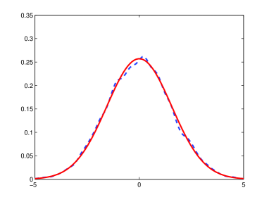
Figure 1: Comparaison of the approximate density $\hat{f}_{h}$ of ${\cal E}_{N}$ (dotted line) with the density of ${\cal N}(0,\bar{\sigma}_{F}^{2})$, $N=5.10^{5}$, $M=5.10^{3}$, $h=M^{-\frac{1}{5}}$.

As a conclusion, this numerical experiment first illustrates that the $CLT$ occurs at a reasonable range (for numerical purpose) and also suggests that a local version holds true as well (“convergence of the density”). Another extension of our result could be, in the spirit of Bhattacharia’s result in [4] to establish an invariance principle of Donsker type.

Appendix

A. Proof of identity (2.19).

We have to deduce (2.19) from (2.16). First, we have (dropping ^x in $A^{x}_{t}$):

$$\mathbb{E}_{\nu}\left[\left(\mathbb{E}[A_{{}_{2T}}|{\cal F}_{{}_{2T}}]-\int_{T}^{2T}\sigma^{*}\nabla g_{{}_{F}}(X_{u}^{x})dW_{u}\right)\mathbb{E}[A_{{}_{T}}|{\cal F}_{{}_{T}}]\right] =\mathbb{E}_{\nu}\left[\mathbb{E}[A_{{}_{2T}}|{\cal F}_{{}_{2T}}]\mathbb{E}[A_{{}_{T}}|{\cal F}_{{}_{T}}]\right]$$

$$=\mathbb{E}_{\nu}[(\mathbb{E}[A_{{}_{T}}|{\cal F}_{{}_{T}}])^{2}]$$

since one easily checks that $\mathbb{E}[A_{{}_{2T}}-A_{{}_{T}}|{\cal F}_{{}_{T}}]=0$. It follows that

$$T\sigma^{2}_{{}_{F}}=\mathbb{E}_{\nu}\left[\left(\mathbb{E}[A_{{}_{2T}}|{\cal F}_{{}_{2T}}]-\int_{T}^{2T}\sigma^{*}\nabla g_{F}(X_{u})dW_{u}\right)^{2}\right]-\mathbb{E}_{\nu}[(\mathbb{E}[A_{{}_{T}}|{\cal F}_{{}_{T}}])^{2}].$$

Second, using the Markov property (or the fact that $X^{(u),x}=\varphi(X_{u}^{x},W^{(u)})$) and the stationarity of the process, one observes that $\mathbb{E}[A_{{}_{2T}}-A_{{}_{T}}|{\cal F}_{{}_{2T}}]$ and $\mathbb{E}[A_{{}_{T}}|{\cal F}_{{}_{T}}]$ have the same distribution under $\mathbb{P}_{\nu}$. In particular,

$$\mathbb{E}_{\nu}\left[\left(\mathbb{E}[A_{{}_{2T}}-A_{{}_{T}}|{\cal F}_{{}_{2T}}]\right)^{2}\right]=\mathbb{E}_{\nu}\left[\left(\mathbb{E}[A_{{}_{T}}|{\cal F}_{{}_{T}}]\right)^{2}\right].$$

Since $\mathbb{E}[A_{{}_{2T}}|{\cal F}_{{}_{2T}}]=A_{{}_{T}}+\mathbb{E}[A_{{}_{2T}}-A_{{}_{T}}|{\cal F}_{{}_{2T}}]$ and $\mathbb{E}_{\nu}[A_{{}_{T}}\mathbb{E}[A_{{}_{2T}}-A_{{}_{T}}|{\cal F}_{{}_{2T}}]]=0$, we obtain that

$$T\sigma^{2}_{{}_{F}}=\mathbb{E}_{\nu}[A_{{}_{T}}^{2}]-2\mathbb{E}_{\nu}\left[\mathbb{E}[A_{{}_{2T}}|{\cal F}_{{}_{2T}}]\int_{T}^{2T}\sigma^{*}\nabla g_{{}_{F}}(X_{u})dW_{u}\right]+\mathbb{E}_{\nu}\left[\left(\int_{T}^{2T}\sigma^{*}\nabla g_{{}_{F}}(X_{u})dW_{u}\right)^{2}\right].$$

All we have to do now is to check that the three above terms correspond respectively to the three parts of (2.19). First, by Fubini’s Theorem,

$$\mathbb{E}_{\nu}[A_{{}_{T}}^{2}]=\int_{u=0}^{T}\int_{v=0}^{T}\mathbb{E}_{\nu}[(F(X^{(u)}-f_{{}_{F}}(X_{u}))(F(X^{(v)}-f_{{}_{F}}(X_{v})))]dv.$$

Owing to the stationarity of the process under $\mathbb{P}_{\nu}$, we have

$$\mathbb{E}_{\nu}[(F(X^{(u)}-f_{{}_{F}}(X_{u}))(F(X^{(v)}-f_{{}_{F}}(X_{v})))]=C_{{}_{F}}(|u-v|),$$

where $C_{{}_{F}}$ is defined by (2.20). This yields

$$\mathbb{E}_{\nu}[A_{{}_{T}}^{2}]=2\int_{0}^{T}\int_{0}^{u}C_{{}_{F}}(u-v)dvdu=2\int_{0}^{T}(T-u)C_{{}_{F}}(u)du.$$

Second, setting

$$M_{T}^{f}=\int_{0}^{t}\sigma^{*}\nabla f(X_{u})dW_{u},$$ (7.65)

we have

$$\mathbb{E}_{\nu}\left[\mathbb{E}[A_{{}_{2T}}|{\cal F}_{{}_{2T}}]\int_{T}^{2T}\sigma^{*}\nabla g_{{}_{F}}(X_{u})dW_{u}\right]= \int_{0}^{2T}\mathbb{E}_{\nu}[(F_{{}_{T}}(X^{(u)})-f_{{}_{F}}(X_{u}))(M_{{}_{2T}}^{g_{{}_{F}}}-M_{{}_{T}}^{g_{{}_{F}}})]du$$

$$= \int_{0}^{T}\mathbb{E}_{\nu}[(F_{{}_{T}}(X^{(u)})-f_{{}_{F}}(X_{u}))(M_{{}_{T+u}}^{g_{{}_{F}}}-M_{{}_{T}}^{g_{{}_{F}}})]du$$

$$+\int_{T}^{2T}\mathbb{E}_{\nu}[(F_{{}_{T}}(X^{(u)})-f_{{}_{F}}(X_{u}))(M_{{}_{2T}}^{g_{{}_{F}}}-M_{{}_{u}}^{g_{{}_{F}}})]du.$$

Now, the fact that $M_{{}_{T+u}}^{g_{{}_{F}}}-M_{{}_{T}}^{g_{{}_{F}}}=g_{{}_{F}}(X_{T+u})-g_{{}_{F}}(X_{T})-\int_{T}^{T+u}{\cal A}g_{F}(X_{v})dv$ implies that we can make use of the stationarity property to obtain for every $u\in[0,T]$,

$$\mathbb{E}_{\nu}[(F_{{}_{T}}(X^{(u)})-f_{{}_{F}}(X_{u})) (M_{{}_{T+u}}^{g_{{}_{F}}}-M_{{}_{T}}^{g_{{}_{F}}})]$$

$$=\mathbb{E}_{\nu}\left[\left(F_{{}_{T}}(X)-f_{{}_{F}}(X_{0})\right)\left(g_{{}_{F}}(X_{T})-g_{{}_{F}}(X_{0})-\int_{0}^{T}{\cal A}g_{F}(X_{v})dv\right)\right]$$

$$=\mathbb{E}_{\nu}[(F_{{}_{T}}(X)-f_{{}_{F}}(X_{0}))(M_{T}^{g_{{}_{F}}}-M_{T-u}^{g_{{}_{F}}})].$$

With similar arguments, one checks that for every $u\in[T,2T]$,

$$\mathbb{E}_{\nu}[(F_{{}_{T}}(X^{(u)})-f_{{}_{F}}(X_{u}))(M_{{}_{2T}}^{g_{{}_{F}}}-M_{{}_{u}}^{g_{{}_{F}}})]=\mathbb{E}_{\nu}[(F_{{}_{T}}(X)-f_{{}_{F}}(X_{0}))M_{{}_{2T-u}}^{g_{{}_{F}}}].$$

It follows that

$$\mathbb{E}_{\nu}\left[\mathbb{E}[A_{{}_{2T}}|{\cal F}_{{}_{2T}}]\int_{T}^{2T}\sigma^{*}\nabla g_{{}_{F}}(X_{u})dW_{u}\right]$$

$$=\mathbb{E}_{\nu}\left[\left(F_{{}_{T}}(X)-f_{{}_{F}}(X_{0})\right)\left(TM_{T}^{g_{{}_{F}}}-\int_{0}^{T}M_{T-u}^{g_{{}_{F}}}du+\int_{T}^{2T}M_{{}_{2T-u}}^{g_{{}_{F}}}du\right)\right]=T\mathbb{E}_{\nu}[F_{{}_{T}}(X)M_{T}^{g_{{}_{F}}}].$$

$$\mbox{Finally, }\qquad\mathbb{E}_{\nu}\left[\left(\int_{T}^{2T}\sigma^{*}\nabla g_{{}_{F}}(X_{u})dW_{u}\right)^{2}\right] =\int_{T}^{2T}\mathbb{E}_{\nu}\left[\left|\sigma^{*}\nabla g_{F}(X_{u})\right|^{2}\right]du\qquad\qquad\qquad$$

$$=T\int|\sigma^{*}\nabla g_{F}(x)|^{2}\nu(dx)$$

owing to the stationarity of the process. This concludes the proof. $\Box$

B. Computation of $\sigma^{2}_{{}_{F}}$ when $F(\alpha)=\phi(\alpha_{{}_{T}})$.

As mentioned in (2.3), when $\phi={\cal A}h+C$, the $CLT$ for marginal functions combined with a change of variable yields $\sigma^{2}_{{}_{F}}=\int_{\mathbb{R}^{d}}|\sigma^{*}\nabla h(x)|^{2}\nu(dx)$. Let us check this formula starting from (2.16). Following the notation introduced in (7.65), we have

$$\mathbb{E}[A_{{}_{2T}}|{\cal F}_{{}_{2T}}]-\mathbb{E}[A_{{}_{T}}|{\cal F}_{{}_{T}}]-\int_{T}^{2T}\sigma^{*}\nabla g_{{}_{F}}(X_{u}^{x})dW_{u}=\varphi_{1}(x,.)-\varphi_{2}(x,.)\quad\textnormal{where,}$$

$$\varphi_{1}(x,.)=\int_{0}^{T}\phi(X_{u+T}^{x})du+\int_{T}^{2T}\mathbb{E}\left[\phi(X_{u+T}^{x}){\cal F}_{2T}\right]du-\int_{T}^{2T}f_{{}_{F}}(X_{u}^{x})du-(M_{2T}^{g_{{}_{F}}}-M_{T}^{g_{{}_{F}}})\quad\textnormal{and}$$

$$\varphi_{2}(x,.)=\int_{0}^{T}\mathbb{E}\left[\phi(X_{u+T}^{x})\,|\,{\cal F}_{T}\right]du.$$

In this case, $f_{{}_{F}}=P_{{}_{T}}\phi$ and using that ${\cal A}$ and $P_{{}_{T}}$ commute, one checks that $f_{{}_{F}}-\nu(f_{{}_{F}})={\cal A}P_{{}_{T}}h$. This implies that $g_{{}_{F}}=P_{{}_{T}}\phi$. For the sake of simplicity we may assume w.l.g. $\nu(f_{{}_{F}})=\nu(\phi)=0$. Then, on the one hand

$$\varphi_{1}(x,.) = \int_{T}^{2T}{\cal A}h(X_{u})du+\int_{T}^{2T}P_{u-T}\phi(X_{2T})du-\Big{[}g_{{}_{F}}(X_{2T})-g_{{}_{F}}(X_{{}_{T}})\Big{]}$$

$$= h(X_{2T})-h(X_{T})-(M_{2T}^{h}-M_{T}^{h})+\int_{0}^{T}{\cal A}P_{u}h(X_{2T})du-\Big{[}g_{{}_{F}}(X_{2T})-g_{{}_{F}}(X_{{}_{T}})\Big{]}$$

$$= h(X_{2T})-h(X_{T})-(M_{2T}^{h}-M_{T}^{h})+\underbrace{P_{{}_{T}}h(X_{2T})}_{=g_{{}_{F}}(X_{2T})}-h(X_{2T})-\Big{[}g_{{}_{F}}(X_{2T})-g_{{}_{F}}(X_{{}_{T}})\Big{]}$$

$$= g_{{}_{F}}(X_{T})-h(X_{T})-(M_{2T}^{h}-M_{T}^{h}).$$

On the other hand

$$\varphi_{2}(x,.)=\int_{0}^{T}P_{u}\phi(X_{T})du=\int_{0}^{T}{\cal A}P_{u}h(X_{T})du=P_{{}_{T}}h(X_{T})-h(X_{T})=g_{{}_{F}}(X_{T})-h(X_{T}).\\$$

so that

$$\sigma^{2}_{{}_{F}}=\frac{1}{T}\mathbb{E}_{\nu}[(M_{2T}^{h}-M_{T}^{h})^{2}]=\frac{1}{T}\int_{T}^{2T}\mathbb{E}_{\nu}[|\sigma^{*}\nabla h(X_{u})|^{2}]du=\int|\sigma^{*}\nabla h(x)|^{2}\nu(dx).\qquad\Box$$

References

• [1] Alfonsi A. (2005). On the discretization schemes for the CIR (and Bessel squared) processes, Monte Carlo Methods Appl, 11, 355–384. 2186814
• [2] Andersen, Leif B. G., Efficient Simulation of the Heston Stochastic Volatility Model (January 23, 2007). Available at SSRN: http://ssrn.com/abstract=946405
• [3] Basak G.K., Bhattacharya R.N. (1992). Stability in Distribution for a Class of Singular Diffusions, Ann. Probab., 20(1):312–321.
• [4] Bhattacharya R.N. (1982). On the functional Central Limit Theorem and the law of the iterated logarithm for Markov processes, Z. Wahrsch. Verw. Gebiete., 60(2):185–201.
• [5] Berkaoui A., Bossy M., Diop A. (2008). Euler scheme for SDE’s with non-Lipschitz diffusion coefficient: strong convergence, ESAIM Probab. Stat., 12, 1–11. 2367990
• [6] Billingsley P. (1968) Convergence of Probability Measures, Wiley. 02333096
• [7] Bouleau N., Lépingle D. (1994). Numerical methods for stochastic processes, John Wiley & Sons, Inc., New York, 359 p. 1274043
• [8] Deelstra G., Delbaen F. (1998). Convergence of Discretized Stochastic (Interest Rate) Processes with Stochastic Drift Term, Appl. Stochastic Models Data Anal., 14, 77-84. 1641781
• [9] Duflo M. (1997). Random Iterative Models, Springer Verlag, Berlin. 1485774
• [10] Hall P., Heyde C. (1980). Martingale Limit Theory and its Application, Academic Press.
• [11] Heston S. (1993). A closed-form solution for options with stochastic volatility with applications to bond and currency options, Review of Financial Studies, 6:327-343.
• [12] Jacod J., Shiryaev A. N. (1987). Limit Theorems for Stochastic Processes, Springer. 1943877
• [13] Karatzas I., Shreve S. (1991), Brownian Motion and Stochastic Calculus, Springer. 1121940
• [14] Kloeden P., Platen E. (1992) Numerical solution of stochastic differential equations. Applications of Mathematics (New York), 23. Springer-Verlag, Berlin, 1992. 632 pp. 3-540-54062-8
• [15] Kunita H. (1982). Stochastic differential equations and stochastic flows of diffeomorphisms. Cours d’école d’été de Saint-Flour, LN-1097, Springer-Verlag, 1982.
• [16] Ladyzhenskaya, O. A., Ural’tseva, N. N. (1968). Linear and quasilinear elliptic equations. Academic Press, New York-London:495 p. 244627
• [17] Lamberton D. and Lapeyre B. (1996). Introduction to Stochastic Calculus Applied to Finance, Chapman and Hall/CRC, New York. 1422250
• [18] Lamberton D. and Pagès G. (2002). Recursive computation of the invariant distribution of a diffusion. Bernoulli 8:367-405. 1913112
• [19] Lamberton D. and Pagès G. (2003). Recursive computation of the invariant distribution of a diffusion: The case of a weakly mean reverting drift. Stoch. Dynamics 4:435-451. 2030742
• [20] Lemaire V. (2007). An adaptive scheme for the approximation of dissipative systems. Stochastic Process. Appl. 117:1491-1518. 2353037
• [21] Lemaire V. (2005). Estimation numérique de la mesure invariante d’un processus de diffusion, PhD Thesis, Université de Marne-La Vallée.
• [22] Pagès G., Panloup F. (2009). Approximation of the distribution of a stationary Markov process with application to option pricing. Bernoulli, 15(1):146–177. 2546802
• [23] Panloup F. (2008). Recursive computation of the invariant measure of a SDE driven by a Lévy process. Ann. Appl. Probab. 18:379-426. 2398761
• [24] Panloup F. (2008). Computation of the invariant measure of a Lévy driven SDE: Rate of convergence, Stochastic Process. Appl., 118(8):1351–1384. 2427043
• [25] Panloup F. (2006). Approximation du régime stationnaire d’une EDS avec sauts, PhD Thesis, Université Paris VI.
• [26] Pardoux E., Veretennikov A. (2001). On Poisson equation and diffusion approximation I, Ann. Probab., 29(3):1061–1085. 1872736
• [27] Pardoux E., Veretennikov A. (2003). On Poisson equation and diffusion appoximation II, Ann. Probab, 31(3):1166–1192. 1988467
• [28] Pardoux E., Veretennikov A. (2006). On the Poisson equation and diffusion approximation III, Ann. Probab, 33(3):1111–1133. 2135314
• [29] Protter P. (2005) Stochastic integration and differential equations. Second edition. Version 2.1. Corrected third printing. Stochastic Modelling and Applied Probability, 21. Springer-Verlag, Berlin:419 pp. 3-540-00313-4
• [30] Talay D. (1990). Second order discretization schemes of stochastic differential systems for the computation of the invariant law. Stoch. Stoch. Rep., 29(1):13-36.