Group finding in the stellar halo using M-giants in 2MASS: An extended view of the Pisces Overdensity?

Abstract

A density based hierarchical group-finding algorithm is used to identify stellar halo structures in a catalog of M-giants from the Two Micron All Sky Survey (2MASS). The intrinsic brightness of M-giant stars means that this catalog probes deep into the halo where substructures are expected to be abundant and easy to detect. Our analysis reveals 16 structures at high Galactic latitude (greater than $15^{\circ}$), of which 10 have been previously identified. Among the six new structures two could plausibly be due to masks applied to the data, one is associated with a strong extinction region and one is probably a part of the Monoceros ring. Another one originates at low latitudes, suggesting some contamination from disk stars, but also shows protrusions extending to high latitudes, implying that it could be a real feature in the stellar halo. The last remaining structure is free from the defects discussed above and hence is very likely a satellite remnant. Although the extinction in the direction of the structure is very low, the structure does match a low temperature feature in the dust maps. While this casts some doubt on its origin, the low temperature feature could plausibly be due to real dust in the structure itself. The angular position and distance of this structure encompass the Pisces overdensity traced by RR Lyraes in Stripe 82 of the Sloan Digital Sky Survey (SDSS). However, the 2MASS M-giants indicate that the structure is much more extended than what is visible with the SDSS, with the point of peak density lying just outside Stripe 82. The morphology of the structure is more like a cloud than a stream and reminiscent of that seen in simulations of satellites disrupting along highly eccentric orbits. This finding is consistent with expectations of structure formation within the currently favored cosmological model: assuming the cosmologically-predicted satellite orbit distributions are correct, prior work indicates that such clouds should be the dominant debris structures at large Galactocentric radii ($\sim 100$ kpc and beyond).

1. Introduction

Under the currently favored $\Lambda$CDM model of galaxy formation, the stellar halo is thought to have been built up, at least in part, hierarchically through mergers of smaller satellite systems. Signatures of these mergers should be apparent as structures in the stellar halo (Johnston, 1998; Helmi & White, 1999; Bullock et al., 2001; Johnston et al., 2008). In recent years observations have lent support to the hierarchical picture with the discovery of a number of streams and structures of stars in the stellar halo of the Milky Way. The most prominent of these structures are the tidal tails of the Sagittarius dwarf galaxy (Ibata et al., 1994, 1995; Majewski et al., 2003), the Virgo overdensity (Jurić et al., 2008), the Triangulum-Andromeda structure (Rocha-Pinto et al., 2004; Majewski et al., 2004; Martin et al., 2007) and the low latitude Monoceros ring (Newberg et al., 2002; Yanny et al., 2003; Peñarrubia et al., 2005; Martin et al., 2005).

The mapping of these low surface brightness structures can be attributed to the advent of large scale stellar catalogs derived from surveys such as the Two Micron All Sky Survey (2MASS) and the Sloan Digital Sky Survey (SDSS). Typically, a judicious color selection is applied to objects in a survey in order to maximise the presence of stars with some well-defined absolute magnitude range. Structures are then identified by visually inspecting sky-projections of the stellar density in slices of apparent magnitude. Future surveys, such as GAIA (Perryman, 2002), LSST (Ivezic et al., 2009) SkyMapper (Keller et al., 2007) and PanSTARRS, will explore the stellar halo to greater depth, with even larger numbers of stars and in more dimensions and should be sensitive to even more structures.

While discovery by visual inspection has proved successful so far, the scale and sophistication of the maps generated from these data sets (both current and future) motivate an exploration of methods that can instead objectively identify structures. This task is well suited to clustering algorithms, which have enjoyed great success in other areas of astronomy, e.g., identifying galaxy groups in redshift surveys (Eke et al., 2004) or identifying halos in cosmological simulations (Reed et al., 2007; Jenkins et al., 2001; Lacey & Cole, 1993). The stellar halo presents unique challenges for such algorithms. The structures in the stellar halo have arbitrary shapes, they span a wide range of densities that cannot be separated by a single isodensity contour and they can have nested substructures. In this paper we present an objective analysis of substructures in the stellar halo using the code EnLink (Sharma & Johnston, 2009), which is a density-based hierarchical group finder. The code is ideally suited for this application for four reasons. First, a density-based group-finder is able to identify irregular groups. Second, EnLink’s clustering scheme can identify groups at all density levels. Third, EnLink’s organizational scheme allows the detection of the full hierarchy of structures. Finally, the group finder gives an estimate of the significance of the groups, so spurious clusters can be ignored.

Among the existing surveys, the 2MASS catalog of M-giant stars and the SDSS catalog of F and G type main-sequence-turnoff (MSTO) stars provide the clearest global views of the stellar halo. While SDSS contains a larger number of stars than 2MASS M-giants, it covers only about 10,000 ${\rm deg}^{2}$ (1/4 of the sky) in area. Moreover, the magnitude limit of SDSS means that MSTO stars can probe the stellar halo only out to 35 $\>{\rm kpc}$ (Bell et al., 2008) while M-giant stars in 2MASS probe out to 100 $\>{\rm kpc}$ (Majewski et al., 2003). This implies that the M-giant stars in 2MASS not only cover a factor of about 90 in volume more than the MSTO stars in SDSS, but also probe the outer halo where the substructures are expected to be more abundant and have higher density contrast. Hence, we choose to apply EnLink to the 2MASS M-giant sample with the aim of objectively identifying substructures within it.

Note that using M-giants as tracers also has its share of disadvantages. First, M-giants are a rare population so the total size of the survey is much smaller than the SDSS MSTO sample. Second, M-giants are metal rich, intermediate-age stars with metallicity [Fe/H] typically greater than $>-1.5$. Hence, applying a group finder to an M-giant survey will preferentially detect high metallicity debris from the few massive recently-accreted objects and will be insensitive to ancient or low-metallicity debris that originates from the many more low mass progenitors. The advantage of this bias against ancient or low-metallicity stars is that it will increase the sensitivity to the rare, recent, high-mass events. However, building a census of debris from all types of accreting objects would require combining these results with those from other surveys—to be discussed in detail in a forthcoming paper (S. Sharma et al. 2010, in preparation).

The paper is organized as follows: Section 2 describes the 2MASS M-giant data set used in the paper; Section 3 discusses the methods employed for analyzing the data, i.e., group finding; in Section 4 we describe the structures identified by the group-finder in the 2MASS M-giant sample; and finally, we summarize our findings in Section 5.

2. Selecting M-giant halo stars from the 2MASS data

The 2MASS all sky point source catalog contains about $471$ million objects (the majority of which are stars) with precise astrometric positions on the sky and photometry in three bands $J,H,$ and $K_{s}$. The survey catalog is $99\%$ complete for $K_{s}<14.3$. An initial sample of candidate M-giants was generated by applying the selection criteria:

$$K_{s} < 14.0$$ (1)

$$J-K_{s} > 0.85$$ (2)

$$J-H < 0.561(J-K_{s})+0.36$$ (3)

$$J-H > 0.561(J-K_{s})+0.19.$$ (4)

All magnitudes in the above equations are in the intrinsic, dereddened 2MASS system (labeled with subscript 0 hereafter), with dereddening applied using the Schlegel et al. (1998) extinction maps. These selection criteria and the dereddening method are similar to those used by Majewski et al. (2003) to identify the tidal tails of Sagittarius dwarf galaxy. In general, for $(J-K_{s})_{0}>0.85$ giants begin to separate from dwarfs in the near-infrared color-color diagram, with redder colors leading to better discrimination. However, the number density of giants in the catalog falls off rapidly as a function of color. As a compromise between quality (i.e., the level of contamination by disk dwarfs) and quantity we restrict our search to stars with $(J-K_{s})_{0}>0.97$. This generates a list of about $450,000$ stars spanning a magnitude range of $4.12-14.0$ in the $(K_{s})_{0}$ band.

Since we are interested in the stellar halo, we further refine our selection with geometrical factors aimed at reducing contamination by foreground disk stars, as well as adopting masks to cover regions of high dust extinction. First, we impose the twin requirements that $(K_{s})_{0}>10$ and $(K_{s})_{0}{\rm sin}(b)>14.0{\rm sin}(15^{\circ})$. The former condition gets rid of stars near the Sun, while the latter limits the contribution by stars that are further away, but lie close to the Galactic plane. At low latitudes the distribution of stars is not contiguous owing to the presence of extinction clouds, which in some regions extend to a latitude of $30^{\circ}$. To avoid identifying spurious structures and at the same time retain as much low latitude data as possible we mask the high extinction regions by means of a set of rectangles in $(l,b)$ space, as shown in LABEL:f1. Finally, there are some extinction holes in the region of the Large Magellanic Cloud (LMC). We fill these up by identifying the stars lying within a region defined by $\sqrt{(l-280^{\circ}.0)^{2}+(b+33^{\circ}.0)^{2}}<10^{\circ}$ and adding a dispersion of $1^{\circ}$ to their original latitude and longitude coordinates, as illustrated in the left and right panels of LABEL:f2. After applying all of the selection criteria, the final sample contains $59,392$ stars. An Aitoff plot of these M-giants is shown in LABEL:f3.

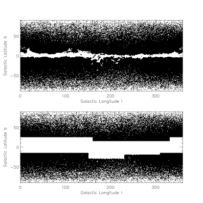
Figure 1.— Latitude vs. longitude scatter plot of M-giant stars identified in the 2MASS data. Top: original data containing extinction regions at low latitudes. Bottom: distribution of stars after masking the extinction regions by means of rectangular patches and retaining stars with latitude $b>15^{\circ}$.

A particularly useful property of M-giants is that their absolute magnitude varies approximately linearly with their color and can be expressed as

$$M_{K_{s}}=A+B(J-K_{s})$$ (5)

A slope of $B=-9.42$ was found to be a good fit, in the regime $0.97<(J-K_{s})_{0}<1.2$, to a range of theoretical isochrones with [Fe/H]$>-1$ and age in range $6-13$ Gyr. The intercept $A$ however depends upon the age and metallicity. Since we do not know the age and metallicity we choose to adopt a constant value of $A=3.26$ that roughly bisects the distribution of $M_{K_{s}}$ versus $(J-K_{s})_{0}$ in the simulated stellar halos of Bullock & Johnston (2005) . One such halo is shown in LABEL:f4 . The dashed lines with $A=3.26\pm 1.1$ represent the range of scatter about this relationship. A detailed discussion of the impact of our assumption of a constant age and metallicity for detecting structures is given Section 3.3.

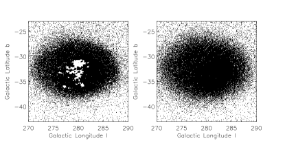
Figure 2.— Latitude vs. longitude scatter plot of M-giant stars in the LMC region. Left: original data showing extinction regions. Right: the same region after adding a dispersion of $1^{\circ}$ to stars satisfying $\sqrt{(l-280^{\circ}.0)^{2}+(b+33^{\circ}.0)^{2}}<10^{\circ}$.

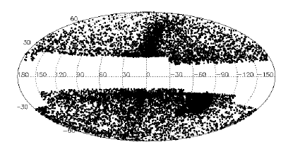
Figure 3.— An Aitoff plot in galactic coordinates of the final 2MASS M-giant catalog that is used for the group-finding analysis.

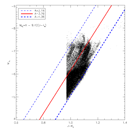
Figure 4.— Absolute magnitude of M-giants as a function of its color in a $K_{s}<14$ volume limited sample of Bullock & Johnston (2005) simulated stellar halo (halo-2). The relationship is well represented by a function of the form $M_{K_{s}}=A-9.42(J-K_{s})$. The solid line with a value of $A=3.26$ is found to roughly bisect the distribution of points in the plot. The dashed lines with $A=3.26\pm 1.1$ represent the range of scatter about this relationship.

3. Methods

3.1. Group finding

In this paper we use the density-based hierarchical group-finder EnLink (described in detail in Sharma & Johnston, 2009) that can cluster a set of data points defined over an arbitrary space. For our application the stars are treated as the data points and the coordinates of the data points are defined by the position of the stars in three-dimensional space. The group finding scheme of EnLink is similar to ISODEN (Pfitzner et al., 1997) and SUBFIND (Springel et al., 2001) and is based on the fact that a system having more than one group will have peaks and valleys in the density distribution, the peaks being formed at the center of the groups and the valleys or saddle points where they overlap. The peaks are identified as groups and the region around each peak, which is bounded by an isodensity contour corresponding to the density at the valley, is associated with the group. This is shown schematically in LABEL:f5 for a one-dimensional case. The valleys also define connections between groups and these are used to assign a parent/child relationship between the groups, resulting in a hierarchy of clusters.

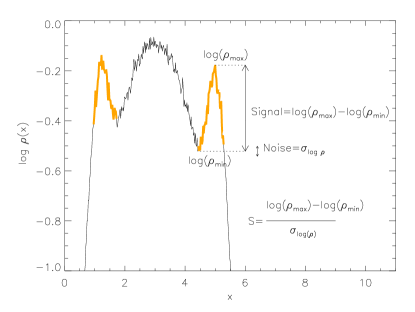
Figure 5.— Schematic illustration of the group-finding scheme in one dimension. The plot shows the distribution of density in space for three superposed Gaussian distributions along with a noise of 0.02 dex. The substructures that are bounded by a valley are represented by the thick light gray (orange) curve. The maximum and minimum values of the density in a group are used to calculate its significance.

To implement the above scheme EnLink first calculates the density using a nearest neighbor scheme, where the number of nearest neighbors $k_{\rm den}$ is fixed and is supplied by the user. A list of $k_{\rm link}=10$ nearest neighbors for each data point is also computed and stored. Next, the points are sorted according to their density in descending order and stored in a list. Starting from the densest, each point from this sorted list is chosen successively and acted upon according to three options:

1. If the point does not have a neighbor denser than itself a cluster is created and the particle is added to it;

2. If its denser neighbors belong to a unique cluster the particle is also added to it;

3. If the denser neighbors belong to different clusters, the two nearest clusters are selected and the point is added to the cluster having the closest neighbor. Also, the smaller of the two nearest clusters becomes a sub-cluster of the larger (now the “parent” cluster) and all future particles that need to be added to the smaller cluster are added to the parent from then on—a process known as sub-cluster attachment.

EnLink employs an additional strategy to screen out spurious groups that can arise due to Poisson noise in the data. EnLink defines the significance $S$ for a group as a ratio of signal associated with a group to the noise in the measurement of this signal (see Figure 5 for a schematic illustration). The contrast $\ln(\rho_{\rm max})-\ln(\rho_{\rm min})$ between the peak density of a group ($\rho_{\rm max}$) and valley ($\rho_{\rm min}$) where it overlaps with another group can be thought of as the signal, and the noise in this signal is given by the variance $\sigma_{\ln(\rho)}$ associated with the density estimator. Combining the definitions of signal and noise then leads to

$$S=\frac{\ln(\rho_{\rm max})-\ln(\rho_{\rm min})}{\sigma_{\ln\rho}}.$$ (6)

For Poisson-sampled data the distribution of density as estimated by the code using the kernel scheme is log-normal and the variance satisfies the relation $\sigma_{\ln(\rho)}=\sqrt{V_{d}||W||_{2}^{2}/k_{\rm den}}$, where $k_{\rm den}$ is the number of neighbors employed for density estimation, $V_{d}$ the volume of a $d$-dimensional unit hypersphere and $||W||_{2}^{2}$ the $L2$ norm of the kernel function (Sharma & Johnston, 2009). For our case, $d=3$ and $k_{\rm den}=30$ and the variance is $\sigma_{\ln(\rho)}=0.22$.

The distribution of the significance parameter $S$ is close to a Gaussian function for Poisson-sampled data. This implies that spurious groups in general have low $S$ and their probability of occurrence falls off like a Gaussian distribution with increasing $S$. Hence, selecting groups using a simple threshold in the significance $S_{\rm Th}$ can get rid of the spurious groups. EnLink uses this recipe to calculate the significance of the groups. All groups below $S_{\rm Th}$ are denied the status of a group and are merged with their respective parent groups.

3.2. Parameter Choices

The number and properties of groups recovered by our clustering algorithm depend in part on the parameters adopted for the group finder itself, as well as how the data are transformed from observable to real-space. In this section, we first define measures to evaluate the performance of our clustering scheme (Section 3.2.1) and subsequently use these measures to guide our choice of data transformation (Section 3.2.2) and group-finding parameters (Section 3.2.3).

3.2.1 Evaluation of clustering

Let $Q$ be a set of data points with two partitions $I$ and $J$, $I$ being the set of intrinsic classes that are known a priori and $J$ being the set of groups or clusters found by the group finder. In our case the data points are the stars in the halo and the intrinsic classes are the individual satellite systems that make up the halo. Overlaps between the two partitions are given by the contingency matrix $n_{ij}$, which gives the number of data points common to both class $i\in I$ and group $j\in J$. The class that is most frequent (${\rm argmax}_{i\in I}n_{ij}$) in a group is the class discovered by the group, and $D_{i}$ is the set of all groups in which class $i$ is discovered.

One measure of success for our group finder is the degree to which recovered groups represent intrinsic classes, which in our case correspond to real physical associations. We therefore define purity as the fraction of correctly classified points in a group $j$ :

$${\rm Purity}(j) = \frac{{\rm max}_{i\in I}\{n_{ij}\}}{n_{.j}},$$ (7)

where $n_{.j}=\sum_{i}n_{ij}$ is the total number of data points in that group. The mean value of purity $P=\sum{\rm Purity}(j)/|J|$ is then a good indicator of the overall quality of the clustering.

We would also like to know how much of an intrinsic class can typically be recovered—in our case this corresponds to reconstructing long-dead satellites. In clustering algorithms, the fraction of correctly classified points in a class summed over all groups where the class is discovered is traditionally known as the recall of a class. We modify this definition slightly to also take into account the purity of the discovered points and define penalized recall as

$${\rm PRecall}(i) = \sum_{j\in D_{i}}\frac{n_{ij}}{n_{i.}}({\rm Purity}(j)-0.5)2,$$ (8)

where $n_{i.}=\sum_{j}n_{ij}$ is the total number of data points in class $i$. The total value of penalized recall, $\sum{\rm PRecall}(i)$, represents the mean number of classes discovered by the group finder along with a penalty term for classes discovered with purity less than 0.5. This is a good indicator of the overall amount of clustering.

While mean purity and total penalized recall are sensitive to different aspects of clustering, in many situations they vary inversely with each other and hence both of them should be taken into account when evaluating clustering success. We do this by defining a clustering performance index (CPI), which is given by

$${\rm CPI} = \sum_{i}{\rm PRecall}(i)\frac{\sum_{j}{\rm Purity}(j)}{|J|}.$$ (9)

The larger the value of ${\rm CPI}$ the better are the clustering results. Typically the value of ${\rm CPI}$ ranges between 0 and $|I|$. The maximum value occurs when both the mean purity and total recall have their maximum values, which are 1 and $|I|$ respectively. In some extreme circumstances, e.g., when the total recall is negative, CPI can be negative and the minimum possible value is –$|I|$.

3.2.2 Choice of coordinate system and metric

The efficiency of detecting structures in a data set depends upon the choice of the coordinate system in which the data are described and the metric (a function of coordinates that defines the distance between any two points in a space) used to calculate distances. The simplest metric is the Euclidean metric—appropriate when all the dimensions are of the same physical units, such as the Cartesian coordinate system defined by the $x,y,z$ position of stars in a three-dimensional space. The observational data of stars, however, are in a spherical coordinate system given by the two angular positions on the sky and the radial distance. If the uncertainty associated with the coordinates is small, the data can be easily converted to the Cartesian system. More realistically, the angular coordinates can be directly measured with very high precision but the radial distance needs to be estimated indirectly from the properties of the stars and hence has large uncertainty associated with it. For example, as discussed in Majewski et al. (2003) we expect a distance uncertainty of about 18% for the M-giants in our sample, and in this case using the simple Cartesian coordinate system could severely degrade the quality of clustering.

A common solution in cases having large uncertainty in one of the coordinates is to perform a dimensionality reduction and analyze the data in a lower dimensional space—for example, in our case using angular positions alone. An alternative to ignoring the radial dimension altogether is to redefine the radial coordinate in a logarithmic scale and then use this modified radial coordinate to convert the data to a Cartesian system. The advantage of this transformation lies in the fact that while the dispersion in radial distance $r$ increases linearly with $r$, the dispersion in modified radial coordinate $\log(r)$ is constant. This motivates a transformation of our radial coordinate to $r^{\prime}=5(\log(r/(10{\rm pc})))-\mu_{0}$ where $\mu_{0}$ is a constant that determines the degree to which the radial dimension is ignored or used. If $\mu_{0}$ is small the data lie in a thin shell, which is equivalent to ignoring the radial dimension altogether. On the other hand, if $\mu_{0}$ is large the radial dimension is given more prominence.

In order to demonstrate the effectiveness of our coordinate transformation we applied the group-finder EnLink (with parameters $k_{\rm den}=30$ and $S_{\rm Th}=4.25$) to a synthetic stellar halo survey generated from the simulations of Bullock & Johnston (2005). As a particularly stringent test we chose to look at a stellar halo that had been constructed entirely from low-luminosity satellites and hence contained numerous small, low-contrast structures rather than a few large ones (corresponding to the “low-luminosity halo”, amongst the six non $\Lambda$CDM halo models described in Johnston et al., 2008). A color limit of $0.1<g-r<0.3$ and a magnitude limit of $M_{r}<24.5$ (in the SDSS $ugriz$ band) were used to generate the model halo. Two samples were generated from the model, both with and without distance errors—referred to as data $T$ and data $T_{\rm error}$ respectively. The group finder was run in both the normal coordinate system and the modified coordinate system (with $\mu_{0}=8$). For data $T_{\rm error}$ we assumed a distance uncertainty of $\sigma_{r}/r=0.25$. To compare clustering we use two measures: the number of detected groups $G$ and the clustering performance index CPI (defined in Section 3.2.1). The results are tabulated in Table 1. It can be seen that for data without errors the clustering results are similar in both the coordinate systems, but for data with errors, clustering is better in the modified coordinate system as evidenced by the increase in both $G$ and CPI.

Next to choose an appropriate value of $\mu_{0}$ we compared the clustering results, for the data $T_{\rm error}$, in the modified coordinate system with different values of $\mu_{0}$. The CPI was found to be maximum at $\mu_{0}\sim 8$ and hence we adopt this value for rest of our analysis. It should be noted that the clustering results were not strongly sensitive to the exact choice of $\mu_{0}$, in fact CPI was found to vary very little in the range $-10<\mu_{0}<10$. In general, decreasing $\mu_{0}$ was found to increase the number of detected groups. However, the mean purity of groups was found to decrease with $\mu_{0}$, so choosing a value of $\mu_{0}$ too small would mean greater contamination by spurious groups.

Table 1 Comparison of Clustering Performance

Data	Radial Coordinate	$\sigma_{r}/r$	Sample Size	Groups	$CPI$
$T$	$r$	0.0	$2\times 10^{7}$	114	11.1
$T_{\rm error}$	$r$	0.25	$2\times 10^{7}$	15	0.5
$T$	$5\log(r/10{\rm pc})-\mu_{0}$	0.0	$2\times 10^{7}$	118	8.9
$T_{\rm error}$	$5\log(r/10{\rm pc})-\mu_{0}$	0.25	$2\times 10^{7}$	35	2.3
$T^{\prime}_{\rm M-giants}$	$5\log(r/10{\rm pc})-\mu_{0}$	0.15	$2.5\times 10^{4}$	15
$T_{\rm M-giants}$	$5\log(r/10{\rm pc})-\mu_{0}$	Eq-5	$2.5\times 10^{4}$	17

3.2.3 Optimum choice of group-finding parameters

The two free parameters in the group-finder are the number of neighbors employed for density estimation, $k_{\rm den}$, and the significance threshold, $S_{\rm Th}$, of the groups. We select $k_{\rm den}=30$: a smaller value makes the results of the clustering algorithm sensitive to noise in the data, while a larger value means that small structures go undetected.

The choice of the second free parameter, $S_{\rm Th}$, is governed by the desire to make the expected number of spurious groups, which can arise due to Poisson noise in the data, either constant or zero. This is important if one wants to reliably use the number of detected groups as a measure of clustering strength. For a $d$-dimensional data consisting of $N$ points an optimum value of $S_{\rm Th}$ can be chosen by considering the number of spurious groups with significance greater than $S_{\rm Th}$ expected for a Poisson-distributed data (i.e., data points being distributed in a finite region of space uniformly but randomly). The required expression is given by

$$G(>S_{\rm Th})=(1-{\rm erf}(S_{\rm Th}/\sqrt{2}))\frac{15.5N}{d^{2.1}k_{\rm den}^{1.2}}$$ (10)

(Sharma & Johnston, 2009). Since the presence of even one or two spurious groups can severely contaminate the analysis of structures we calculate the optimum value of $S_{\rm Th}$ for a given $N$ by setting the expected number of spurious groups $G(>S_{\rm Th})=0.5$ in equation (10) and solve for $S_{\rm Th}$. Using this method we find $S_{\rm Th}=3.75$ for $N=10^{5}$ (typical size of the data analyzed in this paper). In general, decreasing $S_{\rm Th}$ decreases the number of recovered groups and the value of total recall, but increases the mean purity. On the other hand increasing $S_{\rm Th}$ has exactly the opposite behavior. This suggests that CPI should be maximum at some optimum value of $S_{\rm Th}$. In our tests on synthetic halos we do see this behavior, i.e., for values of $S_{\rm Th}$ for which $G(>S_{\rm Th})=0.5$, CPI also tends to be maximum.

As a final confirmation of our choice of threshold $S_{\rm Th}$, we generated a data set that contained only noise by replacing the latitude and longitude measured for 2MASS M-giant stars with values selected at random from a uniform distribution over a sphere but excluding the low latitude regions (as in the case of the real 2MASS M-giant sample). We then applied the group-finder to this randomized data-set with $S_{\rm Th}=1$. The distribution of significance $S$ for the recovered groups is shown as the dotted histogram in the top panel of LABEL:f6. The groups have a distribution that is like the tail of a Gaussian, with very few groups having $S>3.75$. The distribution of groups recovered from the real 2MASS M-giant sample (solid line) is similar to that for randomized data for $S<3.75$. However, for $S>3.75$ several extra groups can be seen. This suggests that choosing a significance threshold of $S_{\rm Th}=3.75$ to identify groups in a survey containing $10^{5}$ points will minimize contamination by spurious groups.

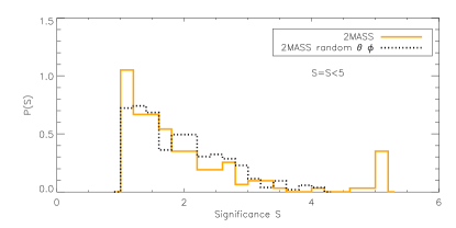
Figure 6.— Distribution of significance $S$ for the groups identified by the group-finder. Groups with $S>5$ were assigned a value of $S=5$. The plot shows the results for the 2MASS M-giant data and a randomized 2MASS M-giant data created by choosing the latitude and longitude at random so as to have a uniform distribution over a sphere.

3.3. Impact of the assumption of a single age and metallicity

In Section 2 we had tentatively assumed a value of $A=3.26$ in the color magnitude relation (represented by Equation (5), referred to as CMR hereafter), which corresponds to assuming a single age and metallicity for all the stars. We now revisit this issue and study the impact of this assumption for group-finding studies.

First, we note that as a consequence of working in a space of modified radial coordinate (see Section 3.2.2), there is a complete degeneracy between the choice of parameters $\mu_{0}$ and $A$. Since our analysis in Section 3.2.2 has already shown that group finding is insensitive to the exact choice of $\mu_{0}$, the same applies for $A$. The relative insensitivity of clustering to $\mu_{0}$ or $A$ is because a change in value of either of them leads to a mere translation of the data in the radial direction while the geometry of structures within the data remains almost intact.

Although the ability to identify structures is not sensitive to the exact choice of $A$, it is sensitive to the scatter of the stars about the adopted CMR (as shown in LABEL:f4). The standard deviation of distance modulus $\sigma_{\mu}$ computed using the adopted CMR for the full halo was found to be 0.51. This high value of $\sigma_{\mu}$ is mostly due to systematic differences in metallicities and ages between satellite system rather than large ranges internal to each system. These systematic differences simply translate the structures relative to each other in space, an effect which does not significantly hamper how well they can be detected. For the purpose of detecting structures what matters most is the $\sigma_{\mu}$ for individual satellite systems. Using the simulated stellar halos of Bullock & Johnston (2005) we found the mean value of $\sigma_{\mu}$ for individual satellite systems to be 0.34, i.e., distance uncertainty $\sigma_{r}/r=0.15$, in accordance with our expectation. These dispersion estimates are also in agreement with the results of Majewski et al. (2003), where they report $\sigma_{\mu}=0.36$ for the 2MASS M-giants in the core of Sagittarius.

Our previous discussion suggests that using the 2MASS M-giants along with our adopted CMR for distance determination should be roughly equivalent to using a data set with about 15% dispersion in distance estimates. To test this we employ the same low luminosity halo that was used in Section 3.2.2 but now generate a sample of M-giants using the color magnitude limits as described in Section 2 for the real 2MASS M-giant data. Equation (10) was used to select the optimum $S_{\rm Th}$ relevant for the present data size and the group finder was run once with $15\%$ errors in distance (data $T^{\prime}_{\rm M-giants}$) and once with distance computed using Equation (5) (data $T_{\rm M-giants}$). The results are tabulated in Table 1. It can be seen that both data sets give nearly the same number of groups which demonstrates that for the purpose of detecting groups, the effect of using a constant age and metallicity is similar to that of data with 15% error in radial distances.

Comparing the number of detected groups in Table 1 for different data sets also allows us to compare the overall group-finding efficiency of different schemes. We find that of the groups that could have been detected without any distance errors (data set $T$), only 30% are detected by data $T_{\rm error}$ and 15% by data $T_{\rm M-giants}$. Although the drop in ability to detect groups is quite dramatic, it is mainly a reflection of the fact that fainter structures that are harder to detect are much more numerous than the brighter and easily detectable structures. Additionally, our results are biased by the fact that we use a hypothetical halo dominated by low mass accretion events which are also the ones that are preferentially missed in a data with measurement errors. Hence, for a realistic $\Lambda$CDM halo we expect the percentage of detected groups to be slightly higher.

Next, we compare the number of detected groups for data $T_{\rm M-giants}$ with data $T_{\rm error}$. Although the distance error for data $T_{\rm M-giants}$ is less than that for data $T_{\rm error}$, the number of detected groups is still about a factor of 2 lower. Three factors could be responsible for this. First, the sample size for $T_{\rm M-giants}$ is three order of magnitude lower than that for data $T_{\rm error}$, which means that the data $T_{\rm M-giants}$ has lower spatial resolution and this makes identification of groups difficult. Second, M-giant data is biased toward detecting high metallicity, intermediate-age stars and would miss low metallicity systems or those accreted long ago, which dominate by number. Finally, the high mass systems, which are preferentially sampled by M-giants due to their high metal content, are also the most phase mixed ones and contribute more to the smooth background, making structure detection even more difficult. In fact, in a forthcoming paper (S. Sharma et al. 2010, in preparation) we demonstrate that, despite the low number of stars, a 2MASS type survey can recover most of the structures that originate from high mass progenitors and are on orbits of low eccentricity.

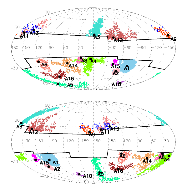
Figure 7.— Groups found in the 2MASS M-giant sample shown in Aitoff projection maps centered at $0^{\circ}$ longitude (upper panel) and $180^{\circ}$ longitude (lower panel). Large black filled circles mark the position of the density peak in a group. Stars in each group are color coded with a unique color and are shown as small filled circles. The solid black lines mark the low latitude area that is excluded from the analysis. Note that group A7 lies on the top of group A2.

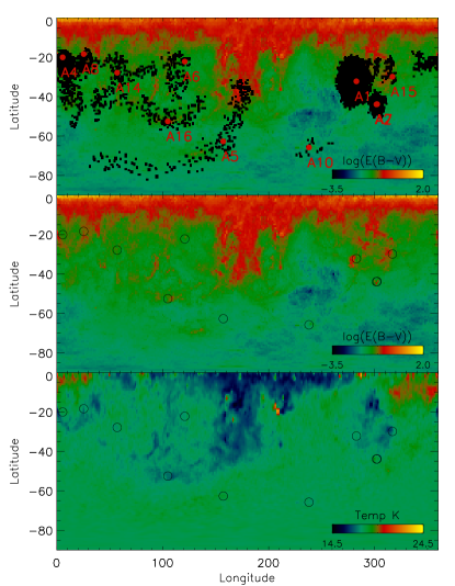
Figure 8.— Comparison of detected structures with features in dust infrared emission maps of Schlegel et al. (1998). The panels show the distribution of dust extinction (top two panels) and dust color temperature (lower panel), as a function of galactic longitude and latitude in the southern hemisphere. The location of the structures are marked as circles on the plots. The top two panels are the same except for the fact that in the top panel, stars associated with the structures in the 2MASS M-giant sample are overplotted. It can be seen that structures A15 and A16 are associated with features both in the extinction and temperature maps.

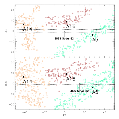
Figure 9.— Plot in R.A. and decl. of groups found in the 2MASS M-giant sample that lie near the SDSS Stripe 82. The filled circles denote the point of peak density while the squares denote the data points belonging to the groups. The bottom panel shows all possible points that can be associated with the density peak of a structure by tracing the particles along the direction of density gradients and have density greater than 0.175 times the peak density of the structure.

4. Results: Structures traced by M-giants in the 2MASS

Table 2Summary of Groups Found in the 2MASS M-giant Sample.

Name	Description	$l$	$b$	$n_{\rm stars}$	Sig $S$	$\rho_{\rm peak}$	Distance
						($\>{\rm kpc}$)
A1	LMC	282.865	-32.231	49234	52.9	2.7 $\times 10^{4}$	$60.1\pm 30$
A2	SMC	301.823	-43.925	4001	33.4	3.0 $\times 10^{4}$	$64.0\pm 32$
A3	Sag leading arm, north	358.130	27.985	3245	27.5	6.5 $\times 10^{1}$	$63.1\pm 32$
A4	Sag core	5.51100	-20.053	1460	24.4	1.8 $\times 10^{3}$	$37.2\pm 19$
A5	Sag trailing arm, south	157.190	-62.682	226	4.82	1.0 $\times 10^{1}$	$37.2\pm 19$
A6	Andromeda	120.819	-22.212	117	4.49	6.5	$122.0\pm 61$
A7	Group in SMC	302.436	-43.837	83	5.13	1.7 $\times 10^{4}$	$48.6\pm 24$
A8	NGC 6822	25.393	-18.378	78	4.74	1.5 $\times 10^{1}$	$92.6\pm 46$
A9	Sag trailing arm, south	187.953	19.882	64	4.54	2.9	$96.6\pm 48$
A10	Fornax dwarf Sph	238.091	-65.798	39	7.58	7.3	$121.3\pm 60$
A11	Near mask	164.086	24.992	79	5.18	3.4	$88.2\pm 44$
A12	Probably Monoceros ring	317.865	21.908	307	5.40	7.5	$21.8\pm 11$
A13	Near mask	143.738	30.936	54	3.93	2.1	$22.6\pm 11$
A14	Has protrusions to high $b$	56.9910	-27.865	203	5.23	8.9	$97.7\pm 48$
A15	Near a strong extinction region	316.906	-29.868	76	4.99	2.7 $\times 10^{1}$	$98.6\pm 49$
A16	In Pisces constellation	104.793	-52.535	126	6.25	9.9	$102.9\pm 51$

Applying our group-finder with $k_{\rm den}=30$ and $S_{\rm Th}=3.75$ to the 2MASS M-giant sample set reveals 16 groups. An Aitoff plot of the groups is shown in LABEL:f7 where each identified group is coded with a unique color and the filled circles mark the position of the densest particle in the group. A summary of the group properties is shown in Table 2. Listed in the table are the name of the groups, the galactic latitude and longitude of the density peak in the groups, the number of stars in the groups, the significance parameter of the groups, the value of peak density and the radial distance of the groups. The first 10 groups listed in the table can be associated with known structures in the Local Group, while the other six are new candidate structures.

Among the known structures that have been identified by the group-finder the densest and most prominent are bound satellite systems such as the Magellanic Clouds (LMC and SMC), and the core of the Sagittarius dwarf galaxy. Unbound debris in the form of the streams from Sagittarius are traced beautifully by means of the structures A3, A5 and A9. Galaxies in the Local Group, like the Andromeda galaxy, NGC 6822 and the Fornax dwarf spheroidal galaxy, which contribute as little as 30-100 stars in the sample, are also re-discovered. These findings both demonstrate the success of the group-finding scheme and lend credibility to the newly discovered structures.

While our group-finding technique has been successful at revealing some of the known structures, others are missing: e.g,. the Virgo overdensity (Jurić et al., 2008), the Virgo stellar stream (Vivas et al., 2001; Duffau et al., 2006), the Canis Major dwarf galaxy (Martin et al., 2004; Martínez-Delgado et al., 2005) and the Hercules Aquila cloud (Belokurov et al., 2007). The absence of these structures can be understood in terms of our sample selection criteria: the Canis Major overdensity is at low latitude ($b=-7^{\circ}.99$) and hence outside the region explored in this paper; the Virgo stellar stream is metal poor $[{\rm Fe/H}]=-1.86$ as suggested by Duffau et al. (2006) and hence is most likely not sampled by the metal rich M-giants; the Virgo overdensity is close to the Sun (6–20 $\>{\rm kpc}$) and largely excluded by our selection criteria of $K_{s}>10.0$ (i.e., distance greater than about 15.0 kpc); the Hercules Aquila cloud is also nearby (10-20 kpc) and , moreover, the part of it in the northern hemisphere is centered at $(l,b)=(30^{\circ},20^{\circ})$, which is outside the region explored by us.

Next we investigate the six newly discovered structures in Table 2. These could have a real physical association with satellite remnants or they could be artificial overdensities created by dust extinction regions, masks, contamination from disk stars or Poisson noise. For example, structures A11, A12, A13 and A14 are all at low latitudes and hence possibly associated with disk. In the cases of structures A11 and A13, both lie right at the edge of one of the rectangular masks (see LABEL:f1 and LABEL:f3) and this further undermines their authenticity. Structure A12 is elongated along the disk, is nearby (distance of about $23\>{\rm kpc}$ ) and its location matches that reported by Rocha-Pinto et al. (2003) for the previously-identified Monoceros ring (see also Yanny et al., 2003; Newberg et al., 2002). Structure A14 also originates at low latitude, but shows a protrusion extending to high latitudes that suggests it could be a real halo structure.

A comparison of the location of the remaining structures (A15 and A16) with the Schlegel et al. (1998) infrared dust emission maps (LABEL:f8) shows that both are associated with high extinction and low temperature features in the maps. The extinction around structure A15 was found to be particularly high while that around A16 is only mildly elevated ($E(B-V)\sim 0.114$ mag). Additionally, A16 is at high latitude and also not close to any masking region and this makes it a promising new structure that could correspond to a satellite accretion event. The close association with a low temperature feature in the dust could either mean that the structure is an artifact of the extinction corrections (improperly deredenned stars getting spuriously included or excluded in our sample) or that the dust feature is associated with the real gas and dust in the structure itself.

Moreover, a structure at a similar location, named the Pisces overdensity, has recently been discovered in a sample of RR Lyrae stars in the SDSS Stripe 82 (Watkins et al., 2009; Sesar et al., 2007). The overdensity has also been spectroscopically confirmed by Kollmeier et al. (2009) using a sample of eight RR Lyraes from SDSS. They speculate it to be a bound satellite system based on the observed velocity dispersion of five of their stars being small ($6\>{\rm km}\,{\rm s}^{-1}$), but at the same time do not rule out the possibility that it is an unbound satellite system due to the large angular width of the overall structure.

To investigate the correspondence of A16 to the Pisces overdensity we plot the groups identified in our 2MASS M-giant sample alongside the SDSS Stripe 82, in the top panel of LABEL:f9. Specifically, the Pisces overdensity has been reported to lie in the interval $-25^{{}^{\circ}}<$R.A.$<0^{{}^{\circ}}$, with the peak concentration being at R.A.$\sim-5^{{}^{\circ}}$ and at a distance of $r=79.9\pm 13.9\>{\rm kpc}$ (as estimated in Watkins et al., 2009). The M-giants in structure A16 are very close to this peak along the boundary of the strip and at a similar distance given the high range of uncertainty ($r=103\>{\rm kpc}$ with a range of $\pm 51$)—the offset in distance could either be due to our arbitrarily adopted value of metallicity in calculating the distances to our stars, or to a dramatic distance gradient across the field.

Given these similarities, it is striking that the upper panel of LABEL:f9 does not show any M-giants from A16 actually in Stripe 82. The most likely explanation for this lack of stars is that the number density of the M-giants associated with the A16 is relatively low within the stripe. Indeed, a comparison of the number of Sagittarius M-giants (group A5) with that of Sagittarius RR Lyraes in Stripe 82 (Watkins et al., 2009) suggests the number of M-giants is probably a factor of 3 lower, implying that the density peak found in RR Lyraes with SDSS should contain only a few M-giants. Hence, the number density of A16 could decrease sufficiently toward the stripe that it is cut off by the default criteria in the group finder itself, which truncates a group whenever it intersects a neighboring group. If we instead relax the default truncation criteria to also include points that converge to the point of peak density in A16 by following the path along local density gradients (i.e., densest nearest neighbor links), we find plausible extensions to the group. The bottom panel of LABEL:f9 plots the positions for this extended group with the minimum density threshold of points being set to 0.175 times the maximum density within a group. Nearby groups extended with the same criteria are also shown alongside. It can be seen that the extended portion of A16 now matches the distribution of Pisces overdensity RR Lyraes in Stripe 82.

We also note that the metallicity of Pisces overdensity has been reported to be $[{\rm Fe/H}]=-1.5$ by Watkins et al. (2009), which means that it would be almost undetectable by M-giants. But at the same time stars in a satellite system do span a range of metallicities, and M-giants could very well be sampling the high metallicity stars in the system.

If A16 and Pisces overdensity are related then A16 not only offers an independent confirmation of the Pisces overdensity, but also provides an extended view of it. In fact our results show that the point of peak density is located at (R.A., decl.)$=(1^{\circ}.81,8^{\circ}.77^{)}$, which is just outside the range of Stripe 82 in SDSS (by about $7^{\circ}$ in decl.). We estimate the uncertainty in the angular position of our peak density to be $\delta\theta=\sin^{-1}(r^{\prime}_{k}/r)=1{\circ}.7$ (where $r$ is the distance of the density peak and $r^{\prime}$ is the radius of the sphere enclosing the fifth nearest neighbor of the densest point)— smaller than the angular distance of the peak from the SDSS Stripe 82. Our results favor an interpretation of unbound satellite system or possibly a bound system within a larger overdensity. Such cloud-like structures are expected to be formed from satellites disrupting along eccentric orbits, while the classical rosette tails (such as those of the Sagittarius dwarf galaxy, see Majewski et al., 2003) arise from objects on more circular orbits (see Johnston et al., 2008, for a more complete discussion of characteristic morphologies).

Finally, note that a smaller sub-concentration of RR Lyrae stars, at a median distance of 92 kpc, has also been noted in the interval $-25^{{}^{\circ}}$ to $-20^{{}^{\circ}}$ of Stripe 82 (structure L in Sesar et al., 2007), which seems to coincide in angular position (see the upper panel of LABEL:f9) and distance with a smaller sub-concentration of stars belonging to structure A14 in the M-giant survey (distances estimated to be 95, 80 and 88 kpc for three M-giants lying in that region). Whether A14 and A16 are truly associated with the structures in RR Lyraes in Stripe 82 (or with each other) can be tested by mapping their velocity and spatial structures.

5. Summary

We have explored the use of a density based hierarchical clustering algorithm to identify structures in the stellar halo. Application of the group finder to a simulated data demonstrated that in three-dimensional data sets with large dispersion in the radial dimension, a coordinate transformation where the radial coordinate is in logarithmic units greatly improves the quality of clustering.

As an application to a real data set we ran the group-finder on the 2MASS M-giant catalog and identified 16 structures in it— 10 of these are known structures and six are new. Among the six new structures, two are probably due to masks employed on the data, one is associated with a strong extinction region, and one is probably a part of the Monoceros ring. Another one originates at low latitude, suggesting contamination by disk stars, but also shows significant protrusions extending to high latitudes implying that it is a real feature in the stellar halo.

One structure is free from these defects, has an overdensity similar to that of known structures like the streams of the Sagittarius dwarf galaxy and is also slightly above the Poisson noise. While these properties suggest that it is a genuine structure, possibly a satellite remnant, the structure was also found to match a low temperature feature in the dust map. The correspondence with a feature in dust map could either mean that the structure is an artifact of the extinction corrections or that the dust feature is associated with the real gas and dust in the structure itself.

The position and distance of the detected structure closely match those of the Pisces overdensity, which has been recently discovered using RR Lyraes in the SDSS Stripe 82. If A16 is indeed related to Pisces overdensity then our analysis using 2MASS M-giants provides an independent confirmation of the overdensity and offers an extended view of it. In addition, our analysis suggests that the peak point of density is located just outside the range of the SDSS stripe, which favors the interpretation that the system is an unbound satellite system, probably corresponding to a debris from a satellite disrupting along a fairly radial orbit. Deeper photometric surveys of this region along with spectroscopic measurements of the giant stars associated with the overdensity should help confirm or rule out this scenario.

Overall we conclude that group finding is a promising technique to unravel the history of our stellar halo and as a window on accretion more generally. Clouds of debris like the Pisces overdensity are naturally found in model stellar halos built within a standard cosmological context, and are even predicted to be the dominant structures in the outer halo (Bullock & Johnston, 2005; Johnston et al., 2008). Indeed, if none were found we would conclude either that we live in a Galaxy that has suffered an unusual paucity of accretion events on radial orbits, or that our expectations of orbital distributions of accreting objects (gleaned from cosmological simulations of structure formation) are flawed.

Future prospects for group-finding are even brighter: our analysis here has only used the three-dimensional spatial distribution of stars while many surveys also have velocity (proper motions and radial velocities of stars) and chemical abundance information. These additional dimensions should help recover more structures. Moreover, we have here used M-giants as tracers of the stellar halo. Since M-giants are metal rich stars this means that our sample is biased toward high-metallicity systems that originate from high mass progenitors and misses out on the much more numerous low mass systems that have low metallicity. Hence surveys utilizing a different tracer population, e.g., main sequence stars or RR Lyraes should unravel more structures in the stellar halo.

References

- Bell et al. (2008) Bell, E. F., et al. 2008, ApJ, 680, 295
- Belokurov et al. (2007) Belokurov, V., et al. 2007, ApJ, 657, L89
- Bertelli et al. (1994) Bertelli, G., Bressan, A., Chiosi, C., Fagotto, F., & Nasi, E. 1994, A&AS, 106, 275
- Bonatto et al. (2004) Bonatto, C., Bica, E., & Girardi, L. 2004, A&A, 415, 571
- Bullock & Johnston (2005) Bullock, J. S., & Johnston, K. V. 2005, ApJ, 635, 931
- Bullock et al. (2001) Bullock, J. S., Kravtsov, A. V., & Weinberg, D. H. 2001, ApJ, 548, 33
- Duffau et al. (2006) Duffau, S., Zinn, R., Vivas, A. K., Carraro, G., Méndez, R. A., Winnick, R., & Gallart, C. 2006, ApJ, 636, L97
- Eke et al. (2004) Eke, V. R., et al. 2004, MNRAS, 348, 866
- Helmi & White (1999) Helmi, A., & White, S. D. M. 1999, MNRAS, 307, 495
- Ibata et al. (1994) Ibata, R. A., Gilmore, G., & Irwin, M. J. 1994, Nature, 370, 194
- Ibata et al. (1995) —. 1995, MNRAS, 277, 781
- Ivezic et al. (2009) Ivezic, Z., et al. 2009, in Bulletin of the American Astronomical Society, Vol. 41, Bulletin of the American Astronomical Society, 366–+
- Jenkins et al. (2001) Jenkins, A., Frenk, C. S., White, S. D. M., Colberg, J. M., Cole, S., Evrard, A. E., Couchman, H. M. P., & Yoshida, N. 2001, MNRAS, 321, 372
- Johnston (1998) Johnston, K. V. 1998, ApJ, 495, 297
- Johnston et al. (2008) Johnston, K. V., Bullock, J. S., Sharma, S., Font, A., Robertson, B. E., & Leitner, S. N. 2008, ApJ, 689, 936
- Jurić et al. (2008) Jurić, M., et al. 2008, ApJ, 673, 864
- Keller et al. (2007) Keller, S. C., et al. 2007, Publications of the Astronomical Society of Australia, 24, 1
- Kollmeier et al. (2009) Kollmeier, J. A., et al. 2009, ApJ, 705, L158
- Lacey & Cole (1993) Lacey, C., & Cole, S. 1993, MNRAS, 262, 627
- Majewski et al. (2004) Majewski, S. R., Ostheimer, J. C., Rocha-Pinto, H. J., Patterson, R. J., Guhathakurta, P., & Reitzel, D. 2004, ApJ, 615, 738
- Majewski et al. (2003) Majewski, S. R., Skrutskie, M. F., Weinberg, M. D., & Ostheimer, J. C. 2003, ApJ, 599, 1082
- Marigo et al. (2008) Marigo, P., Girardi, L., Bressan, A., Groenewegen, M. A. T., Silva, L., & Granato, G. L. 2008, A&A, 482, 883
- Martin et al. (2004) Martin, N. F., Ibata, R. A., Bellazzini, M., Irwin, M. J., Lewis, G. F., & Dehnen, W. 2004, MNRAS, 348, 12
- Martin et al. (2005) Martin, N. F., Ibata, R. A., Conn, B. C., Lewis, G. F., Bellazzini, M., & Irwin, M. J. 2005, MNRAS, 362, 906
- Martin et al. (2007) Martin, N. F., Ibata, R. A., & Irwin, M. 2007, ApJ, 668, L123
- Martínez-Delgado et al. (2005) Martínez-Delgado, D., Butler, D. J., Rix, H., Franco, V. I., Peñarrubia, J., Alfaro, E. J., & Dinescu, D. I. 2005, ApJ, 633, 205
- Newberg et al. (2002) Newberg, H. J., et al. 2002, ApJ, 569, 245
- Peñarrubia et al. (2005) Peñarrubia, J., et al. 2005, ApJ, 626, 128
- Perryman (2002) Perryman, M. A. C. 2002, Ap&SS, 280, 1
- Pfitzner et al. (1997) Pfitzner, D. W., Salmon, J. K., & Sterling, T. 1997, Data Min. Knowl. Discov., 1, 419
- Reed et al. (2007) Reed, D. S., Bower, R., Frenk, C. S., Jenkins, A., & Theuns, T. 2007, MNRAS, 374, 2
- Rocha-Pinto et al. (2003) Rocha-Pinto, H. J., Majewski, S. R., Skrutskie, M. F., & Crane, J. D. 2003, ApJ, 594, L115
- Rocha-Pinto et al. (2004) Rocha-Pinto, H. J., Majewski, S. R., Skrutskie, M. F., Crane, J. D., & Patterson, R. J. 2004, ApJ, 615, 732
- Schlegel et al. (1998) Schlegel, D. J., Finkbeiner, D. P., & Davis, M. 1998, ApJ, 500, 525
- Sesar et al. (2007) Sesar, B., et al. 2007, AJ, 134, 2236
- Sharma & Johnston (2009) Sharma, S., & Johnston, K. V. 2009, ApJ, 703, 1061
- Springel et al. (2001) Springel, V., White, S. D. M., Tormen, G., & Kauffmann, G. 2001, MNRAS, 328, 726
- Vivas et al. (2001) Vivas, A. K., et al. 2001, ApJ, 554, L33
- Watkins et al. (2009) Watkins, L. L., et al. 2009, MNRAS, 398, 1757
- Yanny et al. (2003) Yanny, B., et al. 2003, ApJ, 588, 824