Defect Modes and Homogenization of Periodic Schrödinger Operators

Abstract

We consider the discrete eigenvalues of the operator $H_{\varepsilon}=-\Delta+V(\mathbf{x})+\varepsilon^{2}Q(\varepsilon\mathbf{x})$, where $V(\mathbf{x})$ is periodic and $Q(\mathbf{y})$ is localized on $\mathbb{R}^{d},\ \ d\geq 1$. For $\varepsilon>0$ and sufficiently small, discrete eigenvalues may bifurcate (emerge) from spectral band edges of the periodic Schrödinger operator, $H_{0}=-\Delta_{\mathbf{x}}+V(\mathbf{x})$, into spectral gaps. The nature of the bifurcation depends on the homogenized Schrödinger operator $L_{A,Q}=-\nabla_{\mathbf{y}}\cdot A\nabla_{\mathbf{y}}+\ Q(\mathbf{y})$. Here, $A$ denotes the inverse effective mass matrix, associated with the spectral band edge, which is the site of the bifurcation.

1 Introduction and Outline

Self-adjoint elliptic partial differential operators with periodic coefficients e.g. the Schrödinger operator with a periodic potential, the time-harmonic Helmholtz equation with variable refractive index, and the time-harmonic Maxwell equations with variable dielectric and permeability tensors, play a central role in wave propagation problems in classical and quantum physics. The spectrum of such operators, characterized by Floquet-Bloch theory [29, 20, 12], consists of the union of closed intervals (spectral bands). The eigenstates are extended (not localized) and form a complete set with respect to which any function in $L^{2}(\mathbb{R}^{d})$ may be represented.

In many problems in fundamental and applied physics, periodic media are perturbed by spatially localized defects. These may appear as random imperfections in a media, e.g. a defect in a crystal, or in engineering applications, they may be introduced deliberately in order to influence wave propagation [4, 17]. Since the essential spectrum is unchanged by a sufficiently localized and smooth perturbation (Weyl’s theorem, [29]), typical localized perturbations will only introduce eigenvalues in spectral gaps of the spectrum with associated localized defect modes.

This paper is concerned with a class of localized (defect) perturbations to a periodic Schrödinger operator of the form:

$$H_{\varepsilon}\ =\ -\Delta_{\mathbf{x}}+V(\mathbf{x})+\varepsilon^{2}Q(\varepsilon\mathbf{x}),$$

where $V(\mathbf{x})$ is periodic on $\mathbb{R}^{d}$, $Q(\mathbf{y})$ decays as $|\mathbf{y}|$ tends to infinity and $\varepsilon$ is a small parameter.

Our main result, Theorem 2, concerns the perturbed eigenvalue problem

$$\begin{split}H_{\varepsilon}u_{\varepsilon}=\mu_{\varepsilon}u_{\varepsilon},\quad u_{\varepsilon}\in H^{1}(\mathbb{R}^{d}),\end{split}$$ (1)

for $\varepsilon$ positive and sufficiently small. See section 3 for hypotheses on the periodic potential, $V$, and the localized perturbation, $Q$.

For $\varepsilon$ sufficiently small, we prove the bifurcation of discrete eigenvalues into the spectral gaps, associated with the unperturbed operator, $H_{0}=-\Delta+V(\mathbf{x})$. For any given spectral band edge, we give detailed expansions with error estimates for the perturbed eigenvalues and corresponding localized eigenfunctions in terms of the eigenstates of a homogenized Schrödinger operator

$$L_{A,Q}\ =\ -\sum_{j,l=1}^{d}\ \frac{\partial}{\partial y_{j}}\ A_{jl}\ \frac{\partial}{\partial y_{l}}\ +\ Q(\mathbf{y}).$$ (2)

Here, $A_{jl}$ denotes the inverse effective mass matrix, associated with the particular band edge from which the bifurcation occurs; see Theorem 2. $A_{jl}$, derivable by formal multiple scale expansion (see section 4), is expressible in terms of the band edge (Floquet-Bloch) eigenstate. It is proportional to the Hessian matrix $D^{2}E_{b_{*}}(\mathbf{k}_{*})$ of the band dispersion function, associated with $-\Delta+V(\mathbf{x})$, evaluated at the band edge $E_{*}=E_{b_{*}}(\mathbf{k}_{*})$.

Referring to the schematics of figures 1 and 2, we discuss our results.

• Suppose the inverse effective mass matrix, $A$, is positive definite and assume $L_{A,Q}$ has an eigenvalue, $e_{A,Q}<0$. This occurs if $Q(\mathbf{y})$ is a “down-defect” (sufficiently “deep” in dimensions $d\geq 3$) as in figure 1.a. In this case, Theorem 2 asserts the existence of an eigenvalue at $E_{*}+\varepsilon^{2}e_{A,Q}+{\cal O}(\varepsilon^{3})<E_{*}$.

• Now suppose the inverse effective mass matrix, $A$, is negative definite and $L_{A,Q}$ has an eigenvalue, $e_{A,Q}>0$. This occurs if $Q(\mathbf{y})$ is a “up-defect” (sufficiently “high” in dimensions $d\geq 3$) as in figure 1.b. In this case, Theorem 2 asserts the existence of an eigenvalue at $E_{*}+\varepsilon^{2}e_{A,Q}+{\cal O}(\varepsilon^{3})>E_{*}$

• Fig. 2 shows a more general band edge bifurcation when $L_{A,Q}$ has three eigenvalues $e_{A,Q}^{(1)}<e_{A,Q}^{(2)}<e_{A,Q}^{(3)}$, the largest of which is degenerate with multiplicity three. Theorem 2 asserts the existence of five ordered eigenvalues at $E_{*}+\varepsilon^{2}e_{A,Q}^{(j)}+{\cal O}(\varepsilon^{3}),\ j=1,2$ and $E_{*}+\varepsilon^{2}e_{A,Q}^{(3)}+\varepsilon^{3}\mu_{3}^{(k)}+{\cal O}(\varepsilon^{4}),\ k=1,2,3$.

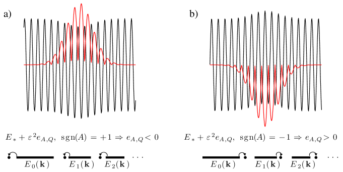
Fig. 1: a) Periodic structure with “down defect” and corresponding localized eigenstate for the case of positive definite effective mass tensor. b) Periodic structure with “up defect” and corresponding localized eigenstate for the case of negative definite effective mass tensor. Below are shown eigenvalue bifurcations from band edges of the form $E_{b_{*}}(\mathbf{k}_{*})=E_{*}$.

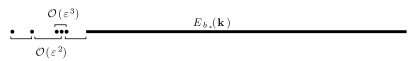
Fig. 2: Schematic of band edge bifurcations in the case where the inverse effective mass matrix, $A$, is positive definite. The homogenized operator, $L_{A,Q}$, is assumed to have two simple eigenvalues and one degenerate eigenvalue with multiplicity three.

1.1 Outline of the paper and overview of the proof

Section 2 summarizes the required spectral theory for Schrödinger operators with periodic potentials and introduces variants of the classical Sobolev space, $H^{s}(\mathbb{R}^{d})$, which provide a natural functional analytic setting. Section 3 contains the hypotheses on $V$ and $Q$ and the statement of our main theorem, Theorem 2. In section 4 we present a formal multiple scale / homogenization expansion in which we systematically construct bifurcating eigenstates and eigenvalues to any prescribed order. In section 5 we prove Theorem 2. In particular, we study the equations governing the correction, $\Psi^{\varepsilon}$ to the $N-$ term multiple scale expansion.

To obtain error bounds of suitably high order in $\varepsilon$, we use a Lyapunov-Schmidt approach. Specifically, we decompose the error into Floquet-Bloch modes associated with energies lying near the spectral band edge, $E_{*}$, and those lying “far” from $E_{*}$: $\Psi^{\varepsilon}=\Psi^{\varepsilon}_{\rm near}+\Psi^{\varepsilon}_{\rm far}$. $\Psi^{\varepsilon}_{\rm near}$ has the character of a wave-packet, spectrally supported on a small interval with endpoint $E_{*}$. The next step is to solve for $\Psi^{\varepsilon}_{\rm far}$ as a functional of the “parameter” $\Psi^{\varepsilon}_{\rm near}$, with appropriate bounds. Substitution of $\Psi^{\varepsilon}_{\rm far}[\Psi^{\varepsilon}_{\rm near}]$ into the near equation implies a closed equation for $\Psi^{\varepsilon}_{\rm near}$. With strong motivation from the structure of terms in the multiple scale expansion, we appropriately rescale, solve via the implicit function theorem, and estimate $\Psi^{\varepsilon}_{\rm near}$. The approach we take has been applied in the context of the nonlinear Schrödinger / Pitaevskii equation in [31, 27, 10, 9, 16].

Previous work for linear Schrödinger operators: Bifurcation of eigenvalues from the edge of the continuous spectrum for Schrödinger operators with small decaying potentials, corresponding to weak defects in dimensions one and two for the case of a homogeneous medium or vacuum ($V\equiv 0$), was studied in [30]. Conditions ensuring the existence of eigenvalues in the gaps of periodic potentials were obtained in [1] and [13, 14], using the Birman-Schwinger (integral equation) formulation of the eigenvalue problem. Homogenization theory was applied to obtain eigenvalues in the spectral gaps of a class of periodic divergence form elliptic operators, governing localized states in high contrast media in [18, 8]. An elementary variational argument in spatial dimensions one and two, yielding general conditions for the existence of discrete modes in spectral gaps of periodic potentials, was recently presented in [26]. More general, variational methods can be applied to obtain defect modes which are obtained as infinite dimensional saddle points of strongly indefinite functionals; see, for example, [11].

Our results concern a particular class of weak defects, slowly varying and of small amplitude: $\varepsilon^{2}Q(\varepsilon\mathbf{x})$, which give rise to defect modes in any spatial dimension. We note that the one- and two-term truncated multi-scale homogenization expansion of defect modes, which we construct, are natural trial functions for a variational proof of existence of ground states; see the discussion in Appendix B. Note also that the scaling of the perturbing potential, $\varepsilon^{2}Q(\varepsilon\mathbf{x})$, also arises naturally in solitary standing wave (“soliton defect mode”) bifurcations from band edges of periodic potentials in the nonlinear Schrödinger / Gross-Pitaevskii equation [16].

Homogenization theory has been used to study periodic elliptic divergence form operators near spectral band edges in [6, 7, 2]. Homogenization results for the time-dependent Schrödinger equation with a scaling, equivalent to the one considered here, were obtained by two-scale convergence methods in [3]; see also [28, 5, 2]. In [3] the contrast between the scaling we use and the semi-classical scaling is discussed. These results establish the validity of the homogenized time-dependent Schrödinger equation on certain finite time scales. The results of the present paper focus on a subclass of solutions, bound states, which are controlled on infinite time scales.

Finally, we mention work on effective classical electron motion in solid state physics, derived from the Schrödinger equation for an electron in a spatially periodic Hamiltonian, perturbed by spatially slowly varying electrostatic and magnetic potentials [22, 24, 25], in a semi-classical limit.

Acknowledgments: This research was initiated while MAH was an NSF Postdoctoral Fellow under DMS-08-03074 in the Department of Applied Physics and Applied Mathematics at Columbia University. MIW was supported in part by NSF grant DMS-07-07850 and DMS-10-08855. MIW would also like to acknowledge the hospitality of the Courant Institute of Mathematical Sciences, where he was on sabbatical during the preparation of this article.

1.2 Notation and conventions

We note that we may, without loss of generality, restrict to the case where the fundamental period cell is $\Omega=[0,1]^{d}$. Indeed, let ${\cal B}$ denote the fundamental period cell, spanned by the linearly independent vectors $\{{\bf r}_{1},\dots,{\bf r}_{d}\}$ and define the constant matrix ${\cal R}^{-1}$ to be the matrix whose $j^{\rm th}$ column is ${\bf r}_{j}$. Then, under the change of coordinates ${\bf x}\mapsto{\bf z}={\cal R}{\bf x}$,

$$-\nabla_{\bf x}\cdot\nabla_{\bf x}\ +\ V({\bf x})\ {\rm acting\ on}\ L_{\textrm{per}}^{2}({\cal B})\ \ {\rm transforms\ to}$$

$$-\nabla_{\bf z}\cdot\alpha\ \nabla_{\bf z}+\tilde{V}({\bf z})\equiv\ -\ \sum_{i,j=1}^{d}\alpha_{ij}\ \frac{\partial^{2}}{\partial z_{i}\partial z_{j}}\ +\ \tilde{V}({\bf z})$$

$${\rm acting\ on}\ L^{2}_{\textrm{per}}\left([0,1]^{d}\right)\ {\rm where}$$

$$\alpha={\cal R}{\cal R}^{T},\ \ \tilde{V}({\bf z})=V\left({\cal R}^{-1}{\bf z}\right),\ \ {\bf x}={\cal R}^{-1}{\bf z}\ .$$

1. Integrals with unspecified region of integration are assumed to be taken over $\mathbb{R}^{d}$, i.e. $\int f\ =\int_{\mathbb{R}^{d}}f(\mathbf{x})d\mathbf{x}$.

2. For $f,g\in L^{2}$, the Fourier transform and its inverse are given by:

   $$\mathcal{F}\{f\}(\mathbf{k}) \equiv\widehat{f}(\mathbf{k})=\int e^{-2\pi i\mathbf{k}\cdot\mathbf{x}}f(\mathbf{x})\,d\mathbf{x},$$ (3)

   $$\mathcal{F}^{-1}\{g\}(\mathbf{x}) \equiv\ \widecheck{g}(\mathbf{k})=\int e^{2\pi i\mathbf{x}\cdot\mathbf{k}}g(\mathbf{k})\,d\mathbf{k}.$$

   Thus, $\mathcal{F}\ \mathcal{F}^{-1}=Id$.

3. $\Omega=[0,1]^{d}$ is the fundamental period cell, $\Omega^{*}=[-1/2,1/2]^{d}$ is the dual fundamental cell or Brillouin zone

4. $1_{A}(\mathbf{x})$ is the indicator function of the set $A$; $\chi(|\mathbf{k}|\leq a)\equiv 1_{\{\mathbf{k}\in\Omega^{*}\,:\,|\mathbf{k}|\leq a\}}$

5. The repeated index summation convention is used throughout

6. Fourier spectral cutoff:

   $$\chi(|\nabla|<a)G(\mathbf{x}) \equiv\ \left({\cal F}^{-1}\chi(|\mathbf{k}|<a){\cal F}\right)G\ =\ \int e^{2\pi i\mathbf{x}\cdot\mathbf{k}}\chi(|\mathbf{k}|<a)\widehat{G}(\mathbf{k})d\mathbf{k}$$

7. ${\cal T}$ and ${\cal T}^{-1}$ denote the Gelfand-Bloch transform and its inverse; see section 2.

8. Bloch spectral cutoff:

   $$\chi(|\nabla|<a)G(\mathbf{x}) \equiv\mathcal{T}^{-1}\left\{\sum_{b\geq 0}\chi(|\cdot|<a\delta_{bb_{*}})\mathcal{T}_{b}\left\{G\right\}(\cdot)\,p_{b}(\mathbf{x};\cdot)\right\}(\mathbf{x}),$$

   where $b_{*}$ is the index of the spectral band under consideration,

9. $H^{s}=H^{s}(\mathbb{R}^{d})$ is the Sobolev space of order $s$

   $$\|f\|_{H^{s}}^{2}\equiv\sum_{|\alpha|\leq s}\|\partial^{\alpha}f\|^{2}_{L^{2}}\sim\|\widehat{f}\|_{L^{2,s}}^{2}=\int_{\mathbb{R}^{d}}(1+|\mathbf{k}|^{s\over 2})^{2}|\hat{f}(\mathbf{k})|^{2}\,d\mathbf{k}$$ (5)

2 Spectral Theory for Periodic Potentials

In this section we summarize basic results on the spectral theory of Schrödinger operators with periodic potentials; see, for example, [29, 20, 12].

Gelfand-Bloch transform:  Given $f\in L^{2}(\mathbb{R}^{d})$, we introduce the transform $\mathcal{T}$ and its inverse as follows

$$\mathcal{T}\{f(\cdot)\}(\mathbf{x};\mathbf{k})= \tilde{f}(\mathbf{x};\mathbf{k})=\sum_{\mathbf{z}\in\mathbb{Z}^{d}}e^{2\pi i\mathbf{z}\cdot\mathbf{x}}\widehat{f}(\mathbf{k}+\mathbf{z}),$$ (6)

$$\mathcal{T}^{-1}\{\tilde{f}(\mathbf{x};\cdot)\}(\mathbf{x}) =\int_{\Omega^{*}}e^{2\pi i\mathbf{x}\cdot\mathbf{k}}\tilde{f}(\mathbf{x};\mathbf{k})d\mathbf{k}.$$ (7)

One can check that $\mathcal{T}^{-1}\mathcal{T}=Id$.

Two important properties of the transformation $\mathcal{T}$ are $\mathcal{T}\partial_{x_{j}}f=\left(\partial_{x_{j}}+2\pi ik_{j}\right)\mathcal{T}f$ and $\left(\mathcal{T}e^{2\pi i\mathbf{k}\cdot}f\right)(\mathbf{x},\mathbf{k})=e^{2\pi i\mathbf{k}\cdot\mathbf{x}}\mathcal{T}f(\mathbf{x},\mathbf{k})$. It follows that

$$\left(\mathcal{T}\Phi(\nabla)e^{2\pi i\mathbf{k}\cdot}f\right)(\mathbf{x},\mathbf{k}) =e^{2\pi i\mathbf{k}\cdot x}\Phi(\nabla+2\pi i\mathbf{k})\left(\mathcal{T}f\right)(\mathbf{x},\mathbf{k})$$ (8)

$$\mathcal{T}\left(v(\cdot)f\right)(\mathbf{x},\mathbf{k}) =v(\mathbf{x})\left(\mathcal{T}f\right)(\mathbf{x},\mathbf{k}),\ \ {\rm if\ }v\ {\rm is\ periodic.}$$ (9)

Floquet-Bloch states: We seek solutions of the eigenvalue equation

$$\left(-\Delta+V(\mathbf{x})\right)u(\mathbf{x})=Eu(\mathbf{x})$$ (10)

in the form $u(\mathbf{x};\mathbf{k})=e^{2\pi i\mathbf{k}\cdot\mathbf{x}}p(\mathbf{x};\mathbf{k}),\ \mathbf{k}\in\Omega^{*}$ where $p(\mathbf{x};\mathbf{k})$ is periodic in $\mathbf{x}$ with fundamental period cell $\Omega$. $p(\mathbf{x};\mathbf{k})$ then satisfies the periodic elliptic boundary value problem:

$$\left(-\left(\nabla+2\pi i\mathbf{k}\right)^{2}+V(\mathbf{x})\right)p(\mathbf{x};\mathbf{k})=E(\mathbf{k})p(\mathbf{x};\mathbf{k}),\quad\mathbf{x}\in\mathbb{T}^{d}.$$ (11)

For each $\mathbf{k}\in\Omega^{*}$, the eigenvalue problem (11) has a discrete set of eigenpairs
$\{\ p_{b}(\mathbf{x};\mathbf{k}),\ E_{b}(\mathbf{k})\ \}_{b\geq 0}$ which form a complete orthonormal set in $L^{2}_{\rm per}(\Omega)$. The spectrum of $-\Delta+V(\mathbf{x})$ in $L^{2}(\mathbb{R}^{d})$ is the union of closed intervals

$$\textrm{spec}(-\Delta+V)=\bigcup_{b\geq 0,~{}\mathbf{k}\in\Omega^{*}}E_{b}(\mathbf{k}).$$ (12)

We will study the bifurcation of eigenvalues from the band edge

$$E_{*}\equiv E_{b_{*}}(\mathbf{k}_{*}),\quad k_{*,j}\in\{0,1/2\},\quad j=1,\ldots,d,$$ (13)

with the associated, real-valued band edge eigenfunction

$$w(\mathbf{x})\equiv e^{2\pi i\mathbf{k}_{*}\cdot\mathbf{x}}p_{b_{*}}(\mathbf{x};\mathbf{k}_{*})\in L^{2}(\Omega).$$ (14)

For example, the lowest band edge is $E_{0}(0)$ and the associated eigenfunction is periodic $p_{0}(\mathbf{x}+\mathbf{e}_{j};0)=p_{0}(\mathbf{x};0)$, $j=1,\ldots,d$ for the standard Cartesian basis vectors $\{\mathbf{e}_{j}\}_{j=1}^{d}$.

Remark 2.1.

Since

$$w(\mathbf{x}+\mathbf{e}_{j})=e^{2\pi ik_{*,j}}w(\mathbf{x})=s_{j}w(\mathbf{x}),$$ (15)

where $s_{j}=+1$ if $k_{*,j}=0$ and $s_{j}=-1$ otherwise, the natural function space to work in is $L^{2}_{\textrm{symm}}(\Omega)$, i.e. $f\in L^{2}_{\textrm{symm}}(\Omega)$ if $f\in L^{2}(\Omega)$ and $f(\mathbf{x}+\mathbf{e}_{j})=s_{j}f(\mathbf{x})$. Without loss of generality, and for ease of presentation, we focus on the case where $s_{j}=+1$, $j=1,\ldots,d$ so that $L^{2}_{\textrm{symm}}(\Omega)=L^{2}_{\textrm{per}}(\Omega)$, the space of square integrable, periodic functions. This implies that $\mathbf{k}_{*}=0$. The more general case in eq. (13) can be handled by taking $\mathbf{k}\to(\mathbf{k}-\mathbf{k}_{*})$ and interpreting values of $\mathbf{k}$ reflected about the boundary of $\Omega^{*}$. The simplicity of $E_{*}$ and the relation $\nabla E_{b_{*}}(\mathbf{k}_{*})=0$ (see Hypothesis H2 in Sec. 3) implies that $E(\mathbf{k}^{\prime}+\mathbf{k}_{*})$ can be extended as an even function of $k^{\prime}_{j}=k_{j}-k_{j,*}$ for $j=1,\ldots,d$ [29].

We will make repeated use of the following self-adjoint operator

$$L_{*}\equiv-\Delta+V(\mathbf{x})-E_{*}:H_{\textrm{per}}^{2}(\Omega)\to L^{2}(\Omega).$$ (16)

Projections $\mathcal{T}_{b}$ and Completeness of Floquet Bloch states: Define

$$\mathcal{T}_{b}\{f\}(\mathbf{k})\equiv\langle p_{b}(\cdot;\mathbf{k}),\tilde{f}(\cdot;\mathbf{k})\rangle_{L^{2}(\Omega)}\equiv\int_{\Omega}\overline{p_{b}(\mathbf{x};\mathbf{k})}\ \tilde{f}(\mathbf{x};\mathbf{k})\,d\mathbf{x}.$$ (17)

By completeness of the $\{p_{b}(\mathbf{x};\mathbf{k})\}_{b\geq 0}$

$$\tilde{f}(\mathbf{x};\mathbf{k})=\sum_{b\geq 0}\mathcal{T}_{b}\{f\}(\mathbf{k})\ p_{b}(\mathbf{x};\mathbf{k})$$

Furthermore, applying ${\cal T}^{-1}$ we have

$$f(\mathbf{x}) =\sum_{b\geq 0}\int_{\Omega^{*}}\ \mathcal{T}_{b}\{f\}(\mathbf{k})\ u_{b}(\mathbf{x};\mathbf{k})\ d\mathbf{k}$$ (18)

$$=\sum_{b\geq 0}\ \int_{\Omega^{*}}\ \langle u_{b}(\cdot;\mathbf{k}),f\rangle_{L^{2}(\mathbb{R}^{d})}\ u_{b}(\mathbf{x};\mathbf{k})\ d\mathbf{k},$$ (19)

where $u_{b}(\mathbf{x};\mathbf{k})=e^{2\pi i\mathbf{k}\cdot\mathbf{x}}p_{b}(\mathbf{x};\mathbf{k})$. The second equality follows from an application of the Poisson summation formula.

Sobolev spaces and the Gelfand-Bloch transform:
Recall the Sobolev space, $H^{s}$, the space of functions with square-integrable derivatives of order $\leq s$. Since $E_{0}(0)=\inf\ {\rm spec}(-\Delta+V)$, then $L_{0}=-\Delta+V(\mathbf{x})-E_{0}(0)$ is a non-negative operator and $H^{s}(\mathbb{R}^{d})$ has the equivalent norm defined by

$$\|\phi\|_{H^{s}}\ \sim\ \|(I+L_{0})^{s\over 2}\phi\|_{L^{2}}\$$

Introduce the space (see, e.g. [27, 9])

$${\cal X}^{s}=L^{2}(\Omega^{*},l^{2,s}),$$ (20)

with norm

$$\|\tilde{\phi}\|^{2}_{{\cal X}^{s}}\equiv\int_{\Omega^{*}}\sum_{b=0}^{\infty}\left(1+|b|^{2\over d}\right)^{s}|\mathcal{T}_{b}\{\phi\}(\mathbf{k})|^{2}\,d\mathbf{k}.$$ (21)

Now note that

$$\|\phi\|_{H^{s}}^{2} \sim\|(I+L_{0})^{s\over 2}\phi\|_{L^{2}}^{2}\$$

$$=\ \left\|\ \int_{\Omega^{*}}\ e^{2\pi i\mathbf{k}\cdot}\sum_{b\geq 0}\mathcal{T}_{b}\{\phi\}(\mathbf{k})\left(1+E_{b}(\mathbf{k})-E_{0}(0)\right)^{\frac{s}{2}}\ p_{b}(\cdot,\mathbf{k})\ d\mathbf{k}\right\|_{L^{2}}^{2}$$

$$=\sum_{b\geq 0}\ \int_{\Omega^{*}}\ |\mathcal{T}_{b}\{\phi\}(\mathbf{k})|^{2}\ |1+E_{b}(\mathbf{k})-E_{0}(0)|^{s}\ d\mathbf{k}$$

$$\sim\ \sum_{b\geq 0}\ \left(1+|b|^{2\over d}\right)^{s}\ \int_{\Omega^{*}}\ |\mathcal{T}_{b}\{\phi\}(\mathbf{k})|^{2}\ d\mathbf{k}$$

$$\equiv\|\tilde{\phi}\|^{2}_{{\cal X}^{s}}.$$ (22)

The second to last line follows from the Weyl asymptotics $E_{b}(\mathbf{k})\sim b^{2\over d}$ [15]. Thus we have

Proposition 1.

$H^{s}(\mathbb{R}^{d})$ is isomorphic to ${\cal X}^{s}$ for $s\geq 0$. Moreover, there exist positive constants $C_{1}$, $C_{2}$ such that for all $\phi\in H^{s}(\mathbb{R}^{d})$

$$C_{1}\|\phi\|_{H^{s}(\mathbb{R}^{d})}\leq\|\tilde{\phi}\|_{{\cal X}^{s}}\leq C_{2}\|\phi\|_{H^{s}(\mathbb{R}^{d})}\ .$$ (23)

3 Main Results

In this section we give a precise formulation of our main theorem, Theorem 2. The following are our assumptions.

• Regularity. $V\in L^{\infty}_{\textrm{per}}(\Omega)$, $Q\in H^{\sigma}(\mathbb{R}^{d})$ for $\sigma>d$, $E_{b_{*}}\in C^{3}(\Omega^{*})$, and $p_{b_{*}}\in L^{2}_{\textrm{per}}(\Omega;C^{3}(\Omega^{*}))$.

• Band edge. $E_{*}\equiv E_{b_{*}}(\mathbf{k}_{*})$, where $\mathbf{k}_{*}$ is an endpoint of the $b_{*}^{th}$ band such that

  (a) $E_{*}$ is a simple eigenvalue with corresponding eigenfunction

  $$w(\mathbf{x})\equiv e^{2\pi i\mathbf{k}_{*}\cdot\mathbf{x}}p_{b_{*}}(\mathbf{x};\mathbf{k}_{*})\in H^{2}_{\textrm{per}}(\Omega)$$

  and normalization $\|w\|_{L^{2}(\Omega)}=1$.

  (b) $\nabla E_{b_{*}}(\mathbf{k}_{*})=0$.

  (c) The Hessian matrix,

  $$A\equiv\frac{1}{8\pi^{2}}D^{2}E_{b_{*}}(\mathbf{k}_{*}),$$ (24)

  is sign definite.

• Existence of eigenvalue to homogenized equation.
  Introduce the homogenized operator

  $$L_{A,Q}\ \equiv-\nabla_{\mathbf{y}}\cdot A\ \nabla_{\mathbf{y}}+Q(\mathbf{y})\ =\ -\sum_{j,l}\frac{\partial}{\partial y_{j}}A_{jl}\frac{\partial}{\partial y_{l}}+Q(\mathbf{y})$$ (25)

  Set $\textrm{sgn}(A)=+1$ if $A$ is positive definite and $\textrm{sgn}(A)=-1$ if $A$ is negative definite. Assume $L_{A,Q}$ has a simple eigenvalue $e_{A,Q}$ with $\textrm{sgn}(A)e_{A,Q}<0$ and corresponding eigenfunction $F_{A,Q}(\mathbf{y})\in H^{2}(\mathbb{R}^{d})$; i.e.

  $$L_{A,Q}F_{A,Q}=e_{A,Q}F_{A,Q},\quad\int_{\mathbb{R}^{d}}F_{A,Q}^{2}(\mathbf{y})d\mathbf{y}=1,\quad\textrm{sgn}(A)\,e_{A,Q}<0;$$ (26)

  see figure 3(a).

  

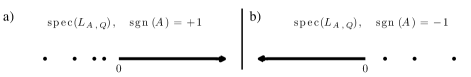
  Fig. 3: Discrete and continuous spectrum of $L_{A,Q}$. a) Positive definite effective mass tensor. b) Negative definite effective mass tensor.

Remark 3.1.

For further details regarding the smoothness properties of $E_{b_{*}}$ and $p_{b_{*}}$ with respect to $\mathbf{k}$, we refer the reader to [29, 32]. It can be verified that hypothesis H2 holds in one dimension at all band edges [12] and at the lowest band edge in arbitrary dimensions [19]. Band edges with multiplicity greater than one exist, e.g. for the separable potential $V(\mathbf{x})=\sum_{j=1}^{d}V_{1}(x_{j})$, $d\geq 2$.

Theorem 2.

(1) Positive definite effective mass tensor: Assume hypotheses H1-H3, with $\textrm{sgn}(A)=+1$. Then, there exists $\varepsilon_{0}>0$ such that for all $0<\varepsilon<\varepsilon_{0}$, (1) has an eigenpair $\mu_{\varepsilon},\ u_{\varepsilon}(\mathbf{x};\mu_{\varepsilon})\in H^{2}(\mathbb{R}^{d})$. $\mu_{\varepsilon}$ lies in the spectral gap of $-\Delta+V(\mathbf{x})$ at a distance ${\cal O}(\varepsilon^{2})$ below the spectral band edge having $E_{*}$ as its left endpoint.

Moreover, to any order in $\varepsilon$, this solution can be approximated by the two-scale homogenization expansion, see Eq. (63), (64), with error estimate

$$\Big{\|}u_{\varepsilon}(\cdot;\mu_{\varepsilon})-\sum_{n=0}^{N}\varepsilon^{n}U_{n}(\cdot,\varepsilon\cdot)\Big{\|}_{H^{2}(\mathbb{R}^{d})} \leq\varepsilon^{N-1}C,$$

$$\Big{|}\mu_{\varepsilon}-E_{*}-\varepsilon^{2}e_{A,Q}-\sum_{n=3}^{N}\varepsilon^{n}\mu_{n}\Big{|} \leq\varepsilon^{N+1}C,$$ (27)

for all $N\geq 4$ and some constant $C>0$, which is independent of $\varepsilon$.

(2) Negative definite effective mass tensor: Assume hypotheses H1-H3, with $\textrm{sgn}(A)=-1$. Then, the statement of part (1) applies, but now $\mu_{\varepsilon}$ lies in the spectral gap of $-\Delta+V(\mathbf{x})$ at a distance ${\cal O}(\varepsilon^{2})$ above the spectral band edge having $E_{*}$ as its right endpoint.

Theorem 2 extends to the case where $L_{A,Q}$ has multiple and/or degenerate eigenvalues with bifurcations from band edges with $\mathbf{k}_{*}\neq 0$, as discussed in the following two remarks.

Remark 3.2.

General band edge bifurcations: As discussed in Remark 2.1, Theorem 2 generalizes to band edges where $\mathbf{k}_{*}\neq 0$ satisfying eq. (13) so that $w(\mathbf{x})\in L^{2}_{\textrm{symm}}(\Omega)$.

Remark 3.3.

Multiple simple eigenvalues: Note that if $L_{A,Q}$ has $M$ (finitely many) eigenvalues, $e_{A,Q}^{(j)},\ j=1,\dots,M$ of multiplicity one, then Theorem 2 applies directly. Specifically, there exists $\tilde{\varepsilon}_{0}>0$ such that for all $0<\varepsilon<\tilde{\varepsilon}_{0}$, there are eigenvalue / eigenvector branches $\varepsilon\to\left(\mu_{\varepsilon}^{(j)},u_{\varepsilon}(\cdot;\mu_{\varepsilon}^{(j)})\right)$. This behavior is shown in Fig. 2 with two simple eigenvalue branches with spacings ${\cal O}(\varepsilon^{2})$.

Remark 3.4.

Branches emanating from degenerate eigenvalues of $L_{A,Q}$: In spatial dimensions, $d>1$, the operator $L_{A,Q}$ may have degenerate eigenvalues, e.g. if there is symmetry in $Q(\mathbf{y})$. Suppose $e_{A,Q}$ has multiplicity $M$. Then, since $L_{A,Q}$ is self-adjoint, $e_{A,Q}$ perturbs, generically, to $M$ distinct branches. Thus, applying the method of proof of Theorem 2, each degenerate eigenvalue of $L_{A,Q}$ of multiplicity $M$ gives rise to $M$ branches of eigenpairs of $H_{\varepsilon}$. The cluster of $M$ distinct eigenvalues of $H_{\varepsilon}$ are within an interval of size ${\cal O}(\varepsilon^{3})$ about $E_{*}+\varepsilon^{2}e_{A,Q}$. The $j^{\textrm{th}}$ eigen-branch satisfies the error estimates

$$\Big{\|}u_{\varepsilon}^{(j)}(\cdot;\mu_{\varepsilon}^{(j)})-\sum_{n=0}^{N}\varepsilon^{n}U_{n}^{(j)}(\cdot,\varepsilon\cdot)\Big{\|}_{H^{2}(\mathbb{R}^{d})} \leq\varepsilon^{N-1}C,$$

$$\Big{|}\mu_{\varepsilon}^{(j)}-E_{*}-\varepsilon^{2}e_{A,Q}-\sum_{n=3}^{N}\varepsilon^{n}\mu_{n}^{(j)}\Big{|} \leq\varepsilon^{N+1}C,$$ (28)

for $j=1,2,\ldots,M$, all $N\geq 4$ and some constant $C>0$, which is independent of $\varepsilon$. This behavior is shown in Fig. 2 where an eigenvalue of multiplicity three bifurcates from the band edge.

4 Homogenization and Multi-scale Expansion

We derive a formal asymptotic expansion for the bound state that bifurcates from the band edge into a gap. The results of these calculations will be used as an ansatz in the next section 5 to rigorously prove existence and error estimates.

We assume that $u_{\varepsilon}(\mathbf{x};\mu_{\varepsilon})$ satisfies eq. (1)

$$[-\Delta+V(\mathbf{x})+\varepsilon^{2}Q(\varepsilon\mathbf{x})]u_{\varepsilon}=\mu_{\varepsilon}u_{\varepsilon},$$ (29)

and expand it in an asymptotic series as follows

$$u_{\varepsilon}(\mathbf{x};\mu_{\varepsilon})=U_{\epsilon}(\mathbf{x},\mathbf{y})=\sum_{n=0}^{\infty}\varepsilon^{n}U_{n}(\mathbf{x},\mathbf{y}),\quad\mu_{\varepsilon}=E_{*}+\sum_{n=1}^{\infty}\varepsilon^{n}\mu_{n},$$ (30)

where $\mathbf{y}=\varepsilon\mathbf{x}$ is the slow variable. Treating $\mathbf{x}$ and $\mathbf{y}$ as independent variables, equation (29) then takes the form

$$\left[\ -\left(\ \nabla_{\mathbf{x}}+\epsilon\nabla_{\mathbf{y}}\ \right)^{2}+V(\mathbf{x})+\varepsilon^{2}Q(\mathbf{y})\ \right]\ U_{\varepsilon}(\mathbf{x},\mathbf{y})=\mu_{\varepsilon}U_{\varepsilon}(\mathbf{x},\mathbf{y})\ .$$ (31)

We seek a solution $U_{\varepsilon}(\mathbf{x},\mathbf{y})$ which is periodic in the fast variable, $\mathbf{x}$, and localized in the slow variable, $\mathbf{y}$. Specifically, we assume $U_{n}(\mathbf{x},\mathbf{y})\in L^{\infty}_{\textrm{per}}(\Omega;H^{2}(\mathbb{R}^{d}))$. Inserting (30) and (31) into Eq. (29) and equating like powers of $\varepsilon$ we find

$$\mathcal{O}(\varepsilon^{0}):\quad L_{*}U_{0}\equiv ~{}\left[-\Delta_{\mathbf{x}}+V(\mathbf{x})-E_{*}\right]U_{0}=0,$$ (32)

$$\mathcal{O}(\varepsilon^{1}):\quad L_{*}U_{1}= ~{}2\nabla_{\mathbf{x}}\cdot\nabla_{\mathbf{y}}U_{0}+\mu_{1}U_{0},$$ (33)

$$\mathcal{O}(\varepsilon^{2}):\quad L_{*}U_{2}= ~{}2\nabla_{\mathbf{x}}\cdot\nabla_{\mathbf{y}}U_{1}+\mu_{1}U_{1}-[-\Delta_{\mathbf{y}}+Q(y)-\mu_{2}]U_{0},$$ (34)

$$\vdots$$

$$\mathcal{O}(\varepsilon^{n}):\quad L_{*}U_{n}= ~{}2\nabla_{\mathbf{x}}\cdot\nabla_{\mathbf{y}}U_{n-1}+\mu_{1}U_{n-1}-[-\Delta_{\mathbf{y}}+Q(y)-\mu_{2}]U_{n-2}$$ (35)

$$~{}+\sum_{j=3}^{n-1}\mu_{j}U_{n-j}\ +\ \mu_{n}U_{0},\quad n\geq 3.$$

$$\vdots$$

Viewed as a system of partial differential equations for functions of the fast variable $\mathbf{x}$, depending on a parameter $\mathbf{y}$, each equation in this hierarchy is of the form $L_{*}U=\mathcal{G}(\mathbf{x})$ where $\mathcal{G}(\mathbf{x})$ has the same symmetry as $w(\mathbf{x})$, the band edge state (see (14)), with period cell $\Omega$. To solve these equations, we make repeated use of the following two solvability criteria based on the Fredholm alternative applied to the self-adjoint operators $L_{*}$ and $L_{A,Q}$ with $\ker(L_{*})=\textrm{span}\{w\}\subset L^{2}_{\textrm{per}}(\Omega)$ and $\ker(L_{A,Q})=\textrm{span}\{F_{A,Q}\}\subset L^{2}(\mathbb{R}^{d}_{\mathbf{y}})$, respectively:

Proposition 3.

Let $\mathcal{G}\in L^{2}_{\textrm{per}}(\Omega)$, then $L_{*}U=\mathcal{G}$ has an $H^{2}_{\textrm{per}}(\Omega)$ solution if and only if

$$\langle w,\mathcal{G}\rangle_{L^{2}(\Omega)}=0.$$ (36)

Remark 4.1.

If $\mathbf{k}_{*}\neq 0$, then $L^{2}_{\textrm{per}}(\Omega)$ and $H^{2}_{\textrm{per}}(\Omega)$ are replaced by function spaces with the same symmetry as $w(\mathbf{x})$, $L^{2}_{\textrm{symm}}(\Omega)$ and $H^{2}_{\textrm{symm}}(\Omega)$. See Remark 2.1.

Proposition 4.

Let $\mathcal{H}\in L^{2}(\mathbb{R}^{d})$, then $L_{A,Q}F=\mathcal{H}$ has a solution $F\in H^{2}(\mathbb{R}^{d}_{\mathbf{y}})$ if and only if

$$\langle F_{A,Q},\mathcal{H}\rangle_{L^{2}(\mathbb{R}^{d})}=0.$$ (37)

4.1 $\mathcal{O}(\varepsilon^{0})$ Equation

From H2, there exists a unique, real, bounded eigenfunction $w\in H^{2}_{\textrm{per}}(\Omega)$ and a simple eigenvalue $E_{*}$ that satisfy

$$L_{*}w=[-\Delta_{\mathbf{x}}+V(\mathbf{x})-E_{*}]w=0,\quad\|w\|_{L^{2}(\Omega)}=1,$$ (38)

so that the general solution to Eq. (32) has the multiscale representation

$$U_{0}(\mathbf{x},\mathbf{y})=w(\mathbf{x})F_{0}(\mathbf{y}),$$ (39)

for some $F_{0}(\mathbf{y})\in H^{2}(\mathbb{R}^{d})$ that will be determined at higher order.

4.2 $\mathcal{O}(\varepsilon^{1})$ Equation

Applying Prop. 3 to eq. (33) gives the solvability condition

$$2\partial_{y_{j}}F_{0}\left\langle w,\partial_{x_{j}}w\right\rangle_{L^{2}(\Omega)}+\mu_{1}F_{0}=0.$$ (40)

Since the integrand in the first term, being the derivative of the symmetric function $w^{2}/2$, integrates to zero,

$$\mu_{1}=0.$$ (41)

Therefore, the general solution for $U_{1}$ consists of a homogeneous and particular solution

$$U_{1}(\mathbf{x},\mathbf{y})=w(\mathbf{x})F_{1}(\mathbf{y})+2\partial_{y_{j}}F_{0}(\mathbf{y})L_{*}^{-1}\{\partial_{x_{j}}w\}(\mathbf{x}).$$ (42)

where $F_{1}\in H^{2}(\mathbb{R}^{d})$ is to be determined at higher order.

Remark 4.2.

For $d=1$, the general solution is

$$U_{1}(x,y)=w(x)F_{1}(y)+\partial_{y}F_{0}(y)w(x)\left(-x+\frac{\int_{0}^{x}\frac{dx^{\prime}}{w(x^{\prime})^{2}}}{\int_{0}^{1}\frac{dx^{\prime}}{w(x^{\prime})^{2}}}\right).$$ (43)

4.3 $\mathcal{O}(\varepsilon^{2})$ Equation

Inserting the expressions (41) and (42) into Eq. (34) yields

$$L_{*}U_{2}=2\partial_{y_{j}}F_{1}\partial_{x_{j}}w-\mathcal{L}[F_{0}],$$ (44)

where the linear operator $\mathcal{L}[G]$ for $G\in H^{2}(\mathbb{R}^{d})$ is

$$\begin{split}\mathcal{L}[G](\mathbf{x},\mathbf{y})=&~{}-4\partial_{x_{j}}L_{*}^{-1}\{\partial_{x_{l}}w\}(\mathbf{x})\partial_{y_{j}}\partial_{y_{l}}G(\mathbf{y})\\ &~{}+w(\mathbf{x})[-\Delta_{\mathbf{y}}+Q(\mathbf{y})-\mu_{2}]G(\mathbf{y}).\end{split}$$ (45)

Definition 5.

Define the operator $L_{A,Q}:H^{2}(\mathbb{R}^{d})\to L^{2}(\mathbb{R}^{d})$ by

$$L_{A,Q}G(\mathbf{y})\equiv\left\langle w(\cdot),\mathcal{L}[G](\cdot,\mathbf{y})\right\rangle_{L^{2}(\Omega)}=[-\nabla_{\mathbf{y}}\cdot A\nabla_{\mathbf{y}}+Q(\mathbf{y})-e_{A,Q}]G(\mathbf{y}),$$ (46)

where $e_{A,Q}$ is the simple eigenvalue associated with the eigenfunction $F_{A,Q}(\mathbf{y})$ in hypothesis H3 and

$$A_{jl}\equiv\delta_{jl}-4\left\langle\partial_{x_{j}}w,L_{*}^{-1}\{\partial_{x_{l}}w\}\right\rangle_{L^{2}(\Omega)}.$$ (47)

Proposition 6.

$$A_{jl}=\frac{1}{8\pi^{2}}\partial_{k_{j}}\partial_{k_{l}}E_{b_{*}}(\mathbf{k}_{*}).$$ (48)

We give the proof in appendix A; see also [4].

Applying Prop. 3 to Eq. (44) gives

$$\left\langle w(\cdot),\mathcal{L}[F_{0}](\cdot,\mathbf{y})\right\rangle_{L^{2}(\Omega)}=0~{}\Leftrightarrow~{}L_{A,Q}F_{0}=0,\quad\mu_{2}=e_{A,Q},$$ (49)

is the effective, homogenized equation for Eq. (1) with the effective mass tensor $A$. We have assumed in H3 the existence of the eigenpair $F_{A,Q}\in H^{2}(\mathbb{R}^{d})$ and $e_{A,Q}\in\mathbb{R}\setminus\{0\}$. Thus, $F_{0}(\mathbf{y})=F_{A,Q}(\mathbf{y})$.

The general solution for $U_{2}$ consists of a homogeneous and particular solution

$$U_{2}(\mathbf{x},\mathbf{y})=w(\mathbf{x})F_{2}(\mathbf{y})+2\partial_{y_{j}}F_{1}(\mathbf{y})L_{*}^{-1}\{\partial_{x_{j}}w\}(\mathbf{x})+L_{*}^{-1}\{\mathcal{L}[F_{A,Q}](\cdot,\mathbf{y})\}(\mathbf{x}).$$ (50)

4.4 $\mathcal{O}(\varepsilon^{3})$ Equation

Inserting Eqs. (41), (42), and (50) into equation (35) with $n=3$ gives

$$\begin{split}L_{*}U_{3}=&~{}2\partial_{y_{j}}F_{2}\partial_{x_{j}}w-\mathcal{L}[F_{1}]-\mathcal{H}_{3}+\mu_{3}wF_{A,Q},\end{split}$$ (51)

where $\mathcal{H}_{3}$ is known

$$\begin{split}\mathcal{H}_{3}(\mathbf{x},\mathbf{y})=&~{}-2\partial_{x_{j}}\partial_{y_{j}}L_{*}^{-1}\{\mathcal{L}[F_{A,Q}](\cdot,\mathbf{y})\}(\mathbf{x})+\\ &~{}2L_{*}^{-1}\{\partial_{x_{j}}w\}(\mathbf{x})[-\Delta_{\mathbf{y}}+Q(\mathbf{y})-e_{A,Q}]\partial_{y_{j}}F(\mathbf{y}).\end{split}$$ (52)

By Prop. 3, Eq. (51) is solvable if and only if

$$L_{A,Q}F_{1}=-\left\langle w(\cdot),\mathcal{H}_{3}(\cdot,\mathbf{y})\right\rangle_{L^{2}(\Omega)}+\mu_{3}F_{A,Q}.$$ (53)

By Prop. 4, Eq. (53) has a solution if and only if

$$\mu_{3}=\left\langle F_{A,Q}(\cdot),\left\langle w(\circ),\mathcal{H}_{3}(\circ,\cdot)\right\rangle_{L^{2}(\Omega)}\right\rangle_{L^{2}(\mathbb{R}^{d})}.$$ (54)

We can now write $F_{1}$ in terms of $F_{A,Q}$ as

$$F_{1}(\mathbf{y})=L_{A,Q}^{-1}\left\{-\left\langle w(\circ),\mathcal{H}_{3}(\circ,\cdot)\right\rangle_{L^{2}(\Omega)}+\mu_{3}F_{A,Q}(\cdot)\right\}(\mathbf{y}).$$ (55)

With this choice of $F_{1}$, eq. (51) is solvable and its general solution is

$$\begin{split}U_{3}(\mathbf{x},\mathbf{y})=&~{}w(\mathbf{x})F_{3}(\mathbf{y})+2\partial_{y_{j}}F_{2}(\mathbf{y})L_{*}^{-1}\{\partial_{x_{j}}w\}(\mathbf{x})-\\ &~{}L_{*}^{-1}\Big{\{}\mathcal{L}[F_{1}](\cdot,\mathbf{y})+\mathcal{H}_{3}(\cdot,\mathbf{y})-\mu_{3}w(\cdot)F_{A,Q}(\mathbf{y})\Big{\}}(\mathbf{x}),\end{split}$$ (56)

where $F_{3}(\mathbf{y})$ is to be determined. Note also that $F_{2}(\mathbf{y})$, introduced at $\mathcal{O}(\varepsilon^{2})$, is to be determined.

4.5 $\big{(}\varepsilon^{n})$ Order Equation

Continuing the expansion to arbitrary $n\geq 4$ from Eq. (35) we have

$$L_{*}U_{n}=2\partial_{y_{j}}F_{n-1}\partial_{x_{j}}w-\mathcal{L}[F_{n-2}]-\mathcal{H}_{n}+\mu_{n}wF_{A,Q},$$ (57)

where $\mathcal{H}_{n}$ is completely determined by all the lower order solutions $U_{l}$, $l\leq n-3$

$$\begin{split}\mathcal{H}_{n}(\mathbf{x},\mathbf{y})=&~{}2\partial_{x_{j}}\partial_{y_{j}}L_{*}^{-1}\Big{\{}\mathcal{L}[F_{n-3}](\cdot,\mathbf{y})+\mathcal{H}_{n-1}(\cdot,\mathbf{y})-\mu_{n-1}w(\cdot)F_{A,Q}(\mathbf{y})\Big{\}}(\mathbf{x})\\ &~{}-\sum_{l=3}^{n-1}\mu_{l}U_{n-l}.\end{split}$$ (58)

By Prop. 3, eq. (57) is solvable if and only if

$$L_{A,Q}F_{n-2}=-\left\langle w(\cdot),\mathcal{H}_{n}(\cdot,\mathbf{y})\right\rangle_{L^{2}(\Omega)}+\mu_{n}F_{A,Q}.$$ (59)

Furthermore, by Prop. 4, eq. (59) is solvable if and only if

$$\mu_{n}=\left\langle F_{A,Q}(\cdot),\left\langle w(\circ),\mathcal{H}_{n}(\circ,\cdot)\right\rangle_{L^{2}(\Omega)}\right\rangle_{L^{2}(\mathbb{R}^{d})},$$ (60)

With this choice of $\mu_{n}$, $F_{n-2}$ is given by

$$F_{n-2}(\mathbf{y})=L_{A,Q}^{-1}\left\{-\left\langle w(\circ),\mathcal{H}_{n}(\circ,\cdot)\right\rangle_{L^{2}(\Omega)}+\mu_{n}F_{A,Q}(\cdot)\right\}(\mathbf{y}).$$ (61)

Finally, with this choice of $F_{n-2}$, $U_{n}(\mathbf{x},\mathbf{y})$ is given by

$$\begin{split}U_{n}(\mathbf{x},\mathbf{y})=&~{}w(\mathbf{x})F_{n}(\mathbf{y})+2\partial_{y_{j}}F_{n-1}(\mathbf{y})L_{*}^{-1}\{\partial_{x_{j}}w\}(\mathbf{x})-\\ &~{}L_{*}^{-1}\Big{\{}\mathcal{L}[F_{n-2}](\cdot,\mathbf{y})+\mathcal{H}_{n}(\cdot,\mathbf{y})-\mu_{n}w(\cdot)F_{A,Q}(\mathbf{y})\Big{\}}(\mathbf{x}).\end{split}$$ (62)

Thus we have:

Proposition 7.

The first $N$ equations (32), (33), (34), $\ldots$, (35) are solvable with solutions $U_{n}(\mathbf{x},\mathbf{y})\in H^{2}_{\textrm{per}}(\Omega;H^{2}(\mathbb{R}^{d}))$, $n=0,1,\ldots,N$ uniquely determined up to the two arbitrary slowly varying functions $F_{N}(\mathbf{y})$, $F_{N-1}(\mathbf{y})\in H^{2}(\mathbb{R}^{d})$ for $N\geq 1$. These functions are the slowly varying envelopes of the homogeneous solutions to the $N-1^{\textrm{th}}$ and $N^{\textrm{th}}$ order equations. Moreover,

$$U_{\varepsilon}^{(N)}(\mathbf{x},\mathbf{y})\equiv\sum_{n=0}^{N}\varepsilon^{n}U_{n}(\mathbf{x},\mathbf{y}),\quad\mu_{\varepsilon}^{(N)}\equiv E_{*}+\varepsilon^{2}e_{A,Q}+\sum_{n=3}^{N}\varepsilon^{n}\mu_{n},$$ (63)

with the particular choice $F_{n-1}=F_{n}\equiv 0$, is an approximate solution for the eigenvalue problem (29) (equivalently (1)) with error formally of order $\varepsilon^{N+1}$.

Remark 4.3.

The multi-scale form of the approximate eigenfunction given in Prop. 7 is used as a “trial function” in Appendix B to give a “quick” variational existence proof for defect modes bifurcating from the lowest band edge. We also show that a two term approximation (leading order homogenized solution plus first nontrivial correction) yields a better estimate for the energy than the one-term approximation (leading order homogenized solution).

5 Proof of Theorem 2, Bounds on $u(\cdot,\mu)-U_{\varepsilon}^{(N)},\ \mu-\mu_{\varepsilon}^{(N)}$

To prove Theorem 2, we introduce the corrections $\Psi^{\varepsilon}(\mathbf{x})$ and $\Upsilon^{\varepsilon}$ to the approximate solution displayed in eq. (63) through

$$u(\mathbf{x};\mu)\equiv U_{\varepsilon}^{(N)}(\mathbf{x},\varepsilon\mathbf{x})+\varepsilon^{N-1}\Psi^{\varepsilon}(\mathbf{x}),\quad\mu\equiv\mu_{\varepsilon}^{(N)}+\varepsilon^{N+1}\Upsilon^{\varepsilon},$$ (64)

Then the error $\Psi^{\varepsilon}$ satisfies the equation:

$$[L_{*}-\varepsilon^{2}e_{A,Q}+\varepsilon^{2}Q(\varepsilon\mathbf{x})]\Psi^{\varepsilon}(\mathbf{x})=\varepsilon^{2}R^{\varepsilon}[\Psi^{\varepsilon},\Upsilon^{\varepsilon}](\mathbf{x}),$$ (65)

where

$$\begin{split}R^{\varepsilon}[\Psi^{\varepsilon},\Upsilon^{\varepsilon}]=&~{}\Upsilon^{\varepsilon}U_{0}+2\nabla_{\mathbf{x}}\cdot\nabla_{\mathbf{y}}U_{N}-QU_{N-1}+\sum_{n=1}^{N}\mu_{n+1}U_{N-n}-\varepsilon QU_{N}\\ &~{}+\Psi^{\varepsilon}\left(\sum_{n=1}^{N-2}\varepsilon^{n}\mu_{n+2}+\varepsilon^{N-1}\Upsilon^{\varepsilon}\right)+\Upsilon^{\varepsilon}\sum_{n=1}^{N}\varepsilon^{n}U_{n}\\ &~{}+\sum_{n=1}^{N-1}\varepsilon^{n}\sum_{m=n}^{N}\mu_{m+1}U_{N+n-m}\\ =&~{}\Upsilon^{\varepsilon}U_{0}+2\nabla_{\mathbf{x}}\cdot\nabla_{\mathbf{y}}U_{N}-QU_{N-1}+\sum_{n=1}^{N}\mu_{n+1}U_{N-n}+\mathcal{O}(\varepsilon)\\ \equiv&~{}\Upsilon^{\varepsilon}wF_{A,Q}+U^{\#}+\mathcal{O}(\varepsilon),\\ U^{\#}\equiv&~{}2\nabla_{x}\cdot\nabla_{y}U_{N}=QU_{N-1}+\sum_{n=1}^{N}\mu_{n+1}U_{N-n}.\end{split}$$ (66)

The leading order multi-scale approximation $U_{0}(\mathbf{x},\varepsilon\mathbf{x})=F_{A,Q}(\varepsilon\mathbf{x})w(\mathbf{x})$ in the ansatz Eq. (64) with $w(\mathbf{x})=e^{2\pi i\mathbf{k}_{*}\cdot\mathbf{x}}p_{b_{*}}(\mathbf{x};\mathbf{k}_{*})$ the band edge eigenfunction suggests that the dominant contribution to the frequency content of $\Psi^{\varepsilon}$ will be near the band edge $E_{*}=E_{b_{*}}(\mathbf{k}_{*})$. Therefore, it is natural to decompose $\Psi^{\varepsilon}$ into Bloch eigenfunctions

$$\Psi^{\varepsilon}(\mathbf{x})=\sum_{b=0}^{\infty}\int_{\Omega^{*}}p_{b}(\mathbf{x};\mathbf{k})e^{2\pi i\mathbf{k}\cdot\mathbf{x}}\mathcal{T}_{b}\{\Psi^{\varepsilon}\}(\mathbf{k})\,d\mathbf{k},$$ (67)

with associated energies or frequencies $E_{b}(\mathbf{k})$ where $\mathbf{k}$ varies in the Brillouin zone $\Omega^{*}$. Moreover, we introduce a spectral localization of $\Psi^{\varepsilon}$ into frequencies “near” the band edge and “far” from the band edge

$$\begin{split}\Psi^{\varepsilon}(\mathbf{x})&=\Psi^{\varepsilon}_{\textrm{near}}(\mathbf{x})+\Psi^{\varepsilon}_{\textrm{far}}(\mathbf{x})=\mathcal{T}^{-1}\tilde{\Psi}^{\varepsilon}_{\textrm{near}}(\mathbf{x};\cdot)+\mathcal{T}^{-1}\tilde{\Psi}^{\varepsilon}_{\textrm{far}}(\mathbf{x};\cdot),\\ \tilde{\Psi}^{\varepsilon}_{\textrm{near}}(\mathbf{x};\mathbf{k})&=\Pi_{\textrm{near}}\Psi^{\varepsilon}(\mathbf{x})\equiv\chi(|\mathbf{k}-\mathbf{k}_{*}|<\varepsilon^{r})\,\mathcal{T}_{b_{*}}\{\Psi^{\varepsilon}\}(\mathbf{k})\,p_{b_{*}}(\mathbf{x};\mathbf{k}),\\ \tilde{\Psi}^{\varepsilon}_{\textrm{far}}(\mathbf{x};\mathbf{k})&=\Pi_{\textrm{far}}\Psi^{\varepsilon}(\mathbf{x})\equiv\sum_{b=0}^{\infty}\chi(|\mathbf{k}-\mathbf{k}_{*}|\geq\varepsilon^{r}\delta_{b_{*},b})\,\mathcal{T}_{b}\{\Psi^{\varepsilon}\}(\mathbf{k})\,p_{b}(\mathbf{x};\mathbf{k}),\end{split}$$ (68)

where $\delta_{n,m}$ is the Kronecker delta function and the indicator functions are defined as

$$\chi(|\mathbf{k}-\mathbf{k}_{*}|<\varepsilon^{r})\equiv 1_{\{\mathbf{k}\in\Omega^{*}:|\mathbf{k}-\mathbf{k}_{*}|<\varepsilon^{r}\}}(\mathbf{k}),\quad\chi(|\mathbf{k}-\mathbf{k}_{*}|\geq\varepsilon^{r})\equiv 1_{\{\mathbf{k}\in\Omega^{*}:|\mathbf{k}-\mathbf{k}_{*}|\geq\varepsilon^{r}\}}(\mathbf{k}).$$ (69)

Remark 5.1.

For our analysis near the band edge, we will use Taylor expansions of various quantities about $\mathbf{k}=\mathbf{k}_{*}$. Without loss of generality, we will assume that $\mathbf{k}_{*}\equiv 0$ which enables a notationally cleaner presentation. See Remark 2.1.

We will use the conventions

$$\begin{split}\tilde{\Psi}^{\varepsilon}_{\textrm{near}}(\mathbf{k})&\equiv\left\langle p_{b_{*}}(\cdot;\mathbf{k}),\tilde{\Psi}^{\varepsilon}_{\textrm{near}}(\cdot;\mathbf{k})\right\rangle_{L^{2}(\Omega)},\\[8.53581pt] \tilde{\Psi}^{\varepsilon}_{\textrm{far}}(\mathbf{k})&\equiv\left(\left\langle p_{b}(\cdot;\mathbf{k}),\tilde{\Psi}^{\varepsilon}_{\textrm{far}}(\cdot;\mathbf{k})\right\rangle_{L^{2}(\Omega)}\right)_{b\geq 0},\end{split}$$ (70)

where $\tilde{\Psi}^{\varepsilon}_{\textrm{near}}(\mathbf{k})$ is a scalar and $\tilde{\Psi}^{\varepsilon}_{\textrm{far}}(\mathbf{k})$ is an infinite vector. This decomposition was used in [10, 9, 16]. The parameter $r$ is assumed to lie in the interval

$$r\in(2/3,1),$$ (71)

the choice of which will be made clear later.

We now apply the Bloch transform to Eq. (65), project onto the Bloch modes $p_{b}(\cdot;\mathbf{k})$ and use the properties (8) and (9) to find

$$\begin{split}&[E_{b}(\mathbf{k})-E_{*}-\varepsilon^{2}e_{A,Q}]\,\mathcal{T}_{b}\left\{\Psi^{\varepsilon}\right\}(\mathbf{k})+\varepsilon^{2}\mathcal{T}_{b}\left\{Q(\varepsilon\cdot)\Psi^{\varepsilon}(\cdot)\right\}(\mathbf{k})\\[8.53581pt] &=\varepsilon^{2}\mathcal{T}_{b}\left\{R^{\varepsilon}[\Psi^{\varepsilon},\Upsilon^{\varepsilon}]\right\}(\mathbf{k}),\quad b=0,1,\ldots.\end{split}$$ (72)

We view this as a coupled system of equations for the near and far frequency components $\tilde{\Psi}^{\varepsilon}_{\textrm{near}}(\mathbf{k})$ and $\tilde{\Psi}^{\varepsilon}_{\textrm{far}}(\mathbf{k})$, $\mathbf{k}\in\Omega^{*}$

near: $$~{}\left\{\begin{array}[]{l}(E_{b_{*}}(\mathbf{k})-E_{*}-\varepsilon^{2}e_{A,Q})\tilde{\Psi}^{\varepsilon}_{\textrm{near}}(\mathbf{k})+\\[8.53581pt] \varepsilon^{2}\chi(|\mathbf{k}|<\varepsilon^{r})\mathcal{T}_{b_{*}}\left\{Q(\varepsilon\cdot)\Psi^{\varepsilon}_{\textrm{near}}(\cdot)\right\}(\mathbf{k})\\[8.53581pt] =\varepsilon^{2}\chi(|\mathbf{k}|<\varepsilon^{r})\big{[}-\mathcal{T}_{b_{*}}\left\{Q(\varepsilon\cdot)\Psi^{\varepsilon}_{\textrm{far}}(\cdot)\right\}(\mathbf{k})\\[8.53581pt] +\mathcal{T}_{b_{*}}\left\{R^{\varepsilon}[\Psi^{\varepsilon}_{\textrm{near}}+\Psi^{\varepsilon}_{\textrm{far}},\Upsilon^{\varepsilon}]\right\}(\mathbf{k})\big{]},\end{array}\right.$$ (77)

far: $$~{}\left\{\begin{array}[]{l}(E_{b}(\mathbf{k})-E_{*}-\varepsilon^{2}e_{A,Q})\chi(|\mathbf{k}|\geq\varepsilon^{r}\delta_{b_{*},b})\tilde{\Psi}^{\varepsilon}_{\textrm{far},b}(\mathbf{k})\\[8.53581pt] +\varepsilon^{2}\chi(|\mathbf{k}|\geq\varepsilon^{r}\delta_{b_{*},b})\mathcal{T}_{b}\left\{Q(\varepsilon\cdot)\Psi^{\varepsilon}_{\textrm{far}}(\cdot)\right\}(\mathbf{k})\\[8.53581pt] =\varepsilon^{2}\chi(|\mathbf{k}|\geq\varepsilon^{r}\delta_{b_{*},b})\Big{[}-\mathcal{T}_{b}\left\{Q(\varepsilon\cdot)\Psi^{\varepsilon}_{\textrm{near}}(\cdot)\right\}(\mathbf{k})+\\[8.53581pt] \mathcal{T}_{b}\left\{R^{\varepsilon}[\Psi^{\varepsilon}_{\textrm{near}}+\Psi^{\varepsilon}_{\textrm{far}},\Upsilon^{\varepsilon}]\right\}(\mathbf{k})\Big{]},\quad b=0,1,2,\ldots.\end{array}\right.$$ (82)

5.1 Lyapunov-Schmidt Reduction

In this section, we derive a functional representation of the far frequency components in terms of the near frequency components with an associated estimate. After insertion into the near frequency equation, a closed system is obtained.

We use the implicit function theorem to solve the far frequency equations. To this end, we observe the following inequalities due to the definiteness of the matrix $A_{jl}=\frac{1}{8\pi^{2}}\partial_{k_{j}}\partial_{k_{l}}E_{b_{*}}(0)$ (see hypothesis H2):

$$\begin{split}&|E_{b_{*}}(\mathbf{k})-E_{*}-\varepsilon^{2}e_{A,Q}|=|A_{jl}k_{j}k_{l}+\mathcal{O}(|\mathbf{k}|^{3})|\geq C\varepsilon^{2r}>0,\quad\varepsilon^{2r}\leq|\mathbf{k}|,\quad\mathbf{k}\in\Omega^{*},\\[8.53581pt] &|E_{b}(\mathbf{k})-E_{*}-\varepsilon^{2}e_{A,Q}|\geq C>0,\quad|b-b_{*}|\geq 1.\end{split}$$ (83)

We now have the following existence result

Proposition 8.

There exists $\varepsilon_{0}>0$ such that for $0<\varepsilon<\varepsilon_{0}$, there is a mapping $(\psi,\upsilon,\varepsilon)\to\tilde{\Psi}^{\varepsilon}_{\textrm{far}}[\psi,\upsilon]$, $\tilde{\Psi}^{\varepsilon}_{\textrm{far}}:L^{2}(\mathbb{R}^{d})\times\mathbb{R}_{\upsilon}\times\mathbb{R}_{\varepsilon}\to\mathcal{X}^{2}$ such that $\tilde{\Psi}^{\varepsilon}_{\textrm{far}}[\Psi^{\varepsilon}_{\textrm{near}},\Upsilon^{\varepsilon}]$ is the unique solution to the far frequency Eqs. (82). The mapping $\tilde{\Psi}^{\varepsilon}_{\textrm{far}}$ is $C^{1}$ with respect to $\psi$ and $\upsilon$. The solution of Eqs. (82) satisfies the estimate

$$\begin{split}\left\|\Psi^{\varepsilon}_{\textrm{far}}[\Psi^{\varepsilon}_{\textrm{near}},\Upsilon^{\varepsilon}]\right\|_{H^{2}(\mathbb{R}^{d})}&\leq C\left\|\tilde{\Psi}^{\varepsilon}_{\textrm{far}}[\Psi^{\varepsilon}_{\textrm{near}},\Upsilon^{\varepsilon}]\right\|_{\mathcal{X}^{2}}\\ &\leq C\varepsilon^{2-2r}\left(1+\Upsilon^{\varepsilon}+(1+\varepsilon^{N-1}\Upsilon^{\varepsilon})\|\Psi^{\varepsilon}_{\textrm{near}}\|_{L^{2}(\mathbb{R}^{d})}\right),\end{split}$$ (84)

for $0<r<1$.

Proof.

Since Eq. (82) is supported on frequencies away from $E_{*}$, we can divide it by $E_{b}(\mathbf{k})-E_{*}-\varepsilon^{2}e_{A,Q}$. This suggests studying the equivalent equation $\tilde{G}=0$ where $\tilde{G}$ has components

$$\begin{split}\tilde{G}_{b}\left[\tilde{\phi},\varepsilon,\psi,\upsilon\right](\mathbf{k})\equiv&~{}\chi(|\mathbf{k}|\geq\varepsilon^{r}\delta_{b_{*},b})\bigg{\{}\tilde{\phi}_{b}(\mathbf{k})+\varepsilon^{2}[E_{b}(\mathbf{k})-E_{*}-\varepsilon^{2}e_{A,Q}]^{-1}\\ \times\Big{[}\mathcal{T}_{b}\left\{Q(\varepsilon\cdot)\phi(\cdot)\right\}(\mathbf{k})&+\mathcal{T}_{b}\left\{Q(\varepsilon\cdot)\psi(\cdot)\right\}(\mathbf{k})-\mathcal{T}_{b}\left\{R[\psi+\phi,\upsilon]\right\}(\mathbf{k})\Big{]}\bigg{\}},\quad b\geq 0.\end{split}$$ (85)

Any function $\tilde{\phi}\in\mathcal{X}^{2}$ satisfying $\tilde{G}[\tilde{\phi},\varepsilon,\psi,\upsilon]=0$ is a solution of the far equations (82) with $\psi=\Psi^{\varepsilon}_{\textrm{near}}$, $\upsilon=\Upsilon^{\varepsilon}$. $\tilde{G}$ is a continuous map $\mathcal{X}^{2}\times\mathbb{R}\times\mathbb{R}\to\mathcal{X}^{0}$ and $C^{1}$ with respect to $\psi$ and $\upsilon$ satisfying the estimate

$$\|\tilde{G}[\tilde{\phi},\varepsilon,\psi,\upsilon]\|_{\mathcal{X}^{0}}\leq C[1+\upsilon+(1+\varepsilon^{N+1-2r}\upsilon)\|\tilde{\phi}\|_{\mathcal{X}^{0}}+\varepsilon^{2-2r}(1+\varepsilon^{N-1}\upsilon)\|\psi\|_{L^{2}(\mathbb{R}^{d})}]<\infty.$$ (86)

Note that

$$\tilde{G}[0,0,\psi,\upsilon]=0.$$ (87)

The Proposition follows from the implicit function theorem [23] if we can show that $D_{\tilde{\phi}}G[0,0,\psi,\upsilon]$ is invertible. We have

$$\begin{split}\left(D_{\tilde{\phi}}\tilde{G}[\tilde{\phi},\varepsilon,\psi,\upsilon]\tilde{f}\right)_{b}&(\mathbf{k})=\chi(|\mathbf{k}|\geq\varepsilon^{r}\delta_{b_{*},b})\tilde{f}_{b}(\mathbf{k})\\ +\varepsilon^{2}\chi(|\mathbf{k}|\geq\varepsilon^{r}\delta_{b_{*},b})&\frac{\mathcal{T}_{b}\left\{Q(\varepsilon\cdot)f(\cdot)\right\}(\mathbf{k})-\tilde{f}_{b}(\mathbf{k})\left(\sum_{l=1}^{N-2}\varepsilon^{l}\mu_{l+2}+\varepsilon^{N-1}\upsilon\right)}{E_{b}(\mathbf{k})-E_{*}-\varepsilon^{2}e_{A,Q}}.\end{split}$$ (88)

Therefore, $D_{\tilde{\phi}}\tilde{G}[0,0,\psi,\upsilon]=I$ is invertible. Note that we use the fact that $0<r<1$ to conclude that $\lim_{\varepsilon\to 0}\varepsilon^{2}\chi(|\mathbf{k}|\geq\varepsilon^{r}\delta_{b_{*},b})/[E_{b}(\mathbf{k})-E_{*}-\varepsilon^{2}e_{A,Q}]\equiv 0$. The implicit function theorem implies that there exists $\varepsilon_{0}>0$ and a unique $\tilde{\Psi}^{\varepsilon}_{\textrm{far}}[\Psi^{\varepsilon}_{\textrm{near}},\Upsilon^{\varepsilon}]\in\mathcal{X}^{2}$ satisfying

$$\tilde{G}\left[\tilde{\Psi}^{\varepsilon}_{\textrm{far}}[\Psi^{\varepsilon}_{\textrm{near}},\Upsilon^{\varepsilon}],\varepsilon,\Psi^{\varepsilon}_{\textrm{near}},\Upsilon^{\varepsilon}\right]=0,$$ (89)

for $0<\varepsilon<\varepsilon_{0}$.

Equation (89) is equivalent to

$$\begin{split}\left(\tilde{\Psi}^{\varepsilon}_{\textrm{far}}\right)_{b}(\mathbf{k})=-\varepsilon^{2}\frac{\mathcal{T}_{b}\left\{\Pi_{\textrm{far}}\Big{[}Q(\varepsilon\cdot)\Psi^{\varepsilon}_{\textrm{far}}(\cdot)-R^{\varepsilon}[\Psi^{\varepsilon}_{\textrm{near}}+\Psi^{\varepsilon}_{\textrm{far}},\Upsilon^{\varepsilon}](\cdot)\Big{]}\right\}(\mathbf{k})}{E_{b}(\mathbf{k})-E_{*}-\varepsilon^{2}e_{A,Q}}.\end{split}$$ (90)

We now demonstrate the inequality in Eq. (84). Using (23), (82) and the invertibility of $L_{*}-\varepsilon^{2}e_{A,Q}$ to obtain

$$\begin{split}\|\Psi^{\varepsilon}_{\textrm{far}}\|_{H^{2}(\mathbb{R}^{d})}&\leq C\left\|\tilde{\Psi}^{\varepsilon}_{\textrm{far}}\right\|_{\mathcal{X}^{2}}\\ &=\varepsilon^{2}C\left\|\frac{\chi(|\cdot|\geq\varepsilon^{r}\delta_{b_{*},b})\mathcal{T}_{b}\left\{Q(\varepsilon\circ)\Psi^{\varepsilon}_{\textrm{far}}(\circ)-R^{\varepsilon}[\Psi^{\varepsilon},\Upsilon^{\varepsilon}](\circ)\right\}(\cdot)}{E_{b}(\cdot)-E_{*}-\varepsilon^{2}e_{A,Q}}\right\|_{\mathcal{X}^{2}}\\ &\leq\varepsilon^{2-2r}C\left\|\frac{(1+b^{2/d})\mathcal{T}_{b}\left\{Q(\varepsilon\circ)\Psi^{\varepsilon}_{\textrm{far}}(\circ)-R^{\varepsilon}[\Psi^{\varepsilon},\Upsilon^{\varepsilon}](\circ)\right\}(\cdot)}{1+b^{2/d}}\right\|_{\mathcal{X}^{0}}\\ &\leq\varepsilon^{2-2r}C\left\|Q(\varepsilon\cdot)\Psi^{\varepsilon}_{\textrm{far}}(\cdot)-R^{\varepsilon}[\Psi^{\varepsilon},\Upsilon^{\varepsilon}](\cdot)\right\|_{L^{2}(\mathbb{R}^{d})}\\ &\leq\varepsilon^{2-2r}C\left[(1+\varepsilon^{N-1}\Upsilon^{\varepsilon})\left(\|\Psi^{\varepsilon}_{\textrm{far}}(\cdot)\|_{L^{2}(\mathbb{R}^{d})}+\|\Psi^{\varepsilon}_{\textrm{near}}(\cdot)\|_{L^{2}(\mathbb{R}^{d})}\right)+1+\Upsilon^{\varepsilon}\right],\end{split}$$ (91)

where the constants $C$ are independent of $\varepsilon$. The third inequality results from the Weyl eigenvalue asymptotics [15] and the bound (83). The last inequality results from direct estimation of the error terms (66). With $\varepsilon$ small enough so that $\varepsilon^{2-2r}C\leq 1/2$, we can subtract the term involving $\varepsilon^{2-2r}C\|\Psi^{\varepsilon}_{\textrm{far}}\|_{H^{2}(\mathbb{R}^{d})}$ from both sides of the inequality and then divide by $1-\varepsilon^{2-2r}C(1+\varepsilon^{N-1}\Upsilon^{\varepsilon})$ to obtain the desired estimate (84). ∎

Remark 5.2.

Note that we do not obtain smoothness of $\Psi^{\varepsilon}_{\textrm{far}}$ in $\varepsilon$. When applying the implicit function theorem in the above proof, we did not use any smoothness of the map $\tilde{G}$ in $\varepsilon$. This is because of the sharp, $\varepsilon$ dependent cutoff function $\chi(|\mathbf{k}|\geq\varepsilon^{r})$.

Remark 5.3.

The estimate for $\Psi^{\varepsilon}_{\textrm{far}}\in H^{2}(\mathbb{R}^{d})$ and $\Psi^{\varepsilon}_{\textrm{near}}\in L^{2}(\mathbb{R}^{d})$ in (84) can also be proved for $\Psi^{\varepsilon}_{\textrm{far}}\in H^{s}(\mathbb{R}^{d})$ and $\Psi^{\varepsilon}_{\textrm{near}}\in H^{s-2}(\mathbb{R}^{d})$ for $s\geq 2$. The proof for the case $s\geq 3$ involves application of the operator $(I+L_{*})^{s/2-1}$, which can be shown to be equivalent to the $H^{s-2}$ norm, to Eq. (65) and necessitates further regularity conditions on the functions $V(\mathbf{x})$, $Q(\varepsilon\mathbf{x})$, and $U_{n}(\mathbf{x},\varepsilon\mathbf{x})$, $n=0,1,\ldots,N$.

5.2 Near Frequency Equation and its Scaling

We now study the near frequency equation (77) with the aid of certain Taylor expansions for $|\mathbf{k}|<\varepsilon^{r}$, where we invoke our regularity hypothesis H1

$$E_{b_{*}}(\mathbf{k})= ~{}E_{*}+\frac{1}{2}\partial_{k_{j}}\partial_{k_{l}}E_{b_{*}}(0)k_{j}k_{l}+\frac{1}{6}\partial_{k_{j}}\partial_{k_{l}}\partial_{k_{m}}E_{b_{*}}(\mathbf{k}^{\prime})k_{j}k_{l}k_{m},$$

$$= ~{}E_{*}+A_{jl}k_{j}k_{l}+\frac{1}{6}\partial_{k_{j}}\partial_{k_{l}}\partial_{k_{m}}E_{b_{*}}(\mathbf{k}^{\prime})k_{j}k_{l}k_{m},$$ (92)

$$p_{b_{*}}(\mathbf{x};\mathbf{k})= ~{}p_{b_{*}}(\mathbf{x};0)+\partial_{k_{j}}p_{b_{*}}(\mathbf{x};\mathbf{k}^{\prime\prime})k_{j}$$

$$= ~{}w(\mathbf{x})+\partial_{k_{j}}p_{b_{*}}(\mathbf{x};\mathbf{k}^{\prime\prime})k_{j},$$ (93)

for some $|\mathbf{k}^{\prime}(\mathbf{k})|,|\mathbf{k}^{\prime\prime}(\mathbf{k})|<\varepsilon^{r}$. Inserting these expansions into the near frequency equation (77), we have

$$\begin{split}[A_{jl}&k_{j}k_{l}-\varepsilon^{2}e_{A,Q}]\tilde{\Psi}^{\varepsilon}_{\textrm{near}}(\mathbf{k})\\ &+\varepsilon^{2}\chi(|\mathbf{k}|<\varepsilon^{r})\mathcal{T}_{b_{*}}\left\{Q(\varepsilon\cdot)\Psi^{\varepsilon}_{\textrm{near}}(\cdot)\right\}(\mathbf{k})=\varepsilon^{2}\tilde{R}_{\textrm{near}}^{\varepsilon}[\Psi^{\varepsilon}_{\textrm{near}},\Upsilon^{\varepsilon}](\mathbf{k}),\end{split}$$ (94)

where

$$\begin{split}\tilde{R}_{\textrm{near}}^{\varepsilon}[\Psi^{\varepsilon}_{\textrm{near}},\Upsilon^{\varepsilon}]&(\mathbf{k})\equiv\chi(|\mathbf{k}|<\varepsilon^{r})\Big{[}\mathcal{T}_{b_{*}}\left\{R^{\varepsilon}\left[\Psi^{\varepsilon}_{\textrm{near}}+\Psi^{\varepsilon}_{\textrm{far}}[\Psi^{\varepsilon}_{\textrm{near}},\Upsilon^{\varepsilon}],\Upsilon^{\varepsilon}\right]\right\}(\mathbf{k})\\ &~{}-\mathcal{T}_{b_{*}}\left\{Q(\varepsilon\cdot)\Psi^{\varepsilon}_{\textrm{far}}[\Psi^{\varepsilon}_{\textrm{near}},\Upsilon^{\varepsilon}](\cdot)\right\}(\mathbf{k})\\ &~{}-\frac{1}{6\varepsilon^{2}}k_{j}k_{l}k_{m}\partial_{k_{j}}\partial_{k_{l}}\partial_{k_{m}}e_{b_{*}}(\mathbf{k}^{\prime})\tilde{\Psi}^{\varepsilon}_{\textrm{near}}(\mathbf{k})\Big{]},\\ =&~{}\chi(|\mathbf{k}|<\varepsilon^{r})\mathcal{T}_{b_{*}}\left\{\Upsilon^{\varepsilon}w(\cdot)F_{A,Q}(\varepsilon\cdot)+U^{\#}(\cdot,\varepsilon\cdot)\right\}(\mathbf{k})\\ &~{}+\mathcal{O}_{\mathcal{X}^{2}}\left[(\varepsilon+\varepsilon^{2-2r}+\varepsilon^{3r-2})\|\tilde{\Psi}^{\varepsilon}_{\textrm{near}}\|_{\mathcal{X}^{2}}\right],\end{split}$$ (95)

where the leading order behavior comes from the definition of $R^{\varepsilon}$ in Eq. (66). Recall that $U^{\#}$ is defined in Eq. (66). The terms proportional to $\varepsilon^{3r-2}$ put a further restriction on the exponent $r$. In order to keep $\tilde{R}_{\textrm{near}}^{\varepsilon}$ order one, we require

$$2/3<r<1.$$ (96)

In this case, the error term satisfies the estimate

$$\begin{split}&\left\|\tilde{R}^{\varepsilon}_{\textrm{near}}[\Psi^{\varepsilon}_{\textrm{near}},\Upsilon^{\varepsilon}]\right\|_{{\cal X}^{2}}\\ &\qquad\qquad\leq C\left[1+\Upsilon^{\varepsilon}+(\varepsilon+\varepsilon^{2-2r}+\varepsilon^{3r-2})\|\tilde{\Psi}^{\varepsilon}_{\textrm{near}}\|_{\mathcal{X}^{2}}\right].\end{split}$$ (97)

Equation (94) can be rewritten suggestively as:

$$\begin{split}[A_{jl}&\frac{k_{j}}{\varepsilon}\ \frac{k_{l}}{\varepsilon}-e_{A,Q}]\tilde{\Psi}^{\varepsilon}_{\textrm{near}}(\mathbf{k})\\ &+\chi\left(\left|\frac{\mathbf{k}}{\varepsilon}\right|<\varepsilon^{r-1}\right)\mathcal{T}_{b_{*}}\left\{Q(\varepsilon\cdot)\Psi^{\varepsilon}_{\textrm{near}}(\cdot)\right\}(\mathbf{k})=\tilde{R}_{\textrm{near}}^{\varepsilon}[\Psi^{\varepsilon}_{\textrm{near}},\Upsilon^{\varepsilon}](\mathbf{k}),\end{split}$$ (98)

Thus, we seek a solution of Eqs. (94), (95) in the form

$$\tilde{\Psi}^{\varepsilon}_{\textrm{near}}(\mathbf{k}) =\chi(|\mathbf{k}|<\varepsilon^{r})\ \frac{1}{\varepsilon^{d}}\ \widehat{\Phi}\left(\frac{\mathbf{k}}{\varepsilon}\right)\ =\ \chi\left(\frac{|\mathbf{k}|}{\varepsilon}<\varepsilon^{r-1}\right)\ \frac{1}{\varepsilon^{d}}\ \widehat{\Phi}\left(\frac{\mathbf{k}}{\varepsilon}\right),$$ (99)

$$\Psi^{\varepsilon}_{\textrm{near}}(\mathbf{x}) =\mathcal{T}^{-1}\left\{\chi(|\cdot|<\varepsilon^{r})\ \frac{1}{\varepsilon^{d}}\ \widehat{\Phi}\left(\frac{\cdot}{\varepsilon}\right)p_{b_{*}}(\mathbf{x};\cdot)\right\}(\mathbf{x})$$

$$=\mathcal{T}^{-1}\left\{\chi\left(\frac{|\cdot|}{\varepsilon}<\varepsilon^{r-1}\right)\ \frac{1}{\varepsilon^{d}}\ \widehat{\Phi}\left(\frac{\cdot}{\varepsilon}\right)p_{b_{*}}(\mathbf{x};\cdot)\right\}(\mathbf{x})$$

In the next two Lemmata, Lemma 9 and 10, we express the terms of (98), which involve the Gelfand-Bloch transform, in terms of the classical Fourier transform plus a remainder, estimated to be small in $\varepsilon$.

Lemma 9.

• Assume $\tilde{\Psi}^{\varepsilon}_{\textrm{near}}(\mathbf{k})$ is given by (99). Then,

  $$[A_{jl} \frac{k_{j}}{\varepsilon}\ \frac{k_{l}}{\varepsilon}-e_{A,Q}]\tilde{\Psi}^{\varepsilon}_{\textrm{near}}(\mathbf{k})$$

  $$=\ {\cal F}_{\mathbf{y}}\left\{\left(\ A_{jl}\partial_{y_{j}}\partial_{y_{l}}-e_{A,Q}\ \right)\ \chi(|\nabla|<\varepsilon^{r-1})\ \Phi\right\}\left(\frac{\mathbf{k}}{\varepsilon}\right)$$

• $$\mathcal{T}_{b_{*}}\left\{Q(\varepsilon\cdot)\Psi^{\varepsilon}_{\textrm{near}}(\cdot)\right\}(\mathbf{k})\ =\ \frac{1}{\varepsilon^{d}}{\cal F}_{\mathbf{y}}\left\{\ Q\ \chi(|\nabla|\leq\varepsilon^{r-1})\Phi\ \right\}\left(\frac{\mathbf{k}}{\varepsilon}\right)\ +\ {\cal E}(\mathbf{k})$$ (100)

  where

  $$\begin{split}\|{\cal E}\|_{L^{2}(\mathbb{R}^{d})}\leq C\varepsilon^{s}\ \|Q\|_{H^{s}(\mathbb{R}^{d})}\|\Phi\|_{L^{2}(\mathbb{R}^{d})},\end{split}$$ (101)

  with $s>d$ and $0<r<1$.

Proof of Lemma 9:   Recall the notation $\mathcal{F}f=\widehat{f}$ for the Fourier transform given by (3). By (99) since $\mathbf{k}$ is localized near $0$ we have, Taylor expanding $p_{b_{*}}(\mathbf{x};\mathbf{k})$ about $\mathbf{k}=0$,

$$\Psi^{\varepsilon}_{\textrm{near}}(\mathbf{x}) =p_{b_{*}}(\mathbf{x};0)\ \mathcal{F}^{-1}\left\{\ \chi\left(\left|\cdot\right|<\varepsilon^{r}\right)\ \frac{1}{\varepsilon^{d}}\ \widehat{\Phi}\left(\frac{\cdot}{\varepsilon}\right)\ \right\}\ (\mathbf{x})\ +\ {\cal E}_{1}(\mathbf{x})$$

$$=p_{b_{*}}(\mathbf{x};0)\chi\left(|\nabla_{\mathbf{y}}|<\varepsilon^{r-1}\right)\Phi(\mathbf{y})|_{\mathbf{y}=\varepsilon\mathbf{x}}+{\cal E}_{1}(\mathbf{x}),$$

$$\|{\cal E}_{1}\|_{L^{2}(\mathbb{R}^{d})} \leq C\varepsilon^{r}\|\Phi\|_{L^{2}(\mathbb{R}^{d})},\quad C=C\left(\|\nabla_{\mathbf{k}}p_{b_{*}}\|_{L^{\infty}(\Omega\times\Omega^{*})^{d}}\ \right).$$

Since $\mathcal{T}$ commutes with multiplication by a periodic function (see (9)) and since $p_{b_{*}}(\mathbf{x};0)$ is periodic

$$\begin{split}&\mathcal{T}\left\{Q(\varepsilon\cdot)\Psi^{\varepsilon}_{\textrm{near}}(\cdot)\right\}(\mathbf{x},\mathbf{k})\\ &\ \ \ =p_{b_{*}}(\mathbf{x};0)\ \mathcal{T}\left\{Q(\varepsilon\cdot)\ \chi\left(|\nabla_{\varepsilon\cdot}|<\varepsilon^{r-1}\right)\Phi(\varepsilon\cdot)\right\}(\mathbf{x},\mathbf{k})+\mathcal{T}\left\{Q(\varepsilon\cdot){\cal E}_{1}(\cdot)\right\}(\mathbf{x},\mathbf{k}).\end{split}$$ (102)

By the definition of $\mathcal{T}$, (6), we have

$$\mathcal{T}\left\{Q(\varepsilon\cdot)\ \chi\left(|\nabla_{\varepsilon\cdot}|<\varepsilon^{r-1}\right)\Phi(\varepsilon\cdot)\right\}(\mathbf{x},\mathbf{k})$$ (103)

$$=\mathcal{F}_{\mathbf{x}}\ \left\{Q(\varepsilon\cdot)\ \chi\left(|\nabla_{\varepsilon\cdot}|<\varepsilon^{r-1}\right)\Phi(\varepsilon\cdot)\ \right\}\left(\mathbf{k}\right)$$

$$+\ \ \sum_{\mathbf{m}\neq 0}\ \mathcal{F}_{\mathbf{x}}\ \left\{Q(\varepsilon\cdot)\ \mathcal{F}_{\mathbf{k}}^{-1}\left\{\ \chi\left(\left|\circ\right|<\varepsilon^{r}\right)\ \frac{1}{\varepsilon^{d}}\ \widehat{\Phi}\left(\frac{\circ}{\varepsilon}\right)\ \right\}(\cdot)\ \right\}\left(\mathbf{k}+\mathbf{m}\right)\ e^{2\pi i\mathbf{m}\cdot\mathbf{x}}$$

$$=\ \ \frac{1}{\varepsilon^{d}}\mathcal{F}_{\mathbf{y}}\ \left\{Q(\cdot)\ \chi\left(|\nabla|<\varepsilon^{r-1}\right)\Phi(\cdot)\ \right\}\left(\frac{\mathbf{k}}{\varepsilon}\right)$$

$$\ \ \ \ \ +\ \sum_{|\mathbf{m}|\geq 1}\ \int\widehat{Q}\left(\frac{\mathbf{l}}{\varepsilon}\right)\ \frac{1}{\varepsilon^{d}}\ \widehat{\Phi}\left(\frac{\mathbf{k}+\mathbf{m}-\mathbf{l}}{\varepsilon}\right)\ \chi(|\mathbf{k}+\mathbf{m}-\mathbf{l}|<\varepsilon^{r})\ d\mathbf{l}\ e^{2\pi i\mathbf{m}\cdot\mathbf{x}}\ .$$ (104)

To prove (101) we need to estimate the sum in (104) for $|\mathbf{k}|<\varepsilon^{r}$. For such $\mathbf{k}$ the sum can be estimated as follows:

$$\sum_{|\mathbf{m}|\geq 1}\ \int\left|\widehat{Q}\left(\frac{\mathbf{l}}{\varepsilon}\right)\right|\ \frac{1}{\varepsilon^{d}}\ \left|\widehat{\Phi}\left(\frac{\mathbf{k}+\mathbf{m}-\mathbf{l}}{\varepsilon}\right)\right|\ \chi(|\mathbf{k}+\mathbf{m}-\mathbf{l}|<\varepsilon^{r})\ d\mathbf{l}$$

$$\leq\ \sum_{|\mathbf{m}|\geq 1}\ \left(\ \int_{|\mathbf{m}-\mathbf{l}|\leq 2\varepsilon^{r}}\left|\widehat{Q}\left(\frac{\mathbf{l}}{\varepsilon}\right)\right|^{2}\ \frac{1}{\varepsilon^{d}}\ d\mathbf{l}\ \right)^{1\over 2}\ \left(\ \int_{|\mathbf{m}-\mathbf{l}|\leq 2\varepsilon^{r}}\left|\widehat{\Phi}\left(\frac{\mathbf{l}}{\varepsilon}\right)\right|^{2}\ \frac{1}{\varepsilon^{d}}\ d\mathbf{l}\ \right)^{1\over 2}$$

$$\leq C\sum_{|\mathbf{m}|\geq 1}\left(1+\left|\frac{\mathbf{m}}{\varepsilon}\right|^{2}\right)^{-\frac{s}{2}}\left(\int_{|\mathbf{m}-\mathbf{l}|\leq 2\varepsilon^{r}}\left|\widehat{Q}\left(\frac{\mathbf{l}}{\varepsilon}\right)\right|^{2}\left(1+\left|\frac{\mathbf{l}}{\varepsilon}\right|^{2}\right)^{s}\frac{1}{\varepsilon^{d}}d\mathbf{l}\ \right)^{1\over 2}\|\Phi\|_{L^{2}(\mathbb{R}^{d})}$$

$$\leq\ C\ \varepsilon^{s}\ \sum_{|\mathbf{m}|\geq 1}|\mathbf{m}|^{-s}\ \|Q\|_{H^{s}(\mathbb{R}^{d})}\ \|\Phi\|_{L^{2}(\mathbb{R}^{d})}\ \leq C\ \varepsilon^{s}\ \|Q\|_{H^{s}(\mathbb{R}^{d})}\ \|\Phi\|_{L^{2}(\mathbb{R}^{d})},\ \ s>d.$$ (105)

A similar calculation shows

$$\|\mathcal{T}\left\{Q(\varepsilon\cdot){\cal E}_{1}(\cdot)\right\}\|_{L^{2}(\mathbb{R}^{d},\Omega^{*})}\leq C\varepsilon^{s+r}\|Q\|_{H^{s}(\mathbb{R}^{d})}\|\Phi\|_{L^{2}(\mathbb{R}^{d})},\quad s>d,\quad 0<r<1.$$ (106)

Since ${\cal T}_{b_{*}}\{f\}(\mathbf{k})=\langle p_{b_{*}}(\cdot,\mathbf{k}),{\cal T}\{f\}(\cdot,\mathbf{k})\rangle_{L^{2}(\Omega)}$, we have by (102), (103), (104), (105), and (106) that

$$\mathcal{T}_{b_{*}}\left\{Q(\varepsilon\cdot)\Psi^{\varepsilon}_{\textrm{near}}(\cdot)\right\}(\mathbf{k})\ =\ \frac{1}{\varepsilon^{d}}{\cal F}_{\mathbf{y}}\left\{\ Q\ \chi(|\nabla|\leq\varepsilon^{r-1})\Phi\ \right\}\left(\frac{\mathbf{k}}{\varepsilon}\right)\ +\ {\cal E}(\mathbf{k}),$$

$$\|{\cal E}\|_{L^{2}(\mathbb{R}^{d})}\ \leq\ C\varepsilon^{s}\|Q\|_{H^{s}(\mathbb{R}^{d})}\ \|\Phi\|_{L^{2}(\mathbb{R}^{d})},\ \ s>d,\ \ 0<r<1,$$ (107)

which is the assertion of Lemma 9.

Lemma 10.

The right hand side of eq. (94), defined in eq. (95), satisfies

$$\tilde{R}^{\varepsilon}_{\textrm{near}}[\Psi^{\varepsilon}_{\textrm{near}},\Upsilon^{\varepsilon}]\left(\mathbf{k}\right)$$ (108)

$$=\frac{1}{\varepsilon^{d}}\chi\left(\left|\frac{\mathbf{k}}{\varepsilon}\right|<\varepsilon^{r-1}\right)\left[\Upsilon^{\varepsilon}\widehat{F}_{A,Q}\left(\frac{\mathbf{k}}{\varepsilon}\right)+\left\langle w(\cdot),\widehat{U}^{\#}\left(\cdot,\frac{\mathbf{k}}{\varepsilon}\right)\right\rangle_{L^{2}(\Omega)}\right]+{\cal S}(\mathbf{k}),$$

where

$$\|{\cal S}\|_{L^{2}(\mathbb{R}^{d})}\leq C\left(\varepsilon+\varepsilon^{2-2r}+\varepsilon^{3r-2}\|\right)\|\Phi\|_{L^{2}(\mathbb{R}^{d})}.$$ (109)

Proof.

The proof follows in a similar manner as to Lemma 9 by use of eqs. (66) and (97) along with the estimates in Prop. 8 and eq. (95). ∎

5.3 Solution of the Near Frequency Equation for Small $\varepsilon$

The results from the previous section enable us to complete the proof of Theorem 2.

Substitution of the expansions of Lemmata 9 and 10 into (98) and defining

$$\boldsymbol{\kappa}=\frac{\mathbf{k}}{\varepsilon}$$ (110)

results in

Proposition 11.

The near frequency component $\Phi$ satisfies the equation

$${\cal F}_{\mathbf{y}}\ \{\left(\ A_{jl}\partial_{y_{j}}\partial_{y_{l}}-e_{A,Q}\ \right)\ \chi(|\nabla|<\varepsilon^{r-1})\ \Phi\}\left(\boldsymbol{\kappa}\right)$$

$$\ \ \ +\ {\cal F}_{\mathbf{y}}\{Q\chi(|\nabla|<\varepsilon^{r-1})\Phi\}(\boldsymbol{\kappa})\ \ ={\cal F}_{\mathbf{y}}{H}[\Phi,\Upsilon^{\varepsilon},\varepsilon].$$ (111)

The right hand side has the following form

$$\begin{split}{\cal F}{H}[\Phi,\Upsilon^{\varepsilon},\varepsilon]&=\chi(|\boldsymbol{\kappa}|<\varepsilon^{r-1})(\varepsilon^{d}\tilde{R}_{\textrm{near}}^{\varepsilon}[\chi(|\nabla|<\varepsilon^{r-1})\Phi/\varepsilon^{d},\Upsilon^{\varepsilon}]+\tilde{R}_{c}[\Phi])\\ &=\chi(|\boldsymbol{\kappa}|<\varepsilon^{r-1})[\Upsilon^{\varepsilon}\widehat{F}_{A,Q}(\boldsymbol{\kappa})+\left\langle w(\cdot),\widehat{U}^{\#}(\cdot,\boldsymbol{\kappa})\right\rangle_{L^{2}(\Omega)}\\ &\quad+\mathcal{O}(\varepsilon^{r}+\varepsilon^{2-2r}+\varepsilon^{3r-2})].\end{split}$$ (112)

We define the following operators $\chi_{\varepsilon}$, $\overline{\chi}_{\varepsilon}$ where

$$\chi_{\varepsilon}\equiv\chi(|\nabla_{\mathbf{y}}|<\varepsilon^{r-1}),\quad\overline{\chi}_{\varepsilon}\equiv 1-\chi_{\varepsilon}=\chi(|\nabla_{\mathbf{y}}|\geq\varepsilon^{r-1}).$$ (113)

In physical space we can write (111) as

$$\chi_{\varepsilon}L_{A,Q}\chi_{\varepsilon}\Phi=\chi_{\varepsilon}H[\Phi,\Upsilon^{\varepsilon},\varepsilon].$$ (114)

where

$$\begin{split}H[\Phi,\Upsilon^{\varepsilon},\varepsilon](\mathbf{y})&=\Upsilon^{\varepsilon}F_{A,Q}(\mathbf{y})+\left\langle w(\cdot),U^{\#}(\cdot,\mathbf{y})\right\rangle_{L^{2}(\Omega)}+h[\Phi,\Upsilon^{\varepsilon},\varepsilon],\\ \|\chi_{\varepsilon}h[\Phi,\Upsilon^{\varepsilon},\varepsilon]\|_{H^{2}(\mathbb{R}^{d})}&\leq C(\varepsilon^{r}+\varepsilon^{2-2r}+\varepsilon^{3r-2})(1+\|\Phi\|_{H^{2}(\mathbb{R}^{d})}).\end{split}$$ (115)

In order to solve Eq. (114), we require a regularization that guarantees the invertibility of the operator $\chi_{\varepsilon}L_{A,Q}\chi_{\varepsilon}$. Since zero is an isolated eigenvalue of $L_{A,Q}$, there is a small disc of radius $\rho=\rho_{\varepsilon}$ about zero, with boundary $C_{\rho}$ such that for $\varepsilon$ sufficiently small, $C_{\rho}$ encircles $m$ eigenvalues of $\chi_{\varepsilon}L_{A,Q}\chi_{\varepsilon}$, counting multiplicity, where $m$ is the multiplicity of zero as an eigenvalue of $L_{A,Q}$.

Introduce the projection onto the spectral subspace associated with eigenvalues of $\chi_{\varepsilon}L_{A,Q}\chi_{\varepsilon}$, encircled by $C_{\rho}$:

$$\Pi_{\varepsilon}\equiv\frac{1}{2\pi i}\int_{C_{\rho}}(\chi_{\varepsilon}L_{A,Q}\chi_{\varepsilon}-\lambda I)^{-1}\,d\lambda,$$ (116)

Note that

$$\Pi_{0}=\left\langle F_{A,Q},\cdot\right\rangle_{L^{2}(\mathbb{R}^{d})},$$ (117)

projects onto the kernel of $L_{A,Q}$.

We now rewrite (114) as the following system for $\Phi$ and $\Upsilon^{\varepsilon}$:

$$\chi_{\varepsilon}L_{A,Q}\chi_{\varepsilon}\Phi =\chi_{\varepsilon}(I-\Pi_{\varepsilon})\chi_{\varepsilon}H[\Phi,\Upsilon^{\varepsilon},\varepsilon]$$ (118)

$$\chi_{\varepsilon}\Pi_{\varepsilon}\chi_{\varepsilon}H[\Phi,\Upsilon^{\varepsilon},\varepsilon] =0.$$ (119)

Any solution $(\Phi^{\varepsilon},\Upsilon^{\varepsilon})$ of (118), (119) is a solution of (114)

We claim that for $\varepsilon$ small  (118) can be solved for $\Phi=\Phi^{\varepsilon}[\Upsilon^{\varepsilon}]$ via the equivalent nonlocal “integral” equation:

$$\Phi^{\varepsilon}=(\chi_{\varepsilon}L_{A,Q}\chi_{\varepsilon})^{-1}\ (I-\Pi_{\varepsilon})\ \left(\Upsilon^{\varepsilon}F_{A,Q}+\left\langle w(\cdot),U^{\#}(\cdot,\mathbf{y})\right\rangle_{L^{2}(\mathbb{R}^{d})}+h[\Phi^{\varepsilon},\Upsilon^{\varepsilon},\varepsilon]\right).$$ (120)

Indeed, the solution may be constructed using the iteration:

$$\begin{split}\Phi^{\varepsilon}_{j+1}&=(\chi_{\varepsilon}L_{A,Q}\chi_{\varepsilon})^{-1}\chi_{\varepsilon}(I-\Pi_{\varepsilon})\chi_{\varepsilon}(\Upsilon^{\varepsilon}F_{A,Q}+\left\langle w(\cdot),U^{\#}(\cdot,\mathbf{y})\right\rangle_{L^{2}(\mathbb{R}^{d})}+h[\Phi^{\varepsilon}_{j},\Upsilon^{\varepsilon},\varepsilon]),\\ \Phi^{\varepsilon}_{0}&=(\chi_{\varepsilon}L_{A,Q}\chi_{\varepsilon})^{-1}\chi_{\varepsilon}(I-\Pi_{\varepsilon})(\Upsilon^{\varepsilon}F_{A,Q}+\left\langle w(\cdot),U^{\#}(\cdot,\mathbf{y})\right\rangle_{L^{2}(\mathbb{R}^{d})}).\end{split}$$ (121)

By use of (116) and (115), we have

$$\left\|\Phi_{j+1}-\Phi_{j}\right\|\leq\left\|(\chi_{\varepsilon}L_{A,Q}\chi_{\varepsilon})^{-1}\chi_{\varepsilon}(I-\Pi_{\varepsilon})\chi_{\varepsilon}(h[\Phi_{j},\Upsilon^{\varepsilon},\varepsilon]-h[\Phi_{j-1},\Upsilon^{\varepsilon},\varepsilon])\right\|$$

$$\qquad\qquad\leq\tau(\varepsilon)\ \left\|\Phi_{j}-\Phi_{j-1}\right\|,\ \ \ \ \tau(\varepsilon)\equiv\rho^{-1}C(\varepsilon^{r}+\varepsilon^{2-2r}+\varepsilon^{3r-2}),\ \ \frac{2}{3}<r<1.$$

Therefore, $\left\|\Phi_{j+1}-\Phi_{j}\right\|\leq\ \tau(\varepsilon)^{j}\left\|\Phi_{1}-\Phi_{0}\right\|$ and if $\varepsilon$ satisfies the smallness condition $\tau(\varepsilon)<1$, the sequence $\{\Phi_{j}^{\varepsilon}\}_{j\geq 0}$ is Cauchy in $H^{2}(\mathbb{R}^{d})$. It therefore contains a subsequence, which is convergent to a limit $\Phi_{*}^{\varepsilon}\in H^{2}(\mathbb{R}^{d})$. By $H^{2}(\mathbb{R}^{d})$ continuity of the terms in the iteration (121), one can pass to the limit in (121) to obtain a solution $\Phi_{*}^{\varepsilon}$ which satisfies Eq. (120).

This solution $\Phi_{*}^{\varepsilon}$ is a functional of $\Upsilon^{\varepsilon}$, and appears in equation (119), which we view as an equation for $\Upsilon^{\varepsilon}$. We write (119) in the form

$$\begin{split}g[\upsilon,\varepsilon]\equiv&~{}\upsilon\chi_{\varepsilon}\Pi_{\varepsilon}F_{A,Q}(\mathbf{y})+\chi_{\varepsilon}\Pi_{\varepsilon}\left\langle w(\cdot),U^{\#}(\cdot,\mathbf{y})\right\rangle_{L^{2}(\Omega)}\\ &+\chi_{\varepsilon}\Pi_{\varepsilon}h[\Phi[\upsilon],\upsilon,\varepsilon]=0.\end{split}$$ (122)

For $\varepsilon=0$, this equation has the solution $g[\upsilon_{0},0]=0$ with

$$\upsilon_{0}=-\left\langle F_{A,Q}(\cdot),\left\langle w(\circ),U^{\#}(\circ,\cdot)\right\rangle_{L^{2}(\Omega)}\right\rangle_{L^{2}(\mathbb{R}^{d})}.$$ (123)

The Jacobian, $D_{\upsilon}g[\upsilon_{0},0]=1$. By the implicit function theorem [23], for $|\varepsilon|$ sufficiently small there exists a unique solution $\varepsilon\mapsto\Upsilon^{\varepsilon}$ satisfying $g[\Upsilon^{\varepsilon},\varepsilon]=0$. This completes the proof of Theorem 2.

Appendix A Effective Mass Tensor

In this appendix we prove Proposition 6, relating the Hessian matrix of the band dispersion function $E_{b_{*}}(\mathbf{k})$ to the matrix $A$ resulting from the multiple-scale analysis. In addition, we prove hypothesis H2(b) under certain conditions and the positive definiteness of $I-A$.

The solutions to the eigenvalue equation (10) are sought in the form $u_{b}(\mathbf{x};\mathbf{k})=e^{2\pi i\,\mathbf{k}\cdot\mathbf{x}}p_{b}(\mathbf{x};\mathbf{k})$, $\mathbf{k}\in\Omega_{*}$. Then, $p_{b_{*}}$ and $E_{b_{*}}$ satisfy

$$L_{*}^{(\mathbf{k})}p_{b_{*}}\equiv\left(-\Delta-4\pi i\>\!\mathbf{k}\cdot\nabla+4\pi^{2}|\mathbf{k}|^{2}+V(\mathbf{x})-E_{b_{*}}(\mathbf{k})\right)p_{b_{*}}(\mathbf{x},\mathbf{k})=0,\quad\mathbf{x}\in\mathbb{T}^{d},$$ (124)

with periodic boundary conditions $p_{b_{*}}(\mathbf{x}+\mathbf{e}_{j};\mathbf{k})=p_{b_{*}}(\mathbf{x};\mathbf{k})$. Taking the derivative of eq. (124) with respect to $k_{j}$ gives

$$L_{*}^{(\mathbf{k})}\partial_{k_{j}}p_{b_{*}}(\mathbf{x};\mathbf{k})=\left(4\pi i\partial_{x_{j}}-8\pi^{2}k_{j}+\partial_{k_{j}}E_{b_{*}}(\mathbf{k})\right)p_{b_{*}}(\mathbf{x};\mathbf{k}).$$ (125)

Evaluating eq. (125) at $\mathbf{k}=\mathbf{k}_{*}$ and using the fact that the kernel of $L_{*}^{(\mathbf{k}_{*})}$ is spanned by $p_{b_{*}}(\mathbf{x};\mathbf{k}_{*})$, we arrive at the solvability condition

$$\begin{split}\partial_{k_{j}}E_{b_{*}}(\mathbf{k}_{*})=-4\pi i\left\langle\left(\partial_{x_{j}}+2\pi ik_{*,j}\right)p_{b_{*}}(\cdot;\mathbf{k}_{*}),p_{b_{*}}(\cdot;\mathbf{k}_{*})\right\rangle_{L^{2}(\Omega)},\end{split}$$ (126)

for $j=1,2,\ldots,d$. When $\mathbf{k}_{*}=0$, $p_{b_{*}}(\mathbf{x};\mathbf{k}_{*})$ is real valued so that eq. (126) simplifies to

$$\partial_{k_{j}}E_{b_{*}}(\mathbf{k}_{*})=0,\quad j=1,2,\ldots,d.$$ (127)

For the case $d=1$, we also have

$$E^{\prime}_{b_{*}}(k_{*})=0,\quad k_{*}\in\{0,\pm 1/2\},\quad d=1.$$ (128)

This result follows from properties of the Floquet discriminant $\Delta(E)$ [12]. Briefly, for each $E$, one constructs a $2\times 2$ fundamental matrix of solutions $M(E)$ and considers the values of $E$ for which $M(E)$ has an eigenvalue $1$ or $-1$ corresponding to a periodic or antiperiodic eigenvalue, respectively. This is equivalent to $\Delta(E)=\pm 2$ where

$$\textrm{trace}(M(E_{b}(k)))=\Delta(E_{b}(k))=2\cos(2\pi k(E_{b})).$$ (129)

Differentiating this expression with respect to $k$ and evaluating at $k=k_{*}$ gives

$$\frac{d\Delta}{dE}\left(E_{b_{*}}(k)\right)E_{b_{*}}^{\prime}(k)=-4\pi\sin(2\pi k).$$ (130)

Since $d\Delta/dE(E)=0$ if and only if $E$ is a double eigenvalue (Theorem 2.3.1, [12]) and $E_{b_{*}}(k_{*})$ is assumed simple (hypothesis H2(a)), eq. (128) follows.

The above discussion proves hypothesis H2(b) at the left band edge $\mathbf{k}_{*}=0$ for arbitrary $d$ and both left and right band edges $k_{*}\in\{0,\pm 1/2\}$ when $d=1$. It is possible for $\nabla E_{b_{*}}(\mathbf{k}_{*})=0$ in other cases, e.g. separable potentials, and we continue the discussion assuming this to be true.

It follows that

$$\partial_{k_{j}}p_{b_{*}}(\mathbf{x};\mathbf{k}_{*})=4\pi i\big{(}L_{*}^{(\mathbf{k}_{*})}\big{)}^{-1}\left\{(\partial_{x_{j}}+2\pi ik_{*,j})p_{b_{*}}(\cdot;\mathbf{k}_{*})\right\}(\mathbf{x}).$$ (131)

Differentiating eq. (125) with respect to $k_{l}$ and setting $\mathbf{k}=\mathbf{k}_{*}$ gives

$$\begin{split}L_{*}^{(\mathbf{k}_{*})}\partial_{k_{j}}\partial_{k_{l}}&p_{b_{*}}(\mathbf{x};\mathbf{k}_{*})=\\ &-16\pi^{2}\left(\partial_{x_{l}}+2\pi ik_{*,l}\right)\big{(}L_{*}^{(\mathbf{k}_{*})}\big{)}^{-1}\left\{(\partial_{x_{j}}+2\pi ik_{*,j})p_{b_{*}}(\cdot;\mathbf{k}_{*})\right\}(\mathbf{x})\\ &-16\pi^{2}\left(\partial_{x_{j}}+2\pi ik_{*,j}\right)\big{(}L_{*}^{(\mathbf{k}_{*})}\big{)}^{-1}\left\{(\partial_{x_{l}}+2\pi ik_{*,l})p_{b_{*}}(\cdot;\mathbf{k}_{*})\right\}(\mathbf{x})\\ &+\left(\partial_{k_{j}k_{l}}E_{b_{*}}(\mathbf{k}_{*})-8\pi^{2}\delta_{jl}\right)p_{b_{*}}(\mathbf{x};\mathbf{k}_{*}).\end{split}$$ (132)

Invoking the solvability condition and using $\|p_{b_{*}}\|_{L^{2}(\Omega)}=1$, eq. (127) gives

$$\begin{split}&\partial_{k_{j}k_{l}}E_{b_{*}}(\mathbf{k}_{*})=8\pi^{2}\delta_{jl}\\ &+16\pi^{2}\left\langle(\partial_{x_{l}}+2\pi ik_{*,l})\big{(}L_{*}^{(\mathbf{k}_{*})}\big{)}^{-1}\left\{(\partial_{x_{j}}+2\pi ik_{*,j})p_{b_{*}}(\circ;\mathbf{k}_{*})\right\}(\cdot),p_{b_{*}}(\cdot;\mathbf{k}_{*})\right\rangle_{L^{2}(\Omega)}\\ &+16\pi^{2}\left\langle(\partial_{x_{j}}+2\pi ik_{*,j})\big{(}L_{*}^{(\mathbf{k}_{*})}\big{)}^{-1}\left\{(\partial_{x_{l}}+2\pi ik_{*,l})p_{b_{*}}(\circ;\mathbf{k}_{*})\right\}(\cdot),p_{b_{*}}(\cdot;\mathbf{k}_{*})\right\rangle_{L^{2}(\Omega)}.\end{split}$$ (133)

Integrating by parts and using the fact that $\big{(}L_{*}^{(\mathbf{k}_{*})}\big{)}^{-1}$ is self-adjoint, the last two terms are equal giving

$$\begin{split}&\partial_{k_{j}k_{l}}E_{b_{*}}(\mathbf{k}_{*})=8\pi^{2}\delta_{jl}\\ &-32\pi^{2}\left\langle(\partial_{x_{j}}+2\pi ik_{*,j})p_{b_{*}}(\cdot;\mathbf{k}_{*}),\big{(}L_{*}^{(\mathbf{k}_{*})}\big{)}^{-1}\left\{(\partial_{x_{l}}+2\pi ik_{*,l})p_{b_{*}}(\circ;\mathbf{k}_{*})\right\}(\cdot)\right\rangle_{L^{2}(\Omega)}.\end{split}$$ (134)

In order to identify eq. (134) with the final result, eq. (48) in Prop. 6, we use the definition of $w(\mathbf{x})$ in eq. (14) to compute

$$\partial_{x_{j}}w(\mathbf{x})=e^{2\pi i\mathbf{k}_{*}\cdot\mathbf{x}}\left(\partial_{x_{j}}+2\pi ik_{*,j}\right)p_{b_{*}}(\mathbf{x};\mathbf{k}_{*}),$$ (135)

which is the first term in the inner product of eq. (135). In addition, the identity

$$L_{*}e^{2\pi i\mathbf{k}_{*}\cdot\mathbf{x}}f(\mathbf{x})=e^{2\pi i\mathbf{k}_{*}\cdot\mathbf{x}}L_{*}^{(\mathbf{k}_{*})}f(\mathbf{x}),$$ (136)

implies

$$e^{2\pi i\mathbf{k}_{*}\cdot\mathbf{x}}\big{(}L_{*}^{(\mathbf{k}_{*})}\big{)}^{-1}\left\{(\partial_{x_{l}}+2\pi ik_{*,l})p_{b_{*}}(\cdot;\mathbf{k}_{*})\right\}(\mathbf{x})=L_{*}^{-1}\left\{\partial_{x_{l}}w(\cdot)\right\}(\mathbf{x}),$$ (137)

and the result follows.

Appendix B Homogenization and Variational Analysis

The existence of a bound state for eq. (1) bifurcating from the lowest band edge $E_{0}(0)$ can be proved by showing that the Rayleigh quotient

$$\mathcal{E}[u]=\frac{\int_{\mathbb{R}^{d}}\left\{|\nabla u(\mathbf{x})|^{2}+[V(\mathbf{x})+\varepsilon^{2}Q(\varepsilon\mathbf{x})-E_{0}(0)]|u(\mathbf{x})|^{2}d\mathbf{x}\right\}}{\int_{\mathbb{R}^{d}}|u(\mathbf{x})|^{2}d\mathbf{x}},$$ (138)

is negative for some choice of $u\in H^{1}(\mathbb{R}^{d})$ [21]. A natural choice for $u$ is the multi-scale expansion in eq. (30) with $\varepsilon$ sufficiently small. Furthermore, a higher order, two-term trial function gives a better approximation of the energy than the one-term trial function.

Proposition 12.

1. Negative energy trial function: with assumptions H1-H3 in section 3 and setting $E_{*}\equiv E_{0}(0)$, the lowest band edge, then there exists $\varepsilon_{0}>0$ such that for all $0<\varepsilon<\varepsilon_{0}$,

   $$\mathcal{E}\left[F_{A,Q}(\varepsilon\circ)w(\circ)+2\nabla_{\circ}F_{A,Q}(\varepsilon\circ)\cdot L_{*}^{-1}\left\{\nabla w\right\}(\circ)\right]<0.$$ (139)

   It follows that there exists a ground state.

2. Estimates of the ground state energy: if $L_{I,Q}\equiv-\Delta_{\mathbf{y}}+Q(\mathbf{y})$ has a simple eigenvalue $e_{I,Q}<0$ and corresponding eigenfunction $F_{I,Q}(\mathbf{y})\in H^{2}(\mathbb{R}^{d})$, then there exists $\varepsilon_{0}>0$ such that for all $0<\varepsilon<\varepsilon_{0}$,

   $$\mathcal{E}\left[F_{A,Q}(\varepsilon\circ)w(\circ)+2\nabla_{\circ}F_{A,Q}(\varepsilon\circ)\cdot L_{*}^{-1}\left\{\nabla w\right\}(\circ)\right]<\mathcal{E}\left[F_{I,Q}(\varepsilon\circ)w(\circ)\right]<0.$$ (140)

For the proof of Prop. 12, we will make repeated use of the following averaging lemma.

Lemma 13.

Let $p(\mathbf{x})=p(\mathbf{x}+\mathbf{z})$ be periodic with fundamental period cell $\Omega$ and $\sum_{\mathbf{z}\in\mathbb{Z}^{d}}|\widehat{p}_{\mathbf{z}}|<\infty$ where $\widehat{p}_{\mathbf{z}}$ are the Fourier series coefficients of $p(\mathbf{x})$. If $G\in L^{1}(\mathbb{R}^{d})\cap C^{n}(\mathbb{R}^{d})$, then

$$\left|\int_{\mathbb{R}^{d}}p(\mathbf{x})G(\varepsilon\mathbf{x})d\mathbf{x}-\frac{1}{\varepsilon^{d}}\fint_{\Omega}p(\mathbf{x})d\mathbf{x}\int_{\mathbb{R}^{d}}G(\mathbf{y})d\mathbf{y}\right|\leq C\varepsilon^{n}.$$ (141)

Proof.

Expand $p$ in the Fourier series $p(\mathbf{x})=\sum_{\mathbf{z}\in\mathbb{Z}^{d}}\widehat{p}_{\mathbf{z}}e^{2\pi i\mathbf{z}\cdot\mathbf{x}}$. Then

$$\begin{split}\int_{\mathbb{R}^{d}}p(\mathbf{x})G(\varepsilon\mathbf{x})\,d\mathbf{x}&=\frac{1}{\varepsilon^{d}}\sum_{\mathbf{z}\in\mathbb{Z}^{d}}\widehat{p}_{\mathbf{z}}\int_{\mathbb{R}^{d}}G(\mathbf{y})e^{2\pi i\mathbf{z}\cdot\mathbf{y}/\varepsilon}\,d\mathbf{y}\\ &=\frac{\widehat{p}_{0}}{\varepsilon^{d}}\int_{\mathbb{R}^{d}}G(\mathbf{y})\,d\mathbf{y}+\frac{1}{\varepsilon^{d}}\sum_{\mathbf{z}\neq 0}\widehat{p}_{\mathbf{z}}\int_{\mathbb{R}^{d}}G(\mathbf{y})e^{2\pi i\mathbf{z}\cdot\mathbf{y}/\varepsilon}d\mathbf{y}\\ &=\frac{1}{\varepsilon^{d}}\fint_{\Omega}p(\mathbf{x})\,d\mathbf{x}\int_{\mathbb{R}^{d}}G(\mathbf{y})\,d\mathbf{y}+{\cal O}(\varepsilon^{n}),\end{split}$$ (142)

where the first line is justified by the assumed absolute convergence of the Fourier coefficients and the second line results from integration by parts $n$ times. ∎

First we consider the ansatz $u(\mathbf{x})=F_{I,Q}(\varepsilon\mathbf{x})w(\mathbf{x})$ for eq. (140). A computation and several applications of the averaging lemma 13 give

$$\begin{split}\mathcal{E}\left[F_{I,Q}(\varepsilon\circ)w(\circ)\right]&=\varepsilon^{2}\frac{\int_{\mathbb{R}^{d}}\left\{|\nabla F_{I,Q}(\mathbf{y})|^{2}+Q(\mathbf{y})|F_{I,Q}(\mathbf{y})|^{2}\right\}d\mathbf{y}}{\int_{\mathbb{R}^{d}}|F_{I,Q}(\mathbf{y})|^{2}d\mathbf{y}}+o(\varepsilon^{2})\\ &=\varepsilon^{2}e_{I,Q}+o(\varepsilon^{2})<0,\end{split}$$ (143)

for $\varepsilon$ sufficiently small.

A similar, more involved computation for the ansatz $u(\mathbf{x})=F_{A,Q}(\varepsilon\mathbf{x})w(\mathbf{x})+2\nabla F_{A,Q}(\varepsilon\mathbf{x})\cdot L_{*}^{-1}\left\{\nabla w\right\}(\mathbf{x})$ leads to

$$\begin{split}&\mathcal{E}\left[F_{A,Q}(\varepsilon\circ)w(\circ)+2\nabla F_{A,Q}(\varepsilon\circ)\cdot L_{*}^{-1}\left\{\nabla w\right\}(\circ)\right]\\ &=\varepsilon^{2}\frac{\int_{\mathbb{R}^{d}}\left\{\nabla F_{A,Q}(\mathbf{y})\cdot A\nabla F_{A,Q}(\mathbf{y})+Q(\mathbf{y})|F_{A,Q}(\mathbf{y})|^{2}\right\}d\mathbf{y}}{\int_{\mathbb{R}^{d}}|F_{A,Q}(\mathbf{y})|^{2}d\mathbf{y}}+o(\varepsilon^{2})\\ &=\varepsilon^{2}e_{A,Q}+o(\varepsilon^{2})<0,\end{split}$$ (144)

for $\varepsilon$ sufficiently small. For a bifurcation from the lowest band edge, the effective mass tensor $A$ is positive definite [19] hence the eigenvalue $e_{A,Q}$ is negative.

The proof of Prop. 12 is completed if we can show that $e_{A,Q}<e_{I,Q}$. For this, we use the following proposition.

Proposition 14.

The operator $I-A=\left(4\left\langle\partial_{x_{j}}w,L_{*}^{-1}\{\partial_{x_{l}}w\}\right\rangle_{L^{2}(\Omega)}\right)$ is positive definite at the lowest band edge $(b_{*}=0$, $\mathbf{k}_{*}=0)$.

Proof.

Recall that $L_{*}\geq 0$ with one-dimensional $L^{2}(\mathbb{T}^{d})$ kernel spanned by $w$. Let $\mathbf{v}=(v_{1},\ldots,v_{d})\in\mathbb{R}^{d}$ be arbitrary. Then

$$\mathbf{v}\cdot(I-A)\mathbf{v}=\left\langle\mathbf{v}\cdot\nabla w,L_{*}^{-1}\mathbf{v}\cdot\nabla w\right\rangle_{L^{2}(\Omega)}\geq\frac{1}{E_{1}(0)-E_{*}}\|\mathbf{v}\cdot\nabla w\|^{2}\geq C\|\mathbf{v}\|^{2},\quad C>0,$$ (145)

where $E_{1}(0)-E_{*}>0$ is the second eigenvalue of $L_{*}$ acting on $L^{2}(\mathbb{T}^{d})$. ∎

Introducing the energy functional

$$J_{A,Q}[g]\equiv\frac{\int_{\mathbb{R}^{d}}\left[\nabla g(\mathbf{y})\cdot A\nabla g(\mathbf{y})+Q(\mathbf{y})g^{2}(\mathbf{y})\right]\,d\mathbf{y}}{\int_{\mathbb{R}^{d}}g^{2}(\mathbf{y})\,d\mathbf{y}},\quad g\in L^{2}(\Omega),$$ (146)

we observe

$$J_{A,Q}[g]-J_{I,Q}[g]=\frac{\int_{\mathbb{R}^{d}}\left[\nabla g(\mathbf{y})\cdot(A-I)\nabla g(\mathbf{y})\right]\,d\mathbf{y}}{\int_{\mathbb{R}^{d}}g^{2}(\mathbf{y})\,d\mathbf{y}}<0,\quad g\in L^{2}(\Omega),$$ (147)

by the negative definiteness of $A-I$ from Prop. 14. Using eqs. (143), (144), and (147) we find

$$\begin{split}e_{A,Q}=J_{A,Q}[F_{A,Q}]=\inf_{g\in L^{2}(\Omega)}J_{A,Q}[g]\leq J_{A,Q}[F_{I,Q}]<J_{I,Q}[F_{I,Q}]=e_{I,Q},\end{split}$$ (148)

and the proof is complete.

References

• [1] S. Alama, P. Deift, and R. Hempel, Eigenvalue branches of the Schrödinger operator $h-\lambda w$ in a gap of $\sigma(h)$, Commun. Math. Phys., 121 (1989), pp. 291–321.
• [2] G. Allaire, Periodic homogenization and effective mass theorems for the Schrödinger equation, in Quantum Transport, B. Abdallah and G. Frosali, eds., no. 1946 in Lecture Notes in Mathematics, Springer, 2008, pp. 1–44.
• [3] G. Allaire and A. Piatnitski, Homogenization of the Schrödinger equation and effective mass theorems., Commun. Math. Phys., 258 (2005), pp. 1–22.
• [4] N. W. Ashcroft and N. D. Mermin, Solid State Physics, Harcourt, Orlando, FL, 1976.
• [5] P. Bechouche, Semi-classical limits in a crystal with a Coulombian self-consistent potential: Effective mass theorems., Asymp. Anal., 19 (1999), pp. 95–116.
• [6] M. Sh. Birman, On homogenization procedure for periodic operators near the edge of an internal gap, St. Petersburg Math. J., 15 (2004), pp. 507–513.
• [7] M. Sh. Birman and T.A. Suslina, Homogenization of a multidimensional periodic elliptic operator in a neighborhood of the edge of an interval gap, J. Math. Sciences, 136 (2006), pp. 3682–3690.
• [8] M. Cherdantsev, Spectral convergence for high-contrast elliptic periodic problems with a defect via homogenization, Mathematika, 55 (2009), pp. 29–57.
• [9] T. Dohnal, D. Pelinovsky, and G. Schneider, Coupled-mode equations and gap solitons in a two-dimensional nonlinear elliptic problem with a separable periodic potential, J. Nonl. Sci., 19 (2009), pp. 95–131.
• [10] T. Dohnal and H. Uecker, Coupled mode equations and gap solitons for the 2D Gross-Pitaevskii equation with a non-separable periodic potential, Physica D, 238 (2009), pp. 860–879.
• [11] J. Dolbeault, M. J. Esteban, and E. Séré, On the eigenvalues of operators with gaps, application to Dirac operators, J. Funct. Anal., 174 (2000), pp. 208–226.
• [12] M.S. Eastham, The Spectral Theory of Periodic Differential Equations, Scottish Academic Press, Edinburgh, 1973.
• [13] A. Figotin and A. Klein, Localized classical waves created by defects, J. Statist. Phys., 86 (1997), pp. 165–177.
• [14]  , Midgap defect modes in dielectric and acoustic media, SIAM J. Appl. Math., 58 (1998), pp. 1748–1773.
• [15] L. Hörmander, The Analysis of Linear Partial Differential Operators, vol. 3, Springer-Verlag, 1985.
• [16] B. Ilan and M. I. Weinstein, Band-edge solitons, nonlinear Schrodinger/Gross-Pitaevskii equations and effective media, SIAM J. Mult. Mod. Sim., 8 (2010), pp. 1055–1101.
• [17] J.D. Joannopoulos, S.G. Johnson, J.N. Winn, and R.D. Meade, Photonic Crystals: Molding the Flow of Light, Princeton University Press, 2nd edition ed., 2008.
• [18] I.V. Kamotski and V.P. Smyshlyaev, Localized modes due to defects in high contrast periodic media via homogenization. BICS Preprint (2006) - http://www.bath.ac.uk/math-sci/bics/preprints/BICS06-3.pdf.
• [19] W. Kirsch and B. Simon, Comparison theorems for the gap of Schrödinger operators, J. Funct. Anal., 75 (1987), pp. 396–410.
• [20] P. Kuchment, The Mathematics of Photonic Crystals, in “Mathematical Modeling in Optical Science”, Frontiers in Applied Mathematics, 22 (2001).
• [21] E. H. Lieb and M. Loss, Analysis, vol. 14 of Graduate Studies in Mathematics, AMS, Providence, RI, 2 ed., 2001.
• [22] G. Nenciu, Dynamics of band electrons in electric and magnetic fields: Rigorous justification of the effective Hamiltonians, Rev. Mod. Phys., 63 (1991), pp. 91–127.
• [23] L. Nirenberg, Topics in nonlinear functional analysis, no. 6 in Courant Lecture Notes, AMS, 2001.
• [24] G. Panati, H. Spohn, and S. Teufel, Space-adiabatic perturbation theory in quantum dynamics, Phys. Rev. Lett., 88 (2002), p. 250405.
• [25]  , Effective dynamics for Bloch electrons: Peierls substitution and beyond, Commun. Math. Phys., 242 (2003), pp. 547–578.
• [26] A. Parzygnat, K. K. Y. Lee, Y. Avniel, and S. G. Johnson, Sufficient conditions for two-dimensional localization by arbitrarily weak defects in periodic potentials with band gaps, Phys. Rev. B, 81 (2010), p. 155324.
• [27] D. E. Pelinovsky and G. Schneider, Justification of the the coupled-mode approximation for a nonlinear elliptic problem with a periodic potential, Appl. Anal., 86 (2007), pp. 1017–1036.
• [28] F. Poupaud and C. Ringhofer, Semi-classical limits in a crystal with exterior potentials and effective mass theorems., Commun. Part. Diff. Eq., 21 (1996), p. 1897.
• [29] M. Reed and B. Simon, Methods of Modern Mathematical Physics IV: Analysis of Operators, vol. 4, Academic Press, 1978.
• [30] B. Simon, The bound state of weakly coupled Schrödinger operators in one and two dimensions, Ann. Phys., 97 (1976), pp. 279–288.
• [31] C. Sparber, Effective mass theorems for nonlinear Schrödinger equations, SIAM J. Appl. Math., 66 (2006), p. 820.
• [32] C. Wilcox, Theory of Bloch waves, J. Anal. Math., 33 (1978), pp. 146–167.