Higher order statistics in the annulus square billiard: transport and polyspectra

Abstract

Classical transport in a doubly connected polygonal billiard, i.e. the annulus square billiard, is considered. Dynamical properties of the billiard flow with a fixed initial direction are analyzed by means of the moments of arbitrary order of the number of revolutions around the inner square, accumulated by the particles during the evolution. An “anomalous” diffusion is found: the moment of order $q$ exhibits an algebraic growth in time with an exponent different from $q/2$, like in the normal case. Transport features are related to spectral properties of the system, which are reconstructed by Fourier transforming time correlation functions. An analytic estimate for the growth exponent of integer order moments is derived as a function of the scaling index at zero frequency of the spectral measure, associated to the angle spanned by the particles. The $n$-th order moment is expressed in terms of a multiple-time correlation function, depending on $n-1$ time intervals, which is shown to be linked to higher order density spectra (polyspectra), by a generalization of the Wiener-Khinchin Theorem. Analytic results are confirmed by numerical simulations.

1 Introduction.

A fundamental problem in statistical mechanics is to understand how the reversible microscopic dynamics of particles may produce macroscopic transport phenomena, which are described by irreversible laws such as diffusion equation or Fourier law. In particular, the last few years have witnessed a large debate whether chaos at a microscopic level is a necessary ingredient to generate realistic macroscopic behaviour [1, 2]. In this paper we will be concerned with transport (diffusion) properties; for this purpose, billiards represent a class of dynamical systems ideally suited, as they allow both theoretical considerations and extensive numerical simulations: transport is typically studied by lifting the billiard table on the plane, like in the case of the periodic Lorentz gas [1, 3, 4, 5, 6]. We also remark their physical significance as simplified models to study energy or mass transport in realistic systems, such as fluids, nanodevices, electromagnetic cavities, optical fibers and low density particles in porous media [7, 8, 9, 10].

While the origin of normal diffusion (i.e. when the mean square displacement of the particles grows asymptotically linearly in time) is well understood in fully chaotic billiards [3, 11], in recent years, great interest has focused on the study of transport in polygonal billiards, which are characterized by the absence of hyperbolicity and dynamical chaos, in the sense of exponential divergence of nearby initial trajectories. Indeed in polygonal billiards, all the Lyapunov exponents and Kolmogorov-Sinai entropy vanish and the dispersion of initially nearby orbits is polynomial. Nevertheless polygonal billiards may give rise to a wide range of transport regimes, extending from normal to “anomalous” diffusion, in which the r.m.s. displays a non linear dependence on time [12, 13, 14, 15, 16]. Some necessary conditions for the occurrence of normal transport in periodical billiard chains have been singled out: vertex angles irrationally related to $\pi$, absence of parallel scatterers, existence of an upper bound for the free path length between collisions [17].

Particle dynamics in billiards can be described in terms of an invertible flow in continuous time or, equivalently, of an invertible map connecting two collision points, which corresponds to a unitary evolution ruled by the Koopman operator. The main features of the dynamical transport are related to ergodic properties of the system, which can be formulated in terms of properties of the spectrum of the Koopman operator. Ergodic properties of polygonal billiards have been extensively tested by the analysis of the decay of correlations, such as mixing in the triangle with irrational angles [18] and weak-mixing as the maximal ergodic property in the right-triangle with irrational acute angles [19]. The billiard flow in a typical polygon is ergodic, nevertheless the subset of rational polygonal billiards, in which all the angles between the sides are rational multiples of $\pi$, possess weaker ergodic properties. Some exact results are known for this subset: the billiard flow is not ergodic, because of a finite number of possible directions for a given initial condition, and it can be decomposed into directional flows, which are ergodic but not mixing, for a generic choice of the direction and for almost all initial conditions [20, 21].

The model considered in this paper is a doubly connected rational billiards, called the annulus square billiard, which was also studied in a quantum dynamical context [22, 23]. The billiard table, shown in figure 1, is formed by the plane region included in between two concentric squares with sides of different length. Arithmetical properties of the ratios between the sides of the two squares and between the components of the velocity vector of the particle determine different dynamical and spectral features, which allow a classification of the system into different subclasses [24], reviewed in section 2.2. We inspect the angle (and its absolute value), accumulated by a particle revolving around the hole, and provide a complete characterization of the transport process by the analysis of moments of arbitrary order of this observable. The statistical approach is supported by a spectral analysis of the system: the interdependence between dynamical and spectral properties leads to a theoretical prediction for the exponents of moments of integer order. We restrict to the class of billiards in which the ratios of the sides and velocity components are both irrational; in this case, for typical values of the parameters, the billiard flow, in a fixed direction, is weakly-mixing and not mixing, entailing the presence of a singular continuous component in the spectrum, namely supported on a set of zero Lebesgue measure [24]. By assuming that the singularities of the spectral measure are of Hölder type [25, 26], we derive an analytical relation connecting the exponents of the algebraic growth in time of integer moments with the scaling index at zero frequency of the spectral measure, associated to the angle. The formula is exact for even-order moments, while it is an upper bound for odd-order moments. This result generalizes the one obtained in [24] for the mean square displacement (i.e. second order moment). Furthermore, analysis of higher order statistics demands the introduction, in the context of dynamical system, of basic concepts as multiple-time correlation functions and polyspectra, which are rather familiar in signal analysis [27]. The theoretical relation for integer order moments is tested by numerical simulations, which moreover suggest that a similar estimate holds for moments of arbitrary order: the $q$-th order moment grows in time with an exponent $\nu q$; $\nu$ is a constant function of the scaling index of the spectral measure in 0, which ranges between $\nu=1/2$ (“normal” diffusion) and $\nu=1$ (“ballistic” transport).

A more detailed characterization of the anomalous diffusion process has recently been considered in many papers about diffusion in periodical polygonal billiard channel, in which the polygonal scatterers form a 1-dimensional periodical array [12, 13, 14, 16, 28]. These studies constitute a further motivation to the analysis of transport in the square annulus billiard; indeed, to examine the dynamics of particles winding around the inner square is equivalent to consider the transport in a “generalized Lorentz gas”, i.e. an extended system, obtained by periodically repeating the elementary cell in both directions. In periodic channels, two different behaviours are identified: “weak” anomalous diffusion, when the exponent of the algebraic growth of moment of order $q$ is a linear function of the order, namely $\nu q$ with $\nu=const.\not=1/2$ for $\forall q$, and “strong” anomalous diffusion, when the exponent is a non trivial function of the order, i.e. $\nu(q)q$ [29, 30]. In some polygonal chains, a transition from normal to anomalous diffusion has been found in cases with an infinite horizon, i.e. when the particle may travel without colliding with the walls, or, when the particle can propagate arbitrarily far by reflecting off only on parallels scatterers [15, 16]. A value $q_{cr}$ exists that discriminates between the two regimes with different slopes of the exponent versus $q$. This phase transition physically corresponds to a change in the balance between the ballistic and diffusive trajectories in the ensemble averages and infers the absence of a unique scaling law for the probability density of particles, which does not relax at long times into a self-similar profile; this kind of processes are therefore classified as “ weak” self-similar processes. In some other cases, such as in the “zigzag model” [17, 29], the phase transition is not present; this seems to be related to the geometry of the polygonal channel and, in particular, to the number-theoretical properties of the angles.

The paper in organized as follows. The billiard model is described in section 2 and its basic spectral properties are reviewed. In section 3 we introduce the phase observable which identifies the diffusive process and we developed the spectral analysis of the signal produced by time evolution. We then consider arbitrary order moments of the observable; the crucial issue is to get informations on the scaling function, which determines the algebraic growth of the moments for long times. From the analytic point of view we restrict to integer order moments: higher order moments are expressed in terms of multiple-time correlation functions and polyspectra, which are introduced in section 4. The analytic relation between spectral and dynamical indexes is derived in section 5 and numerically confirmed in section 6.

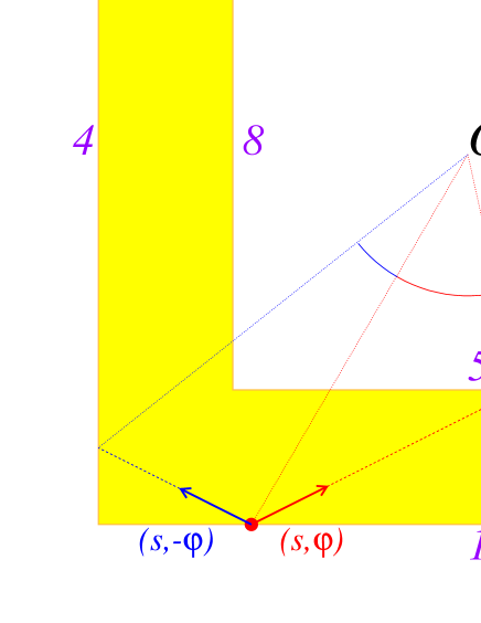
Figure 1: (Colour online) Billiard table for $l_{1}/l_{2}=\pi/2$. A portion of a trajectory of a particle with initial condition $(s,\varphi)$, evolving under $B_{\varphi}^{t}$ with $t\geq 0$, is shown; $(s,-\varphi)$ is the ”time reversed” initial condition.

2 The model.

2.1 Description of the billiard table

We consider the dynamics of a classical point particle in a doubly connected rational polygonal billiard. The billiard table, shown in figure 1, is delimited by two concentric squares with parallel sides of length $l_{1}$ and $l_{2}$ ($l_{1}>l_{2}$). The particle moves freely inside the billiard, colliding elastically with the boundary; the (preserved) modulus of the velocity is taken equal to $1$. The accessible phase space is 3-dimensional and the representative point is $(x,y,\theta)$: $(x,y)$ are the Cartesian coordinates of the particles and $\theta$ is the angle of the velocity, measured counterclockwise from the positive $x$-axis. The billiard flow, denoted by $T^{t}$, preserves the Lebesgue measure ${\rm d}x{\rm d}y{\rm d}\theta/(2\pi(l_{1}^{2}-l_{2}^{2}))$.

We may also consider the discrete time dynamics, induced by successive collisions. Each collision point can be parametrized by a coordinate $s$ along the boundary and an angle $\varphi$, between the outgoing direction and the inner normal to the boundary; we take $\varphi$ positive if the outgoing velocity is given by a counterclockwise rotation to the inner normal. By denoting $L=2(l_{1}+l_{2})$, the arclength $s\in[-L,L)$ takes the value $s=-L$ in the left corner of side 1 and increases by moving counterclockwise along the sides of the billiard, labeled by increasing numbers (see figure 1). The corresponding phase space is called ${\mathcal{M}}=\{(s,\varphi);s\in[-L,L),\varphi\in[-\pi/2,\pi/2)\}$ and the Birkhoff-Poincaré map is denoted by $B^{t}$ ($t\in{{\mathbb{Z}}}$); the map $B^{t}$ preserves the measure ${\rm d}\Omega(z)=\cos\varphi{\rm d}\varphi\;{\rm d}s\;/(4L)$ on ${\mathcal{M}}$.

Dynamics on such billiards is strongly influenced by number–theoretical properties of $l_{2}/l_{1}$ and of $\tan\varphi$; in particular we may distinguish three classes [24]: $(i)$ class 1: $l_{2}/l_{1},\tan\varphi\in{\mathbb{Q}}$; $(ii)$ class 2: $l_{2}/l_{1}\in{\mathbb{Q}}$, $\tan\varphi\in{{\mathbb{R}}-{\mathbb{Q}}}$; $(iii)$ class 3: $l_{2}/l_{1}\in{\mathbb{R}}-{\mathbb{Q}}$, $\tan\varphi\in{{\mathbb{R}}-{\mathbb{Q}}}$. In this paper we restrict to class 3.

2.2 Review on basic spectral properties

As all the internal angles are rational multiples of $\pi$, it is fairly easy to realize that the flow on the global phase space, or the mapping $B^{t}$ on ${\mathcal{M}}$, can never be ergodic. However $T^{t}$ can be decomposed into the one-parameter family of directional flows at fixed $\theta$, $T^{t}_{\theta}$, whose dynamics is not trivial: in particular, $T^{t}_{\theta}$ is ergodic for almost all $\theta\in[0,\pi/2)$ and never mixing [20, 21]. It is believed that the weak-mixing property should be enjoyed by a “generic” subset of directional flows, and numerical evidences for class 3 are provided in [24].

Analogously to the billiard flow, the map $B^{t}$ can be decomposed into a one-parameter family of components $B^{t}_{\varphi}$ along the fixed direction $\varphi$ (with $0\leq\varphi\leq\pi/2$). Once the initial outgoing angle is set, only the angles $\pm\varphi,\pm(\frac{\pi}{2}-\varphi)$ can be met along the trajectory, so the phase space for any fixed foliation, i.e. ${\mathcal{M}}_{\varphi}$, is a fourfold replica of $[-L,L)$: its points are denoted by $z=(s,\pm\varphi_{j})$ with $\varphi_{j}=\varphi-j\pi/2$ and $j=0,1$. The phase average of an observable $f:{\mathcal{M}}_{\varphi}\to{\mathbb{C}}$ can be written explicitly as:

$$\int_{{\mathcal{M}}_{\varphi}}{\rm d}\Omega(z)\;f(z)=\frac{1}{8L}\int_{-L}^{L}{\rm d}s\;\sum_{j=0}^{1}\cos{\varphi_{j}}\left\{f(s,{\varphi_{j}})+f(s,-{\varphi_{j}})\right\}.$$ (1)

Spectral properties of the system can be formulated in terms of the asymptotic behaviour of the correlation functions.

Ergodicity of $B^{t}_{\varphi}$ implies that the time-averaged correlation function of a generic (real) phase function $f:{\mathcal{M}}_{\varphi}\to{\mathbb{R}}$:

$$C^{time}_{f}(t,z)=\lim_{T\to+\infty}\frac{1}{2T}\sum_{t^{\prime}=-T}^{T-1}f(B^{t^{\prime}+t}_{\varphi}z)f(B^{t^{\prime}}_{\varphi}z),$$ (2)

and the phase-averaged correlation function:

$$C^{ph}_{f}(t)=\langle f|U^{t}f\rangle=\int_{{\mathcal{M}}_{\varphi}}{\rm d}\Omega(z)\;f(B_{\varphi}^{t}z)f(z),$$ (3)

coincide for $\Omega$-almost every $z\in{\mathcal{M}}_{\varphi}$. The unitary operator $U$ in (3) is the Koopman operator, associated to the map $B^{t}_{\varphi}$.

As directional flows or mappings are not mixing, correlation functions (of zero mean observables) do not decay to zero in the asymptotic limit; while the (conjectured) weak-mixing property guarantees that integrated correlations:

$$C^{int}_{f}(t)=\frac{1}{t}\sum_{s=0}^{t-1}\left|C^{ph}_{f}(s)\right|^{2}$$ (4)

vanish as $t\to\infty$. Phase-averaged correlation function and integrated correlation function of the angle $\xi$, spanned by the radius vector of a particle between two successive collision points, are shown in figure 2(a) for a generic billiard belonging to class 3: while $C^{ph}(t)\not\to 0$ (upper line), $C^{int}_{f}(t)$ decays to zero polynomially (lower line).

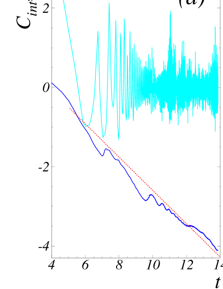
Figure 2: (Colour online) (a) Phase averaged (upper line) and integrated (lower) correlation functions of the angle $\xi$, spanned by the radius vector, as a function of time $t$ (measured in numbers of collisions). The billiard table belongs to class 3 with parameters: $l_{1}/l_{2}=\pi/2$ and $\tan\varphi=\pi/4$. The dotted line, which fits $C^{int}(t)$, has a slope equal to $-D_{2}$. (b) Estimates of generalized dimensions $D_{1}$ (empty symbols) and $D_{2}$ (full symbols) of the spectral measure, associated to $\xi$, for the same parameters. The dimension estimates are given by the slopes of straight lines: $D_{1}=0.69\pm 0.01$ and $D_{2}=0.42\pm 0.02$. Details are explained in section 6.

By using the spectral decomposition of the Koopman operator $U$, we may rewrite (3) as

$$C^{ph}_{f}(t)=\frac{1}{2\pi}\int_{-\pi}^{\pi}{\rm d}\mu_{f}(\theta)e^{i\theta t},$$ (5)

which provides a direct link between the autocorrelation function of an observable $f$ and the associated spectral measure. If (in the complement of constant functions) the spectral measure is absolutely continuous, the system is mixing. On the other side, weak mixing is equivalent to an empty point spectrum, apart from the eigenvalue 1. Therefore, the weak mixing property, without the stronger mixing property, entails the presence of a singular continuous component of the spectrum of the Koopman operator.

Owing to the presence of a non empty point spectra, weakly mixing property is ruled out in the almost integrable cases, namely for $l_{1}/l_{2}\in{{\mathbb{Q}}}$ (class 1 and class 2); we will not consider such cases in the present work.

In [24], the occurrence of a singular continuous component of the spectrum in billiards of class 3 was inferred by looking at scaling properties of the spectral measure, obtained by finer and finer numerical inversion of (5). In particular a multifractal analysis yields a nontrivial spectrum of generalized dimensions, with a Hausdorff dimension $D_{1}$ less than 1 and a correlation dimension $D_{2}$ which rules the power-law decay of integrated correlations [31, 32]. An example is shown in figure 2(b), for the spectral measure associated to the angle $\xi$. As we will show in following sections, the local scaling properties of the spectral measure are even more relevant in connection with transport properties. For billiards in class 3, a nontrivial scaling of the spectral peaks near the zero frequency is found (see figure 4(b)), in opposition to the almost integrable case, in which a non empty pure point spectrum is marked by not scaling deltalike peaks at different resolutions [24].

3 Higher order statistics

3.1 Dynamical quantities and spectral analysis

The dynamics inside the billiard table in figure 1 is equivalent to the dynamics of the particles in a two-dimensional infinite periodic lattice with square obstacles, i.e. in a generalized Lorentz gas, recently examined in [12, 13, 14, 16, 28]. The unfolded system is obtained by reflecting the elementary cell and the segment of a trajectory at each collision point with the external square. Instead of considering particle diffusion along the channels of the extended system, we examine the transport generated by billiard trajectories revolving around the inner square obstacle.

For this purpose, the natural observable is the angle $\xi(z)$, spanned by the radius vector, joining the center of the billiard $O$ with the collision point $z$, when the particle is moving from $z$ to $B_{\varphi}z$; it is assumed positive when counterclockwise. The total angle accumulated by a single particle up to time $t$ is:

$$\Xi(z,t)=\sum_{s=0}^{t-1}\xi(B_{\varphi}^{s}z);$$ (6)

$\Xi(z,t)/(2\pi)$ gives the number of revolutions completed by a trajectory up to the time $t$.

In [24] the 2-nd order moment $\sigma^{2}(t)$ of $\Xi(z,t)$, namely the r.m.s. number of revolutions, was examined; for generical values of the parameters in class 3, an “anomalous diffusion” was found, marked by an algebraic growth of $\sigma^{2}$ in time with an exponent ranging between 1 (normal diffusion) and 2 (ballistic transport); this exponent has shown to be related to the zero-frequency scaling index of the density power spectrum associated to the observable $\xi(z)$. In this paper we extend the analysis to moments of arbitrary order.

Since $\xi(B_{\varphi}^{t}z)$ is a “power signal”, i.e. $\{\xi(B_{\varphi}^{t}z)\}_{t\in{\mathbb{Z}}}\not\in\ell^{2}({\mathbb{Z}})$, as a function of time $t$, but $W=\lim_{T\to\infty}\frac{1}{2T}\sum_{t=-T}^{T-1}\xi^{2}(B_{\varphi}^{t}z)\equiv C^{time}_{\xi}(0;z)<+\infty$, we analyse the trajectory of a particle on a finite time interval: $-T\leq t\leq T$ (with $T$ positive integer, i.e. $T\in{{\mathbb{N}}_{+}}$). Spectral analysis will involve Fourier transform of the signal $\xi(B_{\varphi}^{t}z)$ on finite portions of trajectories.

Hence we call $\hat{\xi}_{T}$ the partial sum of the Fourier series of $\xi(B_{\varphi}^{t}z)$:

$$\hat{\xi}_{T}(\theta;z)=\left({k}_{T}\ast\hat{\xi}\right)(\theta;z)=\sum_{t=-T}^{T-1}\xi(B_{\varphi}^{t}z)e^{-it\theta}=\rho_{T}(\theta;z)e^{i\phi_{T}(\theta;z)},$$ (7)

where $\ast$ denotes convolution and ${k}_{T}(x)=\sum_{t=-T}^{T-1}e^{-ixt}=e^{i\frac{x}{2}}\left(\frac{\sin Tx}{\sin\frac{x}{2}}\right)$. The upper limit of the sum in (7) is determined by the fact that $\xi(B_{\varphi}^{T}z)$ is not defined.

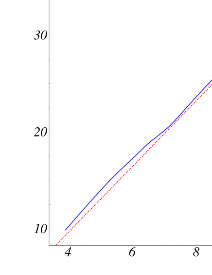
Figure 3: (Colour online) Fourth order moment of $\Xi(z,t)$ vs time in logarithmic scales, for the same data of figure 4. The slope of the straight line (= 3.4) is given by the theoretical prediction (37) with $n=4$ and ${\bar{\alpha}}(0)=0.3$.

$\left\{\hat{\xi}_{T}(\theta;z)\right\}_{T\in{{\mathbb{N}}_{+}}}$ is a sequence of continuous, bounded and periodic complex function of the frequency $\theta\in{\mathbb{T}}$; ${\mathbb{T}}={\mathbb{R}}/(2\pi{\mathbb{Z}})$ denotes the 1-dimensional torus. As $\xi(B_{\varphi}^{t}z)\not\to 0$ for $t\to\infty$, the limit $T\to\infty$ of the sequence of partial sums may not be a function in ordinary sense; as $|\xi(t;z)|\leq A$ $\forall t\in{\mathbb{Z}}$ and $0<A<\pi$, from the theory of Fouries series, it follows that $\left\{\hat{\xi}_{T}(\theta;z)\right\}_{T\in{{\mathbb{N}}_{+}}}$ converges weakly for $T\to\infty$ to a tempered distribution of period ${\mathbb{T}}$.

Since $\xi$ is a real-valued function, $\hat{\xi}_{T}^{*}(\theta;z)=\hat{\xi}_{T}(-\theta;z)$ and the absolute value and the phase of $\hat{\xi}_{T}$ are respectively even and odd functions of $\theta$ (mod $2\pi$) :

$$\rho_{T}(-\theta;z)=\rho_{T}(\theta;z)=\rho_{T}(|\theta|;z)$$ (8)

$$\phi_{T}(-\theta;z)=-\phi_{T}(\theta;z).$$ (9)

In particular $\hat{\xi}_{T}(0;z)=\rho_{T}(0;z)$, $\phi_{T}(0;z)=0$; while, from periodicity and from (9), it follows that $\phi_{T}(-\pi;z)=\phi_{T}(\pi;z)=0$.

By looking at forward trajectories starting at $(s,\varphi)$ and their time reversal, generated by the “backward” (inverse) operator $B_{\varphi}^{-1}$ on $(s,-\varphi)$, we can verify that the following identity holds:

$$\xi(B_{\varphi}^{t}(s,-\varphi))=-\xi(B_{\varphi}^{-t-1}(s,\varphi)).$$ (10)

This identity induces the following property of the partial sums:

$$\hat{\xi}_{T}(\theta;(s,-\varphi))=-e^{i\theta}\hat{\xi}_{T}^{*}(\theta;(s,\varphi)),$$ (11)

which is equivalent to $\rho_{T}(\theta;(s,-\varphi))=\rho_{T}(\theta;(s,\varphi))$ and $\phi_{T}(\theta;(s,-\varphi))=\theta+\pi-\phi_{T}(\theta;(s,\varphi))$ (mod ($2\pi$)).

3.2 Higher order moments and correlations

To get a more detailed picture of anomalous transport, we introduce the higher order statistics of $\Xi(z,t)$ and higher order spectral analysis of the phase variable $\xi(z)$.

While, from the numerical point of view, we may take arbitrarily real powers of the diffusing variable $|\Xi(z,t)|$, in the theoretical analysis of sections 3, 4 and 5, we restrict to integer order moments of $\Xi(z,t)$. Integer order moments can be expressed in terms of multiple-time correlation functions, related to higher order spectra.

The $n$-th order moment is given by:

$$\sigma^{(n)}(t)=\int_{{\mathcal{M}}_{\varphi}}{{\rm d}}\Omega(z)\Xi^{n}(z,t)\qquad\quad n\geq 2.$$ (12)

The occurrence of anomalous diffusion, previously found for $\sigma^{2}(t)$ [24], is confirmed for moments of arbitrary orders; in figure 3 the fourth-order moment is shown, as an example. The crucial issue is to get an estimate for the exponents of the algebraic growth in time of integer moments.

By a generalization of (3), we introduce a multiple-time phase-averaged correlation function of the observable $\xi$, which depends on $(n-1)$ time intervals:

$$C^{ph}_{\xi}(\vec{t})=\int_{{\mathcal{M}}_{\varphi}}{\rm d}\Omega(z)\;\xi(z)\left(\prod_{l=0}^{n-1}\xi(B_{\varphi}^{t_{l}}z)\right),\qquad\vec{t}=(t_{1},t_{2},\cdots,t_{n-1})\in{\mathbb{Z}}^{n-1}.$$ (13)

The $n$-th moment $\sigma^{(n)}(t)$ can be expressed as a function of $C^{ph}_{\xi}(\vec{t})$:

$$\sigma^{(n)}(t) = \sum_{t_{0}=0}^{t-1}\sum_{t_{1}=0}^{t-1}\cdots\sum_{t_{n-1}=0}^{t-1}\int_{{\mathcal{M}}_{\varphi}}{\rm d}\Omega(z)\;\xi(B_{\varphi}^{t_{0}}z)\xi(B_{\varphi}^{t_{1}}z)\xi(B_{\varphi}^{t_{2}}z)\cdots\xi(B_{\varphi}^{t_{n-1}}z)$$ (14)

$$= \sum_{t_{0}=0}^{t-1}\sum_{t_{1}=0}^{t-1}\cdots\sum_{t_{n-1}=0}^{t-1}C^{ph}_{\xi}(\vec{t}-t_{0}\vec{I}),$$

where $\vec{I}$ is the vector with all entries equal to 1; note that the $n$-th order moment is related to a $(n-1)$-point correlation function.

4 Higher order spectra analysis.

4.1 Multi-dimensional Wiener-Khinchin theorem

The $(n-1)$-point correlation can be expressed in terms of a $(n-1)$-dimensional inverse Fourier transform of the $(n-1)$-th order spectral density distribution function (polyspectrum) on ${\mathbb{T}}^{n-1}$ [34, 35]:

$$C^{ph}_{\xi}(\vec{t}\;)=\frac{1}{(2\pi)^{n-1}}\int_{{{\mathbb{T}}^{n-1}}}{\rm{\bf d}}\vec{\theta}\;m_{\xi}(\vec{\theta})e^{i\vec{\theta}\cdot\vec{t}};$$ (15)

${\mathbb{T}}^{n-1}$ is the $(n-1)$-dimensional torus, i.e. the Cartesian product of $(n-1)$ tori ${\mathbb{T}}\times{\mathbb{T}}\cdots\times{\mathbb{T}}$ and $\vec{\theta}=(\theta_{1},\theta_{2},\cdots,\theta_{n-1})\in{\mathbb{T}}^{n-1}$. Equation (15) is a formal generalization of the Wiener-Khinchin Theorem to the multi-dimensional case. However, since for $n>2$, $C^{ph}_{\xi}(\vec{t}\;)$ is not a positive definite function, according to Bochner’s Theorem, $m_{\xi}(\vec{\theta})$ is not a positive distribution and $m_{\xi}(\vec{\theta}){\rm{\bf d}}\vec{\theta}$ cannot be interpreted as a probability measure on ${\mathbb{T}}^{n-1}$ [36, 37].

An alternative version of the theorem involves the time-averaged correlation function:

$$C^{time}_{\xi}(\vec{t};z) \equiv\lim_{T\to\infty}\frac{1}{2T}\sum_{t=-T}^{T-1}\xi(B_{\varphi}^{t}z)\left(\prod_{l=1}^{n}\xi(B_{\varphi}^{t+t_{l}}z)\right)$$ (16)

$$=\frac{1}{(2\pi)^{n}}\int_{{{\mathbb{T}}^{n-1}}}{\rm{\bf d}}\vec{\theta}\;s_{\xi}(\vec{\theta};z)e^{i\vec{\theta}\cdot\vec{t}},$$ (17)

with

$$m_{\xi}(\vec{\theta})=\int_{{\mathcal{M}}_{\varphi}}{\rm d}\Omega(z)s_{\xi}(\vec{\theta};z).$$ (18)

If the system is ergodic, $s_{\xi}(\vec{\theta};z)=m_{\xi}(\vec{\theta})$, for $\Omega$-almost every $z\in{\mathcal{M}}_{\varphi}$.

4.2 Polyspectra

We may obtain $m_{\xi}(\vec{\theta})$ in terms of partial sums of the Fourier series of $\xi(B_{\varphi}^{t}z)$.

Firstly, we derive $s_{\xi}(\vec{\theta};z)$ from (17). Since we consider the trajectory of a particle on a finite time interval, each signal $\xi(B_{\varphi}^{t+t_{l}}z)$ in (16) is substituted by $\chi_{{\mathcal{I}}_{T}}(t+t_{l})\cdot\xi(B_{\varphi}^{t+t_{l}}z)$, where $\chi_{{\mathcal{I}}_{T}}$ is the characteristic function of the interval of integers ${{\mathcal{I}}_{T}}\equiv\{t\in{\mathbb{Z}};-T\leq t\leq T-1\}$.

The square window of the signal is expressed by the Fourier transform

$${\chi}_{{\mathcal{I}}_{T}}(t)\xi(B^{t}z)=\frac{1}{2\pi}\int_{-\pi}^{\pi}{\rm d}\theta\;\hat{\xi}_{T}(\theta;z)e^{i\theta t},$$ (19)

which is obtained by the Convolution Theorem from (7).

The polyspectra $s_{\xi}(\vec{\theta};z)$ (and thus $m_{\xi}(\vec{\theta})$) is given as a limit of a sequence of functions $\{s_{T,\xi}(\vec{\theta};z)\}_{T\in{{\mathbb{N}}_{+}}}$, which converges to $s_{\xi}(\vec{\theta};z)$ in a weak sense:

$$s_{\xi}(\vec{\theta};z)=\lim_{T\to\infty}s_{T,\xi}(\vec{\theta};z)\quad{\rm weakly}.$$

By inverting (17) and substituting (19), we get:

$$s_{T,\xi}(\vec{\theta};z)=\frac{1}{2T}\sum_{t=-T}^{T-1}\sum_{t_{1}=-T-t}^{T-t-1}\cdots\sum_{t_{n-1}=-T-t}^{T-t-1}e^{-i\vec{\theta}\cdot\vec{t}}\chi_{{\mathcal{I}}_{T}}(t)\xi(B^{t}z)\prod_{l=1}^{n-1}\chi_{{\mathcal{I}}_{T}}(t+t_{l})\xi(B^{t+t_{l}}z)$$

$$\quad\qquad\;\;=\frac{1}{2T(2\pi)^{n}}\int_{{\mathbb{T}}}{\rm d}\theta\ \int_{{\mathbb{T}}^{n-1}}{\rm{\bf d}}\vec{\theta}^{\prime}\hat{\xi}_{T}(\theta;z)k^{*}_{T}(\theta+\Theta(\vec{\theta}))\prod_{l=1}^{n-1}\hat{\xi}_{T}(\theta^{\prime}_{l};z)k_{T}(\theta_{l}-\theta^{\prime}_{l}),$$

where $\Theta(\vec{\theta})=\sum_{l=1}^{n-1}\theta_{l}$. By using that $k_{T}(x)$ (and $k^{*}_{T}(x)$) is an approximate identity, i.e. $\lim_{T\to\infty}\int_{{\mathbb{T}}}{\rm d}\theta k_{T}(\theta-\theta^{\prime})f(\theta)=2\pi f(\theta^{\prime})$ for all continuous functions $f$ on ${\mathbb{T}}$, the final expression of $s_{\xi}(\vec{\theta};z)$ is obtained:

$$s_{\xi}(\vec{\theta};z)=\lim_{T\to\infty}\frac{1}{2T}\left(\prod_{j=1}^{n-1}\hat{\xi}_{T}(\theta_{j};z)\right)\hat{\xi}^{*}_{T}\left(\Theta(\vec{\theta});z\right).$$ (20)

$m_{\xi}(\vec{\theta})$ is derived by applying phase averages (18) to both sides of (20). The result is consistent with analogous formulas in [34, 38].

We introduce the notation: $\Gamma_{T}(\vec{\theta};{z_{s,l}})=\prod_{j=1}^{n-1}\rho_{T}(\theta_{j};{z_{s,l}})$ and $\Phi_{T}(\vec{\theta};{z_{s,l}})=\sum_{j=1}^{n-1}\phi_{T}(\theta_{j};{z_{s,l}})$, with ${z_{s,l}}=(s,\varphi_{l})$ and $\varphi_{l}=\varphi-l\pi/2$ ($l=0,1$).

By evaluating the phase average with (1) and by making use of the property (11), we get:

$$m_{\xi}(\vec{\theta})=\lim_{T\to\infty}m_{T,\xi}(\vec{\theta})\quad{\rm weakly}$$

$$m_{T,\xi}(\vec{\theta})=\frac{1}{4L}\int_{-L}^{L}{\rm d}s\sum_{l=0}^{1}\cos{\varphi_{l}}\;\cdot M_{T,\xi}(\vec{\theta};{z_{s,l}});$$ (21)

for $n$ odd integer:

$$M_{T,\xi}(\vec{\theta};{z_{s,l}})=\frac{i}{2T}\Gamma_{T}(\vec{\theta};{z_{s,l}})\rho_{T}(\Theta(\vec{\theta});{z_{s,l}})\sin\left(\Phi_{T}(\vec{\theta};{z_{s,l}})-\phi_{T}(\Theta(\vec{\theta});{z_{s,l}})\right);$$ (22)

for $n$ even integer:

$$M_{T,\xi}(\vec{\theta};{z_{s,l}})=\frac{1}{2T}\Gamma_{T}(\vec{\theta};{z_{s,l}})\rho_{T}(\Theta(\vec{\theta});{z_{s,l}})\cos\left(\Phi_{T}(\vec{\theta};{z_{s,l}})-\phi_{T}(\Theta(\vec{\theta});{z_{s,l}})\right).$$ (23)

Explicit formulas for the first few orders are given in A.

Higher order spectra $m_{\xi}(\vec{\theta})$ possess different symmetry properties.

From (20) and since $\hat{\xi}^{*}_{T}(\theta;z)=\hat{\xi}_{T}(-\theta;z)$, a conjugate symmetry property holds for $m_{\xi}(\vec{\theta})$:

$$m_{\xi}^{*}(\vec{\theta})=m_{\xi}(-\vec{\theta});$$ (24)

this condition guarantees the reality of multiple-time correlation $C_{\xi}^{ph}(\vec{t})$, expressed by (15).

In particular, from (22), (23), (8) and (9), we get:

$$m_{\xi}(-\vec{\theta})=-m_{\xi}(\vec{\theta})\qquad\qquad {\rm for}\;{\rm odd}\;n$$ (25)

$$m_{\xi}(-\vec{\theta})=m_{\xi}(\vec{\theta})\qquad\qquad {\rm for}\;{\rm even}\;n.$$ (26)

For odd $n$ (25) entails that the multiple integral of $m_{\xi}(\vec{\theta})$ on ${\mathbb{T}}^{n-1}$ is null, because the contributions of hyperoctants associated to $\vec{\theta}$ and $-\vec{\theta}$ cancel each other. For even $n$ instead, owing to (26), these contributions are equal and the integration domain can be reduced from $2^{n-1}$ hyperoctants to $2^{n-2}$ hyperoctants.

The multiple-time correlation function $C^{ph}_{\xi}(\vec{t})$ posseses further symmetry properties, which reflect to symmetries of $m_{\xi}(\vec{\theta})$ and allow to further reduce the integration domain in (15) to the “so-called” principal domain [27, 39]. These symmetry conditions are reviewed in A.1 for the bispectrum and trispectrum, i.e. $n=3$ and $n=4$.

4.3 Single frequency case: small frequency asymptotics of the spectral measure

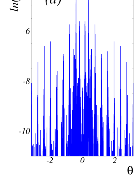
Figure 4: (Colour online) (a) Numerical reconstruction of the density power spectrum $m_{\xi}(\theta)$ associated to the angle $\xi$ with a resolution $\Delta\theta=2\pi/2^{14}$, for $l_{1}/l_{2}=\pi/2$ and $\tan\varphi=\pi/4$. (b) Mass contained in small intervals of radius $\delta$ centered at $0$ vs $\delta$. The slope of the straight line gives the Hölder exponent at $\theta=0$, i.e. ${\bar{\alpha}}(0)=0.30$. Different symbols refer to different resolutions of $m_{\xi}(\theta)$, as explained in section 6.

In section 5 we make use of the asymptotic behaviour of polyspectra for vanishing frequencies. Since (20) and (4.2) are expressed in terms of products of one-variable functions, in this section we focus on the single frequency case, namely $n=2$.

The correlation functions (15) and (17) are expressed by 1-dimensional integrals; $s_{\xi}(\theta;z)$ is the density power spectrum of the signal, obtained by a weak limit of the sequence of functions $\{s_{T,\xi}(\theta;z\}_{T\in{{\mathbb{N}}_{+}}}$:

$$s_{T,\xi}(\theta;z)=\frac{1}{2T}\hat{\xi}_{T}(\theta;z)\;\hat{\xi}^{*}_{T}(\theta;z)=\frac{1}{2T}\rho_{T}^{2}(\theta;z).$$ (27)

By comparing (15), for $n=2$, with (5) we have

$${\rm d}\mu_{\xi}(\theta)=m_{\xi}(\theta){\rm d}\theta,$$ (28)

which has to be interpreted in a strict distributional sense, as in our case $m_{\xi}(\theta)$ will be a singular object. In billiards of class 3, as explained in section 2.2, the absence of mixing excludes occurrence of purely absolute continuous spectrum and implies that the correlations do not decay to zero as $t\to\infty$; therefore, owing to Riemann-Lebesgue Lemma, $m_{\xi}(\theta)$ is not an integrable function of $\theta\in{\mathbb{T}}$.

In [24] it was pointed out that the singularity of the measure at $\theta=0$ is essential in order to get an anomalous second moment of the transporting variable; in particular the indices that quantify such singularities are the critical Hölder exponents ${\bar{\alpha}}(\theta)$, which are defined for each point $\theta$ in the support of the measure as

$$\limsup_{\delta\to 0}\mu_{\xi}({\mathcal{I}}_{\delta}(\theta))\cdot\delta^{-\alpha}=\left\{\begin{array}[]{ll}0&\alpha<{\bar{\alpha}}(\theta)\\ \infty&\alpha>{\bar{\alpha}}(\theta)\end{array}\right.,$$ (29)

where ${\mathcal{I}}_{\delta}(\theta)=[\theta-\delta,\theta+\delta]$ is an interval of width $2\delta$, centered in $\theta$. The measure is uniformly ${\bar{\alpha}}$-Hölder continuous (U${\bar{\alpha}}$H) in an interval ${\mathcal{I}}_{\Delta}(\tilde{\theta})$, centered in a particular point $\tilde{\theta}$, if a positive constant $c$ exists such that the mass $\mu_{\xi}({\mathcal{I}}_{\delta}(\theta))\leq c\delta^{{\bar{\alpha}}(\tilde{\theta})}$ for every interval ${\mathcal{I}}_{\delta}(\theta)\subset{\mathcal{I}}_{\Delta}(\tilde{\theta})$.

Smaller values of ${\bar{\alpha}}$ correspond to stronger singularities of the spectral measure. The more interesting case is when $0\leq{\bar{\alpha}}\leq 1$; in the following, we will consider ${\bar{\alpha}}(\tilde{\theta})$ varying within this range. The values ${\bar{\alpha}}=0$ and ${\bar{\alpha}}\geq 1$ correspond to a discrete and absolutely continuous component of the spectral measure, respectively; if ${\bar{\alpha}}(\tilde{\theta})=0$, $\mu_{\xi}(\{\tilde{\theta}\})>0$ and if ${\bar{\alpha}}(\tilde{\theta})\geq 1$, the measure is continuous and differentiable in ${\mathcal{I}}_{\Delta}(\tilde{\theta})$ and the derivative $m_{\xi}(\theta)$, being an integrable function on ${\mathcal{I}}_{\Delta}(\tilde{\theta})$, is the density of the measure, with respect to Lebesgue measure. According to numerical approximations of the spectral measure, billiards belonging to class 3 are characterized by values of ${\bar{\alpha}}$ in the range $0<{\bar{\alpha}}<1$; in figure 4 a typical case is shown, in which ${\bar{\alpha}}(0)=0.3$. This is consistent with the presence of a singular continuous component of the spectrum; however, an exponent ${\bar{\alpha}}\in(0,1)$ is not a sufficient condition to have either a continuous [24] or singular continuous part [25] of the measure.

In section 5 we will use a relationship which connects the Hölder exponent of the measure at some point $\tilde{\theta}$ to the asymptotic behaviour as $T\to+\infty$ of the sequence $\{m_{T,\xi}(\theta)\}_{T\in{{\mathbb{N}}_{+}}}$; it is based on the equality $m_{T,\xi}(\theta)=\frac{1}{2\pi}\int_{{\mathbb{T}}}{\rm d}\mu_{\xi}(\theta^{\prime})K_{T}(\theta-\theta^{\prime})$ with $K_{T}(x)=({\sin Tx}/{\sin(x/2)})^{2}/2T$. This relationship is derived in [25] and reviewed in B.

If the measure is U${\bar{\alpha}}$H in an interval ${\mathcal{I}}_{\Delta}(\tilde{\theta})$, then there exist a positive constant $D$ and $\bar{T}=\bar{T}(\Delta,\theta)$ such that for $T>\bar{T}$:

$$m_{T,\xi}(\theta)\leq DT^{1-{\bar{\alpha}}(\tilde{\theta})}\qquad{\rm uniformly\;for}\;\theta\in{\mathcal{I}}_{\Delta}(\tilde{\theta}).$$ (30)

As we are dealing with an ergodic system, the bound (30) holds also for $s_{T,\xi}(\theta;z)$, for $\Omega$-a.e. $z\in{\mathcal{M}}_{\varphi}$, because the dependence on $z$ in (18) is actually missing.

Consequently, it follows from (27) that, for $\Omega$-a.e. $z$, the sequence of functions $\rho_{T}(\theta;z)$ as $T\to+\infty$ is bounded by:

$$\rho_{T}(\theta;z)\leq CT^{1-\frac{{\bar{\alpha}}(\tilde{\theta})}{2}}\qquad{\rm for}\;\theta\in{\mathcal{I}}_{\Delta}(\tilde{\theta}),\;\;{\rm with}\;\;C>0;$$ (31)

in particular, for instance, if $\tilde{\theta}=0$ and $\Delta=2{\pi}/{\bar{T}}$ (with $\bar{T}\geq 2$), (31) holds in every interval ${\mathcal{I}}_{\delta}(\theta)$ with $\delta\leq 2{\pi}/{T}$.

5 Analytic estimate for the moments’ scaling function

An accurate study of moments’ asymptotic behaviour at large times is the central point of the present paper. The moments’ scaling function $\gamma(n)$ is defined as the real number $\gamma(n)$ such that the discrete Mellin transform:

$$I^{(n)}(\beta)=\sum_{t=1}^{+\infty}\frac{1}{t^{1+\beta}}\sigma^{(n)}(t),$$ (32)

converges for $\beta>\gamma(n)$ and diverges for $\beta<\gamma(n)$. This definition of $\gamma(n)$, respect to other definitions based on the asymptotic behaviour of $\sigma^{(n)}(t)$ as $t\to\infty$, has the advantage that it does not take into account of possible subdominant contributions to the transport process.

The moments’ scaling function may be written as $\gamma(n)=\nu(n)n$. Normal transport and weak anomalous transport fall in the category with $\nu(n)=\nu_{0}=const.$ with $\nu_{0}=1/2$ and $\nu_{0}\not=1/2$, respectively; at long times, the distribution of $\Xi(z,t)$ relaxes to a self-similar function, which is a Gaussian distribution when $\nu_{0}=1/2$. Strong anomalous transport corresponds to the case where the distribution of $\Xi$ does not collapse to a self-similar form, multiple scales exist and a phase transition is observed, marked by a piecewise linear function $\nu(n)$ [29, 33].

For even moments of integer order ( $n\geq 2$), we obtain an analytic relationship, linking the scaling function $\gamma(n)$ with Hölder exponent at $\theta=0$ of the spectral measure associated to $\xi(z)$. This relation extends to higher order moments the formula found in [24] for the exponent $\gamma(2)$ of the 2-nd moment.

By substituting (15) into (14), the moment of order $n$ is expressed by the following multiple integral over the $(n-1)$-dimensional torus ${{\mathbb{T}}^{n-1}}$:

$$\sigma^{(n)}(t)=\frac{1}{(2\pi)^{n-1}}\int_{{{\mathbb{T}}^{n-1}}}{\rm{\bf d}}\vec{\theta}\;m_{\xi}(\vec{\theta}\;)D_{t}\left(\Theta(\vec{\theta})\right)\prod_{j=1}^{n-1}D_{t}(\theta_{j}),$$ (33)

where $D_{t}(x)$ denotes the kernel:

$$D_{t}(x)=e^{-\frac{i}{2}x(t-1)}\sum_{n=0}^{t-1}e^{inx}=\frac{\sin\left(\frac{x}{2}t\right)}{\sin\left(\frac{x}{2}\right)}.$$ (34)

The conjungate symmetry property (24) of the polyspectrum guarantees that the expression (33) is real. Moreover, since $D_{t}(x)$ is an even function of $x$, the parity transformation property of the integrand in (33) is determined by $m_{\xi}(\vec{\theta})$. From (25), it follows that all moments of odd order are null. This is consistent with the fact that the angle $\Xi(z,t)$, accumulated by a single particle, may assume positive or negative values; hence, in C, odd order moments of $|\Xi(z,t)|$ are taken into account.

For even $n$, owing to symmetry (26), the integration domain of (33) can be reduced to half of the $(n-1)$-dimensional hyperoctans.

By substituting (33) into (32), we get:

$$I^{(n)}(\beta)=\frac{2}{(2\pi)^{n-1}}\sum_{l=1}^{2^{n-2}}I_{l}^{(n)}(\beta)$$

$$I^{(n)}_{l}(\beta)=\int_{{{\mathbb{L}}}_{l}^{n-1}}{\rm{\bf d}}\;\vec{\theta}\;m_{\xi}(\vec{\theta})S(\beta,\vec{\theta})=\lim_{T\to\infty}\int_{{{\mathbb{L}}}_{l}^{n-1}}{\rm{\bf d}}\;\vec{\theta}\;m_{T,\xi}(\vec{\theta})S_{T}(\beta,\vec{\theta})$$

$$S_{T}(\beta,\vec{\theta})=\sum_{t=1}^{T}\frac{1}{t^{1+\beta}}D_{t}\left(\Theta(\vec{\theta})\right)\prod_{j=1}^{n-1}D_{t}(\theta_{j})\qquad\quad S(\beta,\vec{\theta})=\lim_{T\to\infty}S_{T}(\beta,\vec{\theta})$$

The integration domains ${\mathbb{L}}_{l}^{n-1}$ in (5) are Cartesian products of $(n-1)$ half tori, ${\mathbb{T}}_{+}=[0,\pi]$ or ${\mathbb{T}}_{-}=]-\pi,0]$. For instance for $n=4$, ${\mathbb{L}}_{l}^{3}$ are the following octants: ${\mathbb{L}}_{1}^{3}={\mathbb{T}}_{+}\times{\mathbb{T}}_{+}\times{\mathbb{T}}_{+}$, ${\mathbb{L}}_{2}^{3}={\mathbb{T}}_{+}\times{\mathbb{T}}_{+}\times{\mathbb{T}}_{-}$, ${\mathbb{L}}_{3}^{3}={\mathbb{T}}_{+}\times{\mathbb{T}}_{-}\times{\mathbb{T}}_{+}$ and ${\mathbb{L}}_{4}^{3}={\mathbb{T}}_{-}\times{\mathbb{T}}_{+}\times{\mathbb{T}}_{+}$.

As shown below, the convergence of $I^{(n)}(\beta)$ is guaranteed under the condition

$$\beta>n\left(1-\frac{{\bar{\alpha}}(0)}{2}\right);$$ (36)

${\bar{\alpha}}(0)$ is the Hölder exponent at 0 of the spectral measure, associated to $\xi$.

Therefore, according to the definition of the moments’ scaling function $\gamma(n)$ defined via the discrete Mellin transform (32), we have:

$$\gamma(n)=n\left(1-\frac{{\bar{\alpha}}(0)}{2}\right)\qquad\qquad n\;{\rm positive\;even\;integer}.$$ (37)

As stated by (37), the spectrum of moments is governed by a single scale, and no strong anomalous transport takes place.

5.1 Derivation of the convergence condition (36)

The argument (for even order moments) consists of two different steps. The first step involves the second term appearing in (5), namely $S_{T}(\beta,\vec{\theta})$, which constrains an evaluation of (5) around the origin. Indeed, $\lim_{t\to\infty}D_{t}(x)=0$ uniformly for $|x|\geq\delta>0$ and the dominant contribution to the integral (5) comes from simultaneous zeros of the denominators of $D_{t}(\theta_{j})$, namely from $\theta_{j}=0$, $\forall j=1,\cdots n-1$ [40].

The kernel $D_{t}(x)$ is an even function of $x$, whose smallest positive zero is given by $x=2\pi/t$; moreover, in the interval $|x|\leq 2\pi/t$: $0<D_{t}(x)\leq t$. It is sufficient to choose $|\vec{\theta}|\leq 2\pi/((n-1)T)$ to get all the arguments of the kernels in $S_{T}(\beta,\vec{\theta})$ within the range $|x|\leq 2\pi/t$.

Around the origin, we may thus write

$$S_{T}(\beta,\vec{\theta})\leq\sum_{t=1}^{T}\frac{1}{t^{\beta+1}}t^{n}\equiv s(1,T),\qquad\quad{\rm for}\;\;|\vec{\theta}|\leq\frac{2\pi}{(n-1)T}.$$ (38)

For $\beta<n$, the partial sum is bounded by:

$$s(1,T)\leq c(\beta)T^{n-\beta},$$ (39)

where $c(\beta)$ is finite function for $\beta\neq n$.

By using $T\leq 2\pi/((n-1)|\vec{\theta}|)$, the final result for $S(\beta,\vec{\theta})$ is:

$$S(\beta,\vec{\theta})\leq s(1,T)\leq c_{1}(\beta)|\vec{\theta}|^{\beta-n}$$ (40)

where: $c_{1}(\beta)=(2\pi/(n-1))^{n-\beta}c(\beta)$.

Secondly, we derive the local scaling behaviour of $m_{\xi}(\vec{\theta})$ near a singularity $\vec{\tilde{\theta}}$ in frequency space ${\mathbb{T}}^{n-1}$. As in 1-dimensional case, the scaling is related to the asymptotic growth of the sequence $\{m_{T,\xi}(\vec{\theta})\}_{T\in{{\mathbb{N}}_{+}}}$ as $T\to\infty$. This link holds locally in frequency space, inside a small $(n-1)$-sphere centered at the singularity of radius $|\delta\vec{\theta}|=|\vec{\theta}-\vec{\tilde{\theta}}|\leq 2\pi/(T(n-1))$; then for large times, i.e. $T\to\infty$, $|\delta\vec{\theta}|\to 0$.

The high-dimensional spectrum (4.2) is expressed by a phase average of the contributions of different trajectories, i.e. $M_{T,\xi}(\vec{\theta};z_{s,l})$. Formula (23) gives $M_{T,\xi}$ as a function of $\rho_{T}$ and $\phi_{T}$ of a single variable $\theta$, where $\theta$ means $\theta_{j}$ with $j=1,\cdots,n-1$ or $\Theta$. By making use of the asymptotic behaviour (31) of the modulus $\rho_{T}$, valid for $T\to\infty$, from (23) we get the bound:

$$|M_{T,\xi}({\theta}_{1},\cdots,{\theta}_{n-1};z_{s,l})|\leq C^{\prime}T^{n-1}T^{-{\bar{\alpha}}(\tilde{\Theta})/2}\prod_{i=1}^{n-1}T^{-{\bar{\alpha}}(\tilde{\theta}_{i})/2},$$ (41)

and, in particular, in a small $(n-1)$-sphere centered at $\vec{0}$,

$$m_{\xi}(\vec{\theta})\leq C|\vec{\theta}|^{n\left(\frac{{\bar{\alpha}}(0)}{2}-1\right)+1}\qquad\quad{\rm for}\;\;|\vec{\theta}|\leq\frac{2\pi}{(n-1)T}.$$ (42)

In lhs of (42) we omit the absolute value because, as explained in section 3, for a fixed $T$, the modulus $\rho_{T}$ and the phase $\phi_{T}$ are continuous functions of $\theta$ and in particular, since $\phi_{T}(\theta=0)=0$, $\phi_{T}\to 0$ for $\theta\to 0$. Hence the scaling behaviour in $\vec{0}$ of the total phase of $M_{T,\xi}$, which is a sum of the single phases, is a trivial.

We finally derive condition (36), under which the integrals (5) converge.

We consider a $(n-1)$-sphere of radius $2\pi/((n-1)T)$, centered in the origin of the frequency space, inside which the integrand function is bounded by (40) and (42). Dominant contributions to integrals (5) are restricted inside this $(n-1)$-dimensional sphere.

The integrals may be evaluated by $(n-1)$-dimensional hyperpherical coordinates $\{r,\psi_{1},\psi_{2},\cdots\psi_{n-2}\}$ [41]. The vector $\vec{\theta}$ may be written as $\vec{\theta}=r\vec{\omega}$; $0\leq r\leq 2\pi/((n-1)T)$ and $\vec{\omega}$ is a unity vector with components: $\omega_{1}=\cos\psi_{1},\omega_{2}=\sin\psi_{1}\cos\psi_{2};\;\cdots;\;\omega_{n-2}=\sin\psi_{1}\sin\psi_{2}\cdots\sin\psi_{n-3}\cos\psi_{n-2};\;\omega_{n-1}=\sin\psi_{1}\sin\psi_{2}\cdots\sin\psi_{n-2}$ with $0\leq\psi_{l}\leq\pi$ for $l=1,n-3$ and $0\leq\psi_{n-2}\leq 2\pi$. The Jacobian of the coordinate transformation is $J=r^{n-2}\sin^{n-3}\psi_{1}\sin^{n-4}\psi_{2}\cdots\sin\psi_{n-3}$.

The integration over variables $r$ and $\vec{\omega}$ can be carried on independently. From (40) and (42), we may write:

$$\left.I^{(n)}_{l}(\beta)\right|_{|\vec{\theta}|\leq\frac{2\pi}{(n-1)T}}\leq c_{2}(\beta)\int_{s_{n-2}}{\rm d}\vec{\omega}\int_{0}^{\frac{2\pi}{(n-1)T}}{\rm d}r\;r^{\beta-n\left(1-\frac{{\bar{\alpha}}(0)}{2}\right)-1}$$ (43)

$s_{n-2}$ is a $(n-2)$-dimensional hypersphere of unitary radius and $c_{2}(\beta)$ is a finite function for $\beta\neq n$.

The integral over the angles is trivial, while, the radial part is convergent under the condition (36): $\beta>n(1-{\bar{\alpha}}(0)/2)$, which finally yields the estimate for the exponent of even order moments.

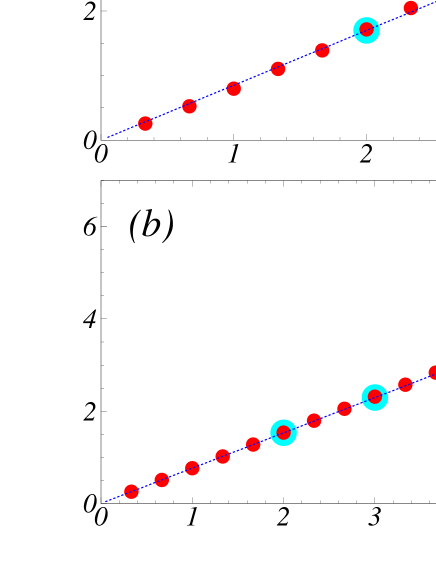
Figure 5: (Colour online) Scaling function $\gamma(q)$ of the moments $\sigma^{(q)}(t)$, given by (44), plotted vs the order $q$. Dotted straight lines have a slope $q\left(1-\frac{{\bar{\alpha}}(0)}{2}\right)$, according to the theoretical prediction (37), extended to real values of $q$. Moments of integer orders are marked by halos. (a) refers to same data of previous figures, for which the scaling exponent ${\bar{\alpha}}(0)=0.3$ is derived in figure 4. The parameters of (b) are: $l_{1}/l_{2}=(\sqrt{5}+1)/2$, $\tan\varphi=\pi/4$ and ${\bar{\alpha}}(0)=0.47$.

6 Numerical simulations and conclusions

From the numerical point of view, we may extend the analysis to moments of the diffusive variable $|\Xi(z,t)|$ of arbitrary positive real order. The $q$-th order moment is

$$\sigma^{(q)}(t)\,=\,\int_{{\mathcal{M}}_{\varphi}}{\rm d}\Omega(z)\left|\Xi(z,t)\right|^{q},\qquad q\in{{\mathbb{R}}}_{+};$$ (44)

the scaling function $\gamma(q)$ is defined by (32), with $\sigma^{(n)}$ replaced by $\sigma^{(q)}$. Note that in spite of having introduced the absolute value respect to the definition (12), we keep the same notation.

Numerical simulations, presented throughout the paper, refer to a billiard table belonging to class 3 with parameters $l_{1}/l_{2}=\pi/2$ and $v_{x}/v_{y}=\tan\varphi=\pi/4$; a second case is shown in figure 5 (b), referring to $l_{1}/l_{2}=(\sqrt{5}+1)/2$.

The analytical expression for the exponent $\gamma(n)$ of the algebraic growth of integer order moments, given by (37), is numerically tested in figure 3, in which the $4$-$th$ order moment is plotted as a function of time $t$ in logarithmic scales. The straight line has a slope $\gamma(4)=3.4$, given by the formula with $n=4$ and ${\bar{\alpha}}(0)=0.3$. Numerical procedure to derive ${\bar{\alpha}}(0)$ is explained below.

Figure 5 displays the scaling function $\gamma(q)$ of absolute moments of arbitrary real order (44), for the two parameters’ pairs $(l_{1}/l_{2},\tan\varphi)$ specified above. Numerically evaluated exponents are shown by dot symbols as a function of $q$; they are calculated by a linear least-square fit of $\ln\sigma^{(q)}(t)$ versus $\ln t$.

Analytical estimates of the exponents of integer order moments are shown by halos, surrounding the dots. Inside the inspected range, numerical data are consistent with a linear dependence of $\gamma(q)$ on $q$. The ratio $\gamma(q)/q$ appears to be constant for fixed parameters $(l_{1}/l_{2},\tan\varphi)$ and to depend only on the spectral index ${\bar{\alpha}}$ in $\theta=0$. This ratio ranges between $1/2$ (normal diffusion) and $1$ (ballistic dispersion). Therefore the square annulus billiard displays a so called “weak” anomalous diffusive (or strong self-similar) process [29, 30].

We finally provide a few further details on the numerical procedures.

The discrete-time directional dynamics at fixed $\varphi$ is evolved up to a time $T=2^{20}$ and the number of initial conditions employed in phase averages ranges from $10^{4}$ to $10^{6}$.

An approximation of the microcanonical measure inside the phase space ${\mathcal{M}}_{\varphi}$ is obtained as follows. The phase average is evaluated by taking a uniform distribution of the particles inside the accessible region of the billiard and the sign of the components of the unity velocity vector $\vec{v}$ is assigned at random. The first collision points with the boundaries of the billiard are taken as initial conditions of the Birkhoff mapping.

Spectral analysis of the signals is reconstructed numerically by employing the Fast Fourier Transform algorithm (FFT), i.e. a finite discrete Fourier Transform for vectors in ${\mathbb{C}}^{2T}$. Two different methods have been tested to calculate the coarse-grained approximation of the (1-dimensional) average density power spectrum (18). According to (15), $m_{\xi}(\theta)$ may be approximated by a direct-FFT of the phase-averaged correlation sequence $C^{ph}_{\xi}(t)$. Alternatively, according (18) and (27), we calculate the square modulus of the direct-FFT of the signal $\xi(B^{t}z)$ of single trajectories and then make a phase average over the initial conditions. Owing to the finite time interval $-T\leq t\leq T$, we multiply time sequences, $C^{ph}_{\xi}(t)$ or $\xi(B^{t}z)$, by a proper windowing function [42]; to reduce the amount of negative values in the former method, we prefer to use a triangular window function $w_{t}=1-|t|/T$, instead of a square windowing function as in the theoretical treatment, because its partial Fourier series is a non negative function. In both methods, the resolution in frequency space is $\Delta\theta=\pi/T$. For the finest resolution, i.e. $T=2^{20}$, the order of magnitude of negative values, in the first method, is $\lesssim 10^{-4}$. Apart from numerical errors, the two methods give the same results, for a fixed resolution. By comparison of the two methods, we get that less than the $1\%$ of the total mass on the torus is affected by numerical errors. In figure 4 (a) a reconstruction of $m_{\xi}(\theta)$ is shown, calculated with a resolution of $\pi/(2^{14})$.

The first two generalized dimensions $D_{1}$ (information dimension) and $D_{2}$ (correlation dimension) [43] are calculated by making a sequence of dyadic partitions of the coarse-grained approximation of $m_{\xi}(\theta)$. At step $N$, the interval $(-\pi,\pi]$ is divided into $2^{N}$ sub-intervals $I_{N,j}$ ($j=1,\cdots,2^{N}$) of length $\delta_{N}=2\pi/2^{N}$, each of which contains a mass $\mu(I_{N,j})$. As $N\to\infty$ (i.e. $\delta_{N}\to 0$), $D_{1}$ and $D_{2}$ are defined by:

$$\chi_{1}(N)={\sum_{j=1}^{2^{N}}\mu(I_{N,j})\ln\mu(I_{N,j})}\sim D_{1}\;{\ln\delta_{N}}$$

$$\chi_{2}(N)={\ln\sum_{j=1}^{2^{N}}\mu^{2}(I_{N,j})}\sim D_{2}\;{\ln\delta_{N}}.$$

We extrapolate $D_{1}$ and $D_{2}$ by a linear fitting in logarithmic scale with $N$ ranging from $N=2$ to $N=20$; an example is shown in figure 2 (b). A value of $D_{1}<1$ is found, consistent with the presence of a singular continuous component of the spectrum. As shown in figure 2 (a), the obtained value of $D_{2}$ gives a satisfactory estimate of the power law decay exponent of the integrated correlation function.

The scaling index ${\bar{\alpha}}$ of the spectral measure in $\theta=0$ is also evaluated numerically. In figure 4 (b) the mass contained in the interval $[-\delta,\delta]$ is shown as a function of $\delta$. Intervals of different widths $\delta_{M}=M\Delta\theta$ are considered, with a resolution $\Delta\theta$ ranging from $\pi/2^{20}$ to $\pi/2^{6}$; different symbols refer to $M=0$ (triangles), $M=1$ (squares) and $M=8$ (circles). The mass is given by $\mu([-\delta_{M},\delta_{M}])=\sum_{j=-M}^{M}m_{\xi}(j\Delta\theta)$ and it is supposed to scales as $\sim\delta_{M}^{{\bar{\alpha}}(0)}$. The straight line, which fits the data in logarithmic scales in the range $-11<ln\delta<-7$, has a slope of ${\bar{\alpha}}(0)=0.30\pm 0.05$. The data in the left part of figure 4 (b) are not taken into account in the derivation of ${\bar{\alpha}}(0)$ because the corresponding mass is close or below the numerical precision of the simulations. The same calculation in case $l_{1}/l_{2}=(\sqrt{5}+1)/2$ gives the value ${\bar{\alpha}}(0)=0.47\pm 0.05$. Note that the error on the numerical estimate of $\bar{\alpha}(0)$ is not relevant when compared with data of figure 5.

We have thus provided analytic arguments and numerical support that polygonal billiards may exhibit anomalous transport in a weak sense [29]: the distribution of the angle, accumulated by single particles at fixed time, is not gaussian and the moments’ asymptotic growth is governed by a single scale, which is related to the Hölder exponent of the spectral measure at zero.

This work has been partially supported by MIUR-PRIN project “Nonlinearity and disorder in classical and quantum transport processes”.

Appendices

Appendix A Power spectrum, bispectrum and trispectrum

For $n=2$, namely for a single frequency $\theta\in{\mathbb{T}}$, the result (27) is retrieved from (23); the weak limit $s_{\xi}(\theta;z)$ of the sequence (27) is the density power spectrum of the signal.

For the first few orders, i.e. $n=3$ and $4$ (bispectrum and trispectrum), we have the following explicit expressions, respectively:

$$M_{T,\xi}(\theta_{1},\theta_{2};{z_{s,l}})=\frac{i}{2T}\rho_{T}(\theta_{1};{z_{s,l}})\rho_{T}(\theta_{2};{z_{s,l}})\rho_{T}(\theta_{1}+\theta_{2};{z_{s,l}})\cdot$$ (45)

$$\qquad\qquad\qquad\qquad\cdot\sin(\phi_{T}(\theta_{1};{z_{s,l}})+\phi_{T}(\theta_{2};{z_{s,l}})-\phi_{T}(\theta_{1}+\theta_{2};{z_{s,l}})),$$

and

$$M_{T,\xi}(\theta_{1},\theta_{2},\theta_{3};{z_{s,l}}) = \frac{1}{2T}\rho_{T}(\theta_{1};{z_{s,l}})\rho_{T}(\theta_{2};{z_{s,l}})\rho_{T}(\theta_{3};{z_{s,l}})\rho_{T}(\theta_{1}+\theta_{2}+\theta_{3};{z_{s,l}})\cdot$$ (46)

$$\quad\cdot\cos(\phi_{T}(\theta_{1};{z_{s,l}})+\phi_{T}(\theta_{2};{z_{s,l}})+\phi_{T}(\theta_{3};{z_{s,l}})-\phi_{T}(\theta_{1}+\theta_{2}+\theta_{3};{z_{s,l}})),$$

with ${z_{s,l}}=(s,\varphi_{l})$ and $\varphi_{l}=\varphi-l\pi/2$ ($l=0,1$).

A.1 Symmetry properties

Owing to the symmetry properties of higher order spectra and of multiple-time phase averaged correlation functions (13), the integration domain in (15) can be reduced. Some properties, as (24), (25) and (26), follow directly from (20) and (8), (9) and have been used to restrict the domain in (5), as explained in section 5.

A general procedure to determine the principal domain of polyspectra, i.e. the nonredundant region of computation, is explained in [38, 39, 44]. The symmetry properties of higher order spectra can be grouped into:

1. invariance under permutation of any pair of frequencies;

2. the conjugate symmetry property (24), which implies the redundancy of half of some frequency axes;

3. periodicity of period $2\pi$ is each frequency variable; this is a consequence of the fact that the partial sums (7) are periodic functions of the frequencies $\theta_{i}\in{\mathbb{T}}$ ($i=1,\cdots,n$).

In this appendix, we review some symmetry conditions for the 2- and 3- dimensional cases [27].

Two dimensional case. From the definition of 2-time phase-averaged correlation function, i.e. (13) with $n=3$, and the invariance of the measure ${\rm d}\Omega(z)$ under $B^{t}_{\varphi}$, we get:

$$C^{ph}(t_{1},t_{2})=C^{ph}(t_{2},t_{1})=C^{ph}(-t_{1},t_{2}-t_{1})=C^{ph}(-t_{2},t_{1}-t_{2}).$$ (47)

From (45), (8) and (9), we have:

$$m(\theta_{1},\theta_{2})=m(\theta_{2},\theta_{1})=m^{*}(-\theta_{1},-\theta_{2})=m(\theta_{1},-\theta_{1}-\theta_{2})=m(\theta_{2},-\theta_{1}-\theta_{2}).$$ (48)

Owing to (48), the bispectrum is symmetric about the lines $\theta_{1}=\theta_{2}$, $\theta_{1}+2\theta_{2}=2\pi n_{1}$ and $\theta_{2}+2\theta_{1}=2\pi n_{2}$ ($n_{1},n_{2}\in{\mathbb{Z}}$). The principal domain is the triangle of vertices $A(0,0)$, $B(\pi,0)$ and $C(\frac{2}{3}\pi,\frac{2}{3}\pi)$, i.e. $0\leq\theta_{1}\leq\frac{2}{3}\pi,\;0\leq\theta_{2}\leq\theta_{1}$ and $\frac{2}{3}\pi\leq\theta_{1}\leq\pi,\;0\leq\theta_{2}\leq-2\theta_{1}+2\pi$.

Three dimensional case. The 3-time phase-averaged correlation function satisfies:

$$C^{ph}(t_{1},t_{2},t_{3})=C^{ph}(t_{1},t_{3},t_{2})=C^{ph}(-t_{1},t_{2}-t_{1},t_{3}-t_{1});$$ (49)

and the trispectrum:

$$m(\theta_{1},\theta_{2},\theta_{3})=m(\theta_{1},\theta_{3},\theta_{2})=m(-\theta_{1},-\theta_{2},-\theta_{3})=m(\theta_{2},\theta_{3},-\theta_{1}-\theta_{2}-\theta_{3}).$$ (50)

Cyclic relations, obtained by permutations of $(t_{1},t_{2},t_{3})$ in (49) and $(\theta_{1},\theta_{2},\theta_{3})$ in (50), hold. The trispectrum is symmetric about the plane $2\theta_{1}+\theta_{2}+\theta_{3}=2\pi n_{1}$ (and cyclic). The principal domain is a polyhedron with vertices $A(0,0,0)$, $B(\frac{\pi}{2},\frac{\pi}{2},\frac{\pi}{2})$, $C(\pi,0,0)$, $D(\frac{2}{3}\pi,\frac{2}{3}\pi,0)$, $E(\pi,0,-\frac{\pi}{2})$ and $F(\pi,\pi,-\pi)$ [39].

Appendix B Dynamical and spectral exponents.

In this appendix we sketch how to derive (30).

We assume that the spectral measure ${\rm d}\mu_{\xi}(\theta)$, associated to $\xi$, is uniformly ${\bar{\alpha}}$-Hölder continuous (U${\bar{\alpha}}$H) in an interval ${\mathcal{I}}_{\Delta}(\tilde{\theta})\equiv[\tilde{\theta}-\Delta,\tilde{\theta}+\Delta]$, namely a positive constant $c$ exists such that

$$\mu_{\xi}({\mathcal{I}}_{\delta}(\theta))\equiv\int_{\theta-\delta}^{\theta+\delta}{\rm d}\mu_{\xi}(\theta^{\prime})\leq c\delta^{{\bar{\alpha}}(\tilde{\theta})},\qquad\;\;\forall{\mathcal{I}}_{\delta}(\theta)\subset{\mathcal{I}}_{\Delta}(\tilde{\theta}).$$ (51)

The sequence $\{m_{T,\xi}(\theta)\}_{T\in{{\mathbb{N}}_{+}}}$ is defined by (18) and (27) as

$$m_{T,\xi}(\theta) = \int_{{\mathcal{M}}_{\varphi}}{\rm d}\Omega(z)s_{T,\xi}(\theta;z)$$

$$= \frac{1}{2T}\int_{{\mathcal{M}}_{\varphi}}{\rm d}\Omega(z)\hat{\xi}_{T}(\theta;z)\hat{\xi}^{*}_{T}(\theta;z).$$

By making use of (7) and then of (3), (15) and (28), we obtain

$$m_{T,\xi}(\theta)=\frac{1}{2T}\sum_{t=-T}^{T-1}\sum_{t^{\prime}=-T}^{T-1}C^{ph}_{\xi}(t-t^{\prime})e^{-i\theta(t-t^{\prime})}=\frac{1}{2\pi}\int_{{\mathbb{T}}}{\rm d}\mu_{\xi}(\theta^{\prime})K_{T}(\theta-\theta^{\prime})$$ (53)

with

$$K_{T}(x) = \frac{1}{2T}\sum_{t_{1}=-T}^{T-1}\sum_{t_{2}=-T}^{T-1}e^{ix(t_{1}-t_{2})}=\frac{1}{2T}\left(d_{T}^{2}(x)-2d_{T}(x)\cos Tx+1\right)=$$ (54)

$$= \frac{1}{2T}\left(\frac{\sin Tx}{\sin\frac{x}{2}}\right)^{2};$$

$K_{T}(x)$ is the Fej$\acute{\rm e}$r kernel, up to a constant factor, and $d_{T}(x)$ is the Dirichlet Kernel:

$$d_{T}(x)=\sum_{t=-T}^{T}e^{ixt}=\frac{\sin\left[(2T+1)\frac{x}{2}\right]}{\sin\frac{x}{2}}.$$ (55)

The kernel (54) is a positive, periodic even function of $x\in{\mathbb{T}}$; moreover, it fulfills:

$$(i) \;K_{T}(0)=2T;$$

$$(ii) \;\lim_{T\to\infty}K_{T}(x)=0\;\;{\rm uniformly}\;\;\;|x|\geq\delta>0;$$

$$(iii) \;0\leq K_{T}(x)\leq 2T\;\;\;\;\;\;|x|\leq\frac{\pi}{T};$$

$$(iv) \;0\leq K_{T}(x)\leq\frac{T}{2k^{2}}\;\;\;\;\;\;k\frac{\pi}{T}\leq|x|\leq(k+1)\frac{\pi}{T}\;\;\;{\rm and}\;\;k\geq 1.$$

$$(v) \;\frac{8T}{\pi^{2}}\leq K_{T}(x)\leq 2T\;\;\;\;\;\;|x|\leq\frac{\pi}{2T}.$$

By using the properties above, the proof of theorem 2.1 in [25] can be reproduced for $m_{T,\xi}(\theta)$. Note that $m_{T,\xi}(\theta)$ corresponds to $G_{T}(\theta)$, and $\beta$ to $1-{\bar{\alpha}}$ in [25].

Let $\theta\in{\mathcal{I}}_{\Delta}(\tilde{\theta})$ and $0<\delta<\pi$, we show that (30) holds in an arbitrary interval ${\mathcal{I}}_{\delta}(\theta)\subset{\mathcal{I}}_{\Delta}(\tilde{\theta})$. ${\mathcal{I}}_{\delta}(\theta)$ can be covered by a finite sequence of intervals: (1) ${\mathcal{I}}^{(0)}\equiv\{\theta^{\prime}\in{\mathbb{T}}/\;|\theta-\theta^{\prime}|\leq\frac{\pi}{T}\}$, in which $(iii)$ holds, and (2) ${\mathcal{I}}^{(k)}\equiv\{\theta^{\prime}\in{\mathbb{T}}/\;k\frac{\pi}{T}\leq\ |\theta-\theta^{\prime}|\leq(k+1)\frac{\pi}{T}\leq\delta\}$, in which $(iv)$ holds.

Moreover, assumption (51) implies that the mass in every interval of length $\pi/T$, included in ${\mathcal{I}}_{\Delta}(\tilde{\theta})$, is bounded by $\mu_{\xi}({\mathcal{I}}_{\frac{\pi}{2T}}(\theta))\leq DT^{-{\bar{\alpha}}(\tilde{\theta})}$, with constant $D>0$ and $T>\bar{T}(\Delta,\theta)$; $\bar{T}$ is chosen so that for $T>\bar{T}$: ${\mathcal{I}}_{\frac{\pi}{2T}}(\theta)\subset{\mathcal{I}}_{\Delta}(\tilde{\theta})$.

Therefore,

$$m_{T,\xi}(\theta)\left|{}_{{\mathcal{I}}_{\delta}(\theta)}\right. = \frac{1}{2\pi}\left\{\int_{{\mathcal{I}}^{(0)}}+\sum_{k}\int_{{\mathcal{I}}^{(k)}}\right\}{\rm d}\mu_{\xi}(\theta^{\prime})K_{T}(\theta-\theta^{\prime})$$ (56)

$$\leq \left(C_{1}+C_{2}\sum_{k=1}^{[\delta T/\pi]}\frac{1}{k^{2}}\right)T^{-{\bar{\alpha}}(\tilde{\theta})}T\leq CT^{1-{\bar{\alpha}}(\tilde{\theta})};$$

$[.]$ denotes the integer part.

Appendix C Upper bound for absolute moments of odd order

As mentioned in section 5, the moments of odd order of the observable $\Xi(z,t)$ vanish due to the symmetry property (25) of $m_{\xi}(\vec{\theta})$; we therefore consider integer moments of the absolute value of the observable $\Xi(z,t)$:

$$\sigma^{(n)}(t)=\int_{{\mathcal{M}}_{\varphi}}{\rm d}\Omega(z)\left|\Xi(z,t)\right|^{n}.$$ (57)

For even $n$ (57) reduces to (12); we are interested to $n$ odd integer ($n>1$).

Since $\left|\Xi(z,t)\right|\leq\sum_{s=0}^{t-1}\left|\xi(B_{\varphi}^{s};z)\right|$, the following bound holds:

$$\sigma^{(n)}(t)\leq\bar{\sigma}^{(n)}(t)=\int_{{\mathcal{M}}_{\varphi}}{\rm d}\Omega(z)\left(\sum_{s=0}^{t-1}\left|\xi(B^{s}z)\right|\right)^{n}.$$ (58)

Therefore, the exponent $\bar{\gamma}(n)$ of the algebraic growth of $\bar{\sigma}^{(n)}(t)$ constitutes an upper bound for the exponent $\gamma(n)$ of (57); $\bar{\gamma}(n)$ is again defined via a discrete Mellin transform (32), with $\sigma$ replaced by $\bar{\sigma}$.

We reproduce calculations in section 4, by starting from the new phase observable $\bar{\xi}(B^{t}z)\equiv\left|\xi(B^{t}z)\right|$. The partial sum of Fourier series, i.e. $\hat{\bar{\xi}}_{T}(\theta;z)=\sum_{t=-T}^{T-1}|\xi(B^{t}z)|e^{-i\theta t}$, verifies the property (cf. (11)):

$$\hat{\bar{\xi}}_{T}(\theta;(s,-\varphi))=+e^{i\theta}\hat{\bar{\xi}}^{*}_{T}(\theta;(s,\varphi)).$$ (59)

By using (59) in the phase average, the following expression for $\bar{M}_{T,\xi}$ is found (cf. (22) and (23)):

$$\bar{M}_{T,\xi}(\vec{\theta};{z_{s,l}})=\frac{1}{2T}\bar{\Gamma}_{T}(\vec{\theta};{z_{s,l}})\bar{\rho}_{T}(\Theta(\vec{\theta});{z_{s,l}})\cos\left(\bar{\Phi}_{T}(\vec{\theta};{z_{s,l}})-\bar{\phi}_{T}(\Theta(\vec{\theta});{z_{s,l}})\right).$$ (60)

$\bar{M}_{T,\xi}$ is now an even function of $\vec{\theta}$ and it shares the same symmetry properties of (23).

For $n=3$, in particular we have:

$$\bar{M}_{T,\xi}(\theta_{1},\theta_{2};{z_{s,l}})=\frac{1}{2T}\bar{\rho}_{T}(\theta_{1};{z_{s,l}})\bar{\rho}_{T}(\theta_{2};{z_{s,l}})\bar{\rho}_{T}(\theta_{1}+\theta_{2};{z_{s,l}})\cdot$$

$$\qquad\qquad\qquad\qquad\cdot\cos(\bar{\phi}_{T}(\theta_{1};{z_{s,l}})+\bar{\phi}_{T}(\theta_{2};{z_{s,l}})-\bar{\phi}_{T}(\theta_{1}+\theta_{2};{z_{s,l}})).$$ (61)

The exponent $\bar{\gamma}(n)$ can be derived by proceeding as in section 5; by denoting $\bar{\bar{\alpha}}(0)$ the Hölder index of ${\rm d}\mu_{|\xi|}$ in 0, we get $\bar{\gamma}(n)=n(1-\bar{\bar{\alpha}}(0)/2)$.

The mass associated to $|\xi|$ in a small interval, centered in 0, is

$$\mu_{|\xi|}({\mathcal{I}}_{\delta}(0))=\lim_{T\to\infty}\frac{\delta}{T}\int_{{\mathcal{M}}_{\varphi}}{\rm d}\Omega(z)\sum_{t=-T}^{T-1}\sum_{t^{\prime}=-T}^{T-1}|\xi(B_{\varphi}^{t}z)\xi(B_{\varphi}^{t^{\prime}}z)|\;{\rm sinc}(\delta(t-t^{\prime})),$$ (62)

with ${\rm sinc}(x)=\sin x/x$. If $\delta\leq\pi/(2T)$, $\mu_{\xi}({\mathcal{I}}_{\delta}(0))\leq\mu_{|\xi|}({\mathcal{I}}_{\delta}(0))$ and therefore $\bar{{\bar{\alpha}}}(0)\leq{\bar{\alpha}}(0)$.

References

References

- [1] Dettmann C P, Cohen E G D and Van Beijeren H 1999 Microscopic chaos from brownian motion? Nature 401 875–6
- [2] Cecconi F, del-Castillo-Negrete D, Falcioni M and Vulpiani A 2003 The origin of diffusion: the case of non-chaotic systems Physica D 180 129–39
- [3] Alonso D, Artuso R, Casati G and Guarneri I 1999 Heat conductivity and dynamical instability Phys.Rev.Lett. 82 1859–62
- [4] Lepri S, Rondoni L and Benettin G 2000 The Gallavotti–Cohen Fluctuation theorem for a nonchaotic model J. Stat. Phys. 99 857–72
- [5] Eckmann J -P and Mejia-Monasterio C 2006 Thermal rectification in billiard-like systems Phys. Rev. Lett. 97 094301–4
- [6] Casati G, Mejia-Monasterio C and Prosen T 2007 Magnetically induced thermal rectification Phys. Rev. Lett. 98 104302–5
- [7] Jepps O G, Bhatia S K and Searles D J 2003 Wall mediated transport in confined spaces: exact theory for low density Phys. Rev. Lett. 91 126102–5
- [8] Friedman N, Kaplan A, Carasso D and Davidson N 2001 Observation of chaotic and regular dynamics in atom-optics billiards Phys. Rev. Lett. 86 1518–21
- [9] Hentschel M and Richter K 2002 Quantum chaos in optical systems: the annular billiard Phys. Rev. E 66 056207–19
- [10] Klages R 2007 Microscopic Chaos, Fractals and Transport in Nonequilibrium Statistical Mechanics Advanced Series in Nonlinear Dynamics vol 24 (World Scientific Co. Pte. Ltd., Singapore)
- [11] Borgonovi F, Casati G and Li B 1996 Diffusion and localization in chaotic billiards Phys. Rev. Lett. 77 4744–7
- [12] Alonso D, Ruiz A and de Vega I 2002 Polygonal billiards and transport: diffusion and heat conduction Phys. Rev. E 66 066131–45
- [13] Li B, Casati G and Wang J 2003 Heat conductivity in linear mixing systems Phys. Rev. E 67 021204–7
- [14] Alonso D, Ruiz A and de Vega I 2004 Transport in polygonal billiards Physica D 187 184–99
- [15] Jepps O G and Rondoni L 2006 Thermodynamics and complexity of simple transport phenomena J. Phys. A: Math. Gen. 39 1311–37
- [16] Sanders D P and Larralde H 2006 Occurrence of normal and anomalous diffusion in polygonal billiard channels Phys. Rev. E 73 026205–13
- [17] Sanders D P 2005 Deterministic diffusion in periodic billiard models PHD Thesis University of Warwick, Coventry, CV4 7AL, U.K.
- [18] Casati G and Prosen T 1999 Mixing property of triangular billiards Phys. Rev. Lett. 83 4729–32
- [19] Artuso R, Casati G and Guarneri I 1997 Numerical study on ergodic properties of triangular billiards Phys. Rev. E 55 6384–90
- [20] Gutkin E 1986 Billiards in polygons Physica D 19 311–33
- [21] Gutkin E 1996 Billiards in polygons: survey of recent results J. Stat. Phys. 83 7–26
- [22] Richens P J and Berry M V 1981 Pseudointegrable system in classical and quantum mechanics Physica D 2 495–512
- [23] Liboff R L and Liu J 2000 The Sinai billiard, square torus, and field chaos Chaos 10 756–9
- [24] Artuso R, Guarneri I and Rebuzzini L 2000 Spectral properties and anomalous transport in a polygonal billiard Chaos 10 189–94
- [25] Hof A 1997 On scaling in relation to singular spectra Comm. Math. Phys. 184 567–77
- [26] Graczyk J and S̀wia̧tek G 1993 Singular measures in circle dynamics Commun. Math. Phys. 157 213–30
- [27] Nikias C L and Mendel J M 1993 Signal processing with higher-order spectra IEEE Signal Processing Magazine 10–37
- [28] Armstead D N, Hunt B R and Ott E 2003 Anomalous diffusion in infinite horizon billiards Phys. Rev. E 67 021110–6
- [29] Castiglione P, Mazzino A, Muratore-Ginanneschi P and Vulpiani A 1999 On strong anomalous diffusion Physica D 134 75–93
- [30] Ferrari F, Manfroi A J and Young W R 2001 Strongly and weakly self-similar diffusion Physica D 154 111–37
- [31] Ketzmerick R, Petschel G and Geisel T 1992 Slow decay of temporal correlations in quantum systems with Cantor spectra Phys. Rev. Lett. 69 695–8
- [32] Holschneider M 1994 Fractal wavelet dimensions and localization Commun. Math. Phys. 160 457–73
- [33] Artuso R and Cristadoro G 2004 Periodic orbit theory of strongly anomalous transport J. Phys. A: Math Gen. 37 85–103
- [34] Schreier P J and Scharf L L 2006 Higher-order spectral analysis of complex signals Signal Processing 86 3321–33
- [35] Mendel J M 1991 Tutorial on higher-order statistics (spectra) in Signal Porcessing and system theory: theoretical results and some applications Proceedings of the IEEE vol 79 n 3 278–305
- [36] Strichartz R S 2003 A guide to distribution theory and Fourier transforms (World Scientific Co. Pte. Ltd., River Edge NJ)
- [37] Abrahamsen P 1997 A review of gaussian random fields and correlation functions Technical report, Tech. Rep. 917 (Norwegian Computing Center)
- [38] Collis W B, White P R and Hammond J K 1998 Higher order spectra: the bispectrum and the trispectrum Mechanical Systems and Signal Processing vol 12(3) 375–94
- [39] Chandran V and Elgar S 1994 A general procedure for the derivation of principal domains of higher-order spectra IEEE Trans, on signal processing vol. 42 n 1 229–33
- [40] Dana I and Dorofeev D L 2006 General quantum resonances of the kicked particle Phys. Rev. E 73 026206–11
- [41] Fan H and Fu L 2003 Normal ordering expansion of n-dimensional radial coordinate operators gained by virtue of the IWOP technique J. Phys. A: Math Gen. 36 1531–6
- [42] Harris F J 1978 On the use of windows for harmonic analysis with the discrete Fourier transform Proc. of IEEE 66 51–83
- [43] Hentschel H G E and Procaccia I 1983 The infinite number of generalized dimensions of fractals and strange attractors Physica D 8 435–44
- [44] Chandran V 1994 On the computation and interpretation of auto- and cross-trispectra Proc. of ICASSP 94 (Adelaide) vol 4 (Australia) 445–8