Understanding Fashion Cycles as a Social Choice

Abstract

We present a formal model for studying fashion trends, in terms of three parameters of fashionable items: (1) their innate utility; (2) individual boredom associated with repeated usage of an item; and (3) social influences associated with the preferences from other people. While there are several works that emphasize the effect of social influence in understanding fashion trends, in this paper we show how boredom plays a strong role in both individual and social choices. We show how boredom can be used to explain the cyclic choices in several scenarios such as an individual who has to pick a restaurant to visit every day, or a society that has to repeatedly ‘vote’ on a single fashion style from a collection. We formally show that a society that votes for a single fashion style can be viewed as a single individual cycling through different choices.

In our model, the utility of an item gets discounted by the amount of boredom that has accumulated over the past; this boredom increases with every use of the item and decays exponentially when not used. We address the problem of optimally choosing items for usage, so as to maximize over-all satisfaction, i.e., composite utility, over a period of time. First we show that the simple greedy heuristic of always choosing the item with the maximum current composite utility can be arbitrarily worse than the optimal. Second, we prove that even with just a single individual, determining the optimal strategy for choosing items is NP-hard. Third, we show that a simple modification to the greedy algorithm that simply doubles the boredom of each item is a provably close approximation to the optimal strategy. Finally, we present an experimental study over real-world data collected from query logs to compare our algorithms.

1 Introduction

When an individual or a society is repeatedly presented with multiple substitutable choices, such as different colors of cars or different themes of musicals, we often observe a recurring shift of preferences over time, or commonly known as fashion trends. While some trends are relatively easy to explain (e.g., sweater sales increasing in the winter), some other trends may result from a variety of factors. In this paper, we first describe a utility model which we think may explain such trends. Then we study the computational issues under the model and provide simple mechanisms by which consumers may make close to optimal decisions on which products to consume and when, in order to maximize their overall utility. We then conduct experiments to show how various parameters in our model can be estimated and to validate our algorithm.

Understanding fashion trends are of significant academic interests as well as commercial importance in various fields, including brand advertising and market economics. Therefore, there’s a large body of work in multiple disciplines – sociology (e.g. [4, 3]), economics (e.g. [7]), and marketing (e.g. [11, 12], on theories for evolution of fashion. Despite much study, there is a lack of a well accepted theory. This is probably not surprising as what makes us like or dislike an alternative and how that changes over time involves economical, psychological, and social factors. Next we describe three such factors that influence fashion.

First, and perhaps the most basic, cause of a product becoming trendy is its utility, intuitively capturing the value it adds to an individual. We call this the innate utility of a product. Second, psychologically, a person’s utility of consuming a product may be discounted by constant consumption of the same item — as one gets tired of existing products, he desires new and different ones. Third, while at an individual level, we have certain inclinations based on our tastes, these are influenced by social phenomena, such as what we see around us, friends’ and celebrities’ preferences.

In this paper, we present a formal model that unifies the aforementioned three broad categories of factors using innate utility, individual boredom, and social influence (as depicted in Figure 1 and explained below). We attempt to construct a mathematical model for these factors and use the model to explain the formation of fashion trends. We use the term item to denote any product, good, concept, or object whose fashion trend we are interested in.

1. Innate utility: The utility of an item captures the innate value the item provides to an individual. We assume it is fixed, independent of other influences.

2. Individual boredom: If we use any item for too long, we get bored of it, and our appreciation for it goes down. This is modeled as a negative component added to the utility. This factor grows if one repeatedly uses the same item and fades away when one stops consuming the item.

3. Social influence: Our valuation of an item can change significantly by the valuation of our friends or influencing people. For example, when we see that many people around us like something we may start liking it; or we may consciously want to differ from some other people around us. We model such influences as a weighted linear combination from other people.

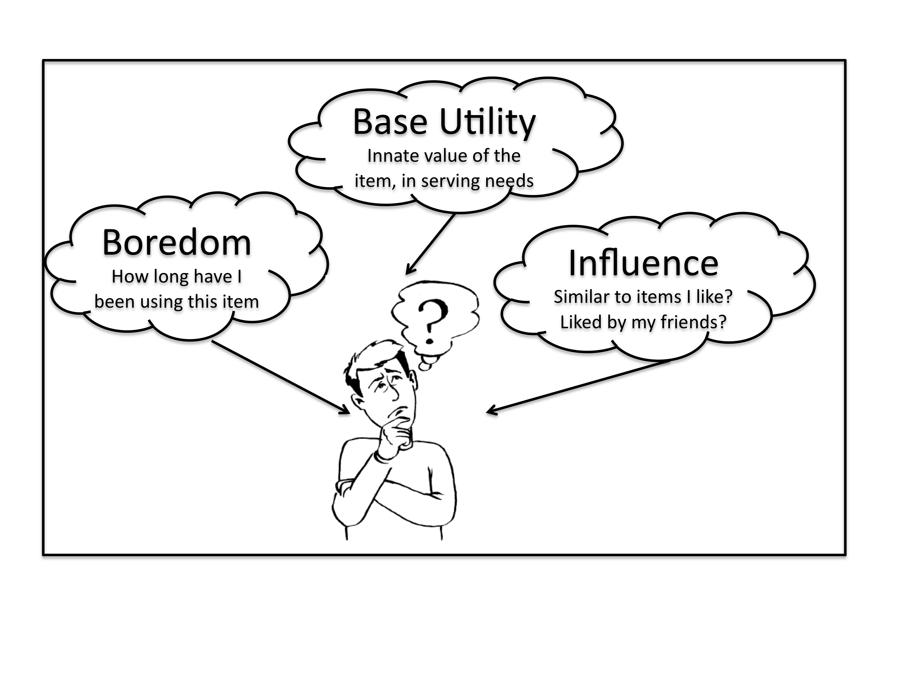
Figure 1: Factors influencing fashion trends

To model boredom on any item at any given time $t$, we associate with each past usage of the item, say at time $t^{\prime}$, a factor in the form of $(1-r)^{t-t^{\prime}}$ for some $r<1$. Then the total boredom on the item takes the sum of the this factor from all the past usage of the item. This definition captures the intuition that the boredom grows if an item is repeatedly used. As we show in our experiments, such exponential decay model matches well people’s interests in songs and movies. The utility maximization under this model, albeit NP-hard, naturally displays cyclic patterns. We also provide a simple strategy to achieve near to optimal utility when the decay factor $r$ is small.

The effect of influence can be formalized using a linear model. For example, to model social influence, consider one item and a society consisting of $m$ people. Let $G$ denote the influence graph on these people that is directed where each edge is labeled with a weight that indicates the strength of this influence. A high value on an edge, such as outgoing edges from celebrities indicates a strong outgoing influence; on the other hand a negative value indicates a desire to distance oneself or be different from the source node. Let $A$ denote the corresponding influence matrix. let $u_{i}(t)$ denote the utility of the item to the $i$th person; let ${\mathbf{u}}(t)$ denote the vector of utilities. If we assume that for each time step the influence from all friends of a person add linearly then we may write ${\mathbf{u}}(t+1)=A{\mathbf{u}}(t)$, which is similar to [11]. Note that for stability of this iterative powers, we should assume that its top eigenvector has magnitude $1$.. We will show that under this influence model, we may treat the society as an individual making choices under the effect of boredom.

Discussion of our results. We argue that fashion trends can be viewed as not just the effect of the influence of a privileged few but more as a democratic process that churns the social boredom and channels the innate instinct for change. Boredom is the innate psychological force that dulls the effect of a constant stimulus over a period of time and make us look for newer stimuli. It is well known that the mind tends to grow oblivious to almost all types of sensations (visual, olfactory, touch, sound) to which it is exposed for a long time. Thus the ‘coolness’ of a fashionable item drops over time and things that we haven’t seen or used in a long time begin to appear more ‘cool’.

We show how several scenarios involving individual and social choices are essentially driven by the same underlying principles. The individual choice may be as simple as choosing a restaurant to visit on a particular day. Alternatively, it may be a social choice where the market forces of a society ‘chooses’ different fashions such as styles for clothing, or cars. Or, a news channel is picking the front page news article to maximize readership and has to choose from different types of news articles, e.g., politics, natural-disaster, celebrity gossip. Each news item may be popular or fashionable for a period of time and then boredom sinks in and the media may switch focus to a different event probably of an entirely different type. Boredom is thus the single most and simplest explanation for oscillations in individual and social choices. This is not at all surprising; indeed boredom is perhaps a strong influence when we make choices such as food, clothes, fashions, governments. Social influence no doubt plays a large part in individual choices. But when we look at the social system as a whole the influences across individuals are forces within the system and in the net effect it simply gives a larger voice to the more influential individuals. We also note that influence by itself is not sufficient to create fashion cycles. In fact, if all influences are positive then without any boredom the system ${\mathbf{u}}(t+1)=A{\mathbf{u}}(t)$ converges to a fixed value resulting in a fixed fashion choice.

Finally, we recognize that the factors we consider are by no means comprehensive; several other ‘external’ factors may change the values of nodes. For example a shortage of oil may increase the utility of green technologies, the strength of the edges in the graph may change, the structure of the graph may change with new node and edge formations. Our decay model for boredom and linear model for influence may be too simplistic. Nonetheless, we believe the influence graph and boredom capture several important aspects of the underlying psychological processes that people use to value items.

Outline of the paper. All the main theoretical results achieved by this paper are presented in Section 2, with proofs appearing in Section 3. Section 4 presents detailed experimental results for validating our model and algorithms; our experiments use real-world data from Google Trends [1] on the popularity of songs and movies in the last 3 years. Related work is presented next and we conclude in Section 5.

Related work. There are several theories of fashion evolution in various communities, e.g., sociologists have modeled fashion trends as a collection of several social forces such as differentiation, influence, and association. While there have been several explanations of cycles in fashion trends [3, 4, 5, 7, 12], most past work does not offer a formal study. We compare our work with one notable exception [11] next. The focus of our paper is on understanding the impact of various factors—boredom, association rules, and utility—on the fashion choices made by individuals and a society. We explain the existence of cycles based on our formal model of fashion, and provide algorithms for making optimal choices.

Reference [11] proposed a formal model of fashion based on association rules. Intuitively, an individual’s utility for an item is impacted by how similar it is to items he likes, and how dissimilar it is to items he dislikes. Further, he is influenced by the society through other individuals’ preferences for various items. Consider a single item, whose consumption vector is given by $c(t)$ at time $t$. Considering the recurrence $c(t+1)=Wc(t)$, where $W$ is the weight influence matrix, [11] observed that if the matrix $W$ has a complex top eigenvalue (corresponding to negative influences), then the item’s consumption pattern may be periodic, producing cycles in preferences. Our model of utility is similar to the consumption model in [11]. However, we consider an additional parameter of boredom that is essential to explain fashion cycles in a society with non-negative influences as such a matrix $W$ always has a real top eigenvalue.

Some other recent work (e.g.,  [6]) study behavioral influences in social networks, such as in terms of information propagation. For instance,  [8] studies how two competing products spread in society, [9] provides techniques for tracking and representing “memes”, which may be used to analyze news cycles, and [10] studies how recommendations propagate in a network through social influence.

The focus of our paper is on formalizing a practical theory for fashion trends with boredom, combined with utility and a simple social behavior. Therefore, for a large part of the paper we consider only a single individual and study fashion trends based on boredom, and utility. Further, in our extension to multiple individuals, we assume a linear weighting of influences from friends’ preferences for particular items.

2 Contributions of Our Study

2.1 Modeling individual boredom

We consider a user living in discrete time periods $0,1,\ldots$ and consuming one item among $n$ substitutable items at each time; for example, a person needs to decide which restaurant to go to every night or which political party to vote for every four years. We assume that each item $i$ brings a base utility $v_{i}$ to the user. Now if we assume that the utilities are fixed then the user would always choose the same item with the maximum $v_{i}$. This would be inconsistent with the observed common behavior of cycling among multiple items, which we refer to as fashion cycles. In order to explain fashion cycles, it is necessary to model the utility dependence of the consumptions across different time periods.

We propose a simple model in which the utility of an item at any time $t$ is the base utility discounted by a boredom factor proportional to the “memory” the person has developed by using this item in the past. The more the user has used the item, the more memory and boredom is developed for the item, and consequently the less utility the item has to the user.

We naturally assume that the memory drops geometrically over time, and the total memory of a person is bounded. This leads to the following definition of memory. Let $0<r<1$ be a memory decay rate, i.e., the rate at which a person “forgets” about things. Let $x_{i}(t)\in\{0,1\}$ indicate if the user uses the item $i$ at time $t$. Then the memory of $i$ at time $t$ is $M_{i}(t)=r\sum_{\tau=0}^{t-1}x_{i}(\tau)(1-r)^{t-\tau}$. We add the factor $r$ so that $M_{i}(t)\leq 1$. The boredom $b_{i}(t)=\alpha_{i}M_{i}(t)$ is proportional to the memory and depends on the item. The utility of item $i$ is defined as $u_{i}(t)=v_{i}-b_{i}(t)=v_{i}-\alpha_{i}M_{i}(t)$. Henceforth, we will refer to $v$ as the base utility and $\alpha$ as the boredom coefficient.

2.2 Utility optimization with boredom

With the above model, one natural question is to compute the choices of the items to maximize the user’s overall utility. If we allow the user to choose at continuous time, the maximization problem becomes relatively easy as the best way to consume an item is to do it cyclically at regular time intervals. However, such regular placement may not be realizable or is hard to find. As we will show below, it is NP-hard to compute the best consumption sequence.

We also consider the natural greedy strategy and show that the under the greedy strategy, the utility of each item is always bounded in a narrow band and so each item is consumed approximately cyclically. The greedy strategy, however, may have produce a sequence giving poor overall utility. We provide a simple heuristics, called double-greedy strategy, and show that it emulates the cyclic pattern of the optimal solution on the real line and yields utility close to the optimal when $r$ is small.

2.2.1 Greedy algorithm

In the greedy strategy, at each time $t$, the user consumes the item with the maximum utility $u_{i}(t)$. This strategy is intuitive and probably consistent with how we make our daily decisions. We show that the utility gap between any two items is small all the time. We provide an example to show it has poor performance in terms of utility maximization. Denote by $\alpha=\max_{i}\alpha_{i}$.

Theorem 2.1.

There exists a time $T$ such that for any $t\geq T$, $u\leq\max_{i}u_{i}(t)\leq u+O(r\alpha\log n)$ where $u$ is the unique solution to the following system:

For all items with $f_{i}>0$, the quantity $v_{i}-f_{i}\alpha_{i}=\mu$; if $f_{i}=0$ then $v_{i}<\mu$; and $\sum f_{i}=1$.

While the greedy algorithm has the nice property of keeping the utility gap between any items small, it may produce a sequence with poor overall utility.

Observation 2.1.

The Greedy strategy of always picking the highest utility item each day is not optimal.

To see the non-optimality of greedy, simply consider two items for beverage, say “water” and “soda”. Assume water has low base utility say $1$ that never changes and zero boredom coefficient. Soda on the other hand has high utility say $10$ but also a high boredom coefficent say $10$. So if one drank soda every day its utility would drop to below that of water. Observe that the greedy strategy will choose soda till its utility drops to that of water and then it is chosen whenever its utility rises even slightly over $1$. So the average utility of the greedy strategy is close to $1$. A smarter strategy is to hold off on the soda even if it is a better choice today so as to enjoy it even more on a later day. Thus it is possible to derive an average utility that is much higher than $1$. For example, we can get average utility of about $3$ by alternating between water and soda in the above example. Note that the greedy algorithm produces poor performance in the above example even for small $r$.

This naturally raises the question: what is the optimal strategy? More importantly is there an optimal strategy that is a simple ’rule of thumb’ that is easy to remember and employ as we make the daily choices. Unfortunately it turns out that computing the optimal strategy is NP-hard.

2.2.2 NP-hardness

Theorem 2.2.

Given a period $T$, target utility $U^{\ast}$, and $n$ items, it is NP-hard to determine whether there exists a selection of items with period $T$ such that the total utility of the selection is at least $U^{\ast}$.

2.2.3 Double-greedy algorithm

On the positive side we show that there is indeed a simple “rule of thumb” that gives an almost optimal solution when $r$ is small. The strategy “double-greedy” waits longer for items that we get bored of too quickly. It is a simple twist on the greedy strategy: instead of picking the item that maximizes the utility $u_{i}(t)=u_{i}-b_{i}(t)$, it picks the one which maximizes $w_{i}(t)=u_{i}-2b_{i}(t)$. Thus it doubles the boredom of all items and then runs the greedy strategy. We show that:

Theorem 2.3.

Let $\overline{U}$ denote the average utility obtained by the double greedy algorithm and $U^{\ast}$ the optimal utility. Then $\overline{U}\geq U^{\ast}-O(r\alpha\log n)$ where $\alpha=\max_{i}\alpha_{i}$.

We note that when $r\to 0$, the utility produced by double greedy is close to the optimal solution.

2.3 Fashion as a Social Choice

A choice is a fashion, if it is the choice of a large fraction of the society. Thus a society only supports a small number of fashions. Industries often target one type of fashion for each market segment. Consider a situation where the entire society consists of one fashion market segment. We will see how in this case such a society can be compared to an individual making choices to maximize utility under the effect of boredom. Each individuals utiltities depend not only on his base utility and boredom but also on the influence from other individuals.

Consider a society of $n$ people and $m$ possible item choices. The society needs to choose one item out of these at every time step. We will study the problem of the makiing the optimal choice so as to maximize welfare. This is applicable in the following scenarios: A business is launching the next fashion style for its market segment, or a radio channel is broadcasting songs in a sequence to maximize the welfare to its audience. Let $u_{ij}(t+1)$ denote the utility of item $i$ to person $j$ at time $t$; let $b_{ij}(t)$ denote the boredom value; let ${\mathbf{u}}_{i}(t)$ denote the vector of utitilities to the $n$ people for item $i$, ${\mathbf{v}}_{i}(t)$ denote the vector of base utilities, and ${\mathbf{b}}_{i}(t)$ denote the vector of boredom values. In the absence of boredom we will say ${\mathbf{u}}_{i}(t+1)=A{\mathbf{u}}_{i}(t)$ where $A$ is the influence matrix. Accounting for boredom we will say, ${\mathbf{u}}_{i}(t+1)=A\ u_{i}(t)-[{\mathbf{b}}_{i}(t+1)-{\mathbf{b}}_{i}(t)]$. Note that this is consistent with the case when there is only one individual where $u_{i}(t+1)=u_{i}(t)-[b(t+1)-b(t)]$. Observe that ignoring the effect of boredom we simply get the recurrence ${\mathbf{u}}_{i}(t+1)=A{\mathbf{u}}_{i}(t)$ or ${\mathbf{u}}_{i}(t)=A^{t}{\mathbf{v}}_{i}$. This recurrence reflects the diffusion of influence through the social network. Note that if the largest eigenvalue of $A$ has magnitude more than $1$ then the process will diverge and if all eigenvalues are $<1$ it will eventually converge to $0$. So we will assume the maximum eigenvalue of $A$ is has magnitude $1$. If the gap between the magnitude of the largest and the second largest eigenvalue is at least ${\epsilon}$ then this diffusion process converges quickly in about $\tilde{\Theta}(1/{\epsilon})$ steps. We will focus on the case when rate of boredom $r$ is much slower than the diffusion rate (this corresponds to the case where influences spread fast and the boredom grows slowly). We then study the problem of making social choices of items over time so as to maximize welfare.

We will assume that $A$ is diagonlizable and has a real top eigenvalue of $1$ and all the other eigenvalues are smaller in magnitude. In that case it is well known that for any vector $x$  $A^{t}x$ converges to to a fixed point and the speed of convergence depends on the gap between the largest and second largest eigenvalue. We show that under certain conditions if $r/\epsilon$ is small then. the choices made by the society is comparable to the choices made by an individual with appropriate base utilities and boredom coefficients. Let $W_{i}(t)$ denote the welfare of the society at time $t$ by choosing item $i$; then $W_{i}(t)/n$

Theorem 2.4.

Consider a society with influence matrix $A$ that has largest eigenvalue $1$ and second largest eigenvalue of magnitude at most $1-{\epsilon}$. For computing the welfare over a a sequence of social choices approximately, such a society can be modelled as a single individual with base uitilities $\tilde{v}_{i}$ and boredom coefficients $\tilde{\alpha}_{i}$, where $\tilde{v}_{i}={\mathbf{c}}^{\prime}{\mathbf{v}}_{i}$ and $\tilde{\alpha}_{i}={\mathbf{c}}^{\prime}{\mathbf{\alpha}}_{i}$ for some vector ${\mathbf{c}}$. Let $\tilde{u}_{i}(t)$ denote the utility of item $i$ to such an individual at time $t$.

More precisely, differences in the average utility of the society for the same sequence of choices until any time $|W_{i}(t)/n-\tilde{u}_{i}(t)|\leq\frac{r}{{\epsilon}}O(|{\mathbf{\alpha}}_{i}|_{\infty})$ for any $t>T$ for some fixed $T$. The $O$ notation hides factors that depends on $A$. For a real, symmetric matrix the constant is $1$

3 Technical details

3.1 Individual choice

The following Lemma is used in the proof of Theorem 2.1.

Lemma 3.1.

$\sum_{i}M_{i}(t)\leq 1$, and $\sum_{i}M_{i}(t)\to 1$ for large $t$. When $t=\Omega(1/r)$, $\sum_{i}M_{i}(t)=1-O(\exp(-tr))$.

Proof.

Observe that the memory scales down by a factor of $1-r$ each time step; exactly one item is picked and $r$ is added to its memory. So $\sum_{i}M_{i}(t+1)=(1-r)\sum_{i}M_{i}(t)+r$. This recurrence gives, $\sum_{i}M_{i}(t)=(1-r)^{t}\sum_{i}M_{i}(0)+r\sum_{j=0}^{t}(1-r)^{j}+(1-r)^{t}(\sum_{i}M_{i}(0)-1)$. Since $M_{i}(0)=0$, $\sum_{i}M_{i}(t)\leq 1$. Observe also that after t = $\Omega(1/r)$ steps this becomes $1+O(exp(-tr))$ ∎

We are now ready to prove Theorem 2.1.

Proof.

(Theorem 2.1) To see that the solution to the given system is unique, note that $f_{i}=(\frac{v_{i}-u}{\alpha})^{+}$ (where $x^{+}$ denotes $max(x,0)$, and so $\sum_{i}(\frac{v_{i}-u}{\alpha})^{+}=1$. This must have a unique solution as $\sum_{i}(\frac{v_{i}-u}{\alpha})^{+}$ is decreasing function of $u$ and strictly decreasing as long as the sum is positive. Let $u$ denote the solution to the above system.

We now show $\max_{i}u_{i}(t)\geq u$ for any $t$. This is done by contradiction. Suppose that for all $i$ $u_{i}(t)<u$. We have that $\sum_{i}(\frac{v_{i}-u}{\alpha_{i}})^{+}<\sum_{i}\frac{v_{i}-u_{i}(t)}{\alpha_{i}}$. But $\sum_{i}\frac{v_{i}-u_{i}(t)}{\alpha_{i}}=\sum_{i}M_{i}(t)\leq 1$. We have that $\sum_{i}(\frac{v_{i}-u}{\alpha_{i}})^{+}<1$, a contradiction.

Let $S_{g}$ denote the set of all the items ever picked by the greedy algorithm. Let $T$ be the time by which each item in $S_{g}$ has been used at least once. By Lemma 3.1, after some steps $\sum_{i}M_{i}(t)$ converges to arbitrarily close to $1$. Lets assume for simplicity of argument that it is exactly $1$ with sufficiently large $T$. To show the upper-bound on $\max_{i}u_{i}(t)$, we show that for $t\geq T$ and any $i\in S_{g}$, $\max_{j}u_{j}(t)-u_{i}(t)=O(\alpha r\log n)$.

Denote by $x(t)$ the item that has the maximum utility at time $t$. It suffices to show that $u_{x(t)}(t)\leq u_{i}(t)+O(\alpha r\log n)$. We recursively compute a decreasing sequence of $t_{j}$ as follows. Let $t_{1}=t$. For $j>1$, suppose we have computed $t_{j-1}$. Let $S_{j-1}=\{x(t_{1}),x(t_{2}),\cdots,x(t_{j-1})\}$. Now let $t_{j}=\max_{t^{\prime}<t_{j-1},x(t^{\prime})\notin S_{j-1}}t^{\prime}$. We stop when there is $k$ such that $x(t_{k})=i$. Since $t>T$, the process is guaranteed to stop. By the above construction, we know only items in $S_{j-1}$ are picked by the greedy algorithm in the interval $[t_{j}+1,t_{1}]$. For any $S\subseteq\{1,\cdots,n\}$, let $A(S,t)=\sum_{\ell\in S}\frac{u_{\ell}(t)}{\alpha_{\ell}}$, and $B(S)=\sum_{\ell\in S}\frac{1}{\alpha_{\ell}}$. We will show that for $1<j\leq k$.

$$A(S_{j-1},t_{j-1})\leq\frac{B(S_{j-1})}{B(S_{j})}A(S_{j},t_{j})+r\,.$$ (1)

First observe that

$$A(S,t)=\sum_{\ell\in S}\frac{u_{\ell}(t)}{\alpha_{\ell}}=\sum_{\ell\in S}\frac{V_{\ell}-\alpha_{\ell}M_{\ell}(t)}{\alpha_{\ell}}=\sum_{\ell\in S}\frac{V_{\ell}}{\alpha_{\ell}}-\sum_{\ell\in S}M_{\ell}(t)\,.$$ (2)

(1) follows from the following claims.

Claim 1.

$A(S_{j-1},t_{j-1})\leq A(S_{j-1},t_{j}+1)$.

Proof.

Since any item picked by the greedy algorithm in $[t_{j}+1,t_{j-1}]$ is in $S_{j-1}$, we have that for $t^{\prime}\in[t_{j}+1,t_{j-1})$, $\sum_{\ell\in S_{j-1}}M_{\ell}(t^{\prime}+1)=(1-r)\sum_{\ell\in S_{j-1}}M_{\ell}(t^{\prime})+r\geq\sum_{\ell\in S_{j-1}}M_{\ell}(t^{\prime})$. The last inequality is by $\sum_{\ell}M_{\ell}(t^{\prime})\leq 1$. Therefore $\sum_{\ell\in S_{j-1}}M_{\ell}(t_{j-1})\geq\sum_{\ell\in S_{j-1}}M_{\ell}(t_{j}+1)$. By (2), we have $A(S_{j-1},t_{j-1})\leq A(S_{j-1},t_{j}+1)$. ∎

Claim 2.

$A(S_{j-1},t_{j}+1)\leq A(S_{j},t_{j})+r$.

Proof.

Since $t_{j}\notin S_{j-1}$ is the item picked by the greedy algorithm at $t_{j}$, $\sum_{\ell\in S_{j-1}}M_{\ell}(t_{j}+1)=(1-r)\sum_{\ell\in S_{j-1}}M_{\ell}(t_{j})$. Thus $\sum_{\ell\in S_{j-1}}M_{\ell}(t_{j}+1)-\sum_{\ell\in S_{j-1}}M_{\ell}(t_{j})=r\sum_{\ell\in S_{j-1}}M_{\ell}(t_{j})\leq r$. Again by (2), we have $A(S_{j-1},t_{j}+1)\leq A(S_{j},t_{j})+r$. ∎

Claim 3.

$A(S_{j-1},t_{j})\leq\frac{B(S_{j-1})}{B(S_{j})}A(S_{j},t_{j})$.

Proof.

Immediately follows from $u_{t_{j}}(t_{j})\geq u_{\ell}(t_{j})$ for $\ell\in S_{j-1}$. ∎

Repeating (1), we have that

$$A(S_{j-1},t_{j-1})$$

$$\leq \frac{B(S_{j-1})}{B(S_{j})}A(S_{j},t_{j})+r\leq\frac{B(S_{j-1})}{B(S_{j})}\left(\frac{B(S_{j})}{B(S_{j+1})}A(S_{j+1},t_{j+1})+r\right)+r$$

$$= \frac{B(S_{j-1})}{B(S_{j+1})}A(S_{j+1},t_{j+1})+r\cdot\frac{B(S_{j-1})}{B(S_{j})}+r\cdots\leq\frac{B(S_{j-1})}{B(S_{k})}A(S_{k},t_{k})+r\cdot\sum_{\ell={j-1}}^{k-1}\frac{B(S_{j-1})}{B(S_{\ell})}\,.$$

Hence, we have that

$$u_{x(t_{1})}(t_{1})=\alpha_{1}A(S_{1},t_{1})\leq\alpha_{1}\left(\frac{B(S_{1})}{B(S_{k})}A(S_{k},t_{k})+r\cdot\sum_{\ell=1}^{k-1}\frac{B(S_{1})}{B(S_{\ell})}\right)=\frac{1}{B(S_{k})}A(S_{k},t_{k})+r\cdot\sum_{\ell=1}^{k-1}\frac{1}{B(S_{\ell})}\,.$$

Since $i=x(t_{k})$, for any $i^{\prime}$, $u_{i^{\prime}}(t_{k})\leq u_{i}(t_{k})$. Therefore $A(S_{k},t_{k})=\sum_{j\in S_{k}}\frac{u_{j}(t_{k})}{\alpha_{j}}\leq u_{i}(t_{k})\sum_{j\in S_{k}}\frac{1}{\alpha_{j}}=u_{i}(t_{k})B(S_{k})$. By that $\alpha=\max_{i}\alpha_{i}$, we have $B(S_{\ell})\geq\ell/\alpha$. Hence

$$u_{x(t_{1})}(t_{1})\leq\frac{1}{B(S_{k})}A(S_{k},t_{k})+r\cdot\sum_{\ell=1}^{k-1}\frac{1}{B(S_{\ell})}\leq u_{i}(t_{k})+\alpha r\sum_{\ell=1}^{k-1}1/\ell=u_{i}(t_{k})+O(\alpha r\log n)\,.$$

Since item $i$ is not used during the interval of $[t_{k}+1,t_{1}]$, we have $u_{i}(t_{k}+1)\leq u_{i}(t_{1})$, and hence $u_{i}(t_{k})\leq u_{i}(t_{k}+1)+\alpha_{i}r\leq u_{i}(t_{1})+\alpha_{i}r$. Therefore we have that, $\max_{j}u_{j}(t_{1})=u_{x(1)}(t_{1})\leq u_{i}(t_{1})+O(\alpha r\log n)$.

On the other hand, we know that there exists $i\in S_{g}$ such that $u_{i}(t)\leq u$ because otherwise it would be the case that $\sum_{i}(\frac{v_{i}-u}{\alpha_{i}})^{+}>\sum_{i}\frac{v_{i}-u_{i}(t)}{\alpha_{i}}=\sum_{i}M_{i}(t)\approx 1$, a contradiction. Hence $\max_{j}u_{j}(t)=u+O(\alpha r\log n)$. ∎

3.2 NP-hardness of item selection

A selection $Y$ is periodic with period $T$, if for any $t$, $y(t+T)=y(t)$, where $y(t)$ is the item chosen at time $t$. Clearly, in a periodic selection, the utility of the item chosen at time $t$ is the same as the one chosen at time $t+T$. For utility maximization, it suffices to consider those items chosen in $[0,T)$. Let $U(Y)=\sum_{t=0}^{T-1}u_{y(t)}(t)$ denote the total utility of $Y$ in $[0,T)$.

Theorem 3.2.

It is NP-hard to decide, given $T$, and $U^{\ast}$, and $n$ items, whether there exist a assignment $Y$ with period $T$ such that $U(Y)\geq U^{\ast}$.

Proof.

The reduction is from the Regular Assignment Problem and is detailed in the appendix. ∎

3.3 Optimality of double-greedy algorithm

Using the exactly same argument in the proofs of Theorem 2.1, we have that

Lemma 3.3.

There exists a time $T$ such that for any $t\geq T$, $\mu\leq\max_{i}w_{i}(t)\leq\mu+O(\alpha\log nr)$ where $\mu$ is the unique solution to the following system:

For all items with $f_{i}>0$, the quantity $v_{i}-2f_{i}\alpha_{i}=\mu$; if $f_{i}=0$ then $v_{i}<\mu$; and $\sum f_{i}=1$.

By using the above theorem, we can prove Theorem 2.3 as follows.

Proof.

(Theorem 2.3) For $0<f\leq 1$, write $\Delta(f)=r\cdot\frac{(1-r)^{1/f}}{1-(1-r)^{1/f}}$.

Let $U^{\ast}$ be the optimal value of the following program.

$$\max U=\sum_{i}f_{i}(v_{i}-\alpha_{i}f_{i})\quad\mbox{s.t.}\quad\sum_{i}f_{i}\leq 1\quad\mbox{and $f_{i}\geq 0$.}$$ (3)

Let $OPT$ denote the optimal average utility. We have that $OPT\leq U^{\ast}+\alpha r$. This is by observing that for any $0<f<1$, placing an item $1/f$ apart gives an upper bound on the utility of consuming the item with frequence $f$. The bound is $v-\alpha\Delta(f)\leq v-\alpha(r-f)$ by observing that $\Delta(f)>r-f$.

The objective of (3) is maximized when there exists $\lambda$ such that $\frac{\partial U}{\partial f_{i}}=\lambda$ for $f_{i}>0$ and $\frac{\partial U}{\partial f_{i}}<\lambda$ for $f_{i}=0$, and $\sum_{i}f_{i}=1$. Since $\frac{\partial U}{\partial f_{i}}=v_{i}-2\alpha_{i}f_{i}$, $\lambda$ is exactly the same as $\mu$ in the statement of Lemma 3.3. This explains the intuition of the double greedy heuristics — it tries to equalize the marginal utility gain of each item. Denote the optimal solution by $f_{i}^{\ast}$. Then for $f_{i}^{\ast}>0$, $v_{i}-2\alpha_{i}f_{i}^{\ast}=\mu$. Hence,

$$U^{\ast}=\sum_{i}f_{i}^{\ast}(v_{i}-\alpha_{i}f_{i}^{\ast})=\sum_{i}f_{i}^{\ast}(\mu+\alpha_{i}f_{i}^{\ast})=\mu+\sum_{i}\alpha_{i}{f_{i}^{\ast}}^{2}\,.$$

Let $k_{i}$ denote the number of times item $i$ is used in $[0,T]$ by the double-greedy algorithm, and $f_{i}=k_{i}/T$. Let $\overline{M}_{i}$ denote the average memory on $i$ at the times when $i$ is picked. Then we have that

$$\overline{U} = \sum_{t=0}^{T}u_{x(t)}(t)/T=\sum_{i}\sum_{x(t)=i}u_{i}(t)/T=\sum_{i}\sum_{x(t)=i}(w_{i}(t)+\alpha_{i}M_{i}(t))/T$$ (4)

$$\geq \sum_{i}\sum_{x(t)=i}(\mu+\alpha_{i}M_{i}(t))/T\quad\mbox{(by Lemma~{}\ref{lem:gap2}, $w_{i}(t)\geq\mu$)}$$

$$\geq \mu+\sum_{i}\alpha_{i}f_{i}\overline{M}_{i}\,.$$

Write $\delta=\alpha r\log n$. By Lemma 3.3, $w_{i}(t)=\mu+O(\delta)$ for each $i,t$. We will show that

Claim 1. $\alpha_{i}f_{i}=\alpha_{i}f_{i}^{\ast}-O(\delta)$.

Observe that for any item $i$ which is picked $k_{i}$ times in $[0,T]$, $\min_{0\leq t\leq T}M_{i}(t)\leq\Delta(k_{i}/T)\leq k_{i}/T=f_{i}$. Hence, $\max_{t}w_{i}(t)\geq v_{i}-2\alpha_{i}M_{i}(t)\geq v_{i}-2\alpha_{i}f_{i}$. On the other hand, $w_{i}(t)=\mu+O(\delta)$. We have $v_{i}-2\alpha_{i}f_{i}=\mu+O(\delta)$. But $\mu=v_{i}-2\alpha_{i}f_{i}^{\ast}$. Therefore $\alpha_{i}f_{i}\geq\alpha_{i}f_{i}^{\ast}-O(\delta)$.

Claim 2. $\alpha_{i}\overline{M}_{i}=\alpha_{i}f_{i}^{\ast}-O(\delta)$.

Since $v_{i}-2\overline{M}_{i}\leq\mu+\delta$, we obtain the bound by following the same argument as in the proof of Claim 1. Now, plugging both claims into (4), we have that

$$\overline{U}\geq\mu+\sum_{i}\alpha_{i}(f_{i}^{\ast}-\frac{O(\delta)}{\alpha_{i}})^{2}\geq\mu+\sum_{i}\alpha_{i}{f_{i}^{\ast}}^{2}-O(\delta)=U^{\ast}-O(\delta)=OPT-O(\delta)\,.$$

This last equality follows from $U^{\ast}=OPT-\alpha r$. This completes the proof. ∎

3.4 Social Choice is equivalent to individual choice

Let ${\bf 1}$ denote the vector with all coordinates set to $1$ and ${\mathbf{\alpha}}_{i}$ denote the vector of boredom coefficients $\alpha_{ij}$.

Observation.

For any diagonolizable matrix $A$ with largest eigenvalue $1$ and the second largest eigenvalue is at most $1-{\epsilon}$, there is a vector $c$ so that. ${\bf 1}^{\prime}A^{t}x-c^{\prime}x\leq(1-{\epsilon})^{t}\sqrt{n}O(|x|_{2})$. The $O$ notation hides factors that depends on $A$. For a real, symmetric matrix the constant is $1$.

Proof.

We will sketch the proof for real symmetric matrices. The same idea holds for non-symmetric matrices. If $p_{1},\ldots,p_{n}$ denote the eigenvectors of $A$ and $1=\lambda_{1},\ldots,\lambda_{n}$ denote the eigenvalues then $A^{t}x=\sum_{j}\lambda^{t}_{j}p_{i}v^{\prime}_{i}x=p_{1}v^{\prime}_{1}x+\sum_{j>1}{\lambda^{t}}_{j}p^{\prime}_{i}p_{i}x$. Now,—$\sum_{j>1}\lambda^{t}_{j}p^{\prime}_{i}p_{i}x|_{2}\leq(1-{\epsilon})^{t}|x|_{2}$. So $|{\bf 1}^{\prime}(A^{t}x-p_{1}p^{\prime}_{1}x)|\leq|{\bf 1}|_{2}(1-{\epsilon})^{t}|x|_{2}=\sqrt{n}(1-{\epsilon})^{t}|x|_{2}$ Setting $c={\bf 1}^{\prime}v_{1}v^{\prime}_{1}$ completes the proof. ∎

We will now prove theorem 2.4

Proof.

(Theorem 2.4) Let $\Delta{\mathbf{b}}(t)$ denote ${\mathbf{b}}(t)-{\mathbf{b}}(t-1)$. Now ${\mathbf{u}}_{i}(t)=A{\mathbf{u}}_{i}(t-1)+\Delta{\mathbf{b}}(t)$. This gives, ${\mathbf{u}}_{i}(t)=A^{t}{\mathbf{v}}_{i}+\sum_{j=0}^{t-1}A^{j}\Delta{\mathbf{b}}(t)$. Note that $W_{i}(t)$ = ${\bf 1}^{\prime}{\mathbf{u}}_{i}(t)={\bf 1}^{\prime}A^{t}{\mathbf{v}}+\sum_{j=0}^{t-1}{\bf 1}^{\prime}A^{j}\Delta\ b(t-j)$

Note $\Delta b_{ij}(t)=\alpha_{ij}((1-r)M_{ij}(t)+rI_{i}(t)-M_{ij}(t))=\alpha_{ij}r(x_{i}(t)-M_{ij}(t))$. So $|\Delta b_{ij}(t)|_{2}\leq r|{\mathbf{\alpha}}_{i}|_{2}$.

Now $|{\bf 1}^{\prime}A^{t}{\mathbf{v}}_{i}-c^{\prime}{\mathbf{v}}_{i}|\leq(1-{\epsilon})^{t}\sqrt{n}O(|{\mathbf{v}}_{i}|_{2})$. For $t>(1/{\epsilon})\Omega(\log(nr|{\mathbf{v}}_{i}|_{2})$, this is at most $r$. Also $|{\bf 1}A^{j}\Delta{\mathbf{b}}_{i}(t-j)-c^{\prime}\Delta{\mathbf{b}}_{i}(t-j)|\leq(1-{\epsilon})^{j}\sqrt{n}O(|\Delta{\mathbf{b}}_{i}(t-j)|_{2})\leq(1-{\epsilon})^{j}\sqrt{n}rO(|{\mathbf{\alpha}}_{i}|_{2})$. So, $|\sum_{j}{\bf 1}A^{j}\Delta{\mathbf{b}}_{i}(t-j)-\sum_{j}c^{\prime}\Delta{\mathbf{b}}_{i}(t-j)|\leq(r/{\epsilon})\sqrt{n}O(|{\mathbf{\alpha}}_{i}|_{2})$. So, $|\sum_{j}{\bf 1}A^{j}\Delta{\mathbf{b}}_{i}(t-j)-c^{\prime}\ b_{i}(t)|\leq(r/{\epsilon})\sqrt{n}O(|{\mathbf{\alpha}}_{i}|_{2})$. Therefore $|W_{i}(t)-(c^{\prime}{\mathbf{v}}_{i}-c^{\prime}{\mathbf{b}}_{i}(t))|\leq(r/{\epsilon})O(\sqrt{n}|{\mathbf{\alpha}}_{i}|_{2})$. Dividing by $n$ completes the proof. ∎

4 Experiments

In this section, we provide experimental results to study the techniques presented in the paper. Our primary objectives is to evaluate the quality of greedy and double-greedy algorithms for choosing items based on utility and boredom parameters estimated from the real data.

4.1 Setup

We obtain data on the popularity of songs and movies from Google Trends [1]. We collected weekly aggregate counts from query logs for popular songs from the last 3 years. Similar data was collected for popular movies. While the popularity of songs and movies depends on additional factors such as awards won by an album or a movie, our goal was to perform a controlled experiment only based on overall utility and boredom. Therefore, for each item we collected weekly aggregate counts starting from the highest peak in logs till there was an “artificial peak” due to an external event such as an award. Further, we compare the utility obtained by our model with a baseline in which the user selects an item simply based on its utility without any discounting from boredom. We describe how we compute the values of $\alpha$, $v$, and $r$ in the appendix.

Song $v$ $\alpha$ $r$ The Climb 12.3 9.9 0.097 Lucky 2.6 1.58 0.114 Snow Patrol - Chasing Cars 10.7 6.8 0.127 I know you want me 7.95 6.5 0.077 Viva la vida 12.4 9.1 0.16 Stop and stare 10.5 9.4 0.092 Disturbia 8 7.2 0.092 Pocket full of sunshine 7.6 6.3 0.14 Supernatural superserious 24.2 22 0.15 One step at a time 9.35 8.5 0.075 Table 1: $v,\alpha,r$ for the set of songs.

Movie $v$ $\alpha$ $r$ Godfather 6.15 5.15 0.123 Hancock 9.6 8.8 0.128 The Bucket List 13.1 11.8 0.102 Quantum of Solace 29.8 29 0.111 Tropic Thunder 25.6 24.8 0.082 Table 2: $v,\alpha,r$ for the set of movies.

Table 2 shows the $v$, $\alpha$, and $r$ values for a set of 10 songs used in our experiments while the corresponding data for the movie data set is shown in Table 2; here we allow different values of $r$, but we notice that all $r$-values within the domain of songs and movies are similar.

4.2 Results

We ran a set of experiments to verify the effectiveness of the greedy and double-greedy heuristics. We ran the experiments over $100000$ steps for both the data sets. The average utility obtained by the user for both the data sets was computed and is shown in Table 3. We also show results for the baseline approach that always picks the same item with the highest base utility. Tables 5 and  5 illustrate the average utility obtained by the user over the selected songs and movies respectively. The corresponding normalized frequencies are shown in parenthesis. As expected, in the baseline case where the user selects an item according to its base utility, the movie Quantum of Solace (with a base utility of $29.8$) is always selected while in the case of songs, the song supernatual superserious (with a utility of $24.2$) is selected. Unsurprisingly, the average utility discounting boredom for this case is very low (see Table 3).

Dataset	Greedy	Double-Greedy	Baseline
Songs	$11.94$	$13.53$	$5.62$
Movies	$16.12$	$17.30$	$4.25$

Table 3: Average utility over $100000$ time steps.

Figure 2: Change in average utility over time.

Song Greedy Double-Greedy The Climb $11.17(0.17)$ $11.11(0.17)$ Snow Patrol - Chasing Cars - (0) $10.24(0.12)$ Viva la vida $11.61(0.17)$ $11.24(0.21)$ Stop and stare - (0) $10.08(0.08)$ Supernatural superserious $12.22(0.67)$ $17.52(0.40)$ Table 4: Avg. utilities (frequencies) for selected songs.

Movie Greedy Double-Greedy Hancock - (0) $9.56(0.04)$ The Bucket List - (0) $11.40(0.20)$ Quantum of Solace $16.41(0.55)$ $20.37(0.40)$ Tropic Thunder $15.77(0.45)$ $18.01(0.36)$ Table 5: Avg. utilities (frequencies) for selected movies.

In another experiment, we measured the change in the average utility with time. Figure 2 illustrates the change in average utility as the user selects different items at each time step for movies. Naturally, the utility is highest at the very beginning as the user picks an item with the highest base utility and decreases subsequently as she picks items with highest discounted utility at each time step.

5 Future Work

As we mentioned, our model is by no means comprehensive. For example, boredom may come from consuming similar items, or there may be a cost when switching from item to item. Taking into account these factors raises some interesting algorithmic issues. Fully incorporating these extensions is left as future work.

6 Acknowledgements

We thank Atish Das Sarma for useful discussions.

Appendix A Computing the model parameters

Figure 4 shows the trend observed for a specific song from our dataset, I Know You Want Me, over a 45-week period starting August 2, 2009. The first natural observation we make is that the total number of queries do indeed display a steady decline, which we attribute to boredom. From the data, we use the maximum count as the peak utility, $v_{peak}$, and let the final count be denoted $v_{final}$. We set $\alpha=v_{peak}-v_{final}$. Let $X(t)$ denote the aggregate count for the week $t$, we obtain the boredom parameter $r$ using the following equation:

$e^{-rt}=1-\frac{v_{peak}-X(t)}{v_{peak}-v_{min}}$

We plot $rt=-\ln(1-\frac{v_{peak}-X(t)}{v_{peak}-v_{min}})$, and fit a linear line on the resulting curve and obtain $r$ from the slope. Figure 4 shows the curve for I Know You Want Me, from which we obtain the $r$ value.

Figure 3: Weekly aggregate query counts for I Know You Want Me for a 45-week period from Google trends.

Figure 4: Approximate linear trend for I Know You Want Me, with slope giving $r$.

Appendix B NP-hardness of item selection

Restatement of Theorem 3.2: It is NP-hard to decide, given $T$, and $U^{\ast}$, and $n$ items, whether there exist a assignment $Y$ with period $T$ such that $U(Y)\geq U^{\ast}$.

Proof.

The reduction is from the following problem.

Regular assignment problem (RAP).

Given positive integers $p_{1},p_{2},\cdots,p_{n}$, determine if there exists a sequence $y_{0},y_{1},\cdots$ where $y_{t}\in\{0,1,\cdots,n\}$ such that for any $i\neq 0$, two consecutive appearances of $i$ in the sequence are exactly $p_{i}$ apart.

It is shown in [2] that the regular assignment problem is NP-complete. Note that for RAP, a regular assignment exists if and only if it does so on a cycle with length $T=\prod_{i}p_{i}$. We will now reduce it to the optimal fashion selection problem.

Given $p_{1},\cdots,p_{n}$, we create $n+1$ items such that a regular assignment, if exists, maximizes the utility of any periodic selection with period $T$. Hence we can reduce RAP to the optimal selection problem. Item $0$ is a special item with $v_{0}=1$ and $\alpha_{i}=0$. For $1\leq i\leq n$, we assign $v_{i}=\frac{2T}{p_{i}}$ and $\alpha_{i}=1$. Further let $r_{i}=1/T$ for $1\leq i\leq n$. We claim that there exists $U^{\ast}$ and $\epsilon\geq 1/T^{2}$ such that for a regular assignment $Y$, $U(Y)\geq U^{\ast}$, and $U(Y)<U^{\ast}-\epsilon$ otherwise.

Consider the case when there is only item and when the selections are made on the real line. Given $T$ and an item with parameters $v,\alpha,r$, let ${\cal Y}_{k}(v,\alpha,r)$ be the set of all the selections which have period $T$ and choose the item exactly $k$ times on the real interval $[0,T)$. Denote by $U_{k}(v,\alpha,r)=\max_{Y\in{\cal Y}_{k}(v,\alpha,r)}U(Y)$ and $\delta U_{k}(v,\alpha,r)=U_{k}(v,\alpha,r)-U_{k-1}(v,\alpha,r)$. The correctness of the reduction follows from the following claims.

Claim 1.

$U_{k}(v,\alpha,r)=kv-k\alpha\frac{(1-r)^{T/k}}{1-(1-r)^{T/k}}$, and the maximum is achieved with the regular assignment.

Claim 2.

For $1\leq v\leq n$, $U_{k}(v_{i},1,1/T)=kv_{i}-(k^{2}-\frac{1}{2}k+\frac{1}{12}+o(1/k))$, and $\delta U_{k}(v_{i},1,1/T)=v_{i}-(2k-\frac{3}{2}+o(1/k))$.

Claim 3.

For any non-regular integral selection $Y\in{\cal Y}_{k}(v_{i},1,1/T)$, $U(Y)<U_{k}(v_{i},1,1/T)-1/T^{2}$.

Claim 1 holds because the total memory is minimized when the $k$ assignments are regularly spaced. Claim 2 is a direct consequence of Claim 1 by Taylor expansion on those particular parameters. Claim 3 follows by comparing the memory caused by adjacent items between regular and non-regular assignments.

From Claim 2, we can see that $\delta U_{k}(v_{i},1,1/T)\geq 3/2$ for $k\leq T/p_{i}$ and $<0$ for $k\geq T/p_{i}+1$ for $1\leq i\leq n$, and $\delta U_{k}(v_{0},0,1/T)=1$. Combining it with Claim 3, we have that the utility gap between a regular and non-regular assignment is at least $1/T^{2}$. Therefore the reduction is correct and can be done in polynomial time.

∎

References

- [1] Google Trends. http://www.google.com/trends.
- [2] A. Bar-Noy, R. Bhatia, J. Naor, and B. Schieber. Minimizing service and operation costs of periodic scheduling. Math. Oper. Res., 27(3):518–544, 2002.
- [3] B. Barber and L. S. Lobel. Fashion in womens clothing and the american social system. Social Forces, 1952.
- [4] H. Blumer. Fashion: From class differentiation to collective selection. Sociological Quarterly, 1969.
- [5] J. M. Carman. The fate of fashion cycles in our modern society. Science, Technology, and Marketing, Raymond M. Haas, ed. Chicago: American Marketing Association, 1966.
- [6] D. Easley and J. Kleinberg. Networks, Crowds, and Markets: Reasoning About a Highly Connected World. Cambridge University Press, 2010.
- [7] M. P. Grindereng. Fashion diffusion. Journal of Home Economics, 1967.
- [8] N. Immorlica, J. Kleinberg, M. Mahdian, and T. Wexler. The role of compatibility in the diffusion of technologies through social networks. In Electronic Commerce, 2007.
- [9] J. K. J. Leskovec, L. Backstrom. Meme-tracking and the dynamics of the news cycle. In Proc. 15th ACM SIGKDD Intl. Conf. on Knowledge Discovery and Data Mining, 2009.
- [10] J. Leskovec, A. Singh, and J. Kleinberg. Patterns of influence in a recommendation network. In PAKDD, 2006.
- [11] C. M. Miller, S. H. Mcintyre, and M. K. Mantrala. Toward formalizing fashion theory. Journal of Market Research, 1993.
- [12] W. H. Reynolds. Cars and clothing: Understanding fashion trends. Journal of Marketing, 1968.