Solid-State Optimal Phase-Covariant Quantum Cloning Machine

Abstract

Here we report an experimental realization of optimal phase-covariant quantum cloning machine with a single electron spin in solid state system at room temperature. The involved three states of two logic qubits are encoded physically in three levels of a single electron spin with two Zeeman sub-levels at a nitrogen-vacancy defect center in diamond. The preparation of input state and the phase-covariant quantum cloning transformation are controlled by two independent microwave fields. The average experimental fidelity reaches $85.2\%$ which is very close to theoretical optimal fidelity $85.4\%$ and is beyond the bound $83.3\%$ of universal cloning.

Nitrogen-vacancy (NV) defect center in diamond is one of the most promising systems to be the solid state quantum information processors Gruber97 ; Neumann08 . It can be individually addressed, optically polarized and detected, and is with excellent coherence properties. Both electronic and nuclear spins at the NV centers can be well controlled. The advantages of the NV centers for quantum information processing are their scalability, and their long coherence time $T_{2}$ at room temperature, which can be further prolonged dynamicaldecoup ; dynamicaldecoup2 ; dynamicaldecoup3 ; Naydenovpreprint10 . Despite its scalability, an individual electronic spin at NV center in diamond is still very useful, such as for real applications and being a test bed for quantum algorithms Mazelukinnature ; Taylornaturephys ; Shiduprl10 ; Toganlukinnature10 .

In this Letter, with a coherent superposition of all three levels of a single electronic spin, we demonstrate the optimal phase-covariant quantum cloning.

It is well known that a quantum state can not be cloned WZ . However, we can try to clone a quantum state approximately or probabilistically, see for example BH ; cv ; du11 . The no-cloning theorem is fundamental for the security of the quantum key distribution protocols in quantum cryptography, for example for the well-known BB84 protocol BB84 . The optimal cloning machine for BB84 states is the phase-covariant quantum cloning machine BCDM ; FMWW ; Du ; Chendupra07 for which the input state is in a specified form $|\psi\rangle=(|0\rangle+e^{i\phi}|1\rangle)/\sqrt{2}$, i.e., all input states are located in the equator of the Bloch sphere, see FIG. 1(a). The fidelity of the phase-covariant quantum cloning machine is around $85.4\%$ which is better than around $83.3\%$ of the optimal universal cloning.

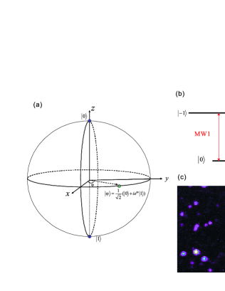
Figure 1: (color online) Bloch sphere and energy level for nitrogen vacancy center in diamond.(a) The states need to be cloned are in a specified form which are located in the equator of the Bloch sphere $|\psi\rangle=(|0\rangle+e^{i\phi}|1\rangle)/\sqrt{2}$. (b) Energy level of the NV center in diamond. (c) Two-dimension scanning confocal image of the sample. Bright spot circled is the NV center we investigate.

A NV center comprises a substitutional nitrogen atom instead of a carbon atom and an adjacent lattice vacancy. Experiments are carried out in a type Ib diamond nanocrystal from company Element Six. The average size of diamond nanocrystal is about 30 nm. Single NV defects in diamond are addressed by a home-built laser scanning confocal microscope system at room temperature [FIG. 1(c)]. A 532 nm continuous-wave laser modified by an acoustic optical modulator (AOM) with a rising edge of 10 ns is focused onto the sample with a microscope objective(numerical aperture=0.9). The fluorescence is also collected by the same objective, and passes through a 650 nm long-pass filter. Fluorescence signal is detected by a single photon counting module (SPCM, Perkin-Elmer) with a National Instruments counter 6602. Second order photon correlation function $g^{2}(\tau)$ of center A indicates that it is a single quantum emitter [FIG. 2(a)].

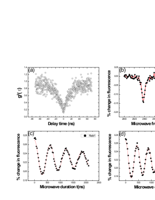
Figure 2: (color online) Second order photon correlation function, ESR spectrum, Rabi oscillations of two transitions. (a) Second order photon correlation function $g^{2}(\tau)$ of the NV center. (b) ESR spectrum of the NV center. Two main peaks correspond to m_s=1 and m_s=-1. (c) Rabi oscillations for the transition between m_s=0 and m_s=1. (d) Rabi oscillations for the transition between m_s=0 and m_s=-1.

The Hamiltonian with electron spin zero field splitting and the electron Zeeman interaction takes the form,

$$H=\textbf{S}\bar{D}\textbf{S}+\beta_{e}\vec{B}_{0}\bar{g}_{e}\textbf{S},$$ (1)

where $g_{e}$ and $\beta_{e}$ are the $g$ factor and Bohr magneton for electron, $\vec{B}_{0}$ is the applied magnetic field.

Experimentally, a microwave radiation is sent out by a copper wire of 20 $\mu$m diameter placed with a distance of 20 $\mu$m from the NV center. The Electron Spin Resonance (ESR) spectrum is shown in FIG. 2(b) as a function of the fluorescence change against the microwave frequency without external magnetic field, this is due to symmetry breaking of this NV center corresponding to a non-zero magnetic field. The two resonant frequencies correspond to the transitions of m_s=0 to m_s=1 and m_s=0 to m_s=-1. We denote the corresponding states as $|m_{s}=0\rangle_{p}$ and $|m_{s}=\pm 1\rangle_{p}$, where the subindex $p$ means those states are physical states to differ them from the logic qubits. In our experiment, the cloning processing is to transfer state $|\psi\rangle|0\rangle$ to two copies $|output\rangle=\frac{1}{\sqrt{2}}|00\rangle+\frac{1}{2}e^{i\phi}|01\rangle+\frac{1}{2}e^{i\phi}|10\rangle$. We use the encoding scheme: $-i|00\rangle\sim|m_{s}=-1\rangle_{p};|10\rangle\sim|m_{s}=0\rangle_{p};-i|01\rangle\sim|m_{s}=1\rangle_{p}$.

To control the electron spin state, first, a laser pulse initializes the spin state to $|m_{s}=0\rangle_{p}$; then the microwave pulses of weak power are used to manipulate the spin state; finally, the spin state is read out by the fluorescence intensity under a second laser excitation. The Rabi oscillation of the electron spin of single NV center is shown in FIG. 2(c) and (d), the scatter points are experiment data and each point is a statistical average result typically repeated $10^{5}$ times, the red line is the fitting using a function of a cosine with an exponential decay.

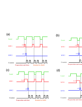
Figure 3: (color online)Scheme for quantum phase cloning. (a)A MW1 $\pi/2$ pulse creates $(|m_{s}=0\rangle_{p}+i|m_{s}=-1\rangle_{p})/\sqrt{2}$ state, then apply MW2 for another $\pi/2$ pulse for quantum phase cloning. After all we measure the standard Rabi oscillations for transition between $|m_{s}=0\rangle_{p}$ and $|m_{s}=-1\rangle_{p}$. (b) The same pulse sequence for the phase cloning, but we measure the Rabi oscillations for transition between $|m_{s}=0\rangle_{p}$ and $|m_{s}=1\rangle_{p}$. (c) A MW1 $3\pi/2$ pulse can create $(|m_{s}=0\rangle_{p}-i|m_{s}=-1\rangle_{p})/\sqrt{2}$ state, after phase cloning we measure Rabi oscillations with MW1. (d) The MW1 $3\pi/2$ pulse create $(|m_{s}=0\rangle_{p}-i|m_{s}=-1\rangle_{p})/\sqrt{2}$ state, after cloning we measure Rabi oscillations with MW2.

FIG. 3 shows the scheme for quantum phase cloning. The output state should be a superposition state $|output\rangle_{p}=\frac{1}{2}|m_{s}=0\rangle_{p}+i\frac{1}{2}|m_{s}=1\rangle_{p}+i\frac{1}{\sqrt{2}}|m_{s}=-1\rangle_{p}.$ The scheme for measure is by MW1 to confirm $|output\rangle_{p}$ is superposed by a pure state $\frac{1}{2}|m_{s}=0\rangle_{p}+i\frac{1}{\sqrt{2}}|m_{s}=-1\rangle_{p}$, and by MW2 to confirm the pure state form $\frac{1}{2}|m_{s}=0\rangle_{p}+i\frac{1}{2}|m_{s}=1\rangle_{p}$. Combination of those measured results indicate that the output is in form $|output\rangle_{p}$. By analyzing the experiment data, the exact form of the output state and the fidelity can be obtained. We then can repeat those experimental steps except that with different state preparation. The experimental results are shown in FIG. 4.

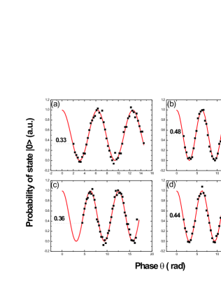
Figure 4: (color online)Measured results of the quantum phase cloning. (a) Red line is the standard dependence of probability of the state $|m_{s}=0\rangle_{p}$ on the phase of microwave pulse, by applying pulse sequence Figure 3(a), the black square is the experiment results for Rabi oscillations of transition with MW1, the start point of this curve determines the population probability at the state $|m_{s}=0\rangle_{p}$ is 33 %, theory is also around 33%. (b) Start point of the curve determines the probability at the state $|m_{s}=0\rangle_{p}$ is 48%, theory is 50% . (c) and (d) The start points of the curves determines the probability at the state $|m_{s}=0\rangle_{p}$ are 36% and 44%, theory are 33% and 50% .

The measured data by MW1 shows clearly Rabi oscillation which represents that the state of NV is in a superposed state. Also from the start point of Rabi oscillation, $\alpha$, the relative rate of fluorescence, we know that the measured state is in form $\sqrt{\alpha}e^{i\phi}|m_{s}=0\rangle_{p}+i\sqrt{1-\alpha}|m_{s}=-1\rangle_{p}$. Similarly with starting rate of fluorescence $\beta$ of MW2, we know the state is $\sqrt{\beta}|m_{s}=0\rangle_{p}+i\sqrt{1-\beta}e^{i\phi}|m_{s}=1\rangle_{p}$. The combination of those two results show that the NV center state should be the form

$$\sqrt{\alpha\beta}e^{i\phi}|m_{s}=0\rangle_{p}+i\sqrt{(1-\alpha)\beta}|m_{s}=-1\rangle_{p}$$

$$~{}~{}~{}+i\sqrt{(1-\beta)\alpha}e^{i\phi}|m_{s}=1\rangle_{p}$$ (2)

with normalization $1/\sqrt{\alpha+\beta-\alpha\beta}$. Using the experimental data in FIG. 4(a,b), we find two fidelities are $F_{1}=84.6\%$ and $F_{2}=86.1\%$, both are beyond the bound of the optimal fidelity of universal quantum cloning. By data in FIG. 4(c,d), we find the two fidelities of the two copies in output are $F_{1}=82.9\%$ and $F_{2}=87.1\%$, we find $F_{1}+F_{2}-\sqrt{(1-F_{1})(1-F_{2})}\approx 1.55$, which clearly larger than $1.5$ of the universal cloning Cerf . Thus phase cloning is better than the universal case. By average, we find the experimental cloning fidelity reaches $85.2\%$ which is very close to theoretical bound $85.4\%$ and apparently beyond the bound of the universal quantum cloning.

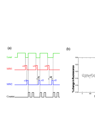
Figure 5: (color online) Quantum phase cloning for input state with different phases. (a) MW1 $\pi/2$ pulse is applied to create $(|m_{s}=0\rangle_{p}+i|m_{s}=-1\rangle_{p})/\sqrt{2}$ state, before applying MW2, we wait for time $jdt,j=1,2,...,dt=20ns,50ns$ so that state $(|m_{s}=0\rangle_{p}+i|m_{s}=-1\rangle_{p})/\sqrt{2}$ evolves freely to another state $(|m_{s}=0\rangle_{p}+e^{i\omega jdt}i|m_{s}=-1\rangle_{p})/\sqrt{2}$ with additional relative phase $\omega jdt$ depending on waiting time $jdt$ and rotating speed $\omega$ determined by environment, see thesis . (b) Experiment results show that with different waiting time periods within time scale 2 $\mu$s, after phase cloning operation, the intensity of fluorescence of the output state is stable which agrees with theory expectation.

A phase quantum cloning need the input state with an arbitrary phase. Experimental procedures are shown in FIG.5. This finishes the implementation of the whole quantum phase cloning.

In summary, we report the solid-state phase-covariant quantum cloning machine implementation in experiment at room temperature. Our observation shows that two microwave fields MW1 and MW2 can be combined to create an arbitrary superposition three-level state in quantum phase cloning processing and for other aims. This can be used as a basis for scalable, precisely controllable and measurable three-level quantum information devices.

This work is supported by NSFC (10974247, 10974251) and “973” programs (2009CB929103, 2010CB922904).

References

- (1) A. Gruber, A. Drabenstedt, C. Tietz, L. Fleury, J. Wrachtrup, and C. von Borczyskowski, Science 276, 2012 (1997).
- (2) P. Neumann, N. Mizuochi, F. Rempp, P. Hemmer, H. Watanabe, S. Yamasaki, V. Jacques, T. Gaebel, F. Jelezko, J. Wrachtrup, Science 320, 1326 (2008);
- (3) L. Viola, E. Knill, and S. Lloyd, Phys. Rev. Lett. 82, 2417 (1999).
- (4) W. Yao, R. B. Liu, and L. J. Sham, Phys. Rev. Lett. 98, 077602 (2007).
- (5) J. F. Du, X. Rong, N. Zhao, Y. Wang, J. Yang, and R. B. Liu, Nature 461, 1265 (2009).
- (6) B. Naydenov, F. Dolde, L. T. Hall, C. Shin, H. Fedder, Lloyd C. L. Hollenberg, F. Jelezko, and J. Wrachtrup, Phys. Rev. B 83, 081201(R) (2011).
- (7) J. R. Maze, P. L. Stanwix, J. S. Hodges, S. Hong, J. M. Taylor, P. Cappellaro, L. Jiang, M. V. G. Dutt, E. Togan, A. S. Zibrov, A. Yacoby, R. L. Walsworth, M. D. Lukin, Nature 455, 644 (2008).
- (8) J. M. Taylor, P. Cappellaro, L. Childress, L. Jiang, D. Budker, P. R. Hemmer, A. Yacoby, R. Walsworth, M. D. Lukin, Nature Physics 4, 810 (2008)
- (9) F. Shi, X. Rong, N. Xu, Y. Wang, J. Wu, B. Chong, X. Peng, J. Kniepert, R. S. Schoenfeld, W. Harneit, M. Feng, and J. F. Du, Phys. Rev. Lett. 105, 040504 (2010).
- (10) E. Togan, Y. Chu, A. S. Trifonov, L. Jiang, J. Maze, L. Childress, M. V. G, Dutt, A. S. Sorensen, P. R. Hemmer, A. S. Zibrov, M. D. Lukin, Nature 466, 730 (2010).
- (11) W.K.Wootters and W.H.Zurek, Nature 299, 802 (1982).
- (12) V. Scarani, S. Iblisdir, N. Gisin, and A. Acin, Rev. Mod. Phys. 77, 1225 (2005);
- (13) C. Vitelli, N. Spagnolo, L. Toffoli, F. Sciarrino, F. De Martini, Phys. Rev. Lett. 105, 113602 (2010).
- (14) H. W. Chen, D. W. Lu, G. Qin, X. Y. Zhou, X. H. Peng, and J. F. Du, Phys. Rev. Lett. 106, 180404 (2011).
- (15) C. H. Bennett and G. Brassard, in Proceedings of the IEEE International Conference on Computer, Systems, and Signal Processing, Bangalore, India (IEEE, New York, 1984), pp175-179.
- (16) D. Bruß, M. Cinchetti, G. M. D’Ariano, and C. Macchiavello, Phys. Rev. A 62, 012302 (2000).
- (17) H. Fan, K. Matsumoto, X. B. Wang, and M. Wadati, Phys. Rev. A 65, 012304 (2002).
- (18) J. F. Du, T. Durt, P. Zou, H. Li, L. C. Kwek, C. H. Lai, C. H. Oh, and A. Ekert, Phys. Rev. Lett. 94, 040505 (2005)
- (19) H. Chen, X. Zhou, D. Suter, and J. F. Du, Phys. Rev. A 75, 012317 (2007).
- (20) L. Childress, Ph. D thesis, Harvard University (2007).
- (21) N. J. Cerf, Phys. Rev. Lett. 84, 4497 (2000).