Robust limit on a varying proton-to-electron mass ratio from a single H₂ system

Abstract

Context. The variation of the dimensionless fundamental physical constant $\mu=m_{p}/m_{e}$ can be checked through observation of Lyman and Werner lines of molecular hydrogen in the spectra of distant QSOs. Only few, at present four, systems have been used for the purpose providing different results between the different authors.

Aims. Our intention is to asses the accuracy of the investigation concerning a possible variation of the fundamental physical constant $\mu=m_{p}/m_{e}$ and to provide more robust results. The goal in mind is to resolve the current controversy on variation of $\mu$ and devise explanations for the different findings. We achieve this not by another single result but by providing alternative approaches to the problem.

Methods. The demand for precision requires a deep understanding of the errors involved. Self-consistency in data analysis and effective techniques to handle unknown systematic errors are essential. An analysis based on independent data sets of QSO 0347-383 is put forward and new approaches for some of the steps involved in the data analysis are introduced. In this work we analyse two independent sets of observations of the same absorption system and for the first time we apply corrections for the observed offsets between discrete spectra mainly caused by slit illumination effects.

Results. Drawing on two independent observations of a single absorption system in QSO 0347-383 our detailed analysis yields $\Delta\mu/\mu=(15\pm(9_{\mathrm{stat}}+6_{\mathrm{sys}}))\times 10^{-6}$ at $z_{\mathrm{abs}}=3.025$. Based on the overall goodness-of-fit we estimate the limit of accuracy to $\approx$ 300 ms^-1, consisting of roughly 180 ms^-1due to the uncertainty of the fit and about 120 ms^-1allocated to systematics.

Conclusions. Current analyses tend to underestimate the impact of systematic errors. This work presents alternative approaches to handle systematics and introduces methods required for precision analysis of QSO spectra available in the near future.

1 Introduction

The Standard Model of particle physics (SMPP) is very successful and its predictions are tested to high precision in laboratories around the world. SMPP needs several dimensionless fundamental constants, such as coupling constants and mass ratios, whose values cannot be predicted and must be established through experiment (Fritzsch Fritzsch09 (2009)). Our confidence in their constancy stems from laboratory experiments over human time-scales but variations might have occurred over the 14 billion-year history of the Universe while remaining undetectably small today. Indeed, in theoretical models seeking to unify the four forces of nature, the coupling constants vary naturally on cosmological scales.

The proton-to-electron mass ratio, $\mu=m_{p}/m_{e}$ has been the subject of numerous studies. The mass ratio is sensitive primarily to the quantum chromodynamic scale. The $\Lambda_{QCD}$ scale should vary considerably faster than that of quantum electrodynamics $\Lambda_{QED}$. As a consequence, the secular change in the proton-to-electron mass ratio, if any, should be larger than that of the fine structure constant. This makes $\mu$ a very interesting target to search for possible cosmological variations of the fundamental constants.

The present value of the proton-to-electron mass ratio is $\mu$ = 1836.15267261(85) (Mohr et al. Mohr00 (2000)). Laboratory experiments by comparing the rates between clocks based on hyperfine transitions in atoms with a different dependence on $\mu$ restrict the time-dependence of $\mu$ at the level of $(\dot{\mu}/\mu)_{t_{0}}=(1.6\pm 1.7)\cdot 10^{-15}$ yr^-1 (Blatt et al. Blatt08 (2008)).

A probe of the variation of $\mu$ is obtained by comparing rotational versus vibrational modes of molecules as first suggested by Thompson (Thompson75 (1975)). The method is based on the fact that the wavelengths of vibro-rotational lines of molecules depend on the reduced mass, M, of the molecule. The energy difference between two consecutive levels of the rotational spectrum of a diatomic molecule scales with the reduced mass M, whereas the energy difference between two adjacent levels of the vibrational spectrum is proportional to $(M)^{1/2}$:

$$\nu=c_{e}+\frac{c_{v}}{\mu^{1/2}}+\frac{c_{r}}{\mu},$$ (1)

with $c_{e}$, $c_{v}$ and $c_{r}$ as constant factors for the electronic, vibrational and rotational contribution, respectively. Consequently, by studying the Lyman and Werner transitions of molecular hydrogen we may obtain information about a change in $\mu$. The observed wavelength $\lambda_{\mathrm{obs}}$ of any given line in an absorption system at the redshift $z$ differs from the local rest-frame wavelength $\lambda_{0}$ of the same line in the laboratory according to the relation

$$\lambda_{\mathrm{obs},i}=\lambda_{0,i}(1+z)(1+K_{i}\frac{\Delta\mu}{\mu}),$$ (2)

where $K_{i}$ is the sensitivity coefficient of the $i$th component computed theoretically for the Lyman and Werner bands of the H₂ molecule. Using this expression, the cosmological redshift of a line can be distinguished from the shift due to a variation of $\mu$.

This method was used to obtain upper bounds on the secular variation of the electron-to-proton mass ratio from observations of distant absorption systems in the spectra of quasars at several redshifts. The quasar absorption system towards QSO 0347-383 was first studied by us using high-resolution spectra obtained with the very large telescope/ultraviolet-visual echelle spectrograph (VLT/UVES) commissioning data we derived a first stringent bound at $(-1.8\pm 3.8)\cdot 10^{-5}$ (Levshakov et al. Levshakov02 (2002)). Subsequent measures of the quasar absorption systems of QSO 0347-382 and QSO 1232+082 provided hints for a variation $(2.4\pm 0.6)\cdot 10^{-5}$, i.e. at 3.5 $\sigma$ (Reinhold et al. Reinhold06 (2006); Ivanchik et al. Reinhold06 (2006, 2005); Ubachs et al. Ubachs07 (2007)). The new analysis used additional high-resolution spectra and updated laboratory data of the energy levels and of the rest frame wavelengths of the H₂ molecule.

However, more recently King et al. (King08 (2008)), Wendt & Reimers (Wendt08 (2008)) and Thompson et al. (Thompson09 (2009)) re-evaluated data of the same system and report a result in agreement with no variation. The more stringent limits on $\Delta\mu/\mu$ have been found at $\Delta\mu/\mu=(2.6\pm 3.0_{\rm stat})\times 10^{-6}$ from the combination of three H₂ systems (King et al. King08 (2008)) and a fourth one have provided $\Delta\mu/\mu=(+5.6\pm 5.5_{\rm stat}\pm 2.7_{\rm sys})\times 10^{-6}$ (Malec et al. Malec10 (2010)).

This work is motivated on one side by the use of a new data set available in the ESO data archive and previously overlooked and by numerous findings of different groups that partially are in disagreement witch each other. A large part of these discrepancies reflect the different methods of handling systematic errors. Evidently systematics are not yet under control or fully understood. We try to emphasize the importance to take these errors, in particular calibration issues, into account and put forward some measures adapted to the problem.

The bounds on the variation of $\mu$ are generally obtained by using the vibro-rotational transitions of molecular hydrogen, since H₂ is a very abundant molecule although very rarely seen in quasar absorbers. Only a few studies used other molecules since they are difficult to detect and measure accurately at large redshifts. In general these methods provide less stringent bounds on $\Delta\mu$ directly or bear a greater danger of nonuniform absorbers. Comparisons between the redshifts of H I 21cm (hyperfine) measured in the radio regime and ultraviolet resonance dipole transitions are sensitive to changes in $X\equiv g_{p}\alpha^{2}/\mu$ (see, i.e., Kanekar Kanekar2010 (2010)), which offers an important complementary verification of measured variations, although they sample different gas volumes.

One remarkable exception is the inverse spectrum of ammonia at radio wavelengths. A variation of $\Delta\mu/\mu$ can be tested through precise measurements of the relative radial velocities of narrow molecular lines observed in the cold interstellar molecular cores. This approach is based on a new method derived by Flambaum & Kozlov (Flambaum07 (2007)). Ammonia NH₃ is a molecule whose inversion transitions are very sensitive to changes in $\mu$ due to a tunneling effect. The sensitivity coefficient of the inversion transition NH${}_{3}(1,1)$ at $\nu=23.7$ GHz is almost two orders of magnitude more sensitive to $\mu$-variation than H₂ molecular rotational frequencies. By comparing the observed inversion frequency of NH₃(1,1) with a suitable rotational frequency of another molecule arising co-spatially with ammonia, a limit on the spatial variation of $\mu$ can be determined.

Ammonia has been detected in absorption in the main gravitational lenses of the quasars B 0218+357 and PKS 1830-211. Flambaum & Kozlov (Flambaum07 (2007)) combine the three detected NH₃ absorption spectra from B0218+357 with rotational spectra of CO, HCO⁺, and HCN to place a limit of (0.6$\pm$ 1.9) $\cdot$ 10^-6 for a look-back time of 6 Gyr (redshift z = 0.68). Accounting in detail for the velocity structure of the line profiles, Murphy et al. (2008) reanalyzed the ammonia data in combination with newly obtained high signal-to-noise rotational spectra of HCO⁺ and HCN. This yields $<$ 1.8 $\cdot$ 10^-6 at a 95% confidence level. Analyzing the ten NH₃ inversion lines and a similar number of rotational transitions from other molecules Henkel et al. (2009) obtain 10^-6 as a firm upper limit for a look-back time of 7 Gyr (z=0.89). However, the low number of NH₃ sources limit this method considerably, in particular for high redshifts.

Radio observations of OH lines at the Arecibo Telescope and the Westerbork Synthesis Radio Telescope yield $\Delta G/G=(-1.18\pm 0.46)\cdot 10^{-5}$ for a look back time of 2.9 Gyrs. $G$ is defined as $G\equiv g_{p}[\mu\alpha^{2}]^{1.85}$ and the results correspond to a change in $\alpha$, $\mu$ and/or $g_{p}$ (Kanekar et al. Kanekar2010b (2010)b).

In the following we will concentrate on the single H₂ system observed towards QSO 0347-383 to trace the proton-to-electron mass ration $\mu$ at high redshift ($z_{\mathrm{abs}}=3.025$). We intend to reach a robust estimation of the achievable accuracy with current data by comparing independent observation runs.

2 Data

2.1 Observations

QSO 0347-383 is a bright quasar (V $\approx$ 17.3) with z_em 3.23, which shows a Damped Lyman $\alpha$ system at z_abs = 3.0245. The hydrogen column density is of N(H I)= $5\cdot 10^{20}$ cm^-2 with a rich absorption-line spectrum (Levshakov et al. Levshakov02 (2002)). The z_abs = 3.025 DLA exhibits a multicomponent velocity structure. There are at least two gas components: a warm gas seen in lines of neutral atoms, H and low ions, and a hot gas where the resonance doublets of C IV and Si IV are formed. In correspondence of the cool component molecular hydrogen was first detected by Levshakov et al (2002b ) who identified 88 H₂ lines.

All works on QSO 0347-383 are based on the same UVES VLT observations in January 2002 (see Ivanchik et al. Ivanchik05 (2005)). The data used therein were retrieved from the VLT archive along with the MIDAS based UVES pipline reduction procedures. The slit width was 0.8″. The grating angle for the QSO 0347-383 observations had a central wavelength of 4300 Å. The images are 2$\times$2 binned. The 9 spectra were recorded during 3 nights with an exposure time of 4500 seconds each. Additional observational parameters are described in Ivanchick et al. (Ivanchik05 (2005)). The above mentioned data was recently carefully reduced again by Thompson et al. (Thompson09 (2009)). This work, however, is only in part based on this original reduced data.

Here we take into account additional observational data of QSO 0347-383 acquired in 2002 at the same telescope but not previously analyzed .

The UVES observations comprised of 6 $\times$ 80 minutes-exposures of QSO 0347-383 on several nights, thus adding another 28.800 seconds of exposure time. The journal of these observations as well as additional information is reported in Table 1. Three UVES spectra were taken with the DIC1 and setting 390+580 nm and three spectra with DIC2 and setting 437+860, thus providing blue spectral ranges between 320-450 and 373-500 nm respectively. We note that QSO 0347-383 has no flux below 370 nm due to the Lyman discontinuity of the z_abs=3.023 absorption system. The slit width was set to 1″  for all observations providing a Resolving Power of $\approx$ 40 000. The different slit widths and hence different resolutions of the observation runs pose no problem since all data are analyzed separately during the fit. The seeing was varying in the range between 0.5″ to 1.4″ as measured by DIMM but generally is better than this at the telescope. The CCD pixels were binned by 2$\times$2 providing an effective 0.027-0.030 Å pixel, or 2.25 kms^-1at 400 nm along dispersion direction.

Table 1: Journal of the observations

Date	Time	$\lambda$	Exp(sec)	Seeing (arcsec)	airmass	S/N (mean)
2002-01-13	03:42:54	390	4800	1.7	1.5	20
2002-01-14	02:13:24	390	4800	1.0	1.2	28
2002-01-15	00:43:32	437	4800	0.96	1.0	67
2002-01-18	03:25:04	437	4800	1.63	1.4	49
2002-01-24	02:20:14	437	4800	1.07	1.7	29
2002-02-02	01:33:58	390	4800	0.5	1.2	37

2.2 Reduction

The standard UVES pipeline has been followed for the data reduction. This includes sky subtraction and optimal extraction of the spectrum. Typical residuals of the wavelength calibrations were of $\approx$ 0.5 mÅ  or $\approx$ 40 ms^-1 at 400 nm. The spectra were reduced to barycentric coordinates and air wavelengths have been transformed to vacuum by means of the dispersion formula by Edlen (Edlen66 (1966)). Proper calibration and data reduction will be the key to detailed analysis of potential variation of fundamental constants. The influence of calibration issues on the data quality is hard to measure and the magnitude of the resulting systematic error is under discussion. The measurements rely on detecting a pattern of small relative wavelength shifts between different transitions spread throughout the spectrum. Normally, quasar spectra are calibrated by comparison with spectra of a hollow cathode thorium lamp rich in unresolved spectral lines. However several factors are affecting the quality of the wavelength scale. The paths for ThAr light and quasar light through the spectrograph are not identical thus introducing small distortions between ThAr and quasar wavelength scales. In particular differences in the slit illuminations are not traced by the calibration lamp. Since source centering into the slit is varying from one exposure to another this induce an offset in the zero point of the scales of different frames which could be up to few hundred of ms^-1. In section 3.1 we provide an estimate of these offsets which result of a mean offset of 168 m s^-1 as well as a procedure to avoid this problem. Laboratory wavelengths are know with limited precision which is varying from line to line from about 15 ms^-1of the better known lines to more than 100 ms^-1for the more poorly known lines (Murphy et al. Murphy08 (2008) and Thompson et al. Thompson09 (2009)). However, this is the error which is reflected in the size of the residuals of the wavelength calibration. Iodine cell based calibration cannot be applied directly in the case of QSO 0347-383 since at a redshift of $z\approx 3$ all observed lines lie outside the range of Iodine lines which cover about 5 000-6 000 Å. Additionally, at the given level of continuum contamination due to Lyman-$\alpha$ forest at such redshifts a super-imposed spectrum of the iodine cell is not desirable.

Effects of this kind have been investigated at the Keck/HIRES spectrograph by comparing the ThAr wavelength scale with one established from I2-cell observations of a bright quasar by Griest et al. (Griest10 (2010)). They found both absolute and relative wavelength offsets in the Keck data reduction pipeline which can be as large as 500 - 1 000 ms^-1for the observed wavelength range. Such errors would correspond to $\Delta\mathrm{\lambda}\approx 10-20\,\mbox{m\AA}$ and exceed by one order of magnitude presently quoted errors (Thompson et al. Thompson09 (2009)). Examination of the UVES spectrograph at the VLT carried out via solar spectra reflected on asteroids with known radial velocity showed no such dramatic offsets being less than $\approx$ 100 ms^-1( Molaro et al.Molaro08b (2008)) but systematic errors at the level of few hundred ms^-1have been revealed also in the UVES data by comparison of relative shifts of lines with comparable response to changes of fundamental constants (Centurion et al. Centurion09 (2009)). These examples well show that current $\Delta\mu/\mu$-analysis based on quasar absorption spectra at the level of a few ppm enters the regime of calibration induced systematic errors. While awaiting a new generation of laser-comb-frequency calibration, today’s efforts to investigate potential variation of fundamental physical constants require factual consideration of the strong systematics.

We note also that the additional observations considered here were taken for other purposes and the ThAr lamps are taken during daytime, which means several hours before the science exposures and likely under different thermal and pressure conditions. However, in the present work we bypass the possibility of different zero points of the different images via the seldom case of independent observations. Instead of co-adding all the spectra we compute first the global velocity shifts between the spectra with the procedure described in the following section and we also utilize the whole uncertainties coming from the wavelength accuracies as part of the analysis procedure.

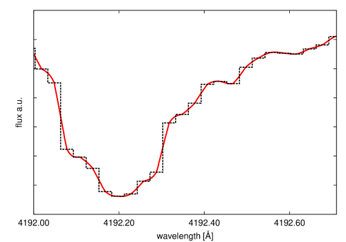
Figure 1: Example region of the QSO 0347-383 spectrum showing the recorded flux (dashed) and its interpolation via a polynomial using Neville’s algorithm to conserve the local flux.

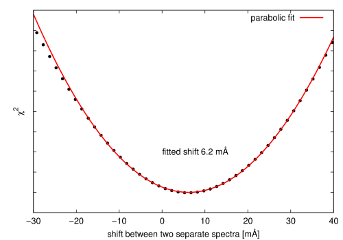
Figure 2: Exemplary plot of the sub-pixel cross-correlation. The resulting shift is ascertained via parabolic fit. In this case the two spectra are in best agreement with a relative shift of 6.2 $\pm$ 0.5 mÅ.

2.3 Noise level

The UVES data reduction procedure deliver the error spectrum along the optimally extracted spectrum. The given error in flux of all 15 spectra was tested against the zero level noise in saturated areas. A broad region of saturated absorption is available near $3906\AA$ in the observers frame. Statistical analysis revealed a variance corresponding to $\sim$120% of the given error on average for the 15 spectra. This means that normally errors that rely to the standard extracted routine are probably underestimated by a comparable amount. In particular we compared the standard deviation of the flux between $3903.8\AA$ and $3908.7\AA$ (roughly 160 samples) with the average of the specified error for that range. In our analysis for each of the spectra the calculated correction factor was applied.

3 Preprocessing

3.1 Relative shifts of the 15 spectra

Prior to further data processing the reduced spectra are reviewed in detail. The first data set (henceforward referred to as set A) consists of nine separate spectra observed between 7th and 9th of January in 2002. The second set of 6 spectra (B) was obtained between January 13th and February 2nd in 2002 (see Table 1).

Due to slit illumination effects and grating motions the individual spectra are subject to small shifts – commonly on sub-pixel level – in wavelength. These shifts will be particularly crucial in the process of co-addition of several exposures. To estimate these shifts all spectra were interpolated by a polynomial using Neville’s algorithm to conserve the local flux (see Fig. 1). The resulting pixel step on average is $1/20$ of the original data. Each spectrum was compared to the others. For every data point in a spectrum the pixel with the closest wavelength was taken from a second spectrum. Their deviation in flux was divided by the quadratic mean of their given errors in flux. This procedure was carried out for all pixels inside certain selected wavelength intervals resulting in a mean deviation of two spectra. The second spectrum is then shifted against the first one in steps of $\sim 1.5$ mÅ. The run of the discrepancy of two spectra is of parabolic nature with a minimum at the relative shift with the best agreement. Fig. 2 shows the resulting curve with a parabolic fit. In this exemplary case the second spectrum shows a shift of 6.2 mÅ in relation to the reference spectrum. The clean parabolic shape verifies the approach. Table 2 shows the corresponding offsets for the 15 spectra. The offsets between the exposures are relevant with a peak to peak excursion up to almost 800 ms^-1. The average deviation is 2.3 mÅor 170 ms^-1at 400 nm. For further analysis in this paper all the 15 spectra are shifted to their common mean, which is taken as an arbitrary reference position. To avoid areas heavily influenced by cosmic events or areas close to overlapping orders only certain wavelength intervals were taken into account, namely the regions 3877-3886 Å, 3986-4027 Å, 4145-4175 Å and 4216-4240 Å  (referred to as 1-4 in Table 2). The individual intervals show no significant differential shifts and their combined wavelength range was used to obtain a more robust mean shift between two spectra. To estimate the error of the given shifts, the routine was carried out for all spectrum-combinations and the resulting shifted spectra were checked for shifts again. We estimate the error per shift to be of 38 ms^-1based on the deviation of the individual shifts of four wavelength intervals. Section 4.3 illustrates its influence on the data analysis with respect to the previous analysis of the data set A, in which this effect was not considered.

Table 2: Relative shifts of the observed spectra to their common mean. Spectra A1-A9 correspond to the observations of Program ID 68.A-0106, spectra B1-B6 to Program ID 68.B-0115(A), respectively. shift 1-4 represent the individual offsets for the four selected wavelength intervals.

ID	shift 1	shift 2	shift 3	shift 4	shift 1-4	$\sigma_{1-4}$
	(ms-1)	(ms-1)	(ms-1)	(ms-1)	(ms-1)	(ms-1)
A1	-243	-239	-240	-269	-203	13
A2	-163	-112	-52	-107	-135	39
A3	42	92	95	105	116	24
A4	-46	-107	-29	-45	-61	30
A5	222	295	182	223	268	41
A6	15	-75	-101	11	-31	51
A7	-189	-312	-212	-258	-249	47
A8	129	11	87	112	65	45
A9	305	192	218	229	249	42
B1	114	70	85	30	84	30
B2	524	439	563	501	496	45
B3	19	17	50	86	39	28
B4	-286	-417	-290	-388	-339	58
B5	129	11	24	-23	30	57
B6	-101	-120	-173	-111	-158	28
average standard deviation						38

3.2 Selection of lines and line fitting

The selection of suitable H₂ features for the final analysis is rather subjective. As a matter of course all research groups cross-checked their choice of lines for unresolved blends or saturation effects. The decision whether a line was excluded due to continuum contamination or not, however, relied mainly on the expert knowledge of the researcher and was only partially reconfirmed by the ascertained uncertainty of the final fitting procedure. This work puts forward a more generic approach adapted to the fact that we have two distinct observations of the same object.

In this paper each H₂ signature is fitted with a single component. The surrounding flux is fit by a ploynomial and the continuum is rectified accordingly. This approach is tested and verified in Wendt & Reimers (Wendt08 (2008)), however lines near saturated or steeply descending areas should be avoided. A selection of 52 (in comparison with 68 lines for that system by King et al. (King08 (2008))) lines is fitted separately for each dataset of 9 (A) and 6 (B) exposures, respectively. In this selection merely blends readily identifiable or emerging from equivalent width analysis are excluded. Each rotational level is fitted with conjoined line parameters except for redshift naturally. A common column density $N$ and broadening parameter $b$ corresponds to each of the observed rotational levels (in this case $J=1,2,3$).

The data are not co-added but analyzed simultaneously via the fitting procedure introduced in Quast et al. (Quast05 (2005)). In principle each set of parameters (line centroid, broadening parameter, column density, coefficients of the continum polynomial) drawn from a large parameter space is tested in all individual spectra and judged by a weighted $\chi^{2}$. The standard deviations of line positioning are provided by the diagonal elements of the scaled covariance matrix, a procedure described in detail in the above mentioned paper by Quast et al. and verified, i.e., in Wendt et al. (Wendt08 (2008)). For each of the 52 lines there are two resulting fitted redshifts or observed wavelengths, respectively, with their error estimates. To avoid false confidence, the single lines are not judged by their error estimate but by their difference in wavelength between the two data sets in relation to the combined error estimate. Fig. 5 shows this dependency. The absolute offset $\Delta\mathrm{\lambda_{\mathrm{effective}}}$ to each other is expressed in relation to their combined error given by the fit:

$$\Delta\lambda_{\sigma_{\Sigma 1,2}}=\frac{\Delta\lambda_{\mathrm{effective}}}{\sqrt{\sigma^{2}_{\lambda_{1}}+\sigma_{\lambda_{2}}^{2}}}.$$ (3)

Fig. 5 reveals notable discrepancies between the two datasets, the disagreement is partially exceeding the 5-$\sigma$ level. Since the fitting routine is known to provide proper error estimates (Quast et al. Quast05 (2005); Wendt et al. Wendt08 (2008)), the dominating source of error in the determination of line positions is due to systematic errors. This result indicates calibration issues of some significance at this level of precision. The comparison of two independent observation runs reveals a source of error that cannot be estimated by the statistical quality of the fit alone. For further analysis only lines that differ by less than 3 $\sigma$ are taken into account. This criterion is met by 36 lines. Fig. 6 shows three examplary H₂ features corresponding to the transitions L5R1, L5P1, L5R2. All have similar sensitivity towards changes in $\mu$. L5P1 fails the applied self consistency check between the two data sets and is excluded in the further analysis. Table 4 lists the excluded lines.

It is noteworthy that line selections of this absorption system by other groups diverge from each other by a large amount. King et al. (King08 (2008)) processed a total of 68 lines. By reconstructing the continuum flux with additionally fitted lines of atomic hydrogen they felt confident not to care about the relative position of the H₂ features next to the Lyman-$\alpha$ forrest. Fitting H₂ features as single lines, however, is affected by the surrounding flux and its nature as simulations have shown (Wendt & Reimers Wendt08 (2008)). Thompson et al. (Thompson09 (2009)) selected 36 lines for analysis of which differs from our semi-automatical choice of lines by almost 40%.

Hence, the different findings arise through in large parts independent analysis. Different approaches, line selections and in the end applied methods contribute to a more solid constraint on variation of fundamental constants. This variety is mandatory to understand contradicting findings, not only in case of the proton-to-electron mass ratio. Table 3 report the molecular line position and relative errors. Figure 3 plots the results of this paper, Ubachs et al. (Ubachs07 (2007)) and Thompson et al. (Thompson09 (2009)), who published the individual fit parameters. The redshifts derived are of 3.0248969 (56), 3.0248988(29) and 3.0248987(61) for this paper, Ubachs et al (2007) and Thompson (2009) respectively, which is not surprising being based at least partially on the same data. All three analysis are based on the same source for sensitivity coefficients. The distribution of positioning errors for the mentioned works is illustrated in Figure 4. The three sets of measure show a significant scatter around the mean quite in excess of the error in line position which is suggestive of the presence of systematic errors.

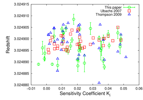
Figure 3: Final results in redshift vs. sensitivity coefficient $K_{i}$ for this paper (circles), Ubachs et al. Ubachs07 (2007) (squares) and Thompson et al. Thompson09 (2009) (triangles).

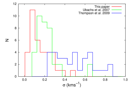
Figure 4: Line positioning errors in kms^-1  for this paper (solid), Ubachs et al. Ubachs07 (2007) (dashed) and Thompson et al. Thompson09 (2009) (dotted), binned to 50 ms^-1.

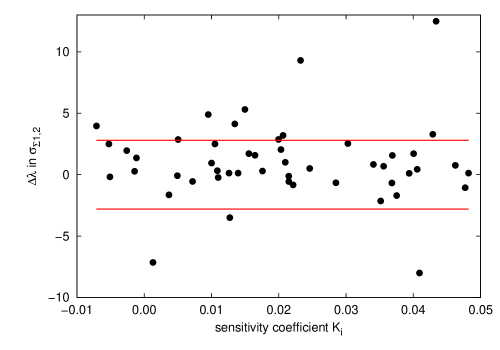
Figure 5: Selection of 52 apparently reasonable lines to be fitted separately for each dataset of 9 and 6 exposures, respectively. Their absolute offset $\Delta\lambda_{\mathrm{effective}}$ to each other is expressed in relation to their combined error given by the fit (see Eq.3). The dashed lines border the $3\sigma$ domain.

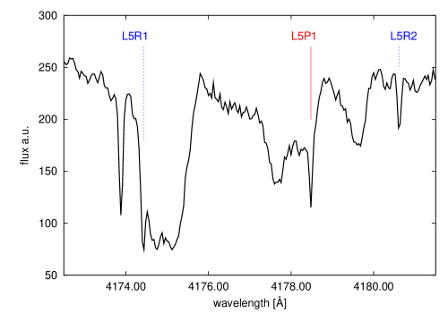
Figure 6: Part of the co added spectrum near 4176Å. The data however, were not co added for the fit. L5R1 and L5R2 match the 3-$\sigma$ criterion, L5P1 does not.

The chosen $\Delta\lambda$ criterium for line selection permits evaluation of the self-consistency of a line positioning via fit for the involved data. While the availability of two independent observations on short time scale is rather special, it illustrates one applicable modality to avoid relying on the fitting apparatus alone.

4 Results

For the final analysis the selected 36 lines are fitted in all 15 shifted, error-scaled spectra simultaneously. The result of an unweighted linear fit corresponds to $\Delta\mu/\mu=(15\pm 16)\times 10^{-6}$ over the look-back time of $\sim 11.5$ Gyr for $z_{\mathrm{abs}}=3.025$. Fig. 7 shows the resulting plot. The complete list of lines is shown in Table 3. The approach to apply an unweighted fit is a consequence of the unknown nature of the prominent systematics. The graphed scatter in redshift can not be explained by the given positioning errors alone. The likeliness of the data with the attributed error being linearly correlated is practically zero. The fit to the data is not self-consistent. For this work the calibration errors and the influence of unresolved blends are assumed to be dominant in comparison to individual fitting uncertainties per feature. For the following analysis the same error is adopted for each line. With an uncertainty in redshift of $1\times 10^{-6}$ we obtain: $\Delta\mu/\mu=(15\pm 6)\times 10^{-6}$. However the goodness-of-fit is below 1 ppm and is not self consistent. The goodness of fit of a statistical model describes how well it fits a set of observations. A linear model with the given parameters does not represent the observed data sample very well. The apparent discrepancies between model and data including their errorbars shown in Figure 7 are extremely unlikely (below one part per million) to be chance fluctuations. Judging by that and Fig. 7, a reasonable error in observed redshift should at least be in the order of $4-5\times 10^{-6}$. The weighted fit gives: $\Delta\mu/\mu=(15\pm 14)\times 10^{-6}$.

This approach is motivated by the goodness-of-fit test:
$Q(\chi^{2}|\nu)$ is the probability that the observed chi-square will exceed the value $\chi^{2}$ by chance even for a correct model, $\nu$ is the number of degrees of freedom. Given in relation to the incomplete gamma function:

$$Q(\chi^{2}|\nu)=\Gamma\left(\frac{\nu}{2},\frac{\chi^{2}}{2}\right).$$ (4)

Assuming a gaussian error distribution, $Q$ gives a quantative measure or the goodness-of-fit of the model. If $Q$ ist very small for some particular data set, then the apparent discrepancies are unlikely to be chance fluctuations that would be expected for a gaussian error distribution. Much more probably either the model is wrong or the size of the measurement errors is larger than stated. However, the chi-square probability $Q$ does not directly measure the credibility of the assumption that the measurement errors are normally distributed. In general, models with $Q<0.001$ can be considered inacceptable. In this case the model is given and hence the low probability is due to underestimated errors in the data. Solely for given errors of $\approx$ 300 ms^-1, corresponding to $\approx 4\times 10^{-6}$ in redshift for QSO 0347-383 the goodness-of-fit parameter $Q$ exceeds $0.001$. The scale of the error appears to be $\approx$ 300 ms^-1to achieve a self-consistent fit to the data.

For the data on QSO 0347-383 this corresponds to an error in the observed wavelength of roughly $4\mbox{m\AA}$, which is notably larger than the estimated errors for the individual line fits which ranges from $0.5\mbox{m\AA}$  to $6.5\mbox{m\AA}$  with an average of $2.5\mbox{m\AA}$ ($\approx$ 180 ms^-1). The systematic error contributes an uncertainty of about $2\mbox{m\AA}$ on average. The immediate calibration errors are in the order of 50 ms^-1for set B and presumably slightly larger for set A. Figure 8 plots the data with errorbars corresponding to 180ms^-1  and the total of 300 ms^-1.

The final result can be subdivided as:
$\Delta\mu/\mu=\left(15\pm(9_{\mathrm{stat}}+6_{\mathrm{sys}})\right)\times 10^{-6}$.

The comparably high scatter in Figure 7 can partially be attributed to the approach to fit single H₂ components with a polynomial fit to the continuum. In special cases, contaminated flux bordering a H₂ signature can introduce additional uncertainty in positioning therefore checks for self-consistency and systematics are of utmost importance.

The determination of the different errors involved is on a par with the actual result.

We believe that this result represents the limit of accuracy that can be reached with the given data set and the applied methods for analysis. The presented method yields a null result. The recent work by Thompson et al. (Thompson09 (2009)) stated $\Delta\mu/\mu=(-28\pm 16)\times 10^{-6}$ for a weighted fit based on the same system in QSO 0347-383. The therein stated error reflects the statistical uncertainty alone.

Note, that the given systematics of $2.7$ppm for Keck/HIRES data given in Malec et al. (Malec10 (2010)) are in first approximation estimated by the observed $\sim$500 ms^-1 peak-to-peak intra-order value reduced according to the number of molecular transitions observed, i.e. $\sim 500\,\mbox{ms${}^{-1}$}/\sqrt{93}\approx 52\,\mbox{ms${}^{-1}$}$.

This work proposes to take alternative approaches into account when operating that close to the limits of several involved systems. The presented method was applied to the known QSO 0347-383 data for two main reasons:

• As an example to put forward alternative strategies.

• A stand-alone determination of $\Delta\mu/\mu$ based on QSO 0347-383 to back up current null-results and consequential constraints.

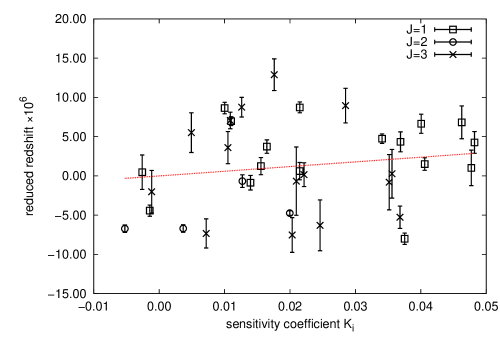
Figure 7: The unweighted fit for QSO 0347-383 corresponds to $\Delta\mu/\mu=(15\pm 16)\times 10^{-6}$. The error bars correspond merely to the fitting uncertainty in the order of 180 ms^-1  on average. Note, that at such a high scatter $z_{Ki=0}$ differs from $\bar{z}$ by less than 1 $\sigma_{\mathrm{z}}$.

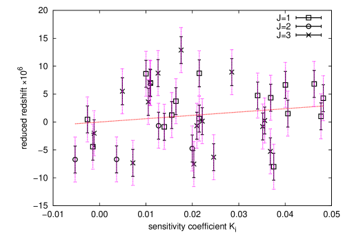
Figure 8: Data identical to Fig.7. The errorbars represent the average positioning error (solid) and the additional systematic error (dotted) of $\approx$ 180 ms^-1  and $\approx$ 120 ms^-1, respectively.

Table 3: QSO 0347-383 Line List

Line ID	K factor	Obs. wavelength [Å]	pos. error [Å]	Lab. wavelength [Å]	pos. error [kms-1]	redhisft
L14R1	0.0462	3811.5038	0.0031	946.9804	0.247	3.0249025
W3Q1	0.0215	3813.2825	0.0012	947.4219	0.091	3.0249043
W3P3	0.0210	3830.3795	0.0064	951.6719	0.499	3.0248950
L13R1	0.0482	3844.0442	0.0023	955.0658	0.181	3.0248999
L13P1	0.0477	3846.6271	0.0039	955.7083	0.306	3.0248966
W2Q1	0.0140	3888.4352	0.0017	966.0961	0.128	3.0248948
W2Q2	0.0127	3893.2050	0.0013	967.2811	0.099	3.0248951
L12R3	0.0368	3894.7939	0.0019	967.6770	0.149	3.0248904
W2Q3	0.0109	3900.3288	0.0013	969.0492	0.097	3.0249028
L10R1	0.0406	3952.7477	0.0015	982.0742	0.110	3.0248972
L10P1	0.0400	3955.8160	0.0020	982.8353	0.154	3.0249022
L10R3	0.0356	3968.3977	0.0040	985.9628	0.302	3.0248960
L10P3	0.0352	3975.6657	0.0055	987.7688	0.412	3.0248950
W1Q2	0.0037	3976.4877	0.0007	987.9745	0.054	3.0248890
L9R1	0.0375	3992.7546	0.0013	992.0164	0.098	3.0248877
L9P1	0.0369	3995.9594	0.0022	992.8096	0.167	3.0249000
L8R1	0.0341	4034.7699	0.0011	1002.4521	0.085	3.0249004
L8P3	0.0285	4058.6575	0.0034	1008.3860	0.255	3.0249046
W0R2	-0.0052	4061.2132	0.0006	1009.0249	0.047	3.0248890
L7P3	0.0246	4103.3836	0.0052	1019.5022	0.379	3.0248894
L6R3	0.0221	4141.5640	0.0023	1028.9866	0.168	3.0248960
L6P3	0.0203	4150.4349	0.0034	1031.1926	0.245	3.0248882
L5R1	0.0215	4174.4204	0.0019	1037.1498	0.139	3.0248963
L5R2	0.0200	4180.6152	0.0005	1038.6903	0.034	3.0248910
L5R3	0.0176	4190.5690	0.0031	1041.1588	0.218	3.0249086
L4R1	0.0165	4225.9822	0.0016	1049.9597	0.111	3.0248994
L4P1	0.0156	4230.2974	0.0021	1051.0325	0.151	3.0248969
L4R3	0.0126	4242.1531	0.0018	1053.9761	0.126	3.0249045
L4P3	0.0105	4252.1911	0.0030	1056.4714	0.211	3.0248994
L3R1	0.0110	4280.3234	0.0010	1063.4601	0.071	3.0249027
L3P1	0.0100	4284.9349	0.0014	1064.6054	0.097	3.0249043
L3R3	0.0072	4296.4822	0.0028	1067.4786	0.198	3.0248884
L3P3	0.0049	4307.2114	0.0040	1070.1409	0.276	3.0249012
L2P3	-0.0011	4365.2399	0.0046	1084.5603	0.318	3.0248937
L1R1	-0.0014	4398.1291	0.0015	1092.7324	0.100	3.0248913
L1P1	-0.0026	4403.4456	0.0042	1094.0520	0.283	3.0248961
average			0.0025		0.184

Table 4: Excluded lines

Line ID	K factor	Lab. wavelength [$\AA$]
L12P2	0.0434	966.2755
L11P1	0.0429	973.3345
L11P2	0.0409	975.3458
W0Q2	-0.0071	1010.9384
L7R1	0.0303	1013.4370
L6R2	0.0245	1026.5283
L6P2	0.0232	1028.1058
L5P1	0.0206	1038.1571
L5P2	0.0186	1040.3672
L4R2	0.0150	1051.4985
L4P2	0.0135	1053.2843
L3R2	0.0095	1064.9948
L2R1	0.0050	1077.6989
L2R3	0.0013	1081.7113

4.1 Uncertainties in the sensitivity coefficients

At the current level of precision, the influence of uncertainties in the sensitivity coefficients $K_{i}$ is minimal. It will be of increasing importance though when wavelength calibration can be improved by pedantic demands on future observations. Eventually Laser Frequency Comb calibration will allow for practically arbitrary precision and uncertainties in the calculations of sensitivities will play a role. Commonly the weighted fits neglects the error in $K_{i}$.

Effective analysis in the future involves consideration of the error budget of the sensitivity coefficients. The $\chi^{2}$ merit function for the generic case of a straight-line fit with errors in both coordinates is given by:

$$\chi^{2}(a,b)=\sum^{N-1}_{i=0}\frac{(y_{i}-a-bx_{i})^{2}}{\sigma^{2}_{yi}+b^{2}\sigma^{2}_{xi}}$$ (5)

and can be solved numerically with valid approximations (Lybanon Lybanon84 (1984)).

At the current level even an error in $K_{i}$ of about 10% merely has an impact on the error estimate in the order of a few $10^{-6}$, as resulted from simulations. The factual errors are expected to be in the order of merely a few percent (Ubachs et al. Ubachs07 (2007)), yet they might contribute to the precision of future analysis.

Alternatively the uncertainties in $K_{i}$ can be translated into an uncertainty in redshift via the previously fitted slope:

$$\sigma_{z_{i\,\mathrm{total}}}=\sigma_{z_{i}}+b\times\sigma_{K_{i}}\hskip 14.22636pt\mathrm{with}\hskip 14.22636ptb=(1+z_{\mathrm{abs}})\frac{\Delta\mu}{\mu}.$$ (6)

The results of this ansatz are similar to the fit with errors in both coordinates and in general this is simpler to implement.

Another possibility is to apply a gaussian error to each sensitivity coefficient and redo the normal fit multiple times with alternating variations in $K_{i}$. Again, the influence on the error-estimate is in the order of 1 ppm. The different approaches to the fit allow to estimate its overall robustness as well.

4.2 Individual line pairs

$\Delta\mu/\mu$ can also be obtained by using merely two lines that show different sensitivity towards changes in the proton-to-electron mass ratio. Another criterion is their separation in the wavelength frame to avoid pairs of lines from different ends of the spectrum and hence in particular error-prone. Several tests showed that a separation of $\Delta\lambda\leq 110\,\AA$ and a range of sensitivity coefficients $K_{1}-K_{2}\geq 0.02$ produces stable results that do not change any further with more stringent criteria. Pairs that cross two neighboring orders ($\sim 50\AA$) show no striking deviations either. Fig. 9 graphs the different values for $\Delta\mu/\mu$ derived from 52 line pairs that match the aforementioned criteria. Note, that a single observed line contributes to multiple pairs. The gain in statistical significance by this sorting is limited as pointed out by Molaro et al. (Molaro08 (2008)). Their average value yields $\Delta\mu/\mu=6\pm 12\times 10^{-6}$. The scatter is then related to uncertainties in the wavelength determination which is mostly due to calibration errors. The standard error is $8\times 10^{-6}$.

The approach to use each observed line only once in the analysis is plotted in Fig. 9 as filled squares. The pairs to derive $\Delta\mu/\mu$ from were constructed by grouping the line with the highest sensitivity value together with the line corresponding to the lowest value for K_i and so on with the remaining lines. The distance in wavelength space between the two lines was no critierum and it ranges from 20Å  to 590Å  (see Table 5). Without reutilization of lines, 11 pairs with a coverage in sensitivity of $\Delta$K${}_{i}\geq 0.02$ were found.

Evidently the usage of lines with comparably large distances in the spectrum has no influence on the results.

Table 5: Grouping all observed lines into 17 pairs of maximum K_i sensitivity not considering their separation in wavelength space (rightmost column).

Line 1	Line 2	$\Delta\mu/\mu$	$\Delta$Ki	$\Delta\lambda$ [$\AA$]
W0R2	L13R1	50.5 $\times 10^{-6}$	0.0535	-217.169
L1P1	L13P1	2.7 $\times 10^{-6}$	0.0503	-556.818
L1R1	L14R1	58.6 $\times 10^{-6}$	0.0477	-586.625
L2P3	L10R1	20.9 $\times 10^{-6}$	0.0417	-412.492
W1Q2	L10P1	90.4 $\times 10^{-6}$	0.0364	-20.672
L3P3	L9R1	-103.0 $\times 10^{-6}$	0.0326	-314.457
L3R3	L9P1	97.6 $\times 10^{-6}$	0.0297	-300.523
L3P1	L12R3	-128.9 $\times 10^{-6}$	0.0268	-390.141
L4P3	L10R3	-33.9 $\times 10^{-6}$	0.0251	-283.793
W2Q3	L10P3	-79.4 $\times 10^{-6}$	0.0243	75.337
L3R1	L8R1	-24.0 $\times 10^{-6}$	0.0231	-245.554
L4R3	L8P3	3.1 $\times 10^{-6}$	0.0159	-183.496
W2Q2	L7P3	-120.0 $\times 10^{-6}$	0.0119	210.179
W2Q1	L6R3	34.0 $\times 10^{-6}$	0.0082	253.129
L4P1	W3Q1	312.7 $\times 10^{-6}$	0.0059	-417.015
L4R1	L5R1	-154.6 $\times 10^{-6}$	0.0050	-51.562
L5R3	W3P3	-996.4 $\times 10^{-6}$	0.0034	-360.190

4.3 Influence of the preprocessing

Section 3.1 describes the initial shift to a common mean of all 15 spectra. The complete analysis was redone with error-scaled but unshifted spectra and the ascertained line positions of both runs compared. Fig. 10 shows the difference for each H₂ line in mÅ over the corresponding sensitivity coefficients $K_{i}$. The plotted line is a straight fit. Clearly the slope is dominated by three individual lines whose fitted centroids shifted up to $5.5$ mÅ due to the preprocessing. These three lines in particular produce a trend towards variation in $\mu$ when grating shifts and other effects are not taken into account. This single-sided trend probably occurred by mere chance but at such low statistics it influences the final result. Similar effects might have introduced trends of non-zero variation in former works (i.e., Ivanchik et al. Ivanchik05 (2005); Reinhold et al. Reinhold06 (2006)).

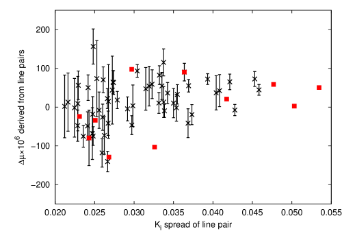
Figure 9: $\Delta\mu/\mu$ derived from individual line pairs (52) which are separated by less than 110 Å  and show a difference in sensitivity of more then $0.02$. The errorbars reflect the combined positioning error of the two contributing lines. The weighted fit corresponds to $\Delta\mu/\mu=(6\pm 12)\times 10^{-6}$.
The filled squares graph 11 line pairs, selected to give the largest difference in sensitivity ($\geq 0.02$) towards variation in $\mu$ (See Table 5).

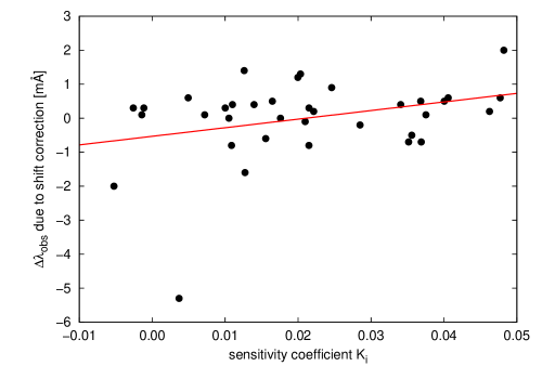
Figure 10: Variation in fitted positions for all lines with and without initial correction for shifts in between the 15 spectra. The slope of the fit is dominated by three lines.

- (1) Blatt, S. and Ludlow, A. D. and Campbell, G. K., et al. 2008, Phys. Rev. Lett., 100, 14
- (2) Centurión, M. and Molaro, P. and Levshakov, S. 2009, ArXiv 0910.4842
- (3) Edlén, B. 1966, Metrologia, 2, 71
- (4) Flambaum, V. V. and Kozlov, M. G. 2007, Phys. Rev. Lett., 98, 24
- (5) Fritzsch, H. 2009, arXiv:0902.2989
- (6) Griest, K. and Whitmore, J. B., Wolfe, A. M., et al. 2010, ApJ, 708, 158
- (7) Ivanchik, A. and Petitjean, P. and Varshalovich, D., et al. 2005, ApJ, 440, 45
- (8) Kanekar, N. and Chengalur, J. N. and Ghosh, T. 2010, ApJ, 716, 23
- (9) Kanekar, N. and Prochaska, J. X. and Ellison, S. L. and Chengalur, J. N., 2010, ApJ, 712, 148
- (10) King, J. A. and Webb, J. K. and Murphy, M. T. and Carswell, R. F. 2008, Phys. Rev. Lett., 101
- (11) Levshakov, S. A. and Dessauges-Zavadsky, M. and D’Odorico, S. and Molaro, P. 2002, MNRAS, 333, 373
- (12) Levshakov, S. A. and Dessauges-Zavadsky, M. and D’Odorico, S. and Molaro, P. 2002, ApJ, 565, 696
- (13) Lybanon, M. 1984, AJP, 52, 22
- (14) Mohr, P.J. and Taylor, B.N. 2000, Rev.Mod.Phys. 72, 351
- (15) Malec, A. L. and Buning, R. and Murphy, M. T., et al. 2010, ArXiv 1001.4080
- (16) Molaro, P. and Levshakov, S. A. and Monai, S., et al. 2008, A&A, 481, 559
- (17) Molaro, P. and Reimers, D. and Agafonova, I. I. and Levshakov, S. A. 2008, EPJ, 163, 173
- (18) Murphy, M. T. and Webb, J. K. and Flambaum, V. V., et al. 2008, MNRAS, 384, 1053
- (19) Quast, R. and Baade, R. and Reimers, D. 2005, A&A, 431, 1167
- (20) Reinhold, E. and Buning, R. and Hollenstein, U., et al. 2006, Phys. Rev. Lett., 96
- (21) Thompson, R. I. 1975, Astrophys. Lett., 16, 3
- (22) Thompson, R. I. and Bechtold, J. and Black, J. H., et al. 2009, ApJ, 703, 2
- (23) Ubachs, W. and Buning, R. and Eikema, K. S. E. and Reinhold, E. 2007, J. Molec. Spec., 241, 155
- (24) Wendt, M. and Reimers, D. 2008, EPJ, 163, 197