CARMA Survey Toward Infrared-bright Nearby Galaxies (STING): Molecular Gas Star Formation Law in NGC 4254

Abstract

This study explores the effects of different assumptions and systematics on the determination of the local, spatially resolved star formation law. Using four star formation rate (SFR) tracers ($\rm H\alpha$ with azimuthally averaged extinction correction, mid-infrared 24 $\mu$m, combined $\rm H\alpha$ and mid-infrared 24 $\mu$m, and combined far-ultraviolet and mid-infrared 24 $\mu$m), several fitting procedures, and different sampling strategies we probe the relation between SFR and molecular gas at various spatial resolutions (500 pc and larger) and surface densities ($\hbox{$\Sigma_{\rm H_{2}}$}\approx 10-245$ $\rm M_{\odot}\ pc^{-2}$) within the central $\sim 6.5$ kpc in the disk of NGC 4254. We explore the effect of diffuse emission using an unsharp masking technique with varying kernel size. The fraction of diffuse emission, ${f_{\rm DE}}$, thus determined is a strong inverse function of the size of the filtering kernel. We find that in the high surface brightness regions of NGC 4254 the form of the molecular gas star formation law is robustly determined and approximately linear ($\sim 0.8-1.1$) and independent of the assumed fraction of diffuse emission and the SFR tracer employed. When the low surface brightness regions are included, the slope of the star formation law depends primarily on the assumed fraction of diffuse emission. In such case, results range from linear when the fraction of diffuse emission in the SFR tracer is $\hbox{${f_{\rm DE}}$}\lesssim 30\%$ (or when diffuse emission is removed in both the star formation and the molecular gas tracer), to super-linear ($\sim 1.4$) when $\hbox{${f_{\rm DE}}$}\gtrsim 50\%$. We find that the tightness of the correlation between gas and star formation varies with the choice of star formation tracer. The 24 $\mu$m SFR tracer by itself shows the tightest correlation with the molecular gas surface density, whereas the $\rm H\alpha$ corrected for extinction using an azimuthally-averaged correction shows the highest dispersion. We find that for $\rm R<0.5\hbox{$\rm R_{25}$}$ the local star formation efficiency is constant and similar to that observed in other large spirals, with a molecular gas depletion time $\hbox{$\tau_{dep}$}\sim 2$ Gyr.

1. Introduction

The formation and evolution of galaxies is driven by the complex processes of star formation (SF) that occur inside them. Some galaxies produce stars at very low rates $\lesssim 0.1$ $\rm M_{\odot}\ yr^{-1}$, some do at modest rates $\sim 1$ $\rm M_{\odot}\ yr^{-1}$, while others host ongoing starbursts with SFR, $\sim 10-1000$ $\rm M_{\odot}\ yr^{-1}$. The processes responsible for converting gas into stars in various galactic environments are still poorly understood. Observations find that the SFR and the gas content in galaxies are related by,

$$\rm\Sigma_{\rm SFR}=A\ \Sigma_{\rm gas}^{N},$$ (1)

where $\Sigma_{\rm SFR}$ and $\Sigma_{\rm gas}$ are the star formation rate surface density and the gas (atomic and molecular) surface density, respectively; and $\rm A$ is the normalization constant representing the efficiency of the processes (Schmidt 1959, 1963; Sanduleak 1969; Hartwick 1971; Kennicutt 1989). For disk averaged surface densities, both normal star-forming and starburst galaxies follow this relationship with a power law index of $\rm N\sim 1.3-1.5$ for total gas (Kennicutt 1989, 1998a,b). This relationship between the gas and SFR surface densities is commonly referred to as the Schmidt-Kennicutt SF law. This is in principle consistent with large scale gravitational instability being the major driver (Quirk 1972; Madore 1977).

Although spatially unresolved studies of HI, CO, and SFR are useful for characterizing global disk properties, understanding the mechanisms behind the SF law requires resolved measurements. Only recently has it become possible to probe the form of the gas-SF relationship on kpc and sub-kpc scales, through the availability of high-resolution interferometric HI and single-dish CO observations and of a suite of multi-wavelength SFR tracers. Studies of the local SF law on nearby galaxies provide substantial evidence that the molecular gas is well-correlated with the SFR tracers, whereas the atomic gas shows little or no correlation with SF activity (e.g., Wong & Blitz 2002; Bigiel et al.. 2008). This is a natural consequence of stars forming out of giant molecular clouds (GMCs), as we observe in the local universe. Moreover, it has long been known that the spatial distribution of CO emission follows closely that of the stellar light and $\rm H\alpha$ (Young & Scoville 1982; Scoville & Young 1983; Solomon et al. 1983; Lord & Young 1990; Tacconi & Young 1990; Boselli et al. 1995).

Spatially resolved SF law studies frequently reach dissimilar conclusions on the value of the exponent in Equation 1 when relating molecular gas to SFR. Hereafter we will express the exponent as $\rm N_{mol}$ to represent the molecular gas SF law. Wong & Blitz (2002) used azimuthally averaged radial profiles for gas and SFR in a sample of seven molecule-rich spiral galaxies, finding that the best fit power law index for the molecular gas and SFR density radial profiles is $\hbox{$\rm N_{mol}$}\sim 0.8-1.4$, very dependent on the extinction correction applied to their SFR tracer ($\rm H\alpha$). Boissier et al. (2003) used CO observations along the major axes of sixteen disk galaxies with spatial resolution of $\sim 1-4$ kpc to carry out a similar study. They found a somewhat steeper exponent $\rm\hbox{$\rm N_{mol}$}\sim 1-2.3$ with respect to the molecular gas, but with a different choice for the extinction correction and different fitting methodologies. Sampling various spatial scales and surface densities of a sample of twenty three disk galaxies Komugi et al. (2005) found $\hbox{$\rm N_{mol}$}\sim 1.3$ using extinction corrected $\rm H\alpha$ as the SFR tracer. In the most recent comprehensive study, Bigiel et al. (2008) analyzed a sample of 18 normal disk and irregular galaxies using a combination of GALEX far-ultraviolet (FUV, 1350-1750 Å) emission and Spitzer 24 $\mu$m to trace SFR, and CO $2-1$ for the molecular gas at a spatial resolution $\sim 750$ pc. They found a best fit slope $\rm\hbox{$\rm N_{mol}$}\approx 1.0$ for the power-law relation between $\Sigma_{\rm H_{2}}$ and $\Sigma_{\rm SFR}$.

This spread in the value of the power law index is observed by in-depth case studies of just one galaxy. An example is M 51, where Kennicutt et al. (2007) studied the relation between gas and SFR on $\sim 0.3-1.8$ kpc scales sampling the distribution of emission in circular apertures centered on H II regions to find $\hbox{$\rm N_{mol}$}\sim 1.37-1.56$, depending on the spatial scale considered. Another example is NGC 7331 studied by Thilker et al. (2007). The authors find $\hbox{$\rm N_{mol}$}\sim 1.64$ using bolometric (combining ultraviolet and infrared luminosity) SFR tracer at 400 pc resolution. By comparison, Schuster et al. (2007) used the $\lambda=20$ cm radio-continuum as SFR tracer and ${\rm CO\ {\it J}=2-1}$ data to find a much shallower molecular gas power-law $\hbox{$\rm N_{mol}$}\lesssim 1$, changing with galactocentric distance. Similarly, Blanc et al. (2009) studied the central $\sim$4 kpc of M 51 using optical spectroscopic $\rm H\alpha$ data at 170 pc resolution, finding a slightly sub-linear relationship ($\hbox{$\rm N_{mol}$}\sim 0.82\pm 0.05$). A very recent example is M 33, where Verley et al. (2010) employed a range of methods of data sampling, fitting techniques, and SFR tracers to find that the functional form of molecular gas-SFR relation varies ($\hbox{$\rm N_{mol}$}\sim 1.2-1.8$) depending on the choice of SFR tracers, data sampling and fitting techniques. For the same galaxy but with a different SFR tracer Heyer et al. (2004) found $\hbox{$\rm N_{mol}$}\sim 1.4$.

The spread in the value of the power-law index within and among galaxies may be intrinsic and contain valuable astrophysical information, or be entirely attributable to the different choices of gas and SFR tracers, methodologies for internal extinction correction, differences in the CO-to-H₂ conversion, or the range of spatial scales probed. It is important to keep in mind that the choice of SFR tracers and spatial scales means that different studies effectively sample different time scales, thus the SF history of any particular galaxy potentially plays an important role in determining the result of the measurement. It is also possible that these differences correspond to a spectrum of physical SF mechanisms present in a wide range of environments: in that case, the local SF law would not be universal. It is, therefore, vital to understand the impact of systematics on the measurement of the parameters of the local SF law. Whether the local SF law is linear or non-linear has implications for the dominant SF mechanisms as well as for modeling efforts.

The objective of this paper is to explore the molecular gas SF law in the galaxy NGC 4254 (M 99), at $\sim$500 pc and $\sim 1$ kpc scales using different SFR tracers. This galaxy has been the subject of a number previous SF law studies (Kennicutt 1989; Boissier et al. 2003; Komugi et al. 2005; Wilson et al. 2009), although not at such high resolution. This is a pilot study using observations obtained by the Survey Towards Nearby Infrared-bright Galaxies (STING; Bolatto et al. in prep.), which employs the Combined Array for Research in Millimeter Astronomy (CARMA) interferometer.

In this paper we investigate the impact of various methodological aspects related to local SF law study. Our study focuses on 1) the use of different SFR tracers and the scatter associated with those tracers, 2) the role of the diffuse emission, a component of the integrated disk emission which is not necessarily related to the star-forming regions, and 3) the role of fitting methodologies and data sampling strategies in determining the functional form of the SF law. We do not explore the role of variations in the stellar initial mass function (IMF), the CO-to-H₂ conversion factor, the extinction correction, and various other assumptions pertinent to local SF law studies. These issues will be addressed in the future using other sample galaxies of the STING survey.

The organization of the paper is as follows. In $\S$2 we present the multi-wavelength data set, including a brief description of the data products. A discussion of the sky background and the extended diffuse emission (DE) is presented in $\S$3. Section $\S$4 contains our main results and general discussions. We compare our results with the most recent studies of local SF law in $\S$5. The main findings of our study are summarized in $\S$6. A brief introduction to NGC 4254, details on the construction of various data products such as surface density maps, the discussion on the treatment of DE, and the details of the sampling and the regression analysis can be found in several sections of the Appendix.

2. Data

The target of this study, NGC 4254, is an almost face-on ($i\sim 30^{\circ}$) SA(s)c spiral located at a kinematic distance of 16.6 Mpc (Prescott et al. 2007). It lies in the outskirts of Virgo cluster, $\sim 1.2$ Mpc to the north-west from the cluster center in projected distance. For our adopted distance to NGC 4254, 1″ corresponds to $\approx 80$ pc. The optical radius of this galaxy is $\hbox{$\rm R_{25}$}\approx 12.1$ kpc. See appendix A for more information on this galaxy.

We construct the molecular gas density maps using a combination of ${\rm CO\ {\it J}=1-0}$ emission obtained by CARMA interferometer for the STING survey, and single-dish ${\rm CO\ {\it J}=2-1}$ observations obtained by the Institut de Radio Astronomie Millimetrique (IRAM) 30 m telescope at Pico Veleta, Spain. These data are part of the HERA CO Line Extragalactic Survey (HERACLES) and were observed and reduced in the same manner as the first part of the survey described in Leroy et al. (2009). The full survey will be presented by (Leroy et al. in prep.). To construct SFR maps of NGC 4254 we use ultraviolet (UV) images from GALEX Nearby Galaxy Survey (NGS; Gil de Paz et al. 2007), and H${\alpha}$ and 24 $\mu$m images from the Spitzer Infrared Nearby Galaxies Survey (SINGS; Kennicutt et al. 2003) archive.

Here we describe the multi-wavelength data. The basic information for the data set is provided in Table 1. For various other properties of NGC 4254 the reader is referred to Table 1 of Kantharia et al. (2008).

2.1. CARMA STING Data

The interferometric ${\rm CO\ {\it J}=1-0}$ map of NGC 4254 was obtained as part of the STING survey using CARMA interferometer. The STING sample is composed of northern ($\delta>-20^{\circ}$), moderately inclined ($i<75^{\circ}$) galaxies within 45 Mpc culled from the IRAS Revised Bright Galaxy Survey (RBGS; Sanders et al. 2003). These galaxies have been carefully selected to have uniform coverage in stellar mass, SF activities, and morphological types. The survey is complementary to BIMA SONG (Helfer et al. 2003) but targeted to have better disk coverage, sensitivity and resolution. The details of the CARMA STING survey will be published in a forthcoming paper (Bolatto et al., in preparation).

Observations with the CARMA interferometer were conducted in the D array configuration during June 2008 for a total of 8.5 hours. Passband and phase calibration were performed using 3C273, and 3C274 was used as a secondary phase calibrator to assess the quality of the phase transfer and coherence. The absolute flux scale for the interferometer was determined by observing Mars. At $\lambda=2.6$ mm the 6 m (10 m) diameter CARMA antennas have a primary beam FWHM of 90″ (54″)which defines their effective field of view. The observations were obtained using a Nyquist-sampled 19-pointing mosaic pattern that provides an effective field of view of 100″ in diameter. The synthesized beam produced using natural weighting has 4.3″ FWHM, which is the resolution of the resulting map.

In our frequency setup, the receivers were tuned to the ${\rm CO\ {\it J}=1-0}$ transition at a rest frequency of 115.2712 GHz ($\lambda=2.6$ mm) in the upper sideband, with the COBRA correlator configured to have three spectral windows in each sideband, one in the low resolution 500 MHz (16 channels) mode, and two partially overlapping in the 62 MHz (63 channels) mode. These were placed side by side in frequency with an overlap of 10 MHz (6 channels). The resulting velocity range covered was 290 km s^-1 with a intrinsic velocity resolution of 2.6 km s^-1. The maps were produced with 10 km  sec^-1 velocity resolution. The sensitivity of the interferometric map before combination with the single-dish data is $\sigma\approx 22$ mJy Beam^-1  in 10 km  sec^-1 wide channels (see Fig. 1).

The high angular resolution measurements obtained with interferometers filter out the large spatial scales of the source, giving rise to the “missing flux” problem. As a result, surface densities for extended sources derived from interferometric data alone may be underestimated. To overcome this limitation it is necessary to merge single-dish observation of the object with the interferometric data.

The single dish IRAM ${\rm CO\ {\it J}=2-1}$ observations at $\lambda=1.3$ mm of NGC 4254 have $\sim 12.5\arcsec$ beam and extend beyond the region mapped by STING. The sensitivity of the single dish map is $\sigma\approx 27$ mK in 2.6 km  sec^-1 wide channels. We have used a gain factor of $\rm T/S\sim 0.14\ K/Jy$ appropriate for the IRAM 30m single dish telescope and converted the units of the ${\rm CO\ {\it J}=2-1}$ data cube from Kelvin to Jy Beam^-1 .

Comparison of the enclosed fluxes shows that (assuming thermalized optically-thick CO emission, see below) the STING map recovers most of the single-dish flux in its inner 60″, progressively losing flux beyond that point (see Fig. 1). We converted the ${\rm CO\ {\it J}=2-1}$ single dish cube to the equivalent ${\rm CO\ {\it J}=1-0}$ flux by applying a multiplicative factor of 4, following the assumption that the (peak) brightness temperature ($\rm T_{mb}$) is approximately the same for the ${\rm CO\ {\it J}=1-0}$ and ${\rm CO\ {\it J}=2-1}$ transitions. Before combination the CARMA cube was de-convolved using the implementation of the CLEAN algorithm in the MIRIAD task “mossdi”. We have re-binned the velocity channels in the IRAM data cube to attain that of the CARMA cube. The combination between the CARMA and the IRAM cube was accomplished in the image plane (e.g., Stanimirović et al. 1999), using the MIRIAD task “immerge”. The spatial resolution of the combined map is the same as the CARMA ${\rm CO\ {\it J}=1-0}$ map. We have implicitly assumed a uniform filling factor while combining the two CO maps.

Validation for the assumption of optically-thick thermalized CO emission comes from the comparison of single-dish fluxes. With a beam size of 45″, the global CO flux for NGC 4254 estimated in the FCRAO ${\rm CO\ {\it J}=1-0}$ survey is $(3000\pm 850)$ $\rm Jy\ km\ sec^{-1}$ (Young et al. 1995). Our estimated flux using the IRAM ${\rm CO\ {\it J}=2-1}$ observations is $\sim 2760$ $\rm Jy\ km\ sec^{-1}$ out to $\rm R_{25}$, showing that IRAM reproduces the FCRAO measurement within $\sim 10\%$. This similarity shows that the assumption of identical brightness temperature for the $1-0$ and $2-1$ transitions is reasonable.

Although the details of the study we present in the following sections depend somewhat on the combination of the interferometer with the single dish data, the major results are very much independent.

Table 1Basic Information of the Data Set

Telescope	Wavelength	Pixel	FWHM	Sensitivity (1$\sigma$)	Sensitivity Unit
GALEX	0.2271 $\mu$m	1.5	5.6	$3.4\pm 1.00$	$10^{-15}$ erg sec-1 cm-2
KPNO	0.6563 $\mu$m	0.3	1.5	$(6.7\pm 1.5)\times 10^{-2}$	$10^{-15}$ erg sec-1 cm-2
Spitzer	24 $\mu$m	1.5	6.0	$3.3\pm 0.82$	$10^{-15}$ erg sec-1 cm-2
CARMA	2.6 mm	1.0	4.3	0.22	$\rm Jy~{}Beam^{-1}\ km\ sec^{-1}$
IRAM	1.3 mm	2.0	12.5	1.00	$\rm Jy~{}Beam^{-1}\ km\ sec^{-1}$
$\Sigma_{\rm SFR}$	–	3.0	6.0	0.10	$\rm M_{\odot}\ Gyr^{-1}\ pc^{-2}$
$\Sigma_{\rm H_{2}}$	–	3.0	6.0	3.70	$\rm M_{\odot}\ pc^{-2}$

Note. — The pixel resolution and the $\rm FWHM$ of FUV, H$\alpha$, and MIR 24 $\mu$m maps are in unit of arcsec. The limiting sensitivities of the CARMA ${\rm CO\ {\it J}=1-0}$  and the IRAM ${\rm CO\ {\it J}=2-1}$ observations have been estimated from a single velocity channel map and 4 consecutive velocity channel maps, respectively, using $\rm\sigma=[\sigma_{ch}\sqrt{N}]\ \Delta v$, where $\rm\sigma_{ch}$ is the rms noise in a velocity channel map, $\rm N$ is the number of channel, and $\rm\Delta v$ is the velocity resolution. The velocity resolutions for the CARMA and the IRAM observations are $\rm\Delta v=10$ and 2.6 km  sec^-1, respectively. In this table only the surface densities are inclination corrected.

2.2. UV, Optical and Mid-infrared Data

NGC 4254 has been observed in the near-ultraviolet (NUV, 1750-2750 Å) by GALEX. To convert the map from NUV to FUV we use a morphology dependent color correction $\rm(FUV-NUV)\approx 0.46$, following Gil de Paz et al. (2007). The morphology parameter $\rm T=5$ of NGC 4254 is obtained from the Third Reference Catalog (RC3; de Vaucouleurs et al. 1991). To correct the FUV map for line-of-sight Galactic extinction we use $\rm A_{FUV}\sim 8.24\ E(B-V)$ (Weyder et al. 2007), where the Galactic reddening $\rm E(B-V)\approx 0.04$ is estimated from Schlegel et al. (1998). The FUV map is converted to AB magnitudes using the following formula (Gil de Paz, private communication),

$$\rm m_{AB}=-2.5\ \log[counts/sec]+18.82$$ (2)

The SINGS project public data archive provides calibrated and stellar continuum subtracted $\rm H\alpha$ image of this galaxy. Comparing the R-band and $\rm H\alpha$ images we identify foreground stars which are then masked, particularly those within the optical diameter. The resulting image is then corrected for [N II]  $\lambda\lambda$6548, 6583 forbidden line emission and the transmission curve of the $\rm H\alpha$ filter, using the factors obtained for this galaxy by Prescott et al. (2007).

The SINGS archive also provides the mid-infrared (MIR) 24 $\mu$m image, which s a scan map taken with the MIPS instrument on board the Spitzer Space Telescope (Rieke et al. 2004). The MIPS data were processed using the MIPS Instrument Team Data Analysis Tool (Gordon et al. 2005). No stellar masking was necessary for the MIR map of NGC 4254. Basic information of these images are given in Table 1.

2.3. Data Products

The spatial resolution of our study is limited by the point spread function (PSF) of the MIR data, which has a FWHM of 6″. This angular scale corresponds to a physical length of $\sim 480$ pc in the disk of NGC 4254. We should note that, although we approximate it as a Gaussian, the mid-infrared PSF is complex. It has prominent first and second Airy rings, with the second ring stretching out to $\sim 20\arcsec$. Nevertheless, approximately 85% of the total source flux is contained within the central peak with FWHM of 6″ (Engelbracht et al. 2007).

The higher resolution $\rm H\alpha$ and CO images were Gaussian-convolved to have the same resolution and sampling as the MIR image. In both cases, the convolution and regridding used the AIPS package. No convolution was necessary for the FUV image, since it has a resolution similar to the MIR (see Table 1). For our high-resolution analysis we regrid the images to 3″ pixels to Nyquist-sample the PSF.

Figure 2 shows the FUV, $\rm H\alpha$, and 24 $\mu$m images of NGC 4254 used to construct the SFR maps in logarithmic color scale. The black contours correspond to the 3 and 12 Jy Beam^-1  levels of the ${\rm CO\ {\it J}=1-0}$ map. Figure 2 shows the striking similarity between the distributions of hot dust ($\rm T\sim 100$ K) traced by the 24 $\mu$m emission and the cold molecular gas traced by ${\rm CO\ {\it J}=1-0}$ in NGC 4254. Interestingly, the ${\rm CO\ {\it J}=1-0}$ map shows highly symmetric north and south spiral arms, whereas the northern spiral arm is not prominent at optical and FUV wavelengths.

Construction of various data products such as molecular gas and SFR surface density maps and the associated error maps are summarized in Appendix B and C. The surface density maps are de-projected using the inclination angel $i\sim 30^{o}$. In this study we construct four different SFR surface density maps from combining FUV and 24 $\mu$m ($\Sigma_{{\rm FUV}+24\,\hbox{$\mu$m}}$), extinction corrected $\rm H\alpha$ ($\Sigma_{{\rm H\alpha}}$), observed $\rm H\alpha$ and 24 $\mu$m ($\Sigma_{{\rm H\alpha}+24\,\hbox{$\mu$m}}$), and 24 $\mu$m ($\Sigma_{24\,\hbox{$\mu$m}}$) following various prescriptions in the literature. All four of SFR surface density maps are expressed in units of $\rm M_{\odot}\ Gyr^{-1}\ pc^{-2}$. The limiting $1\sigma$ sensitivity in surface density varies from map to map where the ${\rm H\alpha}+24\,\hbox{$\mu$m}$ map has the highest rms sensitivity ($\sim 0.1$ $\rm M_{\odot}\ Gyr^{-1}\ pc^{-2}$) among all four SFR tracer maps. We adopt this value as the limiting sensitivity for all $\Sigma_{\rm SFR}$ maps.

The inclination corrected limiting surface densities corresponding to the sensitivity limits (Table 1) of the CARMA interferometer and the IRAM single dish maps are $\sim 5.3$ $\rm M_{\odot}\ pc^{-2}$ and $\sim 0.6$ $\rm M_{\odot}\ pc^{-2}$, respectively. As mentioned in section 2.1, we apply a multiplicative factor of 4 to the sensitivity limit of the IRAM single dish map to derive the limiting surface density. We combine the interferometric and single-dish maps to create the molecular gas surface density map ($\Sigma_{\rm H_{2}}$). This combined map finally convolved with a Gaussian beam to the obtain the spatial resolution of 6″. The typical $1\sigma$ sensitivity of this $\Sigma_{\rm H_{2}}$ map is $\sim$3.7 $\rm M_{\odot}\ pc^{-2}$ (inclination corrected). We study the molecular gas-SFR surface density relation for $\hbox{$\Sigma_{\rm H_{2}}$}\sim 10-245$ $\rm M_{\odot}\ pc^{-2}$.

2.4. Sampling and fitting considerations

Since one of the goals of this study is to explore how the functional form of the SF law depends on the treatment of the data, we analyze the images using 1) pixel analysis, incorporating all the data above a signal-to-noise cut, 2) aperture analysis, where we average over circular apertures selecting bright regions, and 3) azimuthally averaged annuli, with a width of 500 pc.

In local SF law studies, especially for normal star-forming galaxies such as NGC 4254, the dynamic range probed by the molecular gas is rather small. The observed dispersion in the SFR tracer, on the other hand, is usually quite large depending on the selection of the SFR tracer. Due to this characteristic of the gas-SFR surface density relation, the determination of the functional form of this relation depends critically on statistical methodologies and fitting procedures. We describe the sampling and fitting strategies in detail in the appendix sections D and E.

3. Diffuse Extended Emission

Several components contribute to the total emission in galaxies. Images contain emission from backgrounds or foregrounds, which are not physically related to the galaxy. Besides the emission of the localized SF, they also contain diffuse components that are extended over the entire disk and not necessarily associated with SF activity, which we discuss in the following section. Since the calibration of SFR tracers is frequently performed in star-forming regions, it may be important to remove the contribution from diffuse components to the brightness distribution before interpreting it in terms of a SFR.

The CO distribution of a galaxy can also contain diffuse emission not necessarily associated with the individual star-forming regions. A collection of unresolved small molecular clouds, in particular Taurus-like clouds in the Milky Way with masses $\rm M\sim 10^{4}$ $\rm M_{\odot}$ , will fall below our detection threshold as individual entities but would contribute to the diffuse extended emission. It should be removed if those clouds do not host massive SF contributing to the SFR tracers.

Table 2Diffuse Fraction at Various Filter Scales

Number	Filter Width	Filter Width		Diffuse Fraction
	(arcsec)	(kpc)	${f_{\rm FUV}}$	${f_{\rm DIG}}$	${f_{\rm MIR}}$
I	75	6.03	0.72	0.55	0.68
II	90	7.23	0.69	0.50	0.62
III	105	8.44	0.66	0.45	0.56
IV	120	9.64	0.62	0.40	0.50
V	135	10.85	0.59	0.35	0.44
VI	150	12.06	0.55	0.30	0.38
VII	165	13.27	0.52	0.25	0.34
VIII	180	14.47	0.48	0.21	0.30
IX	195	15.68	0.45	0.18	0.25
X	210	16.88	0.42	0.15	0.22
XI	225	18.10	0.39	0.11	0.19

Note. — Diffuse fractions as a function of galacto-centric radius that area obtained from different SFR maps are shown in Fig. 14 in the appendix F.

3.1. Diffuse Emission in the SFR Tracers

The DE is ubiquitous in the UV, $\rm H\alpha$  and 24 $\mu$m maps and it spreads out across the disk over a few tens to hundreds of parsecs from the clustered OB association and resolved H II regions. The origin of this emission an active area of research over the past four decades (see Monnet 1971; Reynolds et al. 1971; Haffner et al. 2009 and references therein for diffuse emission from H II regions; see Witt 1968; Hayakawa & Yoshioka 1969; Meurer et al. 1995; Pellerin et al. 2007 and references therein for diffuse UV emission; see Dale et al. 2007; Draine et al. 2007; Verley et al. 2007, 2009 for diffuse 24 $\mu$m emission).

The extended $\rm H\alpha$ emission originates in diffuse ($n_{e}\sim 0.1$ cm^-3) warm (T$\sim$8000 K) ionized gas (DIG), which is analogous to the warm ionized medium (WIM) in our own galaxy. This gas has a volume filling factor of $\sim$0.25 and scale height of $\sim$1 kpc and is a major component of the interstellar medium of the Galaxy (see Reynolds 1991, 1993 for reviews). In the Milky Way the DIG contributes $\sim 10-15\%$ to the total H II emission. For external galaxies, however, observational evidences suggest that the DIG may contribute a substantial fraction ($\sim$30-60%) to the total emission, fairly independent of galaxy Hubble type, inclination, and SF properties (Hunter & Gallagher 1990, 1992; Rand et al. 1990; Walterbos & Braun 1994; Kennicutt et al. 1995; Hoopes et al. 1996, 2001; Ferguson et al. 1996; Hoopes & Walterbos 2000; Wang et al. 1997; Greenawalt et al. 1998). Using spectral data Blanc et al. (2009) very recently reported 11% DIG contribution in the central 4 kpc in M51. They also find that the DIG makes 100% of the total emission coming from the interarm regions of this galaxy.

Is the emission from the DIG a tracer of SF ? On the one hand, the large energy output and the morphological association of the DIG with H II regions have been used to argue that early type OB stars in H II regions are the sources of this diffuse emission. Leakage of ionizing photons from porous H II regions has been invoked to explain the widespread distribution of this component. This requires the interstellar medium (ISM) to have low FUV extinction along certain lines-of-sight, allowing a large mean free path for these photons likely through interconnecting ionized bubbles (Tielens 2005, Seon 2009). On the other hand, observational studies suggest that the DIG may not be entirely associated with the early-type massive OB stellar clusters in H II regions. A population of late-type field OB stars (Patel & Wilson 1995a,b; Hoopes et al. 2001) or supernovae shocks may also provide energy to the DIG (Collins & Rand 2001; Rand et al. 2007). The relative contribution of each of these sources to the DIG energy balance is uncertain. Recent numerical simulations, however, suggest that the contribution from H II regions to the energy budget of the DIG could be $\sim$30% or less (Seon 2009).

Because mostly non-ionizing photons contribute to it, the diffuse UV continuum emission has an origin different from that of the DIG. In starburst galaxies, Meurer et al. (1995) found that about 80% of the UV flux at 2200 Å is produced outside clustered OB associations and it has an extended character. Popescu et al. (2005) suggested UV light scattered by dust as the possible origin of the diffuse UV emission. Tremonti et al.  (2001) and Chander et al. (2003, 2005), however, have noted that for starburst galaxies the spectral UV lines from clusters are different from those in the inter-cluster environment. Their studies show that the UV stellar signature in clusters is dominated by O-type stars, while the inter-cluster environment is dominated by less massive B-type stars. Late type OB field stars were also suggested by Hoopes et al. (2001) as the origin of the diffuse UV emission in normal spirals. In a recent study, Pellerin et al. (2007) find that $\sim$75-90% of the UV flux is produced by B-type field stars in the disk of the barred spiral NGC 1313. These studies suggest that B-type field stars are the major source of non-ionizing UV emission in galaxies, with a much smaller contribution from scattered OB cluster light. This implies that the SF history has an important role in determining the ratio between the diffuse UV continuum and that arising in compact OB associations. Late B-type stars are longer lived ($\sim 100$ Myr) and less massive ($\sim 5-20$$\rm M_{\odot}$ ) than O-type stars (age $\sim$10 Myr, mass $\geq 20$ $\rm M_{\odot}$ ), with the latter types mostly residing in clustered associations.

The 24 $\mu$m continuum emission also has a diffuse component associated with it. In galaxy disks, 24 $\mu$m dust emission is frequently found near discrete H II regions (Helou et al. 2004). This extended 24 $\mu$m emission is due to small dust grains out of equilibrium with the radiation field, for which single-photon events produce large temperature excursions (Desert et al. 1990). In addition to this localized emission, 24 $\mu$m sources are surrounded by a diffuse component associated with overall galaxy profile and internal structure such as spiral arms (Helou et al. 2004; Presscott et al. 2007; Verley et al. 2007, 2009). The old stellar population is thought to be responsible for such component, which comprises $\sim 30-40\%$ of the total thermal dust emission in the central regions to $\sim 60-80\%$ of the integrated emission in the extended disk (Draine et al.2007; Verley et al. 2009).

Understanding the nature and sources of DE is of great importance in studies of SF. Kuno et al. (1995) and Ferguson et al. (1996) discussed the role of the diffuse component when deriving the SFR based on $\rm H\alpha$ emission. An assessment of the magnitude of DE contribution is necessary in order to use the SFR tracers derived from FUV, $\rm H\alpha$, and MIR 24 $\mu$m dust emission. Thus, it is interesting to study the contribution of the DE in these tracers and its consequences on spatially resolved molecular gas SF law studies. The contribution from DE is most important in the low surface brightness regime, where it can flatten the power law index of the SF law if unaccounted for.

3.2. Diffuse Emission in the Molecular Gas

In the Milky Way most CO emission is associated with GMCs, which have a top heavy mass function (most of the mass is in the most massive GMCs; Solomon et al. 1987). Similar “top heavy” GMC mass functions are observed in most Local Group galaxies with the exception of M33 (Engargiola et al. 2003). Even in the Milky Way, however, there exists a population of CO-emitting molecular clouds that are considerably more diffuse and have lower masses and column densities than GMCs that host massive SF. Examples are the high latitude clouds (Magnani et al. 1985), with typical column densities of $\rm N_{H2}\sim 10^{21}\ cm^{-2}$ and very low SF activity.

We do not know whether the GMC mass function in NGC 4254 is top heavy or bottom heavy. Even if it is top heavy, at 500 pc resolution our observations (1$\sigma\ \hbox{$\Sigma_{\rm H_{2}}$}\sim 3.7\ \hbox{$\rm M_{\odot}\ pc^{-2}$}$) will be sensitive only to GMCs with masses $\rm M\gtrsim 10^{6}$ $\rm M_{\odot}$  as distinct entities. Localized, lower mass GMCs will be blended together and will appear as a blurred diffuse emission background in the galaxy disk. If these lower mass GMCs host no massive SF contributing to the selected SFR tracer they should not be included in the determination of the SF law, otherwise their inclusion will artificially steepen the power law index of the SF law.

3.3. Removing Diffuse Emission

We will discuss first the treatment of the DE in the SFR tracers. The procedure for removing the DE in the molecular gas map is very similar, and is discussed in §4.3.

There is no standard procedure to separate integrated flux into emission from discrete star-forming regions and an extended diffuse component. Various criteria have been adopted in previous studies to distinguish between the discrete H II regions and the DIG in the nebular emission map. For example, forbidden line ratio of [S II]  $\lambda\lambda$6716, 6731 to $\rm H\alpha$ (Walterbos & Bruan 1994), the equivalent width of $\rm H\alpha$ line (Veilleux et al. 1995), surface brightness cut (Ferguson et al. 1996), unsharp masking (Hoopes et al. 1996), H II region luminosity function (Thilker et al. 2002). Although the forbidden line ratios are powerful probes to separate the components unambiguously, in absence of such information two-dimensional (2D) spatial filtering techniques such as unsharp masking is the most robust method to obtain information about DE.

We use unsharp masking to model and remove the DE, taking advantage of its extended nature. Several authors have used unsharp masking to separate DE and discrete H II regions in Local Group galaxies (Hoopes et al. 1996; Greenawalt et al. 1998; Thilker et al. 2005). Our approach, slightly different than these studies, is simple, easy to implement, and avoids an ad hoc surface brightness cut used in other studies. The process involves creating a smoothed or blurred image produced by a 2D moving boxcar kernel (middle panels, Fig. 3) and then the subtraction of the smoothed map from the original image (see Appendix F for a more detailed explanation). It is possible to use other kernels (Gaussian, Hanning, etc), but boxcar is the computationally simplest. The resulting final image (lower panels, Fig. 3) has a reduced contribution from the background as well as the DE, since most of it is contained in the spatially smoothed map. Indeed deep $\rm H\alpha$ images of the distribution of DIG in the local group members, such as M 33 and M 81, show it to be quite smooth (Greenawalt et al. 1998).

Since we are using multi-wavelength SFR tracers, it is important to understand the nature and brightness of the DE as observational studies suggest that these properties depend on the wavelength studied. For example, studies of the fraction of DE at 24 $\mu$m in the disk of M 33 find $\hbox{${f_{\rm MIR}}$}\sim 60-80\%$, increasing radially outward (Verley et al. 2009). By contrast, the DIG shows the opposite trend, with $\hbox{${f_{\rm DIG}}$}\sim 60\%$ at the center and decreasing to almost zero towards the outer disk. It is generally near 40% across the disk (Thilker et al 2005). The diffuse fraction in FUV shows a remarkably flat profile $\hbox{${f_{\rm FUV}}$}\sim 0.65$ (Thilker et al. 2005).

The crucial aspect of unsharp masking is the choice of the size of the median filter kernel. The filtering kernel size affects the fraction of the total emission of the original map contained in the smoothed image, ${f_{\rm DE}}$, with the larger fractions in the smooth or diffuse component corresponding to the smaller filtering kernel sizes. In the subsequent analysis we will use ${f_{\rm DE}}$ to refer the diffuse fraction in general. To refer to the diffuse fraction in the FUV, H$\alpha$, and 24 $\mu$m we use the notation ${f_{\rm FUV}}$, ${f_{\rm DIG}}$, and ${f_{\rm MIR}}$, respectively.

The details of the unsharp masking process can be found in the appendix F. In NGC 4254 we explore a number of filter sizes in each SFR tracer, carrying out our analysis for each case (see Table 2). The diffuse fraction as a function of filter scale is shown in the panel (D) in Fig. 14. At a given filter scale the diffuse fraction is different for different SFR tracers. For convenience of presentation, therefore, we use ${f_{\rm DIG}}$ as the reference DE since it is widely known in the astronomical community. We will refer the DE as the dominant, significant, sub-dominant, and negligible part of the total disk emission in the H$\alpha$ map for $\hbox{${f_{\rm DIG}}$}\gtrsim 50\%$, $\sim$30-50%, $\sim$10-30%, and $\lesssim 10\%$, respectively.

It should be noted here that the noise in the spatially smoothed map is negligible compared to the original image. The subtraction of the smoothed map, therefore does not change the noise properties of the original map.

4. Results and Discussion

We begin our analysis presenting azimuthally averaged radial distributions of surface densities to demonstrate their spatial variations. Fig. 4 shows the derived surface densities of the SFR tracers as well as CO gas maps at $\hbox{${f_{\rm DE}}$}=0$. Each panel shows the 1$\sigma$ dispersion in the radial distributions out to $0.6\hbox{$\rm R_{25}$}$, where $\hbox{$\rm R_{25}$}\sim 12.5$ kpc is the optical radius of NGC 4254.

The figure also shows the radial profiles of molecular gas obtained from the interferometer-only observations and from the combined single-dish/interferometer data. Both maps are in excellent agreement within the central 80″ ($\sim 6.5$ kpc), showing that the interferometric data by itself accurately traces the distribution of cold molecular gas in the inner $\sim 6.5$ kpc of this galaxy. The combined map, on the other hand, traces better the low surface brightness CO in the outer regions of the disk

4.1. The SF Law using Pixels and Apertures

In this section we present our results for the case when DE is subtracted only from the SFR tracer maps. A more general case which addresses DE in both the SFR and CO maps will be presented in the following section. The Nyquist sampling rate at the fixed $2.5\sigma$ cut results in $\sim 800$ approximately independent pixels for both gas and SFR surface density maps at the dominant diffuse fractions. The number of pixels increases to $\sim 950$ when the contribution of DE is sub-dominant or negligible, because fewer pixels fall below the signal-to-noise cut after DE subtraction.

We show our results for the $\Sigma_{\rm SFR}$ - $\Sigma_{\rm H_{2}}$ relation in Fig. 6. The figure shows the gas-SFR surface density relation for pixel sampling at various ${f_{\rm DE}}$. The gray scale represent the two dimensional histogram of the frequency of points, and the contours are placed at 90%, 75%, 50%, and 25% of the maximum frequency. The diagonal dotted lines represent lines of constant SF efficiency ($\epsilon$), or constant molecular gas exhaustion timescale ($\tau_{dep}$) with values of $\epsilon=1\%$, 10%, and 100% corresponding to exhaustion times of $\hbox{$\tau_{dep}$}=10$, 1, and 0.1 Gyr respectively. The filled circle in each panel represents the disk averaged surface densities measured within $\rm R_{25}$ before unsharp masking. Within the range of diffuse fractions probed the $\Sigma_{24\,\hbox{$\mu$m}}$ - $\Sigma_{\rm H_{2}}$ relation shows the tightest correlation whereas the $\Sigma_{{\rm H\alpha}}$ - $\Sigma_{\rm H_{2}}$ relation shows the largest scatter. We compute the linear Pearson correlation coefficient ($\rm r$) for these two relations in the range of explored diffuse fractions, finding $\rm r\sim 0.55-0.7$ for the former and $\rm r\sim 0.4-0.55$ for the latter. The observed dispersion is $\mbox{$\rm\sigma_{i}$}\sim 0.3$ dex for $\Sigma_{24\,\hbox{$\mu$m}}$ - $\Sigma_{\rm H_{2}}$ and $\sim 0.5$ dex for $\Sigma_{{\rm H\alpha}}$ - $\Sigma_{\rm H_{2}}$.

Note that the scatter in the SF law is substantially lower when no DE is subtracted from the total emission of the SFR tracers. Furthermore, since the DE is proportionally more important in fainter regions, its subtraction increases scatter in the gas-SFR relation mostly at low surface densities. For the same reason, removing the DE steepens the SF law.

The results of aperture sampling are shown in Fig. 7 for a 105^″ unsharp masking kernel. The distributions of points are overlaid on the contours obtained from the pixel analysis. By construction the apertures sample mostly the high density regions, and the overall agreement in these regions is excellent between the pixel and the aperture analysis. The lack of the low surface brightness tail along the vertical axes, however, has important implications for the slope of the SF law, as we discuss next.

We show the measurements from different bivariate regression methods in Fig. 8. The figure highlights the $\Sigma_{{\rm H\alpha}+24\,\hbox{$\mu$m}}$ - $\Sigma_{\rm H_{2}}$ relation for pixel sampling at 105″ filter scale. The scale corresponds to a case of significant to dominant diffuse fraction, ${f_{\rm DIG}}$=0.45 and ${f_{\rm MIR}}$=0.56. The figure shows that the FITEXY method yields the shallowest slope. For this gas-SFR surface density relation the power-law index is in the range $\hbox{$\rm N_{mol}$}\sim 1.3-1.6$ for pixel sampling, with intrinsic scatter $\mbox{$\rm\sigma_{i}$}\sim 0.3-0.4$ obtained from the fits. All fitting methods yields systematically shallower slope ($\hbox{$\rm N_{mol}$}\sim 0.8-1.2$) and smaller scatter ($\mbox{$\rm\sigma_{i}$}\sim 0.1-0.3$ for both aperture sizes) for aperture sampling.

Our exploration of the range of results obtained for the SF law by using different methodologies is summarized in Fig. 9. The figure shows the dependence of the power-law index of the SF law on the subtracted diffuse fractions. The vertical bars associated with each point are purely methodological, and show the range of slopes obtained from applying the different fitting methods described in appendix E. We refer to them as the methodological scatter, $\rm\sigma_{mol,fit}$. The mean ($\rm{\bar{N}_{mol,fit}}$) obtained from averaging the results of the three fits for each ${f_{\rm DE}}$ is shown with filled circles. The panels in this figure illustrate how the measurement depends not only on the chosen SFR tracer, but also on the type of analysis and on the treatment of the DE. The linearity of the functional form of the molecular SF, in particular, depends on the amount of DE assigned to either axis. It is important to notice, however, that this slope change is driven by the lowest surface brightness regions of the disk. In the high surface-brightness regions sampled in the aperture analysis the choice of ${f_{\rm DE}}$ is unimportant, and a unique slope is consistent with the data for any (reasonable) amount of DE. In these regions the SF law is approximately linear, although its precise value depends on the SFR tracer.

We observe a direct relation between the slope of the SF law and the magnitude of the DE subtracted in the pixel analysis (left panels, Fig. 9). For a dominant diffuse fraction ($\hbox{${f_{\rm DE}}$}\gtrsim 50-60\%$ of the total disk emission), all the resolved SF law relations in the pixel analysis show systematically the steepest power-law indices, $\mbox{$\rm{\bar{N}_{mol,fit}}$}\sim 1.4-1.7$. For sub-dominant to negligible diffuse fraction ($\hbox{${f_{\rm DE}}$}\lesssim 30\%$ of the total disk emission), however, the slope clearly becomes shallower, $\mbox{$\rm{\bar{N}_{mol,fit}}$}\sim 1-1.2$. Thus higher ${f_{\rm DE}}$ corresponds to a steeper power-law index. This is only observed in the pixel analysis, which contains the low surface brightness regions. Furthermore, the scatter in the results yielded by the different fitting algorithms is also a monotonically increasing function of the amount of DE subtracted. This methodological scatter is driven by the corresponding increase in the scatter of the low surface brightness pixels, which have a very broad distribution for large ${f_{\rm DE}}$.

For the aperture analysis the fitted power indices are systematically shallower than for pixel analysis, and robust to the choice of ${f_{\rm DE}}$ and the aperture size (right panels in Fig. 9). For a dominant diffuse fraction ($\hbox{${f_{\rm DE}}$}\gtrsim 50\%$), the measurements of the SF law slope are consistent with $\mbox{$\rm{\bar{N}_{mol,fit}}$}\sim 1$. For small diffuse fractions ($\hbox{${f_{\rm DE}}$}\lesssim 20\%$) diffuse fraction, the fitted power-index is in the range $\mbox{$\rm{\bar{N}_{mol,fit}}$}\sim 0.8-1$. Furthermore, the $\rm H\alpha$ corrected for azimuthally averaged extinction tends to consistently have the steeper slopes (and the highest methodological scatter). Although with this data sampling the slope still flattens monotonically with the reduction of the amount of subtracted DE, the dependence on ${f_{\rm DE}}$ is very weak and the variation in $\rm{\bar{N}_{mol,fit}}$ is within the scatter of the different fitting methods.

The power law index is slightly steeper for the larger, 1 kpc diameter apertures at the dominant and significant diffuse fractions where the fitting procedures diverge more from one another. This is likely due to a combination of the fact that the larger apertures encompass some area of low surface density material, and to the reduction in the number of data points by a factor of $\sim 3$. With fewer data the regression analysis becomes highly sensitive to the distribution of points. For sub-dominant to negligible diffuse fractions ($\hbox{${f_{\rm DE}}$}\lesssim 0.3$), however, the power law index of the local SF agrees well for both aperture sizes.

Tables 4 - 6 show the derived parameters for median filter of size 75″, 105″ and 180″. The row represented by dash in each table show the parameter for ${f_{\rm DE}}$=0, i.e., when the filter size is the same of the entire map. The filter widths are chosen to show the representative cases of the dominant, significant, sub-dominant, and negligible diffuse fractions. At a given filter scale the estimates from the OLS bisector, FITEXY, and LINEXERR methods are shown by the top, middle, and, bottom row, respectively. The quoted error in each parameter comes from bootstrap sampling of 1000 realizations of data points.

4.1.1 The SF Law in Annuli

Many of the early resolved studies of the relation between gas and star formation in galaxies analyzed the data using azimuthal averages (e.g., Wong & Blitz 2002). Following the procedure similar to that discussed in appendix D to select the common regions from the $\Sigma_{\rm H_{2}}$ and $\Sigma_{\rm SFR}$ maps, we also explore the SF law for azimuthally-averaged radial profiles (Fig. 10). Sampled in this manner, the functional form of the SF law in NGC 4254 is linear ($\mbox{$\rm{\bar{N}_{mol,fit}}$}\sim 1$) for $\hbox{${f_{\rm DE}}$}=0$, and approximately linear ($\mbox{$\rm{\bar{N}_{mol,fit}}$}\sim 1-1.2$) in the range of diffuse fractions studied. The linear form stems from the fact that the azimuthal averages are dominated by the high surface brightness regions, and there is no “extended tail” of low $\Sigma_{\rm SFR}$ points steepening the fit to the distribution. Since the data have low dispersion all fitting methods yield consistent results. Table 7 shows the fitted parameters derived from the OLS bisector method in all SFR tracers at the diffuse fractions highlighted in Fig. 10.

4.2. Dispersion in the Relations

The intrinsic dispersion ($\rm\sigma_{i}$; see appendix E) in the gas-SFR surface density relations at various diffuse fractions is shown in Fig. 11. The figure shows the mean ($\rm{\bar{\sigma}}_{i,fit}$) and the scatter (“dispersion of dispersion”) obtained by the three regression methods. The SFR obtained from 24 $\mu$m displays the tightest correlation with the molecular gas, among all tracers ($\mbox{$\rm\sigma_{i}$}\sim 0.1-0.3$ dex). This is likely due to a combination of two effects: 1) young star-forming regions that are still embedded in their parent clouds will emit brightly at 24 $\mu$m. Bright H$\alpha$ emission will only happen when the HII is older and the parent cloud is at least partially cleared (see also Helou et al. 2004; Relano & Kennicutt 2009). And, 2) by its nature, this SFR tracer does not need to be corrected by extinction. The spatial correspondence between the 24 $\mu$m and CO maps is striking (Fig. 2).

The extinction-corrected $\Sigma_{{\rm H\alpha}}$, on the other hand, shows the largest scatter ($\mbox{$\rm\sigma_{i}$}\sim 0.3-0.6$ dex) of all tracers, with or without unsharp masking. This is because the extinction correction is azimuthally averaged, and it does a poor job at correcting any position although it yields the correct result in a statistical sense. Using one galaxy-wide correction factor to remove the [N II]  $\lambda\lambda$6548, 6583 forbidden line emission from the $\rm H\alpha$ map is also another potential (likely minor) contributor to the scatter, since it may well vary with the position.

Due to its large dispersion, the results for $\Sigma_{{\rm H\alpha}}$ from the different regression methods differ substantially from one another ($\mbox{$\rm\sigma_{mol,fit}$}\sim 0.4$). By contrast the combined ${\rm H\alpha}+24\,\hbox{$\mu$m}$ tracer, which applies the same underlying extinction correction locally, yields a tighter correlation ($\mbox{$\rm{\bar{\sigma}}_{i,fit}$}\sim 0.1-0.5$ dex) and a flatter slope ($\mbox{$\rm{\bar{N}_{mol,fit}}$}\sim 1-1.6$). The composite ${{\rm FUV}+24\,\hbox{$\mu$m}}$ yields very similar results to ${\rm H\alpha}+24\,\hbox{$\mu$m}$. The observed scatter also becomes somewhat smaller for larger apertures (dashed-dot line in the right panels of Fig. 11), particularly for $\rm H\alpha$ which clearly benefits from averaging over larger regions.

4.3. Diffuse CO Emission

So far we have only considered the effect of diffuse emission, possibly unrelated to recent massive SF (on the vertical axis of the $\Sigma_{\rm SFR}$- $\Sigma_{\rm H_{2}}$ plots). Should we be also concerned about analogous effects in the horizontal axis (§3.2)? To explore the effect of removing a diffuse extended component from the CO distribution we use smoothing kernels of the same size in both the horizontal and vertical axes in molecular gas-SFR surface density plots.

Figure 12 highlights the results for ${{\rm FUV}+24\,\hbox{$\mu$m}}$ and ${\rm H\alpha}+24\,\hbox{$\mu$m}$ using pairs of lines to illustrate the methodological dispersion. The thin solid and dashed lines show the dependence of $\rm N_{mol}$ on ${f_{\rm DE}}$ when both axes are subject to unsharp masking, at two different values of the signal-to-noise threshold for including points. To serve as comparison, the thick solid lines represents the case when only the SFR tracer maps have undergone unsharp masking. In most of our analysis we have only included points where the gas surface density map is $\hbox{$\Sigma_{\rm H_{2}}$}\geq 2.5\sigma\sim 9.2\hbox{$\rm M_{\odot}\ pc^{-2}$}$ (dashed lines in Fig. 12). To explore the effects of this threshold on the analysis we also plot the results for $\hbox{$\Sigma_{\rm H_{2}}$}\geq 1\sigma\sim 3.7\hbox{$\rm M_{\odot}\ pc^{-2}$}$ (thin black lines). The threshold for the SFR maps is kept at $2.5\sigma$.

This figure shows that our attempt at removing a diffuse molecular component in NGC 4254 has only very mild impact on the results of the analysis, and only for the pixel analysis. The results derived from the apertures in the high surface brightness regions are essentially unchanged. Interestingly, the consistency between the different fitting methods is better than in the case where only the DE in SFR is removed. This is likely because errors in ${f_{\rm DE}}$ subtraction smear the data along the main relation, rather than only in the vertical direction in gas-SFR surface density relation.

Lowering the threshold after unsharp masking the CO produces somewhat flatter slopes at higher ${f_{\rm DE}}$, while increasing the dispersion of the results. For example, the slope is approximately unity below $\hbox{${f_{\rm MIR}}$}\sim 0.4$ for a $\Sigma_{\rm H_{2}}$ cutoff value of 7.4 $\rm M_{\odot}\ pc^{-2}$, while for a threshold of 10 $\rm M_{\odot}\ pc^{-2}$ it would be unity only below $\hbox{${f_{\rm MIR}}$}\sim 0.25$. The power-law index remains unchanged at the extremes of ${f_{\rm DE}}$. The results for other two tracers are qualitatively similar to those presented in Fig. 12.

The dispersion in the gas-SFR surface density relation systematically goes down when both variables are subject to unsharp masking. We find $\sim 10-20\%$ reduction in the scatter depending on the SFR tracer. The fitting methods tend to converge with one another because of the reduction in the scatter in the range $\hbox{${f_{\rm DE}}$}\lesssim 0.3$, which is clearly evident in Fig. 12.

Table 3Disk Averaged Parameters

Param.	DE	FUV + 24 $\mu$m	$\rm H\alpha$	$\rm H\alpha$ + 24 $\mu$m	24 $\mu$m	Unit
SFR	${f_{\rm DE}}$=0	$4.9\pm 0.1$	$2.4\pm 0.1$	$3.5\pm 0.1$	$4.1\pm 0.2$	$\rm M_{\odot}\ yr^{-1}$
$\Sigma_{\rm SFR}$	${f_{\rm DE}}$=0	$13.3\pm 1.2$	$13.7\pm 1.2$	$11.1\pm 1$	$10.5\pm 1$	$\rm M_{\odot}\ Gyr^{-1}\ pc^{-2}$
$\hbox{$\tau_{dep}$}^{1}$	max. ${f_{\rm DE}}$	$4.3\pm 1.2$	$5.5\pm 1.9$	$5.4\pm 1.8$	$4.7\pm 1.5$	Gyr
$\hbox{$\tau_{dep}$}^{2}$	max. ${f_{\rm DE}}$	$2.0\pm 0.5$	$2.5\pm 0.8$	$2.4\pm 0.7$	$2.2\pm 0.6$	Gyr
$\tau_{dep}$	${f_{\rm DE}}$=0	$1.7\pm 0.3$	$3.3\pm 0.8$	$2.2\pm 0.4$	$2.0\pm 0.3$	Gyr

Note. — The parameters are estimated within $\rm R_{25}$ from the maps with zero subtraction of DE, i.e., maps with ${f_{\rm DE}}$=0. The $\hbox{$\tau_{dep}$}^{1}$ and $\hbox{$\tau_{dep}$}^{2}$ are estimates at maximum ${f_{\rm DE}}$ when 1) only the SFR tracer map, and 2) the SFR tracer and gas maps both are subject to unsharp masking. The total molecular gas mass within $\rm R_{25}$ is, $\rm M_{H_{2},tot}=(5.1\pm 0.9)\times 10^{9}$ $\rm M_{\odot}$ . The disk average gas surface density is, $\Sigma_{\rm H_{2}}$$=(46\pm 3)\ \hbox{$\rm M_{\odot}\ pc^{-2}$}$.

4.4. Goodness of Fit

How well does the power law functional form represent the SFR and molecular gas surface density relationship analyzed in this study? A measure of the goodness-of-fit of a model is to derive the $\chi^{2}$ statistic based on the least square method (Deming 1943). The best fit lines provided by the FITEXY estimator have reduced-$\chi^{2}\sim 1$ with probability $\sim 0.35-0.5$. This is achieved by iteratively adjusting the error along the Y-axis, $\rm\sigma_{y}^{2}=\sigma_{m}^{2}+\sigma_{i}^{2}$, where $\sigma_{i}$ is the intrinsic scatter in the gas-SFR surface density relation and $\rm\sigma_{m}$ is the measurement error.

A graphical alternative to evaluate the goodness-of-fit is to test the normality of residuals. The residuals are the deviations of observational data from the best fit line. We perform this test for the fitted lines produced by all three estimators. At large ${f_{\rm DE}}$ the distributions of residuals for various SFR tracers are approximately consistent with a normal distribution, and they become more so when ${f_{\rm DE}}$ decreases. Our analyses suggest that the observed relation between the molecular gas and SFR surface densities in NGC 4254 is consistent, at least to first order, with the power law form.

4.5. Star Formation Efficiency

The star formation efficiency ($\rm SFE$) is a convenient, physically motivated way to parametrize the relationship between molecular gas and SFR. The SFE has been defined in various ways in literature. For example, it is defined as the ratio of the produced stellar mass to the total gas mass. This definition is more commonly seen in the Galactic studies (Myers et al. 1986) but also used in galaxy modeling (Vazquez-Semadeni et al. 2007). For extra-galactic studies, the molecular gas $\rm SFE$ is usually defined as (Young & Scoville 1991; McKee & Ostriker 2007),

$$\rm\mbox{$\rm SFE$}=\epsilon=\frac{\hbox{$\Sigma_{\rm SFR}$}}{\hbox{$\Sigma_{\rm H_{2}}$}}=\rm A\ \left[\hbox{$\Sigma_{\rm H_{2}}$}\right]^{N_{mol}-1}.$$ (3)

The inverse of the SFE is considered as the gas depletion timescale, $\hbox{$\tau_{dep}$}=\mbox{$\rm SFE$}^{-1}$. This parameter is used to discern between the starburst and normal star-forming galaxies (Rowand & Young 1999). For starburst galaxies the typical depletion time is hundreds of Myr whereas normal star-forming galaxies have depletion timescale of $\sim 2$ Gyr (Bigiel et al. 2008; Leroy et al. 2008). We adopt the definition in Eq. 3 for consistency with the studies of Bigiel et al. (2008), Leroy et al. (2008), and Blanc et al. (2009).

A linear functional relationship between the SFR and molecular gas surface densities implies that the efficiency to turn molecular gas into stars is constant across the disk. It also implies the gas consumption time is similar for both massive and low mass clouds. A linear molecular gas SF law is consistent with the scenario in which GMCs turn their masses into stars at an approximately constant rate, irrespective of their environmental parameters. Observations suggest that GMCs properties are fairly uniform across galaxies (Blitz et al. 2007; Bolatto et al. 2008). A non-linear molecular gas SF law, however, implies that gas is turned into stars at a faster rate at higher surface densities.

Figure 13 shows the disk averaged molecular SFE ($\tau_{dep}$) as a function of diffuse fraction. We derive the SFE finding the ratio of SFR to molecular gas for each pixel or aperture in the map, and plot the average with error bars computed from the standard deviation. The SFE is robustly determined and independent of ${f_{\rm DE}}$ when $\hbox{${f_{\rm DE}}$}\lesssim 0.3$ for all SFR tracers. This is within the range of ionized gas ${f_{\rm DE}}$ observed in the Milky Way and Local Group galaxies (e.g., Thilker et al. 2002), and also in recent spectroscopic determinations in the central region of M 51 (Blanc et al. 2009). At higher ${f_{\rm DE}}$ the SFE changes (becomes lower) by up to a factor of $1.5-3$ at the extreme. The global efficiency is approximately independent of ${f_{\rm DE}}$ (within 40%) when both the SFR and the gas map have a diffuse component removed (gray points), reflecting the fact that the SF law is linear in that case. At a given ${f_{\rm DE}}$, the global SFEs derived from our four tracers are approximately consistent with one another, although the SFE obtained from $\rm H\alpha$ is only marginally so (see Table 3). The SFE in NGC 4254 is essentially independent of radius up to $R\sim 0.5\hbox{$\rm R_{25}$}\approx 6$ kpc. Inside $0.1\hbox{$\rm R_{25}$}$ the SFR derived from the extinction-corrected $\rm H\alpha$ image does not agree with the other SFR tracers, likely because of a problem with the extinction correction.

Figure 13 also shows that from sub-dominant to negligible ${f_{\rm DE}}$ the molecular SFE in NGC 4254 is fairly typical of large spirals (see Table 3). The disk averaged $\hbox{$\tau_{dep}$}\approx 2.2\pm 0.4$ Gyr estimated from $\Sigma_{{\rm H\alpha}+24\,\hbox{$\mu$m}}$ map at $\hbox{${f_{\rm DE}}$}=0$ is in good agreement with the $\hbox{$\tau_{dep}$}\approx 2.1$ Gyr measurement by Wilson et al. (2009) in ${\rm CO\ {\it J}=1-0}$, who used a similar SFR tracer.

4.6. Systematics Affecting the Local SF Law

4.6.1 Effect of the Non-detections

In this study we analyze regions that have values over the adopted thresholds in both the $\Sigma_{\rm SFR}$ and $\Sigma_{\rm H_{2}}$ maps. To check for the effect of not including pixels that are detected in one axis but not the other, we include every pixel out to $\rm R_{25}$. This results in about 20 additional points, all with measurable SFR but no CO detection and thus having only upper limits for their gas surface densities. We find that these points closely follow the original distribution of points detected in both $\Sigma_{\rm SFR}$ and $\Sigma_{\rm H_{2}}$ at the limiting end of gas surface density. Thus, there are no new data trends hidden in the limits. They comprise only 3% of the total number of points obtained with the data selection criteria as mentioned in appendix D. The impact of these points on the determination of the functional form of the SF law is negligible.

4.6.2 Variations in the Data Selection Cuts

It is a common practice to adopt one specific sensitivity limit in analyzing the gas-SFR surface density relation (for example, 3$\sigma$ in Kennicutt et al. 2007; 2.5$\sigma$ in Bigiel et al. 2008; 2$\sigma$ in Verley et al. 2010). The reason for adopting these sensitivity cuts is to ensure the reliability of the data. The choice of sensitivity limit, however, may have an impact on the determination of the local SF law, particularly given the limited dynamic range of the data. To explore the effect of this choice we have analyzed the gas-SFR surface density relation at several thresholds above 2$\sigma$ sensitivity. We find that the choice of limit has a measurable effect on the slope of the SF law for the pixel analysis, such that lower thresholds steepen the slope by as much as $30\%-40\%$ (depending on the SFR tracer considered), with a simultaneous increase in the dispersion of the low surface brightness points. The determination of the slope for the aperture sampling and the azimuthally averaged radial profile are, on the other hand, robust to the choice of the sensitivity limit.

4.6.3 Sensitivity to the Error Maps

The results presented in this section are computed for a set of measurement error maps of SFR and gas surface densities. These maps are constructed under certain assumptions of the observational uncertainties. However, measurement uncertainties in flux calibration, continuum subtraction, and other parameters are propagated into the error maps. Variations in the assumptions made to include their contributions lead to changes in the error maps, which directly influence the regression analysis. For several sets of error maps with varying assumptions about the measurement uncertainties we find up to 40% variations in the slope measurements provided by the bivariate regression methods.

5. Comparison With Previous Studies

In this section, we compare our results with recent studies of the spatially resolved SF law in nearby galaxies by Kennicutt et al. (2007), Bigiel et al. (2008), Blanc et al. (2009), and Verley et al. (2010). While making comparison it should be borne in mind that, for a given SFR tracer and at a given kernel size, the table provides fitting results from three different bivariate regression methods. Our main results presented in various panels in Fig. 9, on the other hand, show the mean ($\rm{\bar{N}_{mol,fit}}$) and the dispersion ($\rm\sigma_{mol,fit}$) of these three measurements.

Kennicutt et al. (2007) obtain a super-linear power law ($\hbox{$\rm N_{mol}$}\sim 1.37\pm 0.03$) and an observed scatter of $\mbox{$\rm\sigma_{i}$}\sim 0.4$ dex for NGC 5194 (M 51) using ${\rm H\alpha}+24\,\hbox{$\mu$m}$ as the SFR tracer, and apertures 520 pc in diameter centered on arm and inter-arm star-forming regions of M 51. They find a somewhat shallower power-law index in larger apertures (1850 pc in diameter). The authors subtract the diffuse component contribution using measurements in rectangular regions of the image, and employ FITEXY for the fitting. Although our aperture placement method is not strictly identical since we place apertures on the high surface density regions of NGC 4254, we find an approximately linear power law ($\mbox{$\rm{\bar{N}_{mol,fit}}$}\pm\mbox{$\rm\sigma_{mol,fit}$}\sim 0.9\pm 0.1$) for our apertures independently of the DE subtraction in the SFR or molecular gas axis (see panel f in Fig. 9). We also find that the functional form of the SF law is insensitive to the change of the aperture size, at least for the selected apertures in NGC 4254. The power law indices found at 500 pc and 1 kpc diameter apertures are well within their respective error bars (see panel f of Fig. 9). The observed scatter is systematically smaller ($\mbox{$\rm{\bar{\sigma}}_{i,fit}$}\sim 0.1-0.3$ dex) in our study (see panel f of Fig. 11).

Bigiel et al. (2008) use the ${{\rm FUV}+24\,\hbox{$\mu$m}}$ tracer, similar methodology in data analysis, OLS bisector fitting, and the same conversion factor, $\rm X_{CO}$. The authors find an approximately linear form ($\hbox{$\rm N_{mol}$}\sim 0.96\pm 0.07$) for the resolved molecular gas SF law in a sample of star-forming disk galaxies at 700 pc resolution. They measure a typical molecular gas depletion timescale $\sim 2$ Gyr, under the assumption that the DIG contribution is negligible in both the FUV and MIR maps. They find a typical scatter of $\sim 0.2$ dex in the gas-SFR density relation. The authors did not consider the role of diffuse fraction in the SF law, therefore, their analysis is similar to the case $\hbox{${f_{\rm DE}}$}=0$ studied in this paper. Comparing our results of pixel analysis at $\hbox{${f_{\rm DE}}$}=0$, we find a very similar power law index ($\mbox{$\rm{\bar{N}_{mol,fit}}$}\pm\mbox{$\rm\sigma_{mol,fit}$}\sim 0.91\pm 0.03$) in NGC 4254 (see panel a of Fig. 9). The molecular gas depletion timescale for this galaxy is $\hbox{$\tau_{dep}$}\sim 1.7$ Gyr. The estimate of intrinsic scatter obtained from OLS bisector method ($\mbox{$\rm\sigma_{i}$}\sim 0.2$ dex) is remarkably consistent with the Bigiel et al. (2008) study.

Blanc et al. (2009) studied the central $\sim 4$ kpc of M 51 using spectroscopic observations to obtain $\Sigma_{{\rm H\alpha}}$. They find a slightly sub-linear ($\hbox{$\rm N_{mol}$}\sim 0.82\pm 0.05$) functional form of the SF law with an intrinsic scatter $\mbox{$\rm\sigma_{i}$}\sim 0.43$ dex. They place apertures 170 pc in diameter and measure the DIG contribution using the [S II] /$\rm H\alpha$ ratio, finding $\hbox{${f_{\rm DE}}$}\approx 11\%$. Despite the different DE removal and sampling strategies, we also find an approximately linear slope $(\mbox{$\rm{\bar{N}_{mol,fit}}$}\pm\mbox{$\rm\sigma_{mol,fit}$}\sim 0.95\pm 0.2)$ at a similar DIG fraction in NGC 4254 (see panel d of Fig. 9). The authors use a Monte Carlo method for fitting the SF law, which treats the intrinsic scatter in the relation as a free parameter. This method allows the inclusion of non-detections in both the $\Sigma_{\rm H_{2}}$ and $\Sigma_{\rm SFR}$ maps, fitting the data in linear space. The advantage of this approach is that it is free from the systematics involved in performing linear regressions over incomplete data sets in logarithmic space. A drawback of this method is that it does not treat the data symmetrically, as it employs $\Sigma_{\rm H_{2}}$ as the independent variable in the fits. Bivariate statistical methods such as the ones in our study do not easily allow for the inclusion of upper limits. Nonetheless, they permit a robust parametrization of the data with a symmetric treatment of both axes, assuming that there is a good understanding of the data uncertainties.

Verley et al. (2010) study the local SF law in M 33 using azimuthally-averaged radial profiles at a resolution of 240 pc, and using apertures sampling at various spatial scales ($180-1440$ pc). These authors also did not consider the role of diffuse fraction in the SF law. They use two different fitting techniques, including FITEXY, and several SFR tracers, including extinction-corrected $\rm H\alpha$, extinction-corrected FUV, and a combination of observed FUV and total infrared luminosities. From aperture analysis they find that the molecular gas SF law is always super-linear and steeper ($\hbox{$\rm N_{mol}$}\sim 1.4-1.8$) in $\rm H\alpha$ than in the other SFR tracers ($\hbox{$\rm N_{mol}$}\sim 1.2-1.4$). They find the same trend at all spatial scales. Their radial profile analysis, on the other hand, shows a shallower power-law index ($\hbox{$\rm N_{mol}$}\sim 1.1-1.3$) by all three tracers. The results of our study are qualitatively similar to those of Verley et al. (2010). For example, our study also suggests that the power-law index is systematically steeper in $\rm H\alpha$. We also obtain a shallower SF law when using azimuthally-averaged radial profiles. At coarser spatial resolutions, Verley et al. find a slight steepening of the SF law in all SFR tracers. However, we find little change in the power-law index over the explored range of spatial scales.

6. Summary and Conclusions

We study the spatially resolved molecular gas SF law in NGC 4254 within the central $\sim 6.5$ kpc, in an attempt to understand the combined effects of the underlying assumptions on the functional form of the relation between molecular gas and SF. To this end, we use four different SFR tracers. These are $\rm H\alpha$ with azimuthally-averaged extinction correction, 24 $\mu$m, combined $\rm H\alpha$ and 24 $\mu$m, and combined FUV and 24 $\mu$m. We utilize various fitting procedures (the OLS bisector, FITEXY, and LINEXERR; described in appendix E) to constrain the parameters of the local SF law. We explore the effects of error weighting and signal-to-noise cuts on the results. We employ three different sampling strategies (pixel-by-pixel, aperture, and azimuthal averages) to probe the gas-SFR surface density relation at various spatial resolutions (500 pc and 1 kpc) and surface densities.

We investigate the effect of diffuse emission on our ability to measure the local SF law. Diffuse emission is an ubiquitous component of the maps in FUV, $\rm H\alpha$, and 24 $\mu$m, which may not be associated with star formation and comprises an unknown but perhaps significant fraction of the total disk emission (in the Milky Way, the diffuse emission in $\rm H\alpha$ related to the DIG constitutes $10-15\%$ of the total emission; Reynolds 1991). Similarly, there may be an analogous component of DE in the molecular gas axis of the SF law, comprised of unresolved clouds that are too small to host massive star formation. The contribution from DE is most important in the low surface brightness regime. To extract the DE from the maps we use spatial filtering (unsharp masking).

We study the gas-SFR surface density relation for the molecular gas surface density range $\sim 10-245$ $\rm M_{\odot}\ pc^{-2}$. This range is typical of normal star-forming galaxies but significantly smaller than starburst galaxies. The lower limit of molecular gas surface density is consistent with recent studies which suggest that the atomic to molecular phase-transition occurs in the ISM at surface densities $\rm\Sigma_{gas}\sim 10$ $\rm M_{\odot}\ pc^{-2}$ (Wong & Blitz 2002; Kennicutt et al. 2007; Leroy et al. 2008)

Without additional data (for example, optical spectroscopy) we cannot establish the fraction of DE corresponding to the different SFR tracers in NGC 4254. Therefore, we take ${f_{\rm DE}}$ as an independent parameter and we explore the molecular gas-SFR surface density relation for varying diffuse fraction. We find that in the high surface brightness regions sampled by our aperture analysis (and dominating our azimuthal averages) the value of ${f_{\rm DE}}$ has little or no impact on the power-law index of the SF law, which is approximately linear in NGC 4254 for all the SFR tracers considered ($\mbox{$\rm{\bar{N}_{mol,fit}}$}\sim 0.8-1.1$; Fig. 9 right panels). Thus, the value of the logarithmic slope of the SF law can be robustly established in the high surface brightness regions of this galaxy.

When lower surface brightness regions are included in the analysis, the removal of the DE, the choice of SFR tracer, and the choice of regression analysis all have an impact on the determination of the SF law (Fig. 9 left panels). For sub-dominant DE fractions in the SFR maps ($\hbox{${f_{\rm DE}}$}\lesssim 0.3$), almost all tracers agree on an approximately linear SF law ($\mbox{$\rm{\bar{N}_{mol,fit}}$}\sim 0.8-1.1$). Removal of a DE component in both the SFR and the CO maps pushes this linear regime to slightly larger DE fractions ($\hbox{${f_{\rm DE}}$}\lesssim 0.4$; Fig. 12). When the DE is assumed to dominate the emission ($\hbox{${f_{\rm DE}}$}\gtrsim 0.5$) all tracers yield a super-linear SF law ($\mbox{$\rm{\bar{N}_{mol,fit}}$}\gtrsim 1.4$). The discrepant tracer at low ${f_{\rm DE}}$ is $\rm H\alpha$ with a radially-dependent extinction correction. Since this is the SFR tracer that yields that largest scatter ($\mbox{$\rm{\bar{\sigma}}_{i,fit}$}\sim 0.4-0.6$ dex) in the gas-SFR surface density relation, we think this steepness is an artifact of the combined effects of noise and performing the regression in logarithmic space.

We explore a small range in spatial scales, as set by our choice of aperture sizes (500 pc and 1 kpc). In this range, we find that the results we obtain are independent of the spatial scale, with a very slight tendency to recover a steeper (but still approximately linear) SF law with a smaller scatter for larger aperture sizes (Fig. 9 right panels, points and dash-dotted lines). On the scales of the azimuthally-averaged radial profiles we recover an approximately linear SF law for all ${f_{\rm DE}}$ ($\mbox{$\rm{\bar{N}_{mol,fit}}$}\sim 1-1.2$; Fig. 10).

In NGC 4254 the intrinsic scatter ($\rm\sigma_{i}$) of the SF law varies with the choice of the SFR tracer (Fig. 11). In particular, the 24 $\mu$m emission shows the tightest correlation with the molecular gas surface density ($\mbox{$\rm{\bar{\sigma}}_{i,fit}$}\sim 0.1-0.4$ dex). This is likely because 24 $\mu$m emission is closely correlated with embedded SF, still associated with the parent molecular material. This suggests that 24 $\mu$m is a very good tracer of SFR on timescales similar to the lifetimes of GMCs over spatial scales of several hundred parsecs. The combined ${\rm H\alpha}+24\,\hbox{$\mu$m}$ tracer, which essentially applies a local extinction correction to $\rm H\alpha$, yields the second tightest correlation ($\mbox{$\rm{\bar{\sigma}}_{i,fit}$}\sim 0.1-0.5$ dex).

The molecular SFE in this galaxy is constant out to $R\sim 0.5\hbox{$\rm R_{25}$}$ (Fig. 13). The disk averaged depletion timescale of the molecular gas ($\sim 2$ Gyr) observed in NGC 4254 is fairly typical of large spirals (Bigiel et al. 2008; Leroy et al. 2008) and in good agreement with previous observations (Wilson et al. 2009). The different SFR tracers agree very well with each other except for $\rm H\alpha$, which yields a somewhat longer molecular gas depletion time. Like the power-law index, the SFE is independent of ${f_{\rm DE}}$ when the DE is sub-dominant. Removing a diffuse component from both the SFR and the molecular gas yields a SFE that is independent of ${f_{\rm DE}}$.

Although the presence of diffuse emission not associated with star formation in the tracer used to determine the SFR or the molecular surface density should be a concern, at least in NGC 4254 the SF law can be determined in a precise and robust manner with no exact knowledge of the diffuse fraction in two cases: 1) in the high surface brightness regions independent of the value of ${f_{\rm DE}}$, and 2) throughout the disk if $\hbox{${f_{\rm DE}}$}<30\%$. In both cases the resolved SF law is approximately linear in this galaxy.

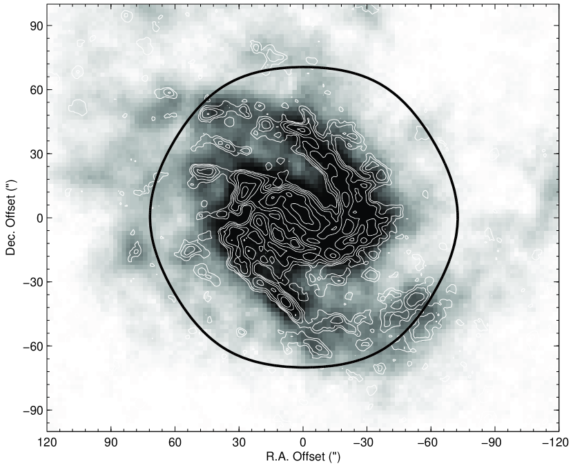
Figure 1.— The contours of velocity integrated CARMA ${\rm CO\ {\it J}=1-0}$ map overlaid on IRAM 30m single dish ${\rm CO\ {\it J}=2-1}$ map. The circle shows that part of the disk where CARMA interferometer observation is the most sensitive. Within this region the agreement between the two maps is excellent. The contours are in logarithmic scale with the levels at 2, 2.9, 4.3, 6.3, 9.3, 13.6 and 20 $\rm Jy~{}Beam^{-1}\ km\ sec^{-1}$. The peak flux of CARMA map is 26 $\rm Jy~{}Beam^{-1}\ km\ sec^{-1}$.

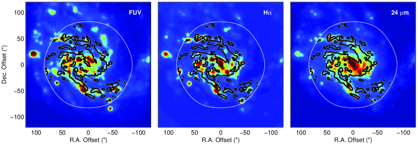
Figure 2.— Multi-wavelength maps of NGC 4254. The panels show FUV, $\rm H\alpha$, and MIR 24 $\mu$m emission maps from left to right. The images are shown in logarithmic scale. The black contours represent the layout of ${\rm CO\ {\it J}=1-0}$ map used in this study. The contours are in linear scale with the levels at 3 and 12 $\rm Jy~{}Beam^{-1}\ km\ sec^{-1}$. The figure shows a striking similarity between the distributions of hot dust traced by the MIR map and the cold molecular gas traced by ${\rm CO\ {\it J}=1-0}$ in both upper an lower arm of the galaxy.

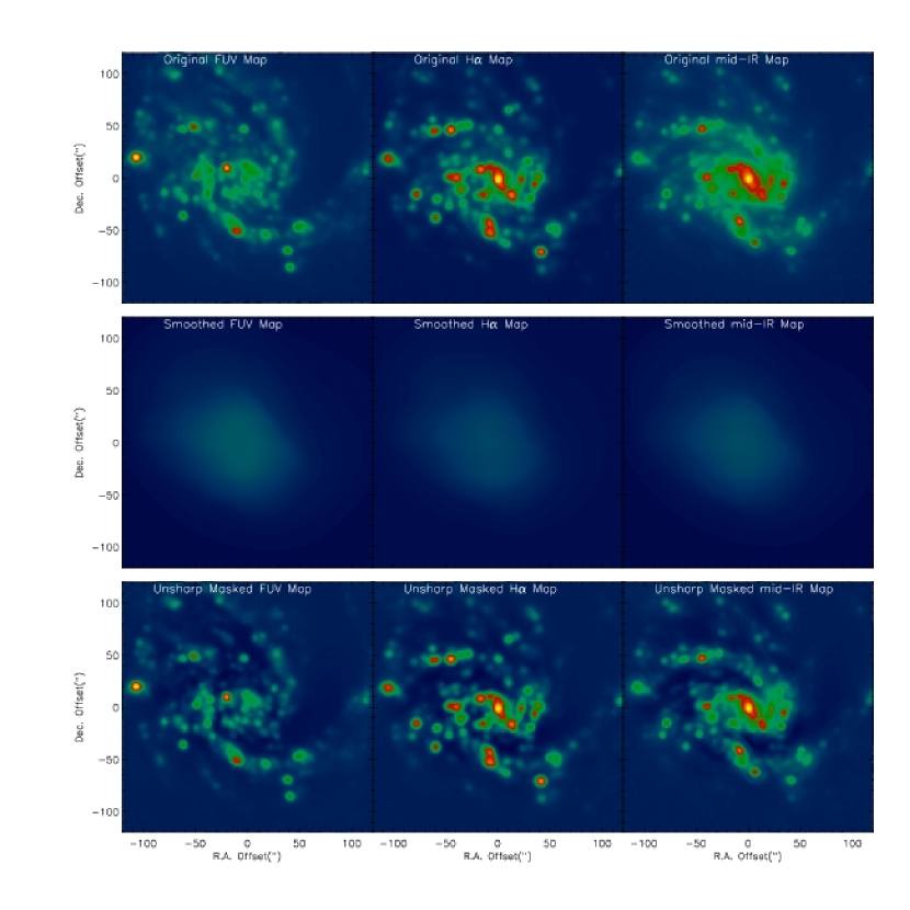
Figure 3.— Two-dimensional unsharp masking. The top panels show the original FUV, $\rm H\alpha$ and MIR 24 $\mu$m emission maps from left to right. The middle panels show the corresponding smoothed images where the smoothing is performed by a 2D box kernel with the kernel size of 105″. The smoothed images are subtracted from the corresponding un-smoothed original images to produce unsharp masked maps (bottom panels).

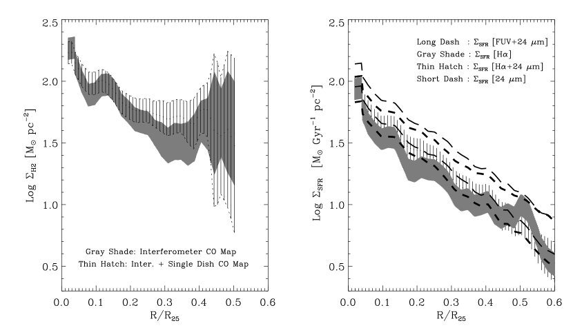
Figure 4.— Azimuthally averaged radial profiles of surface density maps shown at $1\sigma$ up and below the mean trend at each radial point. Left Panel: The radial distribution of molecular gas surface density is shown for the most sensitive CARMA interferometer ${\rm CO\ {\it J}=1-0}$ observation. The profiles derived from interferometer data alone as well as combining interferometer and single dish data are shown by gray shade and thin hatch, respectively. Right Panel: The radial profiles derived from $\Sigma_{{\rm FUV}+24\,\hbox{$\mu$m}}$, $\Sigma_{{\rm H\alpha}}$, $\Sigma_{{\rm H\alpha}+24\,\hbox{$\mu$m}}$, and $\Sigma_{24\,\hbox{$\mu$m}}$ maps are shown by long dashed line, thick hatched region, thin hatched region, and short dashed line, respectively.

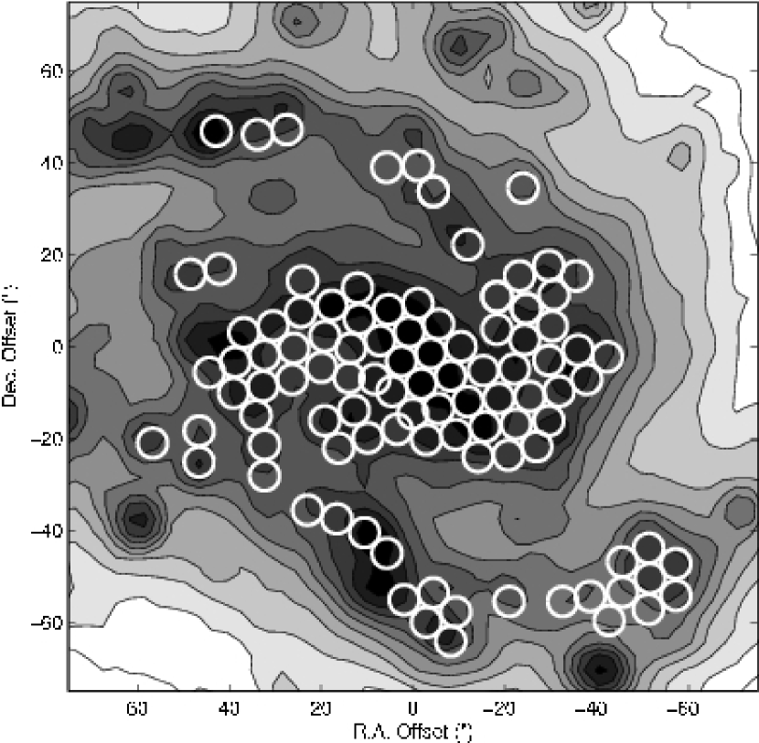
Figure 5.— The $\Sigma_{{\rm H\alpha}+24\,\hbox{$\mu$m}}$ map with the 6″ (500 pc) diameter apertures overlaid. The total number of such apertures is 102.

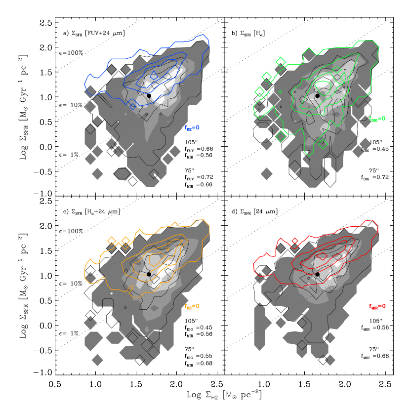
Figure 6.— Pixel-by-pixel analysis all four SFR tracers. The figure shows the molecular gas-SFR surface density relations at two representative filter scales, 105″ (filled contours) and 180″ (black unfilled contours) as well as the case of no filtering, i.e., when ${f_{\rm DE}}$=0 (colored unfilled contours). At any smoothing scale the amount of DE varies in the maps as shown at the bottom right in each panel (see also Table 2). The gray scale represent the two dimensional histogram of the frequency of points, and the contours are placed at 90%, 75%, 50%, and 25% of the maximum frequency. The diagonal dotted lines represent constant SFE ($\rm\epsilon$) where $\rm{\epsilon}\sim$100%, 10%, and 1% correspond to gas depletion time scale of 0.1, 1.0, and 10 Gyr. The filled circle represents the disk averaged estimate within the $\rm R_{25}$. The correlation strength varies among the maps. For a given SFR map, it depends on the degree of unsharp masking. The Pearson correlation coefficients at 105″ and 180″ are $\rm r\sim 0.4-0.55$ (weak correlation) and $\sim 0.55-0.7$ (strong correlation), respectively, indicating how the subtraction of DE influence the correlation between the points. A comparison of the distributions of points shown by filled and unfilled contours clearly shows that the subtraction of DE affects the low surface density regions.

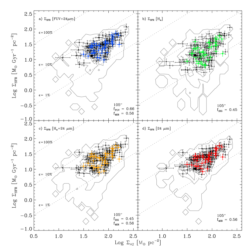
Figure 7.— Aperture analysis for all SFR tracers for the selected apertures as shown in Fig. 5. The faint lines correspond to the contours of pixel distributions at 105″ filter scale (shown as filled contours in Fig. 6). The diagonal dotted lines present constant efficiencies as in Fig. 6.

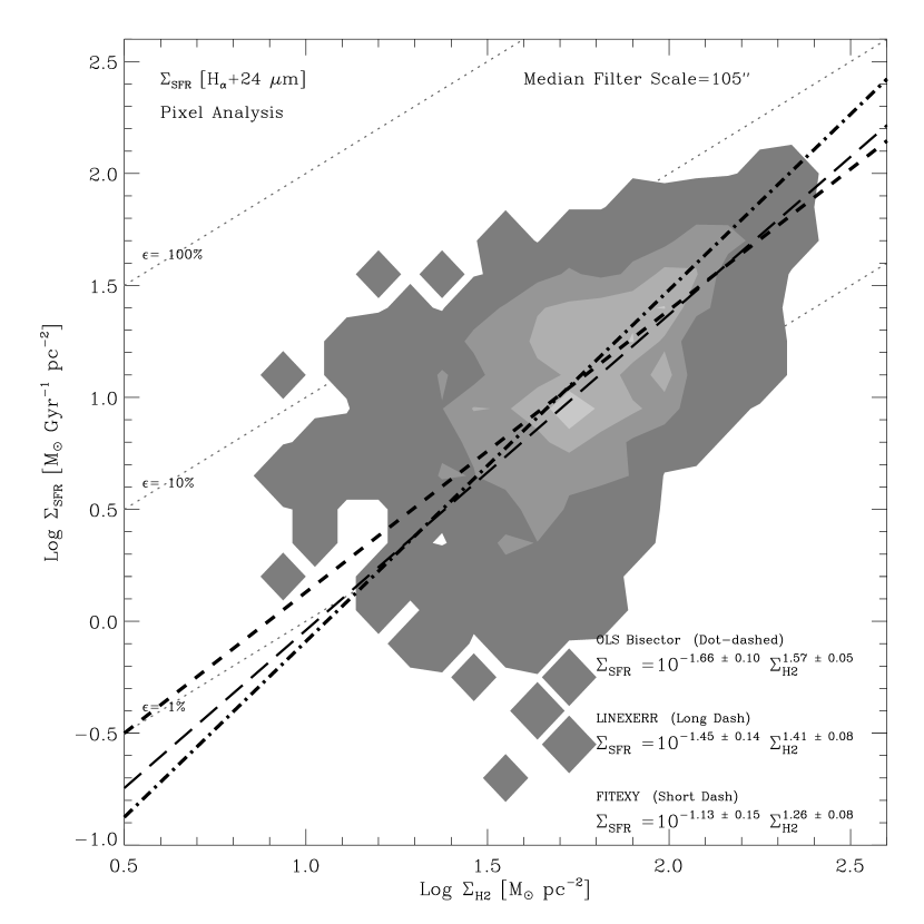
Figure 8.— Measurements provided by bivariate regression methods for $\Sigma_{{\rm H\alpha}+24\,\hbox{$\mu$m}}$ - $\Sigma_{\rm H_{2}}$ relation using pixel-by-pixel sampling. The SFR tracer is subject to unsharp making with a smoothing scale of 105″ which results in ${f_{\rm DIG}}$=0.45 and ${f_{\rm MIR}}$=0.56. The gray scale represent the two dimensional histogram of the frequency of points, and the contours are placed at 90%, 75%, 50%, and 25% of the maximum frequency. For this particular distribution of points, the FITEXY provides the shallowest slope ($\hbox{$\rm N_{mol}$}\sim 1.3$ short dash line) The OLS bisector ($\hbox{$\rm N_{mol}$}\sim 1.6$ dashed-dot line) and the LINEXERR ($\hbox{$\rm N_{mol}$}\sim 1.4$ long dash line) methods, on the other hand, provide steeper estimates. The estimated slope, zero point, and formal error provided by individual fit are shown at the lower right corner. The intrinsic scatter provided by FITEXY, OLS bisector, and LINEXERR methods are $\mbox{$\rm\sigma_{i}$}\sim 0.4$ 0.3, and 0.3 dex, respectively. The vertical and horizontal axes range from $\sim 0.1-114\ \mbox{$\rm M_{\odot}\ Gyr^{-1}\ pc^{-2}$}$ and $\sim 10-245\ \hbox{$\rm M_{\odot}\ pc^{-2}$}$, respectively.

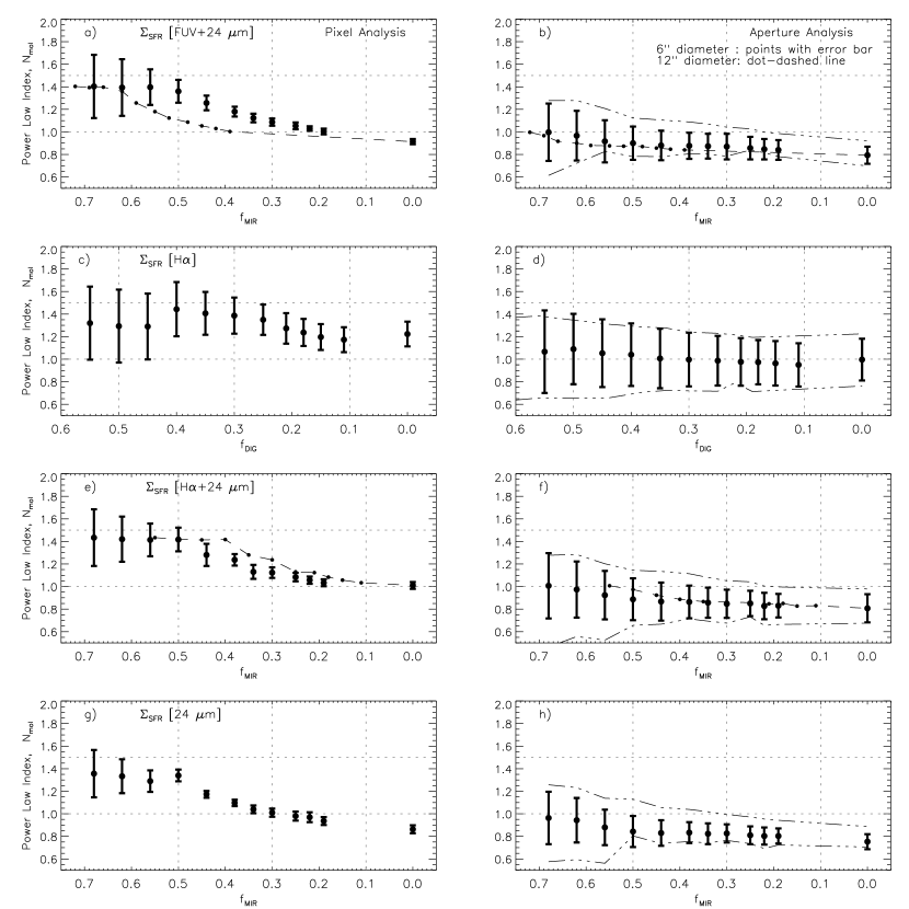
Figure 9.— Dependence of the power law index ($\rm N_{mol}$) of the molecular gas SF law on various diffuse fractions. The figure summarizes results for both pixel (left panels) and aperture (right panels) samplings. Results from $6\arcsec\sim 500$ pc (points) and $12\arcsec\sim 1$ kpc (dashed-dot line) diameter aperture samplings are shown in the right panels. The methodological mean ($\rm{\bar{N}_{mol,fit}}$) and dispersion ($\rm\sigma_{mol,fit}$) from three measurements are shown, respectively, by gray filled circles and vertical lines. The black points connected by dashed lines in panels a and b (e and f) represent the locus of $\rm{\bar{N}_{mol,fit}}$ at ${f_{\rm FUV}}$(${f_{\rm DIG}}$). The horizontal dotted lines represent $\hbox{$\rm N_{mol}$}=1$ and $\hbox{$\rm N_{mol}$}=1.5$. The vertical dotted lines demarcate the regions where the DE is assumed to be (from left to right) the dominant, significant, sub-dominant, and negligible component of the total disk emission. Each point along the horizontal axis has 15% uncertainty (see appendix F for details).

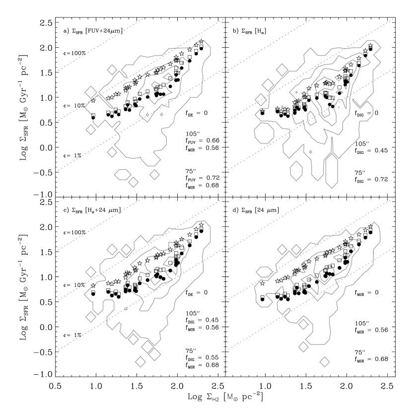
Figure 10.— Azimuthally averaged radial profile analysis all four SFR tracers. Figure shows the radial relations at the dominant (filled circle), significant (open square) and negligible ($\hbox{${f_{\rm DE}}$}=0$) diffuse fractions. The faint lines correspond to the contours of pixel distributions at 105″ filter scale (shown as filled contours in Fig. 6). The diagonal dotted lines represent constant efficiencies as in Fig. 6. The bin size is 500 pc. The absence of an extended tail along the vertical axis at the low surface density regions, irrespective of the subtraction of the amount of diffuse fractions, indicates that azimuthally averaged radial profile systematically sample the high SFR surface density regions compared to pixel sampling. See Table 7 for the derived fitted parameters for all SFR tracer maps at these three diffuse fractions.

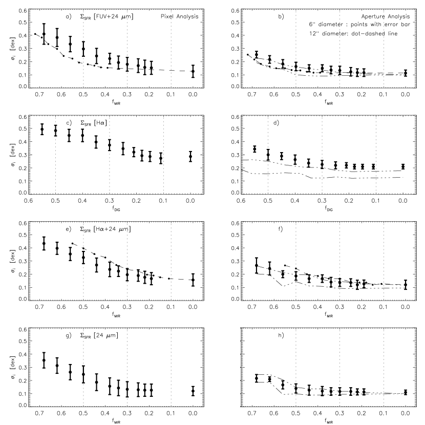
Figure 11.— The intrinsic scatter ($\rm\sigma_{i}$) in the gas-SFR surface density relations at various diffuse fractions for pixel (left panels) and aperture (right panels) samplings. Results from $6\arcsec\sim 500$ pc (points) and $12\arcsec\sim 1$ kpc (dashed-dot line) diameter aperture samplings are shown in the right panels. Figure shows the methodological mean of the observed scatter ($\rm{\bar{\sigma}}_{i,fit}$; “mean dispersion”)by filled circle and the dispersion in the observed scatter (“dispersion of dispersion”) from linear regression methods by vertical solid lines. Figure highlights that the estimate of intrinsic scatter depends on the choice of the SFR tracer as well as on the treatment of DE. For example, the scatter is systematically larger in the $\Sigma_{\rm H_{2}}$- $\Sigma_{{\rm H\alpha}}$ relation (methodological dispersion, $\mbox{$\rm{\bar{\sigma}}_{i,fit}$}\sim 0.3-0.6$ dex). The scatter becomes smaller for larger aperture (dashed-dot line in the right panel) because of the reduction in the sampled points. The vertical lines have similar meanings as in Fig. 9. Each point along the horizontal axis has 15% uncertainty (see appendix F for details).

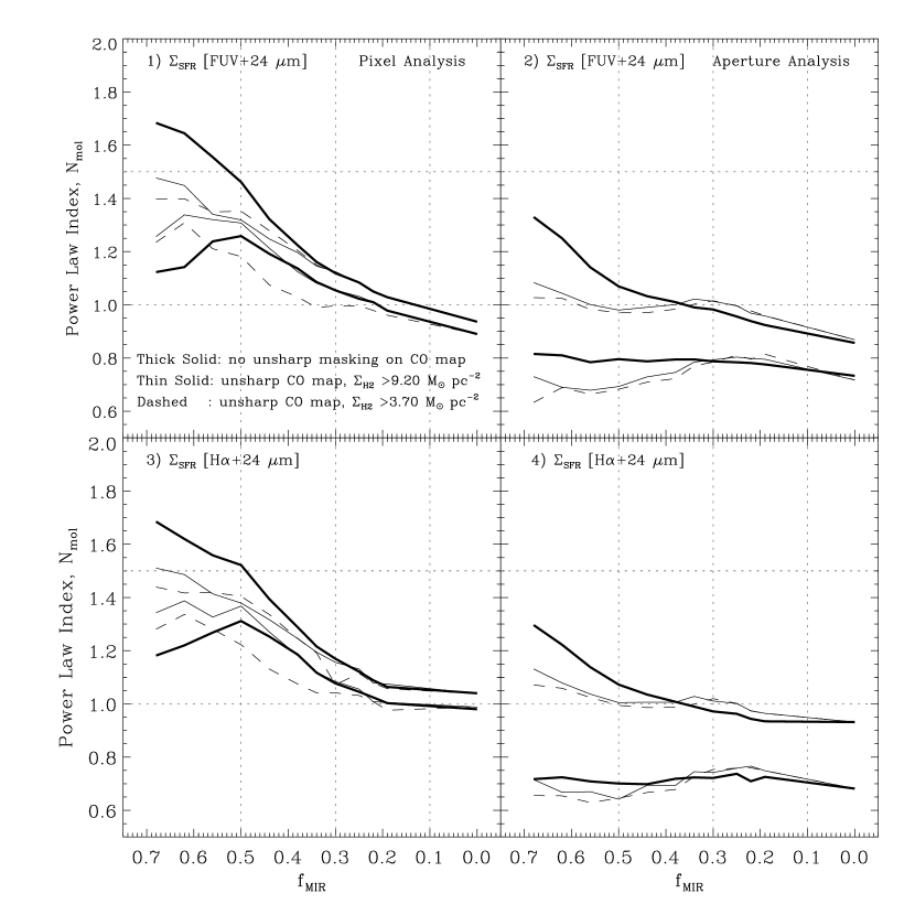
Figure 12.— Dependence of the power law index ($\rm N_{mol}$) of molecular gas SF law when both SFR tracer and ${\rm CO\ {\it J}=1-0}$ map are subject to unsharp masking. The dashed and thin solid lines, respectively, show the methodological dispersions when the selection threshold for the data in the $\Sigma_{\rm H_{2}}$ unsharp-masked map is placed at 1$\sigma$ (3.7 $\rm M_{\odot}\ pc^{-2}$) and 2.5$\sigma$ (9.2 $\rm M_{\odot}\ pc^{-2}$). The thick solid line illustrates the case when only the SFR tracers are subject to masking. Presentation style is similar to Fig. 9.

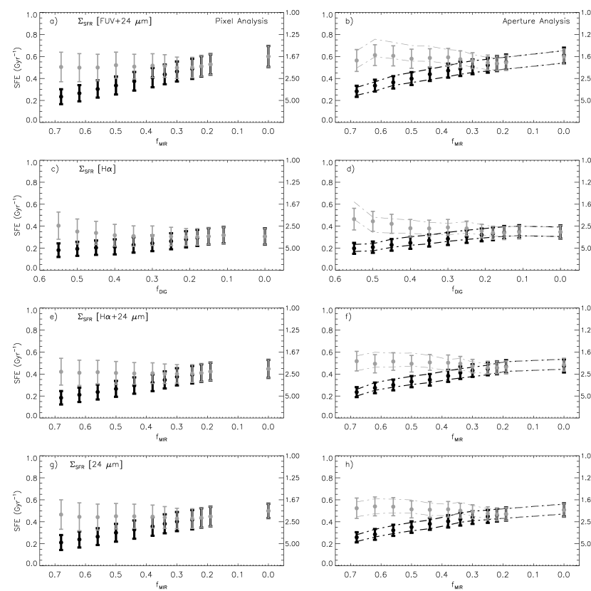
Figure 13.— Disk averaged SFE (Gyr^-1) and the depletion timescale, $\tau_{dep}$ (Gyr), at various diffuse fractions. The SFE and the $\tau_{dep}$ are shown on the left and right vertical axis, respectively. Results for both (6″ by points and 12″ by dashed-dot line) aperture samplings are shown in the right panels. Parameters estimated from applying unsharp masking to the SFR tracer only, and to both the SFR and the gas maps, are shown in black and gray respectively. For a given SFR tracer, the subtraction of DE introduces $\sim$50% ($\Sigma_{{\rm H\alpha}}$) up to a factor 3 variations in the global SFE. At a given ${f_{\rm DE}}$, the global SFE derived from four tracers are approximately consistent with one another (see Table 3), although $\rm H\alpha$ yields a lower depletion time. The dashed lines added by black points shown in Figs. 9 and 11 have omitted for clarity of presentation. The vertical lines have similar meanings as in Fig. 9.

Table 4Fitted Parameters from Pixel Analysis

Filt.	${f_{\rm DIG}}$		FUV+24 $\mu$m			$\rm H\alpha$			$\rm H\alpha$+24 $\mu$m			24 $\mu$m
($\arcsec$)		Log A	$\rm N_{mol}$	$\rm\sigma_{i}$	Log A	$\rm N_{mol}$	$\rm\sigma_{i}$	Log A	$\rm N_{mol}$	$\rm\sigma_{i}$	Log A	$\rm N_{mol}$	$\rm\sigma_{i}$
		${-1.97\pm 0.11}$	$1.71\pm 0.06$	0.50	${-1.99\pm 0.13}$	$1.67\pm 0.07$	0.54	${-2.04\pm 0.11}$	$1.70\pm 0.06$	0.49	${-1.75\pm 0.10}$	$1.57\pm 0.05$	0.42
75	0.55	${-0.96\pm 0.14}$	$1.15\pm 0.07$	0.37	${-0.83\pm 0.20}$	$1.02\pm 0.11$	0.47	${-1.12\pm 0.17}$	$1.19\pm 0.09$	0.40	${-1.00\pm 0.13}$	$1.15\pm 0.07$	0.33
		${-1.36\pm 0.16}$	$1.35\pm 0.09$	0.36	${-1.29\pm 0.21}$	$1.25\pm 0.11$	0.47	${-1.55\pm 0.18}$	$1.40\pm 0.10$	0.41	${-1.40\pm 0.15}$	$1.35\pm 0.08$	0.31
		${-1.57\pm 0.10}$	$1.57\pm 0.05$	0.40	${-1.79\pm 0.10}$	$1.60\pm 0.05$	0.50	${-1.66\pm 0.09}$	$1.57\pm 0.05$	0.41	${-1.27\pm 0.08}$	$1.38\pm 0.04$	0.33
105	0.45	${-1.06\pm 0.13}$	$1.27\pm 0.07$	0.30	${-0.77\pm 0.16}$	$1.02\pm 0.09$	0.42	${-1.13\pm 0.15}$	$1.26\pm 0.08$	0.32	${-0.95\pm 0.12}$	$1.19\pm 0.06$	0.23
		${-1.26\pm 0.13}$	$1.36\pm 0.07$	0.30	${-1.22\pm 0.18}$	$1.25\pm 0.10$	0.42	${-1.45\pm 0.14}$	$1.41\pm 0.08$	0.33	${-1.19\pm 0.11}$	$1.30\pm 0.06$	0.23
		${-0.50\pm 0.05}$	$1.10\pm 0.03$	0.24	${-1.28\pm 0.07}$	$1.41\pm 0.04$	0.36	${-0.68\pm 0.05}$	$1.15\pm 0.05$	0.25	${-0.34\pm 0.04}$	$0.98\pm 0.02$	0.20
180	0.21	${-0.44\pm 0.09}$	$1.05\pm 0.05$	0.15	${-0.83\pm 0.13}$	$1.15\pm 0.07$	0.30	${-0.57\pm 0.09}$	$1.07\pm 0.05$	0.17	${-0.42\pm 0.07}$	$1.00\pm 0.04$	0.10
		${-0.58\pm 0.08}$	$1.11\pm 0.04$	0.15	${-1.10\pm 0.12}$	$1.27\pm 0.07$	0.30	${-0.74\pm 0.08}$	$1.15\pm 0.04$	0.17	${-0.53\pm 0.07}$	$1.05\pm 0.04$	0.10
		${-0.03\pm 0.04}$	$0.90\pm 0.02$	0.18	${-1.10\pm 0.06}$	$1.33\pm 0.03$	0.33	${-0.36\pm 0.04}$	$1.01\pm 0.02$	0.21	${-0.02\pm 0.04}$	$0.82\pm 0.02$	0.16
–	0.0	${-0.06\pm 0.06}$	$0.90\pm 0.03$	0.10	${-0.74\pm 0.11}$	$1.12\pm 0.06$	0.27	${-0.34\pm 0.07}$	$0.98\pm 0.04$	0.13	${-0.07\pm 0.05}$	$0.86\pm 0.03$	0.10
		${-0.16\pm 0.06}$	$0.94\pm 0.03$	0.10	${-0.97\pm 0.11}$	$1.23\pm 0.06$	0.26	${-0.47\pm 0.07}$	$1.04\pm 0.04$	0.13	${-0.16\pm 0.05}$	$0.90\pm 0.03$	0.10

Note. — The normalization constant, power-law index, and intrinsic scatter of the molecular gas SF law are derived from unsharp masked SFR tracers (i.e., unsharp masking along the vertical axis). The filter scales from the top correspond to the dominant ($\hbox{${f_{\rm DIG}}$}\gtrsim 50\%$), significant ($\hbox{${f_{\rm DIG}}$}\sim 30-50\%$), and sub-dominant ($\hbox{${f_{\rm DIG}}$}\sim 10-30\%$) diffuse fractions. The bottom row shown by the dashed line represents ${f_{\rm DIG}}$=0. At a given filter scale, the three rows under FUV+24$\mu$m provide the measurements of the OLS bisector, FITEXY, and LINEXERR fitting method, respectively. Typical uncertainty in the intrinsic scatter is few percent.

Table 5Fitted Parameters from 6″ Aperture Analysis

Filt.	${f_{\rm DIG}}$		FUV+24 $\mu$m			$\rm H\alpha$			$\rm H\alpha$+24 $\mu$m			24 $\mu$m
($\arcsec$)		Log A	$\rm N_{mol}$	$\rm\sigma_{i}$	Log A	$\rm N_{mol}$	$\rm\sigma_{i}$	Log A	$\rm N_{mol}$	$\rm\sigma_{i}$	Log A	$\rm N_{mol}$	$\rm\sigma_{i}$
		${-0.09\pm 0.17}$	$1.29\pm 0.09$	0.28	${-1.61\pm 0.22}$	$1.49\pm 0.11$	0.37	${-1.27\pm 0.17}$	$1.34\pm 0.08$	0.30	${-1.03\pm 0.16}$	$1.23\pm 0.08$	0.25
75	0.55	${-0.26\pm 0.23}$	$0.84\pm 0.12$	0.25	${-0.40\pm 0.37}$	$0.85\pm 0.20$	033	${-0.30\pm 0.23}$	$0.82\pm 0.12$	0.20	${-0.24\pm 0.23}$	$0.80\pm 0.12$	0.20
		${-0.30\pm 0.26}$	$0.86\pm 0.14$	0.23	${-0.51\pm 0.35}$	$0.90\pm 0.19$	0.33	${-0.39\pm 0.28}$	$0.86\pm 0.15$	0.30	${-0.35\pm 0.24}$	$0.86\pm 0.13$	0.20
		${-0.67\pm 0.14}$	$1.13\pm 0.07$	0.22	${-0.34\pm 0.18}$	$1.40\pm 0.09$	0.32	${-0.84\pm 0.14}$	$1.17\pm 0.07$	0.23	${-0.61\pm 0.13}$	$1.06\pm 0.07$	0.20
105	0.45	${-0.03\pm 0.16}$	$0.78\pm 0.08$	0.16	${-0.33\pm 0.30}$	$0.86\pm 0.16$	0.27	${-0.10\pm 0.21}$	$0.78\pm 0.11$	0.18	${-0.06\pm 0.18}$	$0.77\pm 0.10$	0.16
		${-0.13\pm 0.20}$	$0.84\pm 0.11$	0.17	${-0.42\pm 0.30}$	$0.90\pm 0.16$	0.28	${-0.19\pm 0.22}$	$0.82\pm 0.12$	0.19	${-0.14\pm 0.19}$	$0.81\pm 0.10$	0.14
		${-0.25\pm 0.12}$	$0.99\pm 0.06$	0.17	${-0.87\pm 0.14}$	$1.22\pm 0.07$	0.24	${-0.35\pm 0.11}$	$0.99\pm 0.06$	0.17	${-0.20\pm 0.10}$	$0.92\pm 0.05$	0.15
180	0.21	${+0.12\pm 0.16}$	$0.79\pm 0.08$	0.12	${-0.16\pm 0.20}$	$0.84\pm 0.11$	0.22	${+0.07\pm 0.15}$	$0.76\pm 0.08$	0.12	${+0.06\pm 0.15}$	$0.78\pm 0.08$	0.10
		${-0.04\pm 0.16}$	$0.82\pm 0.08$	0.11	${-0.23\pm 0.23}$	$0.87\pm 0.12$	0.20	${-0.02\pm 0.17}$	$0.79\pm 0.09$	0.12	${-0.05\pm 0.14}$	$0.78\pm 0.07$	0.10
		${-0.03\pm 0.10}$	$0.88\pm 0.05$	0.14	${-0.83\pm 0.15}$	$1.21\pm 0.08$	0.23	${-0.21\pm 0.11}$	$0.95\pm 0.06$	0.16	${+0.03\pm 0.09}$	$0.83\pm 0.05$	0.13
–	0.0	${+0.29\pm 0.12}$	$0.74\pm 0.07$	0.10	${-0.20\pm 0.18}$	$0.88\pm 0.09$	0.20	${+0.16\pm 0.16}$	$0.75\pm 0.08$	0.10	${+0.24\pm 0.13}$	$0.71\pm 0.06$	0.10
		${+0.24\pm 0.14}$	$0.76\pm 0.07$	0.10	${-0.25\pm 0.22}$	$0.90\pm 0.12$	0.20	${-0.08\pm 0.15}$	$0.78\pm 0.08$	0.10	${+0.22\pm 0.12}$	$0.72\pm 0.06$	0.10

Note. — The normalization constant, power-law index, and intrinsic scatter of the molecular gas SF law are derived from unsharp masked SFR tracers (i.e., unsharp masking along the vertical axis). The filter scales from the top correspond to the dominant ($\hbox{${f_{\rm DIG}}$}\gtrsim 50\%$), significant ($\hbox{${f_{\rm DIG}}$}\sim 30-50\%$), and sub-dominant ($\hbox{${f_{\rm DIG}}$}\sim 10-30\%$) diffuse fractions. The bottom row shown by the dashed line represents ${f_{\rm DIG}}$=0. At a given filter scale, the three rows under FUV+24$\mu$m provide the measurements of the OLS bisector, FITEXY, and LINEXERR fitting method, respectively. Typical uncertainty in the intrinsic scatter is few percent.

Table 6Fitted Parameters from 12″ Aperture Analysis

Filt.	${f_{\rm DIG}}$		FUV+24 $\mu$m			$\rm H\alpha$			$\rm H\alpha$+24 $\mu$m			24 $\mu$m
($\arcsec$)		Log A	$\rm N_{mol}$	$\rm\sigma_{i}$	Log A	$\rm N_{mol}$	$\rm\sigma_{i}$	Log A	$\rm N_{mol}$	$\rm\sigma_{i}$	Log A	$\rm N_{mol}$	$\rm\sigma_{i}$
		${-1.20\pm 0.30}$	$1.33\pm 0.15$	0.23	${-1.42\pm 0.33}$	$1.39\pm 0.17$	0.26	${-1.30\pm 0.33}$	$1.34\pm 0.16$	0.26	${-1.22\pm 0.30}$	$1.31\pm 0.15$	0.25
75	0.55	${-0.12\pm 0.44}$	$0.76\pm 0.23$	0.20	${-0.31\pm 0.67}$	$0.81\pm 0.36$	0.20	${-0.05\pm 0.52}$	$0.63\pm 0.28$	0.20	${-0.11\pm 0.50}$	$0.73\pm 0.26$	0.20
		${-0.10\pm 0.50}$	$0.75\pm 0.26$	0.20	${-0.14\pm 0.56}$	$0.73\pm 0.29$	0.25	${+0.04\pm 0.56}$	$0.64\pm 0.30$	0.24	${-0.07\pm 0.49}$	$0.71\pm 0.26$	0.20
		${-0.88\pm 0.27}$	$1.22\pm 0.13$	0.18	${-1.45\pm 0.35}$	$1.44\pm 0.18$	0.25	${-1.01\pm 0.26}$	$1.25\pm 0.13$	0.20	${-0.84\pm 0.25}$	$1.17\pm 0.12$	0.21
105	0.45	${-0.39\pm 0.84}$	$0.99\pm 0.42$	0.15	${-0.21\pm 0.85}$	$0.82\pm 0.43$	0.15	${+0.25\pm 0.73}$	$0.62\pm 0.37$	0.10	${+0.30\pm 0.42}$	$0.61\pm 0.21$	0.10
		${-0.15\pm 0.39}$	$0.84\pm 0.21$	0.15	${-0.22\pm 0.56}$	$0.80\pm 0.29$	0.23	${-0.02\pm 0.44}$	$0.72\pm 0.23$	0.18	${-0.09\pm 0.37}$	$0.77\pm 0.20$	0.14
		${-0.41\pm 0.21}$	$1.06\pm 0.11$	0.12	${-1.01\pm 0.25}$	$1.28\pm 0.13$	0.20	${-0.54\pm 0.21}$	$1.08\pm 0.11$	0.15	${-0.39\pm 0.21}$	$1.01\pm 0.10$	0.12
180	0.21	${-0.03\pm 0.22}$	$0.82\pm 0.12$	0.10	${-0.17\pm 0.44}$	$0.83\pm 0.23$	0.12	${-0.09\pm 0.27}$	$0.75\pm 0.14$	0.10	${-0.07\pm 0.25}$	$0.84\pm 0.14$	0.10
		${-0.05\pm 0.29}$	$0.86\pm 0.15$	0.10	${-0.16\pm 0.42}$	$0.83\pm 0.22$	0.17	${-0.06\pm 0.32}$	$0.76\pm 0.17$	0.11	${+0.02\pm 0.27}$	$0.79\pm 0.14$	0.10
		${-0.09\pm 0.18}$	$0.93\pm 0.09$	0.10	${-0.94\pm 0.26}$	$1.26\pm 0.13$	0.18	${-0.34\pm 0.20}$	$1.00\pm 0.10$	0.12	${-0.11\pm 0.18}$	$0.90\pm 0.01$	0.10
–	0.0	${-0.31\pm 0.31}$	$0.71\pm 0.17$	0.10	${-0.16\pm 0.32}$	$0.85\pm 0.17$	0.13	${-0.19\pm 0.30}$	$0.72\pm 0.16$	0.10	${-0.15\pm 0.15}$	$0.76\pm 0.08$	0.10
		${+0.17\pm 0.25}$	$0.79\pm 0.13$	0.10	${-0.20\pm 0.39}$	$0.87\pm 0.20$	0.15	${-0.12\pm 0.28}$	$0.76\pm 0.15$	0.10	${+0.21\pm 0.24}$	$0.73\pm 0.13$	0.10

Note. — The normalization constant, power-law index, and intrinsic scatter of the molecular gas SF law are derived from unsharp masked SFR tracers (i.e., unsharp masking along the vertical axis). The filter scales from the top correspond to the dominant ($\hbox{${f_{\rm DIG}}$}\gtrsim 50\%$), significant ($\hbox{${f_{\rm DIG}}$}\sim 30-50\%$), and sub-dominant ($\hbox{${f_{\rm DIG}}$}\sim 10-30\%$) diffuse fractions. The bottom row shown by the dashed line represents ${f_{\rm DIG}}$=0. At a given filter scale, the three rows under FUV+24$\mu$m provide the measurements of the OLS bisector, FITEXY, and LINEXERR fitting method, respectively. Typical uncertainty in the intrinsic scatter is few percent.

Table 7Fitted Parameters from Azimuthally Averaged Radial Profile Analysis

Filt.	${f_{\rm DIG}}$	FUV+24 $\mu$m		$\rm H\alpha$		$\rm H\alpha$+24 $\mu$m		24 $\mu$m
($\arcsec$)		Log A	$\rm N_{mol}$	Log A	$\rm N_{mol}$	Log A	$\rm N_{mol}$	Log A	$\rm N_{mol}$
75	0.55	${-0.82\pm 0.11}$	$1.13\pm 0.07$	${-0.81\pm 0.15}$	$1.09\pm 0.09$	${-0.79\pm 0.13}$	$1.07\pm 0.08$	${-0.94\pm 0.11}$	$1.16\pm 0.06$
105	0.45	${-0.78\pm 0.08}$	$1.17\pm 0.05$	${-0.78\pm 0.12}$	$1.11\pm 0.07$	${-0.76\pm 0.10}$	$1.11\pm 0.06$	${-0.87\pm 0.07}$	$1.18\pm 0.04$
180	0.21	${-0.53\pm 0.04}$	$1.12\pm 0.02$	${-0.63\pm 0.08}$	$1.09\pm 0.05$	${-0.55\pm 0.05}$	$1.08\pm 0.03$	${-0.57\pm 0.03}$	$1.10\pm 0.02$
–	0.0	${-0.16\pm 0.03}$	$0.98\pm 0.02$	${-0.64\pm 0.06}$	$1.12\pm 0.04$	${-0.37\pm 0.04}$	$1.02\pm 0.02$	${-0.20\pm 0.02}$	$0.95\pm 0.01$
75	0.55	${-0.16\pm 0.03}$	$0.98\pm 0.02$	${-0.64\pm 0.06}$	$1.12\pm 0.04$	${-0.37\pm 0.04}$	$1.02\pm 0.02$	${-0.20\pm 0.02}$	$0.95\pm 0.01$
105	0.45	${-0.35\pm 0.06}$	$1.07\pm 0.04$	${-0.38\pm 0.08}$	$1.04\pm 0.05$	${-0.35\pm 0.06}$	$1.02\pm 0.04$	${-0.45\pm 0.05}$	$1.09\pm 0.03$
180	0.21	${-0.20\pm 0.10}$	$1.08\pm 0.06$	${-0.33\pm 0.08}$	$1.07\pm 0.05$	${-0.24\pm 0.08}$	$1.05\pm 0.06$	${-0.24\pm 0.10}$	$1.06\pm 0.04$
–	0.0	${-0.44\pm 0.08}$	$1.12\pm 0.04$	${-0.48\pm 0.08}$	$1.08\pm 0.05$	${-0.46\pm 0.06}$	$1.08\pm 0.04$	${-0.53\pm 0.07}$	$1.14\pm 0.04$

Note. — Top: parameters in the top four rows are derived from unsharp masked SFR tracer maps. Bottom: parameters in the bottom four rows are derived when both molecular gas and SFR maps are subject to unsharp masking. The intrinsic scatter $\rm\sigma_{i}$ is 0 in radial profile analysis and hence the parameters are obtained from the OLS bisector method. The filter scales from the top correspond to the dominant ($\hbox{${f_{\rm DIG}}$}\gtrsim 50\%$), significant ($\hbox{${f_{\rm DIG}}$}\sim 30-50\%$), and sub-dominant (($\hbox{${f_{\rm DIG}}$}\sim 10-30\%$) diffuse fractions. The bottom row shown by the dashed line represents ${f_{\rm DIG}}$=0.

Appendix A NGC 4254

The optical structure of NGC 4254 shows a one-armed appearance ($\rm m=1$ mode), unlike most grand-design spirals where symmetric modes are prominent. This unusual morphology has made it the target of several observational and numerical studies (Phookun et al. 1993; Chemin et al. 2006; Sofue et al. 2003). Various explanations for its asymmetry have been put forth including the superposition of spiral modes induced by global gravitational instability (Iye et al. 1982), the asymmetric accretion of gas onto the disk (Phookun et al. 1993; Bournaud et al. 2005), ram pressure stripping (Sofue et al. 2003; Kantharia et al. 2008), a close high-speed encounter plus ram pressure (Vollmer et al. 2005), a high-speed encounter only (Duc & Bournaud 2008), and harassment while entering Virgo (Haynes et al. 2007). On the other hand, detailed photometric studies of NGC 4254 show that it is photometrically similar to other Sc type spirals, and it has no close companion (Phookun et al. 1993).

NGC 4254 has a flat rotation curve with $v_{rot}\sim 150$ km  sec^-1 up to 200″ ($\sim 16$ kpc) from its center (Guhathakurta et al. 1988). Apart from its morphological peculiarity, it does not show any anomaly in its properties. For example, the distribution of SF through out the disk based on $\rm H\alpha$ emission has been classified as normal (Koopman & Kenney 2004). Its molecular gas fraction in the disk is similar to field galaxies, suggesting that it is entering Virgo for the first time and external agents (such as ram pressure) have not yet been effective at striping its gas, despite its morphology (Nakasihsi et al. 2006). NGC 4254 is a metal rich galaxy with a median $\rm 12+\log[O/H]\sim 9.0$ across the disk (Vila-Costas & Edmunds 1992; Zaritsky et al. 1994).

Appendix B SFR Surface Density Maps

We construct four different SFR maps from combining FUV and MIR maps (Leroy et al. 2008), optical $\rm H\alpha$ emission map (Kennicutt et al. 2007; Prescott et al. 2007), optical $\rm H\alpha$ emission and MIR maps (Calzetti et al. 2007), and MIR map (Calzetti et al. 2007). The details of the construction of these SFR tracers can be found in the references. These different SFR tracers probe different time scales and hence the SF history of any particular galaxy. For example, the $\rm H\alpha$ emission traces gas ionized by massive ($\rm M>10\ \hbox{$\rm M_{\odot}$ }$) stars over a timescale of $<20$ Myr. The FUV luminosity corresponds relatively older ($<100$ Myr), less massive ($\rm M\gtrsim 5\ \hbox{$\rm M_{\odot}$ }$) stellar populations. The MIR 24 $\mu$m emission mostly traces re-processed radiation of newborn (few Myr) OB stellar associations embedded inside the parent molecular clouds. Although star clusters break from their parent clouds in less than 1 Myr, they remain associated with it for a much longer time scale, $t\sim 10-30$ Myr. Thus this is the time scale associated with the MIR 24 $\mu$m emission as a tracer. However, if there is significant heating of the small dust grains by late B and A stars, the time scales associated with 24 $\mu$m emission may be as long as $\sim 100$ Myr. For composite SFR tracer such as FUV + 24 $\mu$m or $\rm H\alpha$ + 24 $\mu$m  while the MIR emission traces the dust-obscured fraction of the SF, and the un-obscured SF can be traced either by FUV continuum or optical nebular emission.

Each pixel in the FUV, $\rm H\alpha$, and 24 $\mu$m emission maps has some uncertainties coming from observation and data processing. These errors propagate to the uncertainties in the surface density maps. For example, uncertainties in the flux calibration, the stellar continuum subtraction, and the background subtraction contribute to the total error budget of $\rm H\alpha$. We assume 10% uncertainty for each of these components and construct $\rm H\alpha$ error map $\rm\sigma_{H\alpha}$ by adding these terms quadratically. A flat 10% uncertainty in stellar continuum subtraction for the entire galaxy disk is probably unrealistic because stellar emission dominates in the galaxy center. Therefore, it will have higher contribution at the high surface brightness regions. We take this limit on ad hoc basis. The assumed fraction in the continuum subtraction may a lower limit since it varies along the galaxy disk contributing as much as 30% to $\rm I_{H\alpha}$ flux uncertainty (Koopman et al. 2001). Finally, there is a considerable (calibration) uncertainty in $\rm H\alpha$ to SFR conversion (Calzetti et al. 2007). We take all these factors into consideration when constructing the SFR error map ($\rm\sigma_{H\alpha}$) from the H$\alpha$ image. The FUV and mid-IR error maps ($\rm\sigma_{FUV}$ and $\rm\sigma_{MIR}$) are constructed in a similar manner but without the contribution from the stellar continuum. The error in the composite SFR maps (FUV + 24 $\mu$m or $\rm H\alpha$ + 24 $\mu$m) are constructed by combining the appropriate terms from the respective images.

Appendix C Molecular Gas Surface Density Map

A conversion factor ($\rm X_{CO}$) is frequently used to determine the distribution of molecular hydrogen (${\rm H_{2}}$) from the ${\rm CO\ {\it J}=1-0}$ images. In this study, we use $\hbox{$\rm X_{CO}$}=2.0\times 10^{20}$ to be consistent with several other current studies (Wong & Blitz 2002; Komugi et al. 2005; Gardan et al. 2007; Bigiel et al. 2008; Leroy et al. 2008). The choice of the calibration factor linearly scales the estimated gas densities. It is worthwhile asking how accurate is the assumption of a single conversion factor. Although the CO-to-H₂ appears to be approximately constant for resolved GMCs (Bolatto et al. 2008), on the hundreds of parsecs scales sampled in this study it may vary across the disk, especially in the low density low metallicity regions (e.g., Garcia-Burillo et al. 1993). We adopt a constant $\rm X_{CO}$ for simplicity and consistency with most recent studies (Wong & Blitz 2002; Komugi et al. 2005; Gardan et al. 2007; Bigiel et al. 2008; Leroy et al. 2008). Furthermore, we expect the effects of a varying conversion factor to be most important in the outer portions of the disk, which are beyond the central region sampled by this study. The ${\rm H_{2}}$ surface densities are multiplied by a factor of 1.40 to account for the mass contribution of helium and are expressed in units of $\rm M_{\odot}\ pc^{-2}$.

To obtain the integrated (interferometer + single) CO map, first, the CARMA cube was de-convolved using the implementation of the CLEAN algorithm in the MIRIAD task mossdi and the velocity channels (2.6 km  sec^-1) in the IRAM cube has been re-binned to have the same velocity resolution (10 km  sec^-1) of the CARMA cube. The MIRIAD task immerge was then used to combine the CARMA and the IRAM cube in the image plane (e.g., Stanimirović et al. 1999). The integrated intensity map was created by convolving each plane of the original data-cube with a 15″ Gaussian to degrade its resolution, selecting regions in each velocity plane where the signal is larger than 2.5$\sigma$, and using these regions as masks on the original cube to compute an integrated intensity. The corresponding error map was computed by considering the $1\sigma$ rms value of 22 m$\rm Jy~{}Beam^{-1}\ km\ sec^{-1}$ for each plane and multiplying by the square root of the number of planes that make up each integrated intensity point. Although the RMS in each plane is approximately constant within the field-of-view of the mosaic, the noise in the integrated intensity map is a function of position because of the change in line width of the CO emission.

Appendix D Data Sampling

Existing studies of spatially resolved SF law in galaxies use three different data sampling methodologies. These are: azimuthally averaged radial profile (Kennicutt 1989; Martin & Kennicutt 2001; Wong & Blitz 2002; Boissier et al. 2003; Heyer et al. 2004; Schuster et al. 2007; Bigiel et al. 2008); aperture analysis encompassing the star forming regions and centering on $\rm H\alpha$ and MIR 24 $\mu$m emission peaks (Kennicutt et al. 2007; Blanc et al. 2009); and finally, pixel-by-pixel analysis (Bigiel et al. 2008; Leroy et al. 2008). To understand the methodological impact on the determination of the local SF law we have incorporated all three methods in our study since each of these methodologies has strengths and weaknesses.

Pixel analysis probes the gas-SFR density relation at the smallest spatial resolution. Aperture averages, on the other hand, provide information relevant to ensemble averages of representative regions. Azimuthally averaged radial profiles, in general, provide estimates over much larger scales. This method of sampling produces overall radial trends suppressing local variations. Radial profiles, by construction, are less susceptible to angular resolution. Although the first sampling probes the smallest spatial scales in the map, it is heavily dominated by its low surface brightness regions. The latter two samplings, by construction, probe only the high surface brightness regions where our signal-to-noise is best and DE in both the SFR and the molecular gas tracers is likely to be a minor contaminant.

In our pixel analysis, we consider regions of the galaxy where both $\Sigma_{\rm SFR}$ and $\Sigma_{\rm H_{2}}$ are higher than $2.5\sigma$. All images are resolution-matched to 6″, and re-sampled at the Nyquist rate ($3\arcsec\times 3\arcsec$ pixels). For the aperture analysis we lay down a total of 102 circular apertures 6″ (500 pc) in diameter, in regions of high surface density, mostly following the spiral arms (see Fig. 5). These apertures are approximately independent, with only a small fraction (5%) of overlap. We also consider 34 circular apertures 12″ (1 kpc) in diameter with a similar overlapping fraction. It should be stressed here that sampling the same region in all four SFR surface density maps simultaneously determines the total number of apertures. The aperture centers for both small and large radii were chosen independently. For any $\Sigma_{\rm SFR}$ map all the apertures combined cover approximately $\approx 45\%$ of the total area covered by all the pixels above $2.5\sigma$ limit. Because of the nature of the selection method the aperture samplings contain $\sim 65\%$ of the total emission when compared pixel sampling.

Appendix E Statistical Methodology and Fitting Procedures

The SF law, as expressed by Eq. 1, is a power law relationship between the SFR surface density and the gas surface density. The outcome of any regression analysis, with the object of finding $\rm A$ and $\rm N$, depends on the treatment of the data and its measurement errors, and on the intrinsic scatter of the observables. The intrinsic scatter reflects the variations of local physical properties of star-forming regions (for example, evolutionary stages, stellar populations, metallicity, obscuration, etc). The measurement errors, on the other hand, depend entirely upon the observations and the subsequent data reduction. The factors that contribute to the measurement errors include flux calibration, continuum subtraction, and background subtraction.

The linear regression methods can be divided into two broad classes depending on whether the intrinsic scatter or the measurement error dominate. When seeking a linear relationship between two variables in a data set where both of them have small measurement errors but substantial yet unknown intrinsic scatter, the ordinary least square (OLS) bisector method provides one the best solutions, (Isobe et al. 1990; Feigelson & Babu 1992).

When both the dependent and the independent variables are subject to measurement errors and intrinsic scatter of comparable magnitude, the regression analysis becomes more complex. Several bivariate regression methods have been developed to deal with astronomical problems but each method has its own advantages and disadvantages (see Feigelson & Babu 1992 for a detailed account). The most widely used bivariate regression analysis is based on the least squares technique (FITEXY; Press et al.1992 and references therein). Akritas & Bershady (1996) extended the OLS bisector method incorporating measurement error and the intrinsic scatter. This estimator is known as the bivariate correlated error and scatter (BCES) estimator. Kelly (2007) developed a bivariate estimator based on Bayesian statistics (LINEXERR).

The FITEXY and LINEXERR estimators differ in the underlying assumption of the nature of the true relationship between independent and dependent variables. Both the BCES and LINEXERR estimators assume that the data points are scattered around the true linear relationship. The FITEXY, on the other hand, assumes that there is no intrinsic scatter and the true points lie exactly on a straight line, providing a solution for data showing a perfect correlation. While the BCES and LINEXERR estimators incorporate the correlated measurement error, FITEXY does not account for it. Correlated error arises when the dependent and the independent variables both are subjected to the same uncertainty. For example, surface densities are defined as the ratio of the total mass to the de-projected area of the disk. An uncertainty in the inclination measurement leads to a correlated measurement error in the surface density of gas and SFR. The covariance term broadens the actual distribution of data points and thus provides a flatter relationship if unaccounted for (Akritas & Bershady 1996).

In this study we have used the OLS bisector, FITEXY, and LINEXERR estimators. We note here that while the OLS bisector method will guard our analysis against possible flaw in constructing measurement error maps, the other two methods will be required for a complete analysis of data. Our experience shows that the BCES bisector method is highly sensitive to the measurement error resulting in unstable slope estimates compared to the three other methods mentioned above. We do not use this estimator in our analysis.

We construct surface density measurement error maps as mentioned in section $\S$2. The covariant term for each pixel is calculated from the error map. The intrinsic scatter is directly provided by the LINEXERR estimator. For the OLS bisector and FITEXY estimators we estimate it using the best fit line. To include scatter in the FITEXY estimator we iteratively adjust the error along the Y-axis iteratively until we achieve a reduced chi-squared $\sim 1$. For this estimator, the total dispersion along the y-axis is $\rm\sigma_{y}^{2}=\sigma_{m}^{2}+\sigma_{i}^{2}$. The adjustment is made for $\rm\sigma_{i}$ which is a measure of the intrinsic dispersion in the gas-SFR surface density relation, while $\sigma_{m}$ is the measurement uncertainty obtained from error propagation. The formal error in each parameter quoted in this paper comes from the bootstrap sampling of 1000 realizations of the data points.

Appendix F Unsharp Masking

We use unsharp masking to model and remove the local variations of DE from the maps. The choice of the size of the median filter kernel plays a vital role in selecting the amount of diffuse component in the total disk emission. As mentioned earlier, we explore a number of filter sizes in each SFR tracer, carrying out our analysis for each case (see Table 2). We should stress here that our intention is to use the simplest model for a reliable estimate of the diffuse fraction in the disk of NGC 4254 which can be used with a reasonable confidence to explore the main goal of this study.

For a filter size of 75″ the fraction of the total emission contained in the smooth $\rm H\alpha$ map is $\hbox{${f_{\rm DIG}}$}\sim 60\%$, on the acceptable high-end of the DIG fractions observed in other galaxies (Kennicutt et al. 1995; Ferguson et al. 1996). Thus, DE in $\rm H\alpha$ is likely overestimated for kernel sizes below 75″ (corresponding to physical scales $\sim 6$ kpc). Using smaller kernels for unsharp masking results in over-subtracted maps containing undesirable artifacts (many negative pixels and increased scatter). The upper end of acceptable kernel sizes is determined by the image size. We set it roughly to two-third the image size, corresponding to $210\arcsec$ or a physical length of $\sim 13$ kpc. With this scale we obtain $\hbox{${f_{\rm DIG}}$}\sim 15\%$ which is approximately the ${f_{\rm DIG}}$ observed in the Galaxy (Reynolds 1991). Similar kernel sizes are also explored in the FUV and 24 $\mu$m maps. As expected, the diffuse fractions in the FUV, $\rm H\alpha$, and 24 $\mu$m emission maps vary substantially from one another. Within our range of kernel sizes, $\hbox{${f_{\rm FUV}}$}\sim 40-75\%$, while $\hbox{${f_{\rm MIR}}$}\sim 20-70\%$.

We show our azimuthally averaged radial distributions of DE fractions for NGC 4254 in Fig. 14. Panels A, B, and C show the radial profiles for ${f_{\rm FUV}}$, ${f_{\rm DIG}}$, and ${f_{\rm MIR}}$ respectively. In each panel, we show our results for six different smoothing filters.

Figure 14.— Azimuthally averaged radial profiles of diffuse fractions. Panels A, B, and C show respectively, the ${f_{\rm FUV}}$, ${f_{\rm DIG}}$, and ${f_{\rm MIR}}$. In each panel, lines with Roman numerals correspond to the DE maps constructed from six different filters as given in Table 2. Panel D shows the average diffuse fraction (${\rm{\bar{f}}_{DE}}$) as a function of filter scale. The filled circles with roman numerals in panel D represent the radial averages of the corresponding lines in panels A, B, and C. The figure shows clearly that ${f_{\rm DE}}$ increases radially outward with a trend that is independent of wavelength or filter scale. The profiles flatten out at the edge of the disk (beyond $\sim$10 kpc). For smaller smoothing scales both ${f_{\rm DIG}}$ and ${f_{\rm MIR}}$ vary as much as a factor of three along the disk. For longer smoothing scales the variation is about a factor of two for all ${f_{\rm DE}}$. The FUV map has the highest diffuse fraction compared to the other two maps (see Table 2). Measurements for only six kernel sizes are shown for the ease of demonstration. The horizontal axes in panels A, B, and C span the optical radius, $\hbox{$\rm R_{25}$}\sim$12.5 kpc.

It is evident from the figure that the ${f_{\rm DE}}$ profiles increase radially outward. In spite of their distinct origins, all three diffuse fractions show this remarkably similar trend. Beyond $\sim$10 kpc these profiles flatten out. For smaller smoothing scales, ${f_{\rm MIR}}$ varies as much as a factor of four whereas ${f_{\rm DIG}}$ varies up to a factor three. The ${f_{\rm FUV}}$ shows a factor of two radial variation. For longer smoothing scales the variation is about a factor of two for all ${f_{\rm DE}}$. For ${f_{\rm DIG}}$, a similar trend was observed in the Sculptor group spiral NGC 7793 (Ferguson et al. 1996). Panel D shows the average fraction of diffuse emission, ${\rm{\bar{f}}_{DE}}$, as a function of smoothing scale, summarizing the results of the first three panels. The filled circles with roman numerals on the color coded line represent the radial average of the corresponding lines in panels A, B, and C. It is interesting to note that NGC 4254 is not unusual compared to the Local Group galaxies in terms of its multi-wavelength diffuse components. As expected, the FUV map has the highest diffuse fraction compared to the MIR 24 $\mu$m and $\rm H\alpha$ maps. The ${f_{\rm FUV}}$ has slowest variation ($\sim 40-75\%$) with the smoothing scale. The ${f_{\rm DIG}}$, on the other hand, falls sharply with larger smoothing scales. The amount of diffuse fraction in the 24 $\mu$m map is intermediate between those in the $\rm H\alpha$ and the FUV images.

At every filter scale, we combine the DE subtracted FUV, $\rm H\alpha$, and 24 $\mu$m emission maps to construct the desired $\Sigma_{\rm SFR}$ maps. Finally, a small global value is subtracted from the images. As long as most of the pixels sample the background, sky background subtraction can be considered an extreme case of unsharp masking where the median filter size is the same as the entire image. In this case, DE estimated from all three maps is negligibly small and this what we call as the zero diffuse fraction ($\hbox{${f_{\rm DE}}$}=0$) in the remaining sections. For each $\Sigma_{\rm SFR}$ map as discussed in Appendix B, we use the $\Sigma_{\rm H_{2}}$ map derived from the combination of single-dish and interferometer data.

To remove the diffuse extended component from the CO distribution we employ the same techniques we have applied to the SFR tracers. To simplify the range of parameter space to explore we use filtering kernels of the same size in both the $\Sigma_{\rm SFR}$ and the $\Sigma_{\rm H_{2}}$ maps. Although this is not necessarily correct, we take it as an illustration of the effects of removing a diffuse contribution in both axes.

F.1. Image PSF and Unresolved H II Regions

To determine the fraction of DE in the disk of NGC 4254 it is extremely important to verify that the DE that we detect is a distinct source of emission in various SFR tracer maps, and that, it is not simply the emission spreads out from the star-forming regions. If, for example, the extended tail of the PSF contains a large fraction of the source flux, light from star-forming H II regions might scatter over a considerable area. This will bias the estimate of DE.

To understand the nature of the bias we need to have clear picture about the shapes of the PSFs in the SFR tracer images. The PSF of these images show distinctive characteristics. For example, the PSF of $\rm I_{MIR}$ image has a complex pattern showing first and second Airy rings with radially extending artifacts. The linear scale of the second Airy ring from the center of the PSF is $\sim 20\arcsec$. While approximately 85% of the total source flux is contained within the central peak of the PSF which has a Gaussian shape with FWHM of 6″, more than 99% flux is contained with an aperture of diameter 40″ (see Table 1 of Engelbracht et al. 2007). The PSF of GALEX NUV channel varies along the field-of-view from a symmetric 2D Gaussian profile to extended structure further from the center. The FWHM of the PSF contains more than 80% of the source flux and 95% of the total flux is contained within an aperture size of 40″ in diameter (see Fig. 12 of Morrisset et al. 2007). The FWHM of $\rm I_{H\alpha}$ map is fairly consistent with a 2D symmetric Gaussian. For this map, we find two isolated field stars far from the source and construct their light profiles. We find that 100% of the stellar light is confined within a region of radius 15″.

The smallest filter scale used in our study is 75″. By construction, the median filter will remove any sub-structure of the map whose linear dimension is equal to or smaller than half of the filter scale, i.e. 38″ in this case. For larger filter scales sub-structures of even more larger dimension will be removed. This implies that for MIR 24 $\mu$m map, at 75″ filter scale, the estimate of DE would have $\sim 15\%$ of the total emission that would come from the star-forming regions and not from the truly diffuse component un-associated with the region. For GALEX map one would expect a similar amount of contribution from the star-forming regions. For optical map it is insignificant. Note that with progressively larger filter scale the contribution of scattered light from H II regions becomes negligible.

Studies of M 31 and Magellanic Clouds and Local group show that much of the diffuse materials are resolved into bubbles, filaments, loops, and shell like structures extending from few hundreds pc up to 1 kpc in the disk. These structures not only surround OB associations but also show no associations with stellar components. (Walterbos & Braun 1994; Kennicutt et al. 1995). In galaxies beyond Local groups the extent of most of these features along with faint un-resolved H II regions will fall below the resolution and hence will smear out. Therefore, any emission outside the bright, resolved H II regions is classified as diffuse (Kennicutt et al. 1995). Comparing luminosity functions of H II regions and DE Hoopes et al. (1996) showed that the contribution from the un-resolved H II regions is around 5%. The major contributing factor in the uncertainty of diffuse fraction estimation is the image PSF which, for this study, varies with the filter scale. For this analysis, however, we assign 15% uncertainty in the estimate of diffuse fraction at all filter scales.

References

- Akritas & Barshedy (1996) Akritas, M. G., & Barshedy, M. A., 1996, ApJ, 470, 706
- Bigiel et al. (2008) Bigiel, F., Leroy, A., Walter, F., Brinks E., de Blok, W. J. G., Madore, B., & Thornley, M. D., 2008, AJ, 136, 2846
- Blanc et al. (2009) Blanc, G. A., Heiderman, A., Gebhardt, K., Evans, N. J., & Adams, J. 2009, ApJ, 704. 842
- Blitz et al. (2007) Blitz, L., Fukui, Y., Kawamura, A., Leroy, A. K., Mizuno, N., & Rosolosky, E. 2007, in ProtoStars and Planets V, eds. B. Reipurth, D. Jewitt, & K. Keil (Tucson: Univ. Arizone Press), p. 81
- Bolatto et al. (2008) Bolatto, A. D., Leroy, A. K., Rosolosky, E., Walter, F. & Blitz, L. 2008, ApJ, 686, 948
- Boissier et al. (2003) Boissier, S., Prantzos, N., Boselli, A., & Gavazzi, G. 2003, MNRAS, 346, 1215
- Boissier et al. (2007) Boissier, S., et al. 2007, ApJS, 173, 524
- Boselli et al. (2003) Boselli, A., & Gavazzi, G., Lequeux, J., Buat, V., Casoli, F., Dickey, F., & Donas, J. 2003, A&A, 300, L13
- Bournaud et al. (2005) Bournaud, F., Combes, F., Jog, C. J., & Puerari, I. 2005, A&A, 438, 507
- Calzetti et al. (2009) Calzetti, D., Sheth, K., Churchwell, E., Jackson, J. 2009, in The Evolving ISM in the Milky Way & Nearby Galaxies, Ed. K. Sheth, A. Noriega-Crespo, J. Ingalls, and R. Paladini, Published online at http://ssc.spitzer.caltech.edu/mtgs/ismevol/
- Calzetti et al. (2007) Calzetti, D., et al. 2007, ApJ, 666, 870
- Chander et al. (2003) Chander, R., Leitherer, C., Tremonti, C., & Calzetti, D. 2003, ApJ, 586, 939
- Chander et al. (2005) Chander, R., Leitherer, C., Tremonti, C., Calzetti, D., Aloisi, A., Meurer, G. R., & de Mello, D. 2005, ApJ, 628, 210
- Chemin et al. (2006) Chemin, L., et al. 2006, MNRAS, 366, 812
- Collins & Rand (2001) Collins, J. A., & Rand, R. 2001, ApJ, 551, 57
- Dale et al. (2007) Dale, D., et al. 2007, ApJ, 655, 863
- Dame et al. (2001) Dame, T. M., Hartmann, D., & Thaddeus, P. 2001, ApJ, 547, 792
- de Vaucouleurs et al. (1991) de Vaucouleurs, G., de Vaucouleurs, A., Corwin, H. G., Buta, R., Petural, G., & Fouque, P. 1991, Third Reference Catalog of Bright Galaxies, (Austin: University of Texas Press), RC3 catalog
- Deming (1943) Deming, W. E. 1943, Statistical Adjustment of Data (New York: Wiley)
- Desert et al. (1990) Desert, F.-X., Boulanger, F., & Puget, J. L. 1990, A&A, 237, 215
- Draine et al. (2007) Draine, B. T., et al. 2007, ApJ, 663, 866
- Duc & Bournaud (2008) Duc, P.-A., & Bournaud, F. 2008, ApJ, 673, 787
- Egusa et al. (2004) Egusa, F., Sofue, Y., & Nakanishi, H. 2004, PASJ, 56, 45L
- Engargiola et al. (2003) Engargiola, G., Plambeck, R. L., Rosolowsky, E., & Blitz, L., 2003, ApJS, 149, 434
- Engelbracht et al. (2007) Engelbracht, C. W., et al. 2007, PASP, 119, 994
- Feigelson & Babu (1992) Feigelson, E. D., & Babu, G. J. 1992, ApJ, 397, 55
- Ferguson et al. (1996) Ferguson, A. M. N., Wyse, R. F. G., Gallagher III, J. S., & Hunter, D. A. 1996, AJ, 111, 2265
- Gardan et al. (2007) Gardan, E., Braine, J., Schuster, K. F., Brouillet, N., & Sievers, A. 2007, A&A, 473, 91
- Gil de Paz et al. (2007) Gil de Paz, A., et al. 2007, ApJS, 173, 185
- Gordon et al. (2005) Gordon, K. D., et al. 2005, PASP, 117, 503
- Greenawalt et al. (1998) Greenawalt, B. E.,, Walterbos R. A. M., Thilker, D., & Hoopes, C. G. 1998, ApJ, 506, 135
- Guhathakurata et al. (1988) Guhathakurta, P., van Gorkom, J. H., Kotanyi, C. G., & Balkowski, C. 1988, AJ, 96, 851
- Haffner et al. (2009) Haffner, L. M., Dettmar, R.-J., Beckman, J. E., Wood, K., Slavin, J.-D., Giammanco, C., Madsen, G. J., Zurita, A., & Reynolds, R. J., 2009, RvMP, 81, 969
- Hartwick (1971) Hartwick, F. D. A. 1971, ApJ, 163, 431
- Helfer et al. (2003) Helfer, T. T., Thronley, M. D., Regan, M. W., Wong, T., Sheth, K., Vogel, S. N., Blitz, L., & Bock, D. C.-J. 2003, ApJS, 145, 259
- Helou et al. (2004) Helou, G., et al. 2004, ApJS, 154, 253
- Heyer et al. (2004) Heyer, M. H., Corbelli, E., Schneider, S. E., & Young, J. S. 2004, ApJ, 602, 723
- Hoopes et al. (1996) Hoopes, C. G., Walterbos R. A. M., & Greenawalt, B. E. 1996, AJ, 112, 1429
- Hoopes & Walterbos (2000) Hoopes, C. G., & Walterbos R. A. M. 2000, ApJ, 541, 597
- Hoopes et al. (2001) Hoopes, C. G., Walterbos R. A. M., & Bothun, G. D. 2001, ApJ, 559, 878
- Hunter & Gallagher (1990) Hunter, D. A., & Gallagher, J. S. 1990, ApJ, 362, 480
- Hunter & Gallagher (1992) Hunter, D. A., & Gallagher, J. S. 1992, ApJ, 391, L9
- Hunter et al. (1997) Hunter, S. D. et al. 1997, ApJ, 481, 205
- Hayakawa et al. (1969) Hayakawa, S., Yamashita, K., & Yoshioka, S. 1969, AP&SS, 5, 493
- Isobe et al. (1990) Isobe, T., Feigelson, E. D., Akritas, M. G., & Babu, G. J. 1990, ApJ, 364, 104
- Iye et al. (1982) Iye, M., et al. 1982, ApJ, 256, 103
- Kantharia et al. (2008) Kantharia, N. G., Rao, A. P., & Sirothia, S. K. 2008, MNRAS, 383, 173
- Kelly (2007) Kelly, B. C. 2007, ApJ, 665, 1489
- Kennicutt (1989) Kennicutt, R. C., Jr. 1989, ApJ, 344, 685
- Kennicutt et al. (1995) Kennicutt, R. C., Bresolin, F., Bomans, D. J., & Bothun, G. D. 1995, AJ, 109, 594
- Kennicutt (1998a) Kennicutt, R. C., Jr. 1998a, ApJ, 498, 541
- Kennicutt (1998b) Kennicutt, R. C., Jr. 1998b, ARA&A, 36, 189
- Kennicutt et al. (2003) Kennicutt, R. C., Jr, et al. 2003, PASP, 115, 928
- Kennicutt et al. (2007) Kennicutt, R. C., Jr, et al. 2007, ApJ, 671, 333
- Koopmann et al. (2001) Koopmann, R. A., Kenney, J. D. P., & Young, J. 2001, ApJSS, 135, 125
- Koopmann & Kenney (2004) Koopmann, R. A., & Kenney, J. D. P. 2004, ApJ, 613, 866
- Komugi et al. (2005) Komugi, S., Sofue, Y., Nakanishi, H., Onodera, S., & Egusa, F. 2005, PASJ, 57, 733
- Krumholtz & Tan (2007) Krumholz, M. R., & Tan, J. C. 2007, ApJ, 654, 304
- Kuno et al. (1995) Kuno, N., Nakai, N., Handa, T., & Sofue, Y. 1995, PASJ, 47, 745
- Leroy et al. (2008) Leroy, A. K., Walter, F., Brinks, E., Bigiel, F., de Blok W. J. G., Madore, B., & Thornley, M. D. 2008, AJ, 136, 2782
- Leroy et al. (2009) Leroy, A. K., Walter, F., Bigiel, F., Usero, A., Weiss, A., Brinks, E., de Blok W. J. G., Kennicutt, R. C., Schuster, K.-F., Kramer, C., Wiesemeyer, H. W., & Roussel, H. 2009, AJ, 137, 4670
- Lord & Young (1990) Lord, S. D., & Young, J. S. 1990, ApJ, 356, 135
- Madore (1977) Madore, B. F. 1977, MNRAS, 178, 1
- Magnani et al. (1985) Magnani, L., Blitz, L., & Mundy, L. 1985, ApJ, 295, 402
- Maoz (1995) Maoz, D., Filippenko, A. V., Ho, L. C., Rix, H.-W., Bahcall, J. N., Schneider, D. P., & Macchetto, F. D. 1995, ApJ, 440, 91
- Martin & Kennicutt (2001) Martin, C. L., & Kennicutt, R. C. 2001, ApJ, 555, 301
- McKee & Ost (iker) McKee, C. F., & Ostriker, E. C. 2007, ARA&A, 45, 565
- Meurer et al. (1995) Meurer, G. R., Heckman, T. M., Leitherer, C., Kinney, A., Robert, C., Garnet, D. R. 1995, AJ, 110, 2665
- Monnet (1971) Monnet, G. 1971, A&A, 12, 379
- Morrissey et al. (2007) Morrissey, P., et al. 2007, APJSS, 173, 682
- Nakanishi et al. (2006) Nakanishi, H., Kuno, N., Sofue, Y., Sato, N., Nakai, N., Shioya, Y., Tosaki, T., Onodera, S., Sorai, K., Egusa, F., & Hirota, A. 2006, ApJ, 651, 804
- Patel & Wilson (1995a) Patel, K., & Wilson, C. D. 1995a, ApJ, 451, 607
- Patel & Wilson (1995b) —-. 1995b, ApJ, 453, 162
- Pellerin et al. (2007) Pellerin, A., Meyer, M., Harris, J., & Calzetti, D. 2007, Apj, 658, L87
- Polk et al. (1988) Polk, K., Knapp, G., Stark, A., Wilson, R. 1988, ApJ, 332, 432
- Popescu et al. (2005) Popescu, C. C. et al. 2005, ApJ, 619, L75
- Press et al. (1992) Press, W. H., Teukolsky, S. A., Vetterling, W. T., & Flannery, B. P. 1992, Numerical Recipes (2d ed.; Cambridge: Cambridge Univ. Press)
- Prescott et al. (2007) Prescott, M. K., et al. 2007, ApJ, 668, 182
- Phookun et al. (1993) Phookun, B., Vogel, S. N., & Mundy, L. E. 1993, ApJ, 418, 113
- Quirk (1972) Quirk, W. J. 1972, ApJ, 176, L9
- Rand et al. (1990) Rand, R. J., Kulkarni, S., & Hester, J. J. 1990, 352, L1
- Rand et al. (2007) Rand, R. J., Wood, K., & Benjamin, R. A. 2007, in The Evolving ISM in the Milky Way and Nearby Galaxies, The Fourth Spitzer Science Center Conference, ed. K. Sheth, A. Noriega-Crespo, J. Ingalls, and R. Paladini, published online: http://ssc.spitzer.caltech.edu/mtgs/ismevol/
- Reynolds et al. (1971) Reynolds, R. J., Roesler, F. L., Scherb, F., & Boldt, E. 1971, in The Gum Nebula and Related Problems, eds. S. P. Maran, J.C. Brandt, and T. P. Stecher (NASASP-332), p. 169
- Reynolds (1991) Reynolds, R. J. 1991, in The Disk-Halo Connection in Galaxies, IAU Symposium No. 144, ed. H. Bloemen (Kluwer, Dordecht), p. 67
- Reynolds (1993) Reynolds, R. J. 1993, in Back to the Galaxy, AIP Conf. Proc. No. 278, eds. S. S. Holt and F. Verter (AIP, New York), p. 156
- Rieke et al. (2004) Rieke, G. H., et al. 2004, ApJS, 154, 25
- Rosolowsky et al. (2003) Rosolowsky, E., Engargiola, G., Plambeck, R., & Blitz, L. 2003, ApJ, 599, 258
- Rownd & Young (1999) Rownd, B. K., & Young, J. S. 1999, AJ, 118, 670
- Sanders et al. (2003) Sanders, D. B., Mazzarella, J. M., Kim, D.-C., Surace, J. A., & Soifer, B. T. 2003, AJ, 126, 1607
- Sanduleak (1969) Sanduleak, N. 1969, AJ, 74, 47
- Sault et al. (1995) Sault, R. J., Teuben, P. J., & Wright, M. C. H., in A Retrospective View of Miriad , Astronomical Data Analysis Software and Systems IV, ed. R.A. Shaw, H.E. Payne and J.J.E. Hayes. PASP Conf Series 77, 433 (1995).
- Schmidt (1959) Schmidt, M. 1959, ApJ, 129, 243
- Schmidt (1963) Schmidt, M. 1963, ApJ, 137, 758
- Schuster et al. (2004) Schuster, K. F., et al. 2004, A&A, 423, 1171
- Schuster et al. (2007) Schuster, K. F., Kramer, C., Hitschfeld, M., Garcia-Burillo, S., & Mookerjea, B. 2007, A&A, 461, 143
- Scoville & Young (1983) Scoville, N. Z., & Young, J. S. 1983, ApJ, 265, 148
- Seon (2009) Seon, K.-I. 2009, ApJ, 703, 1159
- Sofu et al. (2003) Sofue, Y., Koda, J., Nakanishi, H., & Hidaka, M. 2003, PASJ, 55, 75
- Solomon et al. (1983) Solomon, P. M., Barrett, J. M., Sanders, D. B., & de Zafra, R. 1983, ApJ, 266, L103
- Solomon et al. (1987) Solomon, P. M., Rivolo, A. R., Barrett, J., & Yahil, A. 1987, ApJ, 319, 730
- Stanimirović et al. (1999) Stanimirović, S., Staveley-Smith, L., Dickey, J. M., Sault, R. J., & Snowden, S. L. 1999, MNRAS, 302, 417
- Strong & Mattox (1996) Strong, A. W. & Mattox, J. R. 1996, A&A, 308, L21
- Tacconi & Young (1986) Tacconi, L. J., & Young, J. S. 1986, ApJ, 308, 600
- Tacconi & Young (1990) Tacconi, L. J., & Young, J. S. 1990, ApJ, 352, 595
- Tielens et al. (2005) Tielens, A. G. G. M. 2005, in The Physics and Chemistry of the Interstellar Medium, Cambridge University Press
- Thilker et al. (2002) Thilker, D. A, Walterbos, R. A. M., Braun, R., & Hoopes, C. G. 2002, ApJ, 124, 3118
- Thilker et al. (2005) Thilker, D. A. et al. 2005, ApJ, 619, L67
- Thilker et al. (2007) Thilker, D. A. et al. 2007, APJSS, 173, 572
- Tremonti et al. (2001) Tremoni, C. A., Calzetti, D., Leitherer, C., & Heckman, T. M. 2001, ApJ, 555, 322
- Vazquez-Semadeni et al. (2007) Vazquez-Semadeni, E., Gomez, G. C., Jappsen, A. K., Ballesteros-Parades, J., Gonzalez, R. F., & Klessen R. S. 2007, ApJ, 657, 870
- Verley et al. (2007) Verley, S., Hunt, L. K., Corbelli, E., & Giovanardi, C., 2007, A&A, 476, 1161
- Verley et al. (2009) Verley, S., Corbelli, E., Giovanardi, C., & Hunt, L. K., 2009, A&A, 493, 453
- Verley et al. (2010) Verley, S., Corbelli, E., Giovanardi, C., & Hunt, L. K., 2010, A&A, 510, 64
- Vila-Costas & Edmunds (1992) Vila-Costas, M. B. & Edmunds, M. G. 1992, MNRAS, 259, 121
- Vollmer et al. (2005) Vollmer, B., Huchtmeier, W., & van Driel, 2005, A&A, 439, 921
- Walterbos & Braun (1994) Walterbos, R. A. M. & Braun, R. 1994, ApJ, 431, 156
- Wang et al. (1997) Wang, J., Heckman, T. M., & Lehnert, M. D. 1997, ApJ, 491, 114
- Wilson et al. (2009) Wilson, C., et al. 2009, ApJ, 693, 1736
- Wong & Blitz (2002) Wong, T., & Blitz, L. 2002, ApJ, 569, 157
- Wyder et al. (2007) Wyder, T. K., et al. 2007, ApJS, 173, 293
- Wyder et al. (2009) Wyder, T. K., et al. 2009, ApJ, 696, 1834
- Witt (1968) Witt, A. N. 1968, ApJ, 152, 59
- Young & Scoville (1982) Young, J. S., & Scoville, N. Z. 1982, ApJ, 258, 467
- Zaritsky et al. (1994) Zaritsky, D., Kennicutt, Robert, R. C., Jr., & Huchra, J. P. 1994, ApJ, 420, 87