Ohmic Dissipation in the Atmospheres of Hot Jupiters

Abstract

Hot Jupiter atmospheres exhibit fast, weakly-ionized winds. The interaction of these winds with the planetary magnetic field generates drag on the winds and leads to ohmic dissipation of the induced electric currents. We study the magnitude of ohmic dissipation in representative, three-dimensional atmospheric circulation models of the hot Jupiter HD 209458b. We find that ohmic dissipation can reach or exceed 1% of the stellar insolation power in the deepest atmospheric layers, in models with and without dragged winds. Such power, dissipated in the deep atmosphere, appears sufficient to slow down planetary contraction and explain the typically inflated radii of hot Jupiters. This atmospheric scenario does not require a top insulating layer or radial currents that penetrate deep in the planetary interior. Circulation in the deepest atmospheric layers may actually be driven by spatially non-uniform ohmic dissipation. A consistent treatment of magnetic drag and ohmic dissipation is required to further elucidate the consequences of magnetic effects for the atmospheres and the contracting interiors of hot Jupiters.

1. Introduction

The discovery of the first transiting extrasolar planet HD 209458b (Charbonneau et al. 2000) has opened a new chapter for the study of planetary bodies. This planet belongs to the class of hot Jupiters, which are close-in gaseous giant planets thought to be tidally locked to their host star. In the last decade, a wealth of observations has allowed direct investigations of the atmospheric and bulk properties of these planets, while much theoretical work has been aimed at the interpretation of these data (see, e.g., Showman et al. 2010, Burrows & Orton 2010, Baraffe et al. 2010 and Seager & Deming 2010 for recent reviews). A property of hot Jupiters which has constituted a longstanding puzzle is their anomalously large radii, which have been interpreted as requiring that extra heat be deposited in the convective regions, or alternatively in the deep atmospheres (at pressure of tens of bars, e.g. Guillot & Showman 2002) of these planets.

In recent years, progress in modeling the unusual atmospheric circulation regime of hot Jupiters, with permanent day and night sides, has also been made (e.g. Cooper & Showman 2005; Dobbs-Dixon & Lin 2008; Showman et al. 2009; Rauscher & Menou 2010; see Showman et al. 2010 for a review). These purely hydrodynamical models have generally ignored the possibility that magnetic effects acting on the weakly-ionized winds could significantly influence the circulation pattern.

Recently, Perna et al. (2010) evaluated the level of magnetic drag on a representative hot Jupiter atmospheric flow, and argued that it is likely to provide an effective frictional mechanism to limit the asymptotic speed of winds in these atmospheres. Batygin & Stevenson (2010) studied the role of ohmic dissipation in hot Jupiters, using a prescribed zonal wind profile and a one-dimensional atmospheric structure model, to argue that the typical amount of heat deposited deep in these planets’ convective zones is sufficient to explain their inflated radii. In this Letter, we build on our previous work on magnetic drag (Perna et al. 2010; hereafter PMR10) to investigate the magnitude of ohmic dissipation in the atmospheres of hot Jupiters, and its consequences for the dynamics and the thermal evolution of these planets. We use specific three-dimensional atmospheric circulation models of the planet HD 209458b. We compare the amount of Ohmic heating expected for typical magnetic field strengths with the extra heat required in the deep atmosphere to slow down contraction according to planetary evolutionary models (Guillot & Showman 2002). While our calculations are specific to the case of HD 209458b, our overall results are expected to hold more generally for hot Jupiters with similar gravity, irradiation strength, and magnetic field.

2. Atmospheric Currents and Ohmic Dissipation

2.1. Atmospheric models and ionization balance

The fiducial atmospheric circulation model used here was computed by Rauscher & Menou (2010) for HD 209458b, under the assumption of no significant magnetic drag on the atmospheric flow. The model describes the atmospheric flow in a frame that is rotating with the bulk planetary interior. The meridional and zonal wind speeds in the atmosphere, as well as its thermodynamic variables, are returned at each grid location in the three-dimensional model atmosphere. Location is identified by the angular spherical coordinates $(\theta,\phi)$ and pressure, $p$, for the vertical coordinate, The model bottom is located at 220 bar while the top level is set at a pressure of 1 mbar. In addition to this drag-free model, we also perform some of our calculations for the model with strongest drag described in PMR10. Since, apart from wind drag, these two models are identical, this allows us to evaluate the consequences for ohmic dissipation of an atmospheric flow with significantly dragged winds.

In our circulation models, the local heating/cooling rate (energy per unit mass) is modeled as Newtonian (linear) relaxation, $Q_{T}=({T_{\rm eq}(p,\theta,\phi)-T})/{\tau_{\rm rad}(p)}$, where $\tau_{\rm rad}$ represents the radiative timescale on which the local temperature $T$ relaxes to the prescribed equilibrium profile $T_{\rm eq}$. The nature of the atmospheric circulation obtained with this simplified forcing compares well to what is obtained with more realistic forcing (e.g., Showman et al. 2009). Following Cooper & Showman (2005), Rauscher & Menou (2010) relied on the work of Iro et al. (2005) to implement the detailed profiles of this radiative forcing. The atmosphere is divided into actively forced layers, above the 10 bar level, and “inert” layers below. The radiative forcing is assumed to be negligible in the inert layers, which corresponds to $\tau_{\rm rad}\rightarrow\infty$. The active layers, on the other hand, are forced on a finite radiative timescale, $\tau_{\rm rad}(p)$. The local atmospheric temperatures obtained after model relaxation hover at about 1800 K in the deepest levels, while in the upper levels they range from about 500 K on the night side to about 1500 K on the day side (see Rauscher & Menou 2010 for details).

At these temperatures, the primary source of free electrons stems from thermally ionized alkali metals with low first ionization potentials: Na, Al, K. For simplicity here (and consistently with PMR10), we adopt an approximation to Saha’s equation (Balbus & Hawley 2000) which assumes potassium to be the dominant contributing species:

$$x_{e}\equiv\frac{n_{e}}{n_{n}} = 6.47\times 10^{-13}\left(\frac{a_{K}}{10^{-7}}\right)^{1/2}\left(\frac{T}{10^{3}}\right)^{3/4}$$ (1)

$$\times \left(\frac{2.4\times 10^{15}}{n_{n}}\right)^{1/2}\frac{\exp(-25188/T)}{1.15\times 10^{-11}}\;.$$

Here $n_{e}$ and $n_{n}$ are respectively the electron and neutral number densities (in cm^-3) and $a_{K}\simeq 10^{-7}$ is the potassium solar abundance. As discussed in PMR10, equation (1) is a good approximation as long the resulting ionization fraction, $x_{e}$, is $\ll a_{K}$; this condition is satisfied in our atmosphere models.

We assume that the gas is overall neutral, which implies an equality between the electron number density $n_{e}$ and the ionic one $n_{i}$. The electrical conductivity and associated resistivity are given by (see also Laine et al. 2008)

$$\sigma_{e}=\frac{n_{e}e^{2}}{m_{e}n_{n}\left<\sigma{\rm v}\right>_{e}}\;\;\;{\rm and}\;\;\;\eta=\frac{c^{2}}{4\pi\sigma_{e}}\;,$$ (2)

respectively, with the collision rate between electrons and neutrals approximated as (Draine et al 1983)

$$\left<\sigma{\rm v}\right>_{e}=10^{-15}\left(\frac{128kT}{9\pi m_{e}}\right)^{1/2}{\rm cm}^{3}{\rm s}^{-1}\;.$$ (3)

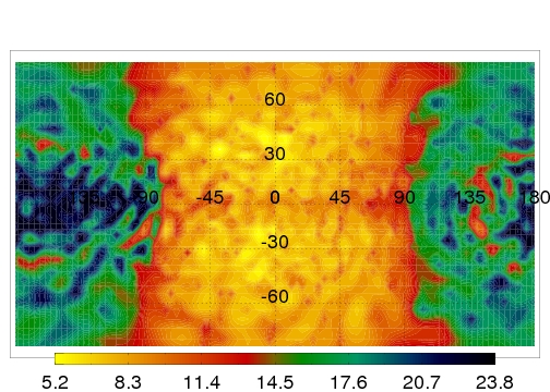
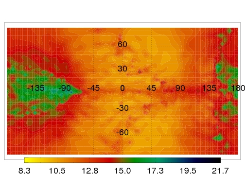
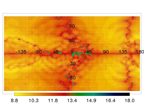
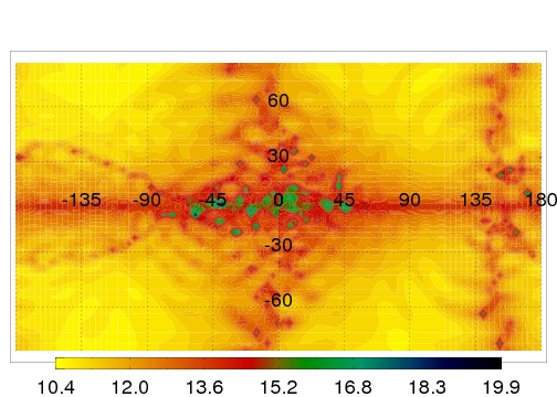
Figure 1.— Cylindrical maps of Joule heating times ($\log\tau_{J}$, in sec), at four pressure levels in our fiducial, drag-free atmospheric model. The sub-stellar point is centered at longitude and latitude zero. From top to bottom, Joule heating times are shown at 1 mbar, 50 mbar, 2 bar, 90 bar. Ohmic dissipation is not spatially uniform and it can dominate over heating by stellar insolation at deep enough pressure levels ($p\mathrel{\hbox to0.0pt{\lower 4.0pt\hbox{\hskip 1.0pt$\sim$}\hss}\raise 1.0pt\hbox{$>$}}2$ bars), where a new form of Joule-driven circulation could emerge. The calculation was performed for $B=3$ G, but note that ohmic dissipation increases steeply with magnetic field strength ($\tau_{J}\propto B^{-2}$).

2.2. Induced currents and Ohmic dissipation

The first step towards the computation of currents involves an estimate of the importance of various non-ideal MHD terms in the full induction equation for the weakly-ionized medium. For the atmospheric models under consideration here, PMR10 found that, for a surface magnetic field strength of 3 G, the Hall term is completely negligible throughout the flow, while the resistive term largely dominates over the ambipolar diffusion term everywhere except possibly in the model uppermost levels. Therefore, to a good approximation, the induction equation can be considered as purely resistive. Assuming that zonal winds are dominant, one needs only to consider the toroidal component of the induction equation

$$\frac{\partial B_{\phi}}{\partial t} = r\sin\theta\left[\frac{\partial\Omega}{\partial r}B_{r}+\frac{1}{r}\frac{\partial\Omega}{\partial\theta}B_{\theta}\right]+\frac{1}{r}\frac{\partial}{\partial r}\left[\eta\frac{\partial}{\partial r}(rB_{\phi})\right]$$ (4)

$$+ \frac{1}{r^{2}}\frac{\partial}{\partial\theta}\left[\frac{\eta}{\sin\theta}\frac{\partial}{\partial\theta}(\sin\theta B_{\phi})\right]\;,$$

where $\Omega={\rm v}_{\phi}(r\sin\theta)^{-1}$ is the local angular velocity of the flow, $r$ is the radial spherical coordinate, and the magnetic field is assumed to be an axisymmetric dipole.

In PMR10, we also argued that, to leading order, the latitudinal component of the current induced by the zonal flow should be dominant. This assumption could be verified in more general versions of our models. Since the magnetic Reynolds number is $R_{m}\ll 1$ for the bulk of the flow, no significant dynamo action is expected in the atmosphere. The dipolar planetary field $(B_{r},B_{\theta})$ is maintained by currents in the interior of the planet, while the zonal flows separately induce a $B_{\phi}$ component from the dipolar one in the superficial atmospheric layers. Under these conditions (Liu et al. 2008), the resulting steady-state latitudinal current can be computed as:

$$j_{\theta}(r,\theta,\phi) = -\frac{c\sin\theta}{4\pi r\eta(r,\theta,\phi)}\int_{r}^{R}dr^{\prime}{r^{\prime}}^{2}\left(\frac{\partial\Omega}{\partial r^{\prime}}B_{r}+\frac{1}{r^{\prime}}\frac{\partial\Omega}{\partial\theta}B_{\theta}\right)$$ (5)

$$+ \frac{R\eta(R,\theta,\phi)}{r\eta(r,\theta,\phi)}j_{\theta}(R,\theta,\phi)\;,$$

where the last term includes a boundary current in the uppermost modeled level, $j_{\theta}(R,\theta,\phi)$. Lacking information about the nature of currents possibly flowing from regions above the modeled atmospheric layers, we set this boundary current to zero for simplicity. As discussed in PMR10, this unknown boundary current represents an important source of uncertainty in our modeling, but, unless near cancellations occur, additional boundary currents could in principle contribute to even stronger ohmic dissipation than estimated here.

The ohmic power per unit volume dissipated locally is readily computed as (e.g., Liu et al. 2008)

$$Q_{J}(r,\theta,\phi)=\frac{[{j_{\theta}(r,\theta,\phi)}]^{2}}{\sigma_{e}(r,\theta,\phi)}\;.$$ (6)

2.3. Joule-driven Circulation

We first examine the possibility that spatially non-uniform ohmic dissipation drives a circulation in regions of the atmosphere where it is comparable or stronger than heating due to stellar insolation. To permit a direct comparison between the two heating sources, we find it convenient to define a typical local timescale associated with Joule heating, which is deduced from the energy equation

$$\rho\,C_{p}\,\frac{dT}{dt}=Q_{J}\,,$$ (7)

so that the Joule heating time is

$$\tau_{J}\sim\frac{\rho\,C_{p}\,T}{Q_{J}}\;.$$ (8)

The specific heat of the gas in our model atmospheres is $C_{p}=1.43\times 10^{8}$ erg g^-1 K^-1.

Fig. 1 shows cylindrical maps of Joule heating times for a nominal surface dipolar field of 3 G, at four depths in the atmospheric flow of our fiducial, drag-free model. In the uppermost levels, the Joule heating times span almost 20 orders of magnitude, with the shortest times found on the day side. This wide span reflects the large variations in resistivity, $\eta$, between the day and the night sides. On the day side, which has higher temperatures, $\eta$ is considerably smaller than on the night side, yielding larger currents, which in turn result in larger $Q_{J}$ and correspondingly smaller $\tau_{J}$ values. On the other hand, deep in the inert layers, which are little affected by stellar irradiation, Joule heating times span a more modest range of values, $\sim 10^{9}-10^{12}$ s over a large fraction of the flow. Longer timescales along the equator in the deeper levels are mostly the result of geometric effects: in Eq.(5), the term $(\partial\Omega/\partial r)B_{r}$ generally dominates over $1/r(\partial\Omega/\partial\theta)B_{\theta}$. Since $\Omega\propto\sin^{-1}\theta$ and $B_{r}\propto\cos\theta$, the net result is $j\propto\cos\theta$, and hence $\tau_{J}\propto\cos^{-2}\theta$. For a non-axisymmetric dipolar field, the anisotropy pattern would be different.

To evaluate the possibility of Joule-driven circulation, we compare local Joule heating times with a representative heating time associated with stellar irradiation, $\tau_{\rm irr}$. For consistency with the Newtonian forcing scheme used in our atmospheric models, we adopt a simple downward insolation flux that approximately matches the absorption properties of the one-dimensional models computed by Iro et al. (2005) at a few bars level. The flux is taken to obey $F(p)=F_{0}\exp[-4.5p/(2{\rm bar})]$, where $F_{0}=2.23\times 10^{8}$ erg cm^-2 ${s}^{-1}$ is the incident flux at the model top for HD 209458b, after geometric dilution by a factor $1/4$ as is customary for 1D-averaged models (e.g., Hansen 2008). A stellar irradiation heating timescale, $\tau_{\rm irr}$, is then computed following Eq. (8), with a heating rate taken as the vertical divergence of the stellar irradiation flux, $Q_{\rm irr}=-dF(r)/dr$. This allows us to evaluate $\tau_{\rm irr}$ simply as a function of the local pressure, pressure scale height and density. For example, at $p=2$ bar, using $\rho\sim 5.5\times 10^{-5}$ g cm^-3, we estimate $\tau_{\rm irr}\sim 5\times 10^{7}$ s. At $p=10$ bar, where the stellar insolation flux has been very strongly attenuated already (Iro et al. 2005), we estimate $\tau_{\rm irr}\sim 6\times 10^{15}$ s for $\rho\sim 3\times 10^{-4}$ g cm^-3. Deeper in the atmosphere, the insolation flux is further attenuated (exponentially so) and heating by insolation becomes largely inconsequential.

A comparison between values for $\tau_{\rm irr}$ and the detailed maps of $\tau_{J}$ values in Fig. 1 shows that, for the nominal $B=3$ G used in our $\tau_{J}$ calculation, irradiation dominates over Joule heating ($\tau_{\rm irr}\ll\tau_{J}$) everywhere on the day side of the atmosphere at pressure levels above a few bars. In these upper regions, we expect the atmospheric thermal structure to be largely unaffected by the extra Ohmic heating. Deeper than a few bars, however, Joule heating times start becoming comparable to or shorter than the typical heating time associated with stellar insolation, over significant regions of the atmospheric flow. Eventually, at levels deeper than about 10 bar, ohmic dissipation easily dominates over stellar insolation over much of the atmosphere. Since this extra source of heating in the deeper regions of the atmosphere is spatially non-uniform (Fig. 1), it should lead to some form of Joule-driven circulation in the “inert” layers located well below the radiatively-forced “weather” layers. This conclusion is largely independent of the specific stellar insolation model adopted here since the existence of radiatively inactive layers at levels deeper than a few bars is a rather generic property of irradiated hot Jupiter atmospheres (e.g., Hansen 2008). However, it remains to be seen what the nature of such Joule-driven circulation might be given the uneven heating pattern shown in Fig. 1, the non-uniformity of stellar insolation from the day-side to the night-side and the presence of an additional, spatially uniform net flux emerging from the deep planetary interior. Finally, it is worth remembering that, since $\tau_{J}\propto B^{-2}$, a stronger field could produce a substantially more dominant ohmic dissipation than estimated above for $B=3$ G.

2.4. Inflating Hot Jupiters

Another potentially important consequence of ohmic dissipation is the possibility that it contributes to the tendency for hot Jupiters to have inflated radii (Batygin & Stevenson 2010). To evaluate the magnitude of this effect on the basis of our three-dimensional atmospheric models, we compute the cumulative ohmic power dissipated in successive atmospheric shells, from the top level at a pressure $p_{t}$ of 1 mbar, down to a pressure $p(r)$ within the atmosphere; this is readily obtained by integration of Eq.(6),

$$P_{J}(p)=\int_{r(p)}^{r(p_{t})}dr^{\prime}{r^{\prime}}^{2}\int_{0}^{2\pi}d\phi\int_{0}^{\pi}d\theta\;\frac{[{j_{\theta}(r^{\prime},\theta,\phi)}]^{2}}{\sigma_{e}(r^{\prime},\theta,\phi)}\;.$$ (9)

Note that the power as computed above includes a horizontal average over the day and night sides. This averaging washes out the horizontal features in Joule heating shown in Fig. 1, an issue deserving further attention in future multi-dimensional models. Fig. 2 displays this ohmic power as a function of pressure for our fiducial, drag-free atmospheric model and for the model with strongest drag described in PMR10, with zonal wind speeds typically reduced by about $30-50\%$. For each model, we display ohmic power for two different values of the magnetic field strength adopted in the ohmic dissipation calculation, $B=3$ G, and $B=10$ G. This allows us to separately explore the effects of drag on the zonal winds and of the magnetic field strength on the resulting magnitude of ohmic dissipation. This is a useful exercise until models with a self-consistent treatment of magnetic drag and ohmic dissipation become available.

Fig. 2 shows that much of the dissipated ohmic power builds up at pressure levels from a few bars to several tens of bars. The power scales as $B^{2}$ and, relative to the drag-free model, it is reduced by a factor $\sim 3$ in the circulation model with strongly dragged winds, at fixed magnetic field strength. Since the stellar insolation power received by HD 209458b is $\sim 3\times 10^{22}$ W, Fig. 2 shows that the total ohmic power dissipated in these model atmospheres typically approaches or exceeds 1% of the stellar insolation power. Notice that, while the Ohmic power in Fig.2 is integrated down to the lowest grid points ($\sim 200$ bar) available in the model of Rauscher & Menou (2010), it is not yet seen to saturate at those levels. This is because, while the zonal velocities decrease with depth, they are still non-zero in the deepest, ’inert’ model layers. It is in fact not a priori clear where exactly the transition to the convection zone should be located in hot Jupiters and this constitutes an uncertainty for Joule heating models of the deepest atmospheric layers.

Overall, our results on the dissipated ohmic power are consistent with the estimates made by Batygin & Stevenson (2010) on the basis of a more idealized, one-dimensional atmosphere model, using a parametrized zonal wind profile. Like them, we find that a large fraction of the ohmic power is dissipated in the deeper atmospheric levels, below $\sim 10$ bar.

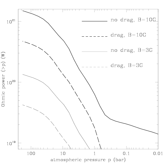
Figure 2.— Cumulative ohmic power dissipated above pressure level $p$, in four different models for HD 209458b. The solid lines correspond to the drag-free model described in Rauscher & Menou (2010) while the dashed lines correspond to the model with strongest drag, and reduced winds, described in Perna et al. (2010). Curves are labeled with the value of the magnetic field adopted for the ohmic dissipation calculation. The ohmic power can reach or exceed 1% of the stellar insolation power, $\sim 3\times 10^{22}$ W, in the deepest atmospheric layers, in models with and without dragged winds.

Contrary to Batygin & Stevenson (2010), however, we do not solve for radial currents in our models, only meridional ones (Eq. 5), and our results are thus largely independent of the presence or absence of an insulating layer high in the atmosphere. In fact, we find that an insulating layer is present on the nightside in our three-dimensional models, but not necessarily on the much hotter, less resistive dayside. This raises the possibility that, in more detailed three-dimensional MHD models, current loops could actually close high in the atmosphere, rather than deep in the planetary interior as conjectured by Batygin & Stevenson (2010). While our results, relying on leading-order meridional currents in the atmospheric region alone, are presumably not strongly sensitive to these conditions affecting radial currents, it remains to be seen how currents would flow in more realistic non-axisymmetric and three-dimensional models.

Various authors have evaluated the extra power that needs to be continuously dissipated deep in the convective interior of hot Jupiters to explain their inflated radii (e.g., Gu, Bodenheimer & Lin 2004, Burrows et al. 2007, Ibgui et al. 2009). While Batygin & Stevenson (2010) emphasize such a deep deposition scenario, our own ohmic dissipation models say little about this scenario since we only calculate currents and ohmic dissipation in the superficial atmospheric region of the planet. However, another means by which hot Jupiter radii can be inflated is by slowing down their rate of contraction, through modifications to the thermal structure of their overlaying atmospheres which act as boundary conditions for the cooling isentropic interiors. Indeed, Guillot & Showman (2002) argue that, if $\sim 1\%$ of the stellar insolation flux were deposited at pressures of tens of bars deep in the atmosphere, this would slow down cooling sufficiently to explain the inflated radii of hot Jupiters. While Guillot & Showman (2002) suggested that a downward flux of kinetic energy could in principle achieve such energy deposition, our Fig. 2 indicates that this is in fact naturally achieved by ohmic dissipation in our atmospheric models, with or without drag, for a magnetic field strength $B\mathrel{\hbox to0.0pt{\lower 4.0pt\hbox{\hskip 1.0pt$\sim$}\hss}\raise 1.0pt\hbox{$>$}}10$ G.

More specifically, Guillot & Showman (2002) describe an evolutionary model in which $2.4\times 10^{20}$ W are deposited at a location centered around 21 bar in the atmosphere of HD 209458b, which can explain its observed inflated radius. This is achieved by the two ohmic dissipation models represented by the upper dashed and solid lines in our Fig. 2. In fact, since even more ohmic power is dissipated deeper in, we anticipate that models with fields even weaker than $10$ G, possibly as low as 3 G, will be able to meet the inflated radius requirement for HD 209458b. This leads us to conclude that ohmic dissipation deep in the atmospheres of hot Jupiters, which indirectly taps into the kinetic energy of dragged winds driven by stellar insolation higher up, is a promising scenario to explain the inflated radii of hot Jupiters.

3. Summary and Conclusions

In this Letter, we have computed the rate of ohmic dissipation in representative, three-dimensional atmospheric circulation models of the hot Jupiter HD 209458b. We find that, for a fiducial magnetic field strength of 3 G, ohmic dissipation starts dominating over stellar insolation heating at levels deeper than a few bars. The spatial non-uniformity of this extra source of heat could induce Joule-driven circulation in the deep layers traditionally considered as “inert”. For a magnetic field strength $\mathrel{\hbox to0.0pt{\lower 4.0pt\hbox{\hskip 1.0pt$\sim$}\hss}\raise 1.0pt\hbox{$>$}}10$ G, our models also indicate that enough heat is deposited at pressures of several tens of bars to slow down cooling sufficiently that the inflated radii of hot Jupiters can be explained.

Our results hence suggest that magnetic interactions in hot Jupiter atmospheres play a fundamental coupling role for the dynamics and the thermal evolution of these planets. As such, our work calls for the problem to be treated more consistently: magnetic drag affects wind speeds and induces currents, while the ohmic dissipation of these currents can generate a deep atmospheric circulation which could, in turn, feedback on the circulation higher up. Indeed, the extra heat source might also enhance convection in the night side, which might in turn enhance cooling. These various ingredients will have to be incorporated consistently in circulation models for a better assessment of their influence on the structure and the evolution of hot Jupiters. Some diversity may naturally arise from variations in the magnetic field strength and geometry of different planets.

References

- (1)
- (2) Baraffe, I., Chabrier, G., Barman, T. 2010, Reports on Progress in Physics, Vol. 73, Issue 1, pp. 016901
- (3)
- (4) Batygin, K., Stevenson, D. J. 2010, ApJL, 714L, 238
- (5)
- (6) Burrows, A., Orton, G. to appear in “Exoplanets”, Spring 2010 Space Science Series of the University of Arizona Press (Tucson, AZ); Ed. S. Seager; eprint arXiv: 0910.0248
- (7)
- (8) Burrows, A., Hubeny, I., Budaj, J., & Hubbard, W. B. 2003, ApJ, 594, 545
- (9) Burrows, A., Rauscher, E., Spiegel, D. S., & Menou, K., eprint arXiv:1005.0346
- (10)
- (11) Charbonneau, D., Brown, T., M., lathm, D. W., & Mayor, M. 2000, ApJ, 529, L45
- (12)
- (13) Christensen, U. R., Holzwarth, V. & Reiners, A. 2009, Nat., 457, 167
- (14)
- (15) Cooper, C. S. & Showman, A. P. 2005, ApJ, 629, L45
- (16)
- (17) Dobbs-Dixon, I., Lin, D. N. C. 2008, ApJ, 673, 513
- (18)
- (19) Draine, B. T., Roberge, W. G., Dalgarno, A. 1983, ApJ, 264, 485
- (20)
- (21) Hansen, B. M. S. 2008, ApJS, 179, 484
- (22)
- (23) Gu, P.-G., Bodenheimer, P. H. & Lin, D. N. C. 2004, ApJ 608, 1076
- (24)
- (25) Guillot, T., Showman, A. P. 2002, A&A, 385, 156
- (26)
- (27) Ibgui, L., Spiegel, D. S. & Burrows, A. 2009, eprint ArXiv:0910.5928
- (28)
- (29) Iro, N., Bezard, B., & Guillot, T. 2005, A&A, 719, 727
- (30)
- (31) Laine, R. O., Lin, D. N. C., Dong, S. 2008, ApJ, 685, 521
- (32)
- (33) Liu, J., Goldreich, P. M., Stevenson, D. J. 2008, Icar., 653, 664
- (34)
- (35) Perna, R., Menou, K., Rauscher, E., 2010, ApJ, 719, 1421
- (36)
- (37) Rauscher, E. Menou, K. 2010, ApJ, 714, 1334
- (38)
- (39) Sanchez-Lavega, A. 2004, ApJ, 609, L87
- (40)
- (41) Seager, S. & Deming, D. 2010, ARA&A in press, arXiv:1005.4037
- (42)
- (43) Showman, A. P., Y-K. Cho, J., Menou, K. 2010, to appear in “Exoplanets”, Spring 2010 Space Science Series of the University of Arizona Press (Tucson, AZ); Ed. S. Seager; eprint arXiv: 0911.3170.
- (44)
- (45) Showman, A. P. et al. 2009, ApJ 699, 564
- (46)