Star Formation Histories in a Cluster Environment at $z\sim 0.84$

Abstract

We present a spectrophotometric analysis of galaxies belonging to the dynamically young, massive cluster RX J0152.7-1357 at $z\sim 0.84$, aimed at understanding the effects of the cluster environment on the star formation history (SFH) of cluster galaxies and the assembly of the red-sequence (RS). We use VLT/FORS spectroscopy, ACS/WFC optical and NTT/SofI near-IR data to characterize SFHs as a function of color, luminosity, morphology, stellar mass, and local environment from a sample of 134 spectroscopic members. In order to increase the signal-to-noise, individual galaxy spectra are stacked according to these properties. Moreover, the D4000, Balmer, CN3883, Fe4383 and C4668 indices are also quantified. The SFH analysis shows that galaxies in the blue faint-end of the RS have on average younger stars ($\Delta t\sim 2$ Gyr) than those in the red bright-end. We also found, for a given luminosity range, differences in age ($\Delta t\sim 0.5-1.3$ Gyr) as a function of color, indicating that the intrinsic scatter of the RS may be due to age variations. Passive galaxies in the blue faint-end of the RS are preferentially located in the low density areas of the cluster, likely being objects entering the RS from the “blue cloud”. It is likely that the quenching of the star formation of these RS galaxies is due to interaction with the intracluster medium. Furthermore, the SFH of galaxies in the RS as a function of stellar mass reveals signatures of “downsizing” in the overall cluster.

1. Introduction

There is no doubt that galaxy evolution is influenced by the local environment. The observed properties of galaxies (color, magnitude, morphology, metallicity) are associated with their local neighborhood. The latter is usually characterized in terms of the local number density of galaxies.

One of the most prominent connections between galaxy properties and environment is the morphology-density relation (Dressler, 1980), by which early-type galaxies dominate high-density environments in contrast to late-type galaxies that dominate low-density ones. This relation has been quantified up to $z\sim 1$, showing different evolutionary patterns depending on whether the galaxy sample is selected based on luminosity (Postman et al., 2005; Smith et al., 2005) or stellar mass (Holden et al., 2007; van der Wel et al., 2007).

For mass selected samples, van der Wel et al. (2007) show that galaxies have to evolve in mass, morphology, and density such that the morphology-density relation does not change since at least $z\sim 0.8$. In the case of luminosity-selected samples, the morphology-density relation observed at $z\sim 1$ (Postman et al., 2005) is reported to hold up to $z\sim 1.46$ (Hilton et al., 2009).

Since early-type galaxies are among the reddest objects in any given sample at a given epoch and contain the bulk of the stellar mass in the Universe, the above morphology-density relation can be translated into two other relations: color-density and stellar mass-density. In particular, the color-density relation, characterized by the tendency of red galaxies (mostly early-type ones) to be found in the core of clusters, can be used as a tool to identify high-redshift clusters. It takes advantage of one of the most distinctive features in the color-magnitude diagram of a cluster: the so-called red-sequence (RS; de Vaucouleurs, 1961; Visvanathan & Sandage, 1977).

This RS, however, is not exclusive of clusters as it is also found in the field. In fact, some of the observed properties of the RS such as its color scatter and luminosity coverage vary, at a given redshift, with local galaxy density (e.g., Tanaka et al., 2005). This highlights the influence that the local environment has on galaxy properties such as colors.

It has been observed that the RS of clusters has a small scatter in color and a slope which do not seem to evolve over $\sim 9$ Gyr of cosmic time since $z\sim 1.4$ (e.g., Stanford et al., 1998; Blakeslee et al., 2003b; Mei et al., 2006b; Lidman et al., 2008). This lack of evolution was shown to be better explained by a RS being primarily a color-metallicity relation instead of a color-age one (Kodama & Arimoto, 1997). However, more recent evidence gathered from local samples of galaxies shows that variations of stellar age along the red-sequence are also present (e.g., Gallazzi et al., 2006; Bernardi et al., 2006) in addition to variations in metallicity, with some of the intrinsic color scatter of the red-sequence being due to stellar age differences (see also Tran et al., 2007).

A common procedure is to use the spectral energy distribution (SED) fitting technique to estimate ages and formation redshifts for cluster galaxies in the RS (e.g., Blakeslee et al., 2003b; Lidman et al., 2004, 2008; Blakeslee et al., 2006; Mei et al., 2006a, b; Gobat et al., 2008; Rettura et al., 2010). This procedure allow us to constrain the epoch and mode of formation of massive early-type galaxies. When spectroscopic data allow it, spectral indices are also measured to constrain the properties and evolution of cluster galaxies (e.g., Jørgensen et al., 2005; Tran et al., 2007; Braglia et al., 2009).

At $z=1.2$, Gobat et al. (2008) find that the bulk of the stars in cluster early-type galaxies is formed $\sim$ 0.5 Gyr earlier than that in field early-type galaxies, and RS galaxies were already in place $\sim 1$ Gyr earlier. Although the most massive (in stellar content) early-type galaxies do not show such an age difference with environment, this age divergence is most noticeable at stellar masses $\lesssim 10^{11}M_{\odot}$. A similar conclusion was reached by Rettura et al. (2010), who show that the environment regulates the timescale associated with the SFHs of early-type galaxies, with a fraction of field system having a more extended period of stellar mass assembly.

Braglia et al. (2009) find that the SFHs of galaxies in two clusters at $z\sim 0.3$ depend on local environment which is also related to the cluster dynamical state. In addition to the expected gradient of star formation with clustercentric distance, both luminous ($L\geq L^{*}$) and sub-luminous members contribute to a sharp increase of the star formation activity along filaments connected to the dynamically young, merging system. The more relaxed cluster, on the other hand, is mostly dominated by red, passive galaxies or galaxies whose star formation is being quenched.

The novel procedure used by Gobat et al. (2008) to determine the SFH of cluster galaxies combines both the SED fitting technique and, simultaneously, a fit to the spectroscopic features (pseudo-continuum and absorption) of a galaxy spectrum. The SED covers a wide range of wavelengths and provides information on mass and current SFH while the spectrum, although on a much more limited wavelength range, allows one to determine the age of the stellar population of a galaxy with greater precision. The combination of photometry and spectroscopy therefore puts stronger constraints on the SFH than either alone. This approach can also be complemented by determining some relevant spectral indices available at the observed wavelength range.

The galaxy cluster RX J0152.7-1357 (Della Ceca et al., 2000) at $z\sim 0.84$, with its dynamically young and complex structure, represents and ideal laboratory to study the relation between galaxy SFH and environment. Here we apply the above spectrophotometric fitting technique to the spectroscopically confirmed population of cluster members. Our goal is to deepen our understanding of how galaxy evolution is driven by environmental processes and, in particular, to better constrain and understand the physical mechanisms that contribute to form the RS and set its observed properties.

RX J0152.7-1357 is one of the most distant X-ray luminous clusters discovered in the ROSAT Deep Cluster Survey (Rosati et al., 1998). It is observed at an epoch of greater cosmic activity in terms of stellar mass buildup in galaxies (e.g., Doherty et al., 2006), with the cluster itself being assembled by the merging of two subclusters (Demarco et al., 2005; Girardi et al., 2005) and by the accretion of groups from surrounding filaments (Tanaka et al., 2006).

To date, RX J0152.7-1357 has been the subject of a number of studies: ICM structure and X-ray properties (Maughan et al., 2003), RS properties (Blakeslee et al., 2006; Patel et al., 2009), cluster dynamics and substructure (Demarco et al., 2005; Girardi et al., 2005), star-forming members (Homeier et al., 2005), Sunyaev-Zel’dovich properties (Joy et al., 2001), weak lensing mass structure (Jee et al., 2005), physical properties of galaxy members (Jørgensen et al., 2005), infrared sources in the cluster (Marcillac et al., 2007), and large-scale filaments associated with it (Tanaka et al., 2006). It is one of the clusters in the ACS intermediate-redshift cluster program (Ford et al., 2004) with one of the most comprehensive datasets, from X-ray to infrared.

We improve over previous studies of this cluster by considering, simultaneously, a large enough ($\sim 130$) number of spectroscopic members with high enough ($<15$ Å) spectral resolution data and 5-band photometry (from optical to near-infrared). In addition, we characterize the local environment by the relative, projected dark matter density instead of the local projected number density of galaxies. We estimate SFHs and spectral indices as a function of color-magnitude, morphology, stellar mass and location within the cluster, which allows us to establish a comprehensive view of galaxy properties and their connection with the environment. In contrast to other works at this redshift, given the available number of members in the RS, we divide this one into a grid in color-magnitude space where the average SFH of galaxies can be studied at different colors and magnitudes. This approach is aimed at providing a deeper insight into RS variations in order to unveil the physics responsible of its observed properties such as its intrinsic scatter.

The present work is structured in the following way. In §2 we describe the observations and the dataset used in our analyses. In §3 we focus on the technical details of this investigation, such as the definition of regions in the hyperspace of galaxy properties considered for this investigation, the available spectra, the spectrophotometric fitting procedure used to characterize the average SFH within those regions, and the spectral indices used to complement such SFH characterization. In §4 we present the results of our analyses followed, in §5 by a discussion focused on the formation of the RS in the cluster. We finally summarize our main conclusions in §6.

Throughout the paper, unless explicitly indicated, we assume a $\Lambda$CDM cosmology with H${}_{0}=70$ km s^-1 Mpc^-1, $\Omega_{M}=0.3$ and $\Omega_{\Lambda}=0.7$.

2. Observations

RX J0152.7-1357 has been observed with a number of instruments from the ground and space. In this work we have used optical and near-IR imaging data obtained with HST/ACS and NTT/SofI, respectively, and optical spectroscopy obtained with VLT/FORS. Descriptions of these observations and data reductions can be found in the existing literature (Demarco et al., 2005; Blakeslee et al., 2006), hence, we only provide a short summary of them below.

2.1. Imaging and photometry

As reported in Blakeslee et al. (2006), RX J0152.7-1357 was observed with ACS (Ford et al., 1998) on HST in three bands: F625W, F775W and F850LP, hereafter referred to as $r_{625}$, $i_{775}$ and $z_{850}$, respectively. The cluster was imaged using a 2 $\times$ 2 overlapping pattern, producing a mosaic of about 5$\farcm$8 on a side with a central overlapping region of about 1′. Each pointing was observed for two orbits per filter, giving a total orbit expenditure of 24 orbits. The images were processed and the final mosaic produced using the ACS GTO Apsis pipeline (Blakeslee et al., 2003a). For more details, see Blakeslee et al. (2006).

The near-IR data were obtained with SofI (Moorwood et al., 1998) on the ESO NTT (see Demarco et al., 2005). The cluster was imaged in the J and K_s bands under sub-arcsecond seeing for 3.8 and 3 hours, respectively. The final images cover a region of 4$\farcm$9 on a side and were reduced in a standard manner.

In order to use the ACS and SofI data in a consistent way, we produced a new multi-band photometric catalog, different from those used in Demarco et al. (2005) (SofI) and Blakeslee et al. (2006) (ACS). Photometry from the ACS data was obtained in dual mode using the ACS $z_{850}$ image for detections. By running SExtractor (Bertin & Arnouts, 1996) on the ACS mosaic, 41 point sources were selected to derive aperture corrections. Magnitudes (in the AB system; Oke, 1974) within radii of 0$\farcs$75 and 2$\farcs$0 were compared, resulting in differences of 0.039 for both the $r_{625}$ and $i_{775}$ bands and 0.046 for the $z_{850}$ filter. Zero points (in AB magnitudes) for the $r_{625}$-, $i_{775}$- and $z_{850}$-band data are 36.542, 36.321 and 35.520, respectively.

The near-IR J and K_s images were registered onto the ACS ones, with residuals of less than 1 pixel for both J and K_s. The same point sources were used to derive corrections between apertures of 1″ and 5″ in radius. These corrections are 0.254 and 0.239 for J and K_s, respectively. Additionally, extinction corrections (Schlegel et al., 1998) of 0.014 in J and 0.009 in K were applied, resulting in a total correction for the 1″ radius aperture of 0.268 in J and 0.248 in K_s. Zero points (in the AB system) in J and K_s are 27.260 and 26.745, respectively. Hereafter, unless otherwise indicated, magnitudes are in the AB system. To transform the near-IR photometry from the Vega system to AB magnitudes, we used corrections of 0.960 and 1.895 for the J and K_s bands.

For completeness, we note that flanking fields surrounding the central $r_{625}$, $i_{775}$ and $z_{850}$ mosaic were obtained with ACS in F606W (broad V) and F814W (broad I), however, we did no attempt to use those data in this work because of their shallower integration, reduced photometric coverage, and lack of overlap with the existing near-IR data.

2.2. Spectroscopy

RX J0152.7-1357 and its outskirts have been subject of a number of extensive spectroscopic surveys (Demarco et al., 2005; Jørgensen et al., 2005; Tanaka et al., 2006; Patel et al., 2009). While the survey by Tanaka et al. (2006) concentrated on the large-scale structures surrounding the main cluster, only 8 members in Jørgensen’s survey were not included in Demarco’s work. In the present study, we use the spectra of the 102 cluster members confirmed by Demarco et al. (2005), complemented with the spectra of 32 new cluster members obtained from subsequent FORS2 (Appenzeller & Rupprecht, 1992) spectroscopy on the ESO VLT. These 134 sources are listed in table LABEL:tab_membs. IDs are in the same system of those in Demarco et al. (2005), and the last column corresponds to their emission line flag: a value of 0 is given to passive galaxies, a value of 1 is given to emission line galaxies, and a value of 2 is given to AGN.

The new 32 spectroscopic members were obtained after targeting clusters candidates with 4 multi-object masks, using the Mask Exchange Unit (MXU) on FORS2, and exposing each of them until reaching integration times between 3 and 4 hours. The data were collected between November 4th and November 7th, 2005, in Visitor Mode (ESO program ID 076.A-0889(A)) under an average seeing of $\sim 0\farcs 9$. A total of 152 galaxies were observed with slits of 1″ in width using the 300V grism. The data were binned by 2 pixels which resulted in a dispersion of $\sim 3.3$Å/pixel and a spectral resolution of $\sim 13$Å. One mask was observed using no order-separation filter while the other three masks were exposed using the GG375+80 filter. Although these observations were designed to target gravitational arc candidates, the new members resulted from putting the slits on fillers that were likely cluster members based on their photometric redshift ($0.7<z_{phot}<0.95$; see Demarco et al., 2005).

The observations were prepared and the data reduced in a similar way and using the same dedicated software as described in Demarco et al. (2005). Redshifts were obtained by cross-correlating (Tonry & Davis, 1979; Kurtz et al., 1992) the observed spectra with template galaxy spectra from Kinney et al. (1996). Out of 113 redshifts, 32 were securely confirmed within the range defining cluster membership ($0.81<z<0.87$; see Demarco et al., 2005). Observational errors (obtained from observing several sources more than once) are of the same order of magnitude as those reported in Demarco et al. (2005, 2007), i.e., $\delta z\sim 8-12\times 10^{-4}\sim 10^{-3}$.

3. Analysis

In an effort to better understand how galaxy properties, such as age and stellar mass, contribute to establishing the observed characteristics of the RS, we focus the present analysis on the star formation history (SFH) of cluster galaxies in the RS. As the luminosity coverage and scatter of the RS are observed to vary between cluster and field environment (e.g., Tanaka et al., 2005), we also investigate the impact that the intracluster environment may have on the above SFHs.

Traditionally, SFHs are determined by fitting synthetic galaxy spectra to the available photometry (e.g., Rettura et al., 2006, 2010), however, in the present analysis, we additionally perform a simultaneous fit to the available spectra as performed by Gobat et al. (2008). In order to increase signal-to-noise (S/N) for the spectrophotometric fitting, galaxy spectra are co-added as explained in §3.1. Before stacking, galaxy spectra are grouped according to color, magnitude, location within a given subcluster and with respect to the projected DM distribution, stellar mass, and visual morphology. All these grouping regions are defined in §3.2 and the details of the spectrophotometric fitting procedure are given in §3.4.

3.1. Co-added spectra

The individual spectra of the 134 cluster members of RX J0152.7-1357 used in the present analysis have S/N ratios in the range 1 to 33 with a mean value of 7.6. The S/N ratios were obtained from the ratio between the mean flux and the r.m.s. flux calculated within the wavelength intervals defining the continuum windows for the H$\delta_{A}$ feature (Worthey & Ottaviani, 1997). Since the redshift survey presented in Demarco et al. (2005) was designed to mainly provide redshifts, the quality of the individual spectra is not good enough to perform a meaningful fit to the different spectral features sensitive to the SFH. Therefore, in order to increase the S/N ratio to obtain a satisfactory SFH characterization, we decided to use average spectra obtained from co-adding individual spectra that were grouped according to various criteria (see §3.2).

This stacking technique has already been successfully used in previous studies about the stellar populations in cluster galaxies at intermediate-redshift (e.g., Dressler et al., 2004), and the algorithm employed here is the same as in Demarco et al. (2007) and Gobat et al. (2008). The individual spectra can be weighted by their S/N, and only those with a S/N $>3$ were selected for stacking. The S/N ratios of the final, co-added spectra vary between $\sim$6 and $\sim$42 for the unweighted stacking, and between $\sim$6 and $\sim$62 for the weighted stacking.

3.2. Grouping cluster members

SFHs are determined from co-added spectra grouped according to relevant observables. In this work we study their dependence on galaxy color and magnitude, projected angular distribution, visual morphology, stellar mass, and projected DM density. These observables can be considered as forming an hyperspace in which galaxies are located. The regions within this hyperspace used for stacking spectra are defined in what follows and table 2 summarizes all these definitions.

3.2.1 Galaxy colors and luminosities

Since we are interested in understanding the physical origin of the scatter of the RS in clusters, and ultimately the details of the color-luminosity evolution of cluster galaxies into the RS, we need first to separate cluster members into blue and red galaxies. We follow the traditional way of using two filters that straddle the 4000Å-break at the cluster redshift to achieve this. Fig. 1 shows a simple stellar population (SSP), 12 Gyr old, solar metallicity spectral energy distribution from the Bruzual-Charlot (Bruzual & Charlot, 2003) library, redshifted to the cluster redshift ($z=0.837$; Demarco et al., 2005). On top of it, our choice of filters ($r_{625}$ and K_s) to straddle the 4000Å-break is laid out, which allows us to separate in an efficient way red (early-type) from blue (late-type) galaxies. In contrast to Blakeslee et al. (2006), we prefer to use the K_s-band as a the “red” filter because of its ability to trace the rest-frame near-IR light coming from the bulk of the stellar content of galaxies at $z\sim 0.8$, unaffected by biases due to recent star formation (Stanford et al., 1998).

Fig. 2 shows the Color-Magnitude Diagram (CMD) of RX J0152.7-1357 (for a detailed analysis of the CMD of this cluster, see Blakeslee et al., 2006). Red circles correspond to passive (no detectable emission features) cluster members, black triangles correspond to star-forming (with detectable [O$\mathrm{II}$]) members, and the two blue squares are the confirmed AGN members (Demarco et al., 2005). The black dots are sources within the ACS mosaic for which photometric information is available, and the cross at the lower-left of the plot indicates typical error bars in magnitude and color. The horizontal dashed line has arbitrarily been set at $r_{625}-K_{s}=2.3$ to separate blue from red galaxies. We consider galaxies with a $r_{625}-K_{s}>2.3$ color as belonging to the cluster RS.

In order to better explore SFH variations as a function of color and magnitude within the RS, we have subdivided the latter into a number of regions. A first subdivision is defined, consisting of three bins in K_s magnitude, 1/BRS, 2/MRS and 3/FRS, as defined in table 2. In addition, a second and finer subdivision, both in color and magnitude, is established, as shown in Fig. 2. The vertical dashed line has arbitrarily been set at $K_{s}=20.75$ in order to divide the RS into “bright” and “faint” bins. For comparison, K${}^{*}\sim 19.7$ (AB) at $z\sim 0.84$ (see Ellis & Jones, 2004), therefore, this separation corresponds to $\sim K^{*}+1$.

The locus of the RS in Fig. 2 is obtained by a linear least-squares fit to the data in color-magnitude space with $r_{625}-K_{s}>2.3$ and $18<K_{s}<24$. This fit to the RS ($r_{625}-K_{s}=(-0.219\pm 0.001)\times K_{s}+(7.751\pm 0.026)$), indicated by the solid black line, is used to define the “blue”, “green” and “red” areas parallel to it in color-magnitude space, further separated into 3 bright (regions 4/BBRS, 5/BGRS and 6/BRRS, respectively) and 3 faint (regions 7/FBRS, 8/FGRS and 9/FRRS, respectively) bins (see table 2 for their definitions).

Only passive galaxies (red circles) within these 9 regions were considered for stacking, because of our interest in focusing on the quiescent, early-type galaxy population. In general red, star-forming sources are dust-enshrouded systems (e.g., Smail et al., 1999; Wolf et al., 2005). However, we note that a few of the apparently passive, RS galaxies could in fact be star-forming systems with the [O$\mathrm{II}$] feature totally suppressed by a large amount of dust (e.g., Smail et al., 1999).

The above color separation for galaxies in the RS does not follow the slope of the fit to the RS. Selecting galaxies following this slope would tend to include more galaxies into the blue faint-end of the RS that may belong to the so-called “green valley” or to the “blue cloud”. Since we are interested in passive galaxies in the RS, the flat color separation we have adopted produces no different result from a slope-driven color separation.

We have 76 spectra corresponding to non [O$\mathrm{II}$] emission line galaxies in the RS available for our analyses. In order to have a reasonable number of sources to be co-added, we set the width of the two (bright and faint) central regions (green hatched areas) of the finer partition to be 0.2 mag in $r_{625}-Ks$ ($\pm 0.1$ in $r_{625}-Ks$ from the fit), which is about $1.1$ times the observed r.m.s. color scatter.

3.2.2 Projected angular distribution

To investigate the relation between stellar content and local environment, we study the SFH of cluster galaxies as a function of angular distribution on the sky. Due to the complex matter (DM, gas and galaxies) distribution of RX J0152.7-1357 (Maughan et al., 2003; Demarco et al., 2005; Jee et al., 2005; Girardi et al., 2005), it is very difficult to determine the center of the cluster. Instead of stacking galaxies in concentric rings with a common center, we try the following approach that considers the known main subclusters (see Demarco et al., 2005; Girardi et al., 2005).

We separate the cluster field of view (FoV) in two halves at a fiducial center (R.A.= 01$h$52$m$41.80$s$, DEC.=-13^o57″52$\farcs$5) located at the mid-point between the centers of the northern and southern clumps defined by Demarco et al. (2005), as indicated by the dashed, horizontal line in Fig. 3. We then consider concentric (semi-)annuli or radial sectors centered at each clump, however, truncated at the separation half-way between them (solid contours in Fig. 3). Areas or sectors associated with the northern clump (20/N0 through 22/N2) are labeled as “North”, while those associated with the southern clump (23/S0 through 25/S2) are labeled as “South”. In table 2 we give the corresponding definitions of the above regions. The center of each clump or subcluster is taken from Demarco et al. (2005).

All galaxies, passive and those showing emission lines, were considered for stacking within these regions. We only excluded the known AGN members.

3.2.3 Galaxy morphology

We use the morphological classification given by Postman et al. (2005) for galaxies in RX J0152.7-1357. The morphological T-types used by Postman and collaborators are those defined in de Vaucouleurs et al. (1976). T values ranging from -5 to -3 correspond to Elliptical (E) galaxies, while a value of -2 corresponds to S0 galaxies. Values between -1 and 1 are assigned to morphologies between S0 and Sa, with values $>1$ given to later type spiral (Sp) galaxies. Type 6 is associated with a Sd morphology, while irregular (Irr) galaxies have T values in the range $6<T<9$. Taking all this under consideration, we established 4 groups in morphology space as defined in table 2. Namely, group 10/E contains elliptical galaxies ($T<-2$); group 11/(S0/Sa), lenticular galaxies ($-2\geq T\geq-1$); group 12/Sp, spiral galaxies ($1<T\leq 6$); and group 13/Irr, irregular galaxies ($T>6$).

3.2.4 Stellar mass

In addition to morphology, we also grouped galaxies based on their stellar mass content. The work by Holden et al. (2007) provides stellar mass estimates for cluster galaxies in RX J0152.7-1357 based on the mass-to-light, $M/L_{B}$, ratio and rest-frame $(B-V)$ color linear relation derived by Bell et al. (2003). Those masses, in despite of being based on a single color, are proven to be consistent with other estimates as shown by a comparison with dynamical measurements for some of the same galaxies (see Holden et al. (2007), and references therein).

However, in the analyses shown here, we decided to recompute stellar masses by using a SED fitting procedure (Rettura et al., 2006) including all the 5 bands available (see §2.1). This information allowed us to establish 3 bins in stellar mass (14/RSHM through 16/RSLM) as defined in table 2. Stellar masses span the range $4.8\times 10^{9}<M_{*}\leq 3.9\times 10^{11}\ M_{\odot}$, and the mass interval for each bin has been adjusted in order to have roughly the same number of spectra to co-add per bin. A more detailed explanation about the way these stellar masses were obtained is presented in §3.4. In order to study SFH variations with stellar mass for the same sample of RS galaxies in §3.2.1, we also restrict ourselves to quiescent, RS galaxies, i.e., those with colors $2.3<(r_{625}-K_{s})<4.5$ and no visible emission line features.

3.2.5 Local dark matter density

RX J0152.7-1357 has been the subject of a detailed weak lensing analysis by Jee et al. (2005). By using the available $r_{625}$, $i_{775}$ and $z_{850}$ ACS data together with photometric and spectroscopic (from Demarco et al., 2005) redshifts, they are able to measure the shear signal of the cluster and reconstruct its dimensionless mass density, $\kappa$. The smoothing scale of the map is $\sim 20$″, while its accuracy is about 20%.

As an alternative way of characterizing the cluster environment to that presented in §3.2.2, here we use the $\kappa$ map from Jee et al. (2005) to identify environments of different projected mass density in the ACS FoV of RX J0152.7-1357. Because of the so-called sheet-mass degeneracy, i.e., the invariance of the shear under transformations of the kind $\kappa\rightarrow\lambda\kappa+(1-\lambda)$, we use this $\kappa$ map in a relative sense, only, during the interpretation of the results.

We thus arbitrarily define 3 different environments based on their local, projected (total) mass density, as shown in Fig. 4. The first of them is characterized by mass densities $>20\times\sigma_{DM}$ (solid contours in Fig. 4), with $\sigma_{DM}=0.0057\times\Sigma_{c}$, being $\Sigma_{c}\sim 3650M_{\odot}\ pc^{-2}$ the critical mass density of the cluster (Blakeslee et al., 2006). The $\kappa$ value around the two brightest central galaxies of the northern clump (the cluster center adopted in Jee et al., 2005) is $\sim$0.3. The second one is that containing mass densities between 5 (dashed contours in Fig. 4) and 20 times $\sigma_{DM}$, while the last of the three encompasses mass densities $<5\times\sigma_{DM}$, reaching negative values in some areas. These three environments correspond to regions 17/HDMD, 18/MDMD, and 19/LDMD, respectively, as presented in table 2. Also in Fig. 4, the distribution of spectroscopic members is indicated by the symbols. Members in the highest density regions are indicated as squares; members in the intermediate density regions, as triangles; and members in the lowest density environments, as upside down triangles. For comparison, we also show the horizontal dashed line in Fig. 3 that contains the mid-point between the two main central sub-clusters.

As with the galaxies separated according to angular distribution, all non-emission and emission line galaxies, except the confirmed AGN members, were considered for stacking. The inclusion here of star-forming galaxies, as opposed to the regions in color-magnitude space and stellar mass that only include non-emission line objects, is because we are also interested in studying how the environment affects the cluster galaxy population as a whole (passive and star-forming galaxies; see §4.1.3). Environmental effects on the passive cluster galaxy population only is discussed in §4.1.3 and §5.

3.3. Weighted vs unweighted stacking

After stacking the spectra, we checked for differences between the co-added spectra obtained from weighting the individual sources by their corresponding S/N at $\sim 4100$ Å (rest-frame; see §3.1) and those obtained from a direct stacking without weights. The difference in S/N, $\Delta(S/N)$, as noted in §3.1 and as expected, favors the weight-stacked spectra.

With the exception of a few groups with only 2 to 3 spectra available for stacking, for which $\Delta(S/N)<1.6$, we note that the region containing the core of the northern clump (20/N0) has a $\Delta(S/N)\sim 0.5$. The S/N distribution of individual galaxies within 20/N0 is not specially different from that of many of the other regions, with a mean S/N of $\sim$ 8 and a $\sigma_{S/N}\sim 3$. Besides this, differences in S/N between the weight- and unweight-stacked spectra is $\Delta(S/N)>4$, with typical values of the order of 40%. Because of the improvement in S/N, the results that we present below are obtained from the weight-stacked spectra.

The resulting weight-stacked spectrum for each region in hyperspace is shown in the corresponding panel of Fig. 5 and Fig. 6 as the thick black line. Each spectrum is shown redshifted to mean cluster redshift of $z=0.837$ (Demarco et al., 2005). The relative flux is in arbitrary units.

3.4. Spectrophotometric fitting

As in Gobat et al. (2008), here we perform a fit to both the corresponding broad-band photometry and the stacked spectrum for each one of the regions defined in table 2. The broad-band magnitude for a given region of hyperspace in a given band is obtained from averaging the individual magnitudes of the sources in that region for that band. The photometric data are weighted by the corresponding photometric S/N of the object before staking.

In the present analysis, we have used a set of composite stellar populations models from the Bruzual & Charlot (2003) library, all with solar metallicity (see §4.4.1), and using the “Padova 1994” stellar tracks. While a newer, revised library exists (Girardi et al., 2000), it produces worse agreement with galaxy colors (Bruzual & Charlot, 2003) than the Padova 1994 library. Although the Gobat et al. (2008)’s code is able to handle both the Bruzual & Charlot (2003) and Maraston (2005) models, we prefer to use the former when fitting the co-added spectra because of their higher resolution ($\Delta\lambda\sim 6$ Å at $z=0.837$) when compared with the latter ($\Delta\lambda\sim 27$ Å at $z=0.837$), within the considered wavelength range. In this way, we degrade the resolution of the redshifted models instead of that of the data.

The model spectra are considered within the context of a delayed, exponentially declining SFH, without secondary episodes of star formation (see Gobat et al., 2008). These SFHs are parameterized by a time-scale $\tau$, therefore, they are referred to as “$\tau$-models”. We model the SED as a function of the time $T$ between 200 Myr to the age of the universe at the cluster redshift ($z=0.837$) in increments of $\sim$250 Myr. Different SFHs are characterized by $\tau$-models with $0<\tau<2$ Gyr in increments of 50 Myr, and we assume a Salpeter (1955) initial mass function (IMF) with mass cutoffs at 0.1 and 100 $M_{\odot}$ (see also Gobat et al., 2008). The averaged photometric data and co-added spectra, for each stacking region, are independently compared with the above grid of models using a $\chi^{2}$ statistics with $q$ degrees of freedom as defined in Avni (1976).

The number of degrees of freedom, $q$, for each spectrophotometric fit is defined as the number of independent variables minus the number of parameters. In the case of the spectroscopic data, the number of independent variables is difficult to estimate because of correlations between data points due to a spectral sampling finer than the FWHM resolution and a linearization of the wavelength solution. In order to take this into account, and as a good first-order approximation, we multiplied the $\chi^{2}$ value of the fit to the stacked spectrum by the ratio of the FWHM resolution to the sampling size within the considered wavelength range before estimating the confidence regions.

Since the true SFH of a galaxy may be more complex than a simple delayed exponential, and because the S/N of galaxy spectra at $z\sim 1$ often turns out to be relatively low, the $\tau$-model corresponding to the absolute minimum $\chi^{2}$ may not be sufficient to properly describe the actual SFH. Therefore, and in order to also be less sensitive to different systematic uncertainties from both the photometric and spectroscopic data, we consider models that are within the 99.7% confidence regions of the fits to the photometry and stacked spectra, in the space of model parameters.

Among the models within the intersection of the 99.7% confidence regions of the separate fits to the photometric and spectroscopic data, we consider as “best-fitting” model the one which has the lowest $\chi^{2}$ value for the fit to the observed co-added spectrum. In some cases this will be the actual, absolute best fit to the spectrum, but not always. The best-fitting model in each region of hyperspace is shown as the blue line in the corresponding panel of Fig. 5 and Fig. 6. In the same figures, the minimum and maximum fitting flux values within the above intersection, and as a function of wavelength, are represented by the green lines.

The $\chi^{2}$ statistics (Avni, 1976) is minimized with respect to the parameters of the model: $T$, $\tau$, and $M_{*,SED}$, the stellar mass (for the fit to the photometry), or $\sigma_{v}$, the stellar velocity dispersion (for the fit to the spectrum). The value of $\sigma_{v}$ is allowed to vary within the range 0 - 400 km/s. We calculate then the stellar age of a galaxy as its SFR-weighted age, $T_{SFR}$, defined as:

$$T_{SFR}(T,\tau)=\frac{\int^{T}_{0}(T-t)\psi(t,\tau)dt}{\int^{T}_{0}\psi(t,\tau)dt}\\ ,$$ (1)

where

$$\psi(t,\tau)=\frac{1}{\tau^{2}}\ te^{\frac{-t}{\tau}}$$ (2)

is the $\tau$-model giving the SFR as a function of time since the onset of the star formation. This definition takes into account the effective fraction of stellar mass contributed by each single stellar population making up the model spectrum, and stellar populations contributing only a negligible fraction to the stellar mass at any given time $T$ do not affect $T_{SFR}$ significantly.

We also define a second estimator, the final formation time, $t_{fin}$, as $M_{*}(t_{fin})=0.99\times M_{*}(T)$. In contrast to $T_{SFR}$, $t_{fin}$ is sensitive to the residual star formation. Hence, while $T_{SFR}$ measures the age of the bulk of the stars in a galaxy, $t_{fin}$ traces the last stages of stellar mass assembly, and is therefore useful to distinguish between two otherwise old stellar populations that have stopped star formation at different times. For a model spectrum that fits the observed broad-band photometry or spectrum of a galaxy, $T-t_{fin}$ corresponds to the lookback time from the epoch of the galaxy to the last episode of star formation, and is independent of the time at which the star formation of the $\tau$-model started.

We note that the results from the spectrophotometric fit are only weakly dependent on abundance, even though the Bruzual & Charlot (2003) models used here were computed at solar ratios only. This is due to the fact that we are also fitting several other spectral features which do not depend on [$\alpha$/Fe], such as Ca$\mathrm{II}$ H, Ca$\mathrm{II}$ K, D4000, G4300 (Thomas et al., 2003) and C4668 (e.g., Jørgensen et al., 2005). The first three, in particular, are the most prominent features in our stacked spectra and, therefore, drive the fit on the spectrum. We also make use of the 5-band SED, whose shape varies with age and metallicity but does not depend on individual absorption features. As a result, while the spectral features that do depend on $\alpha$-abundance might increase the best-fit $\chi^{2}$, their weight on the fit is greatly reduced.

In addition, we applied the above $\chi^{2}$ statistics to the individual 134 sources spectroscopically confirmed as cluster members. By fitting their photometric data as described earlier in this section, we are able to obtain the corresponding stellar mass, $M_{*,SED}$, which we compare with the value derived by Holden et al. (2007), $M_{*,(B-V)_{0}}$, based on the rest-frame B-V color, if available. Our photometric stellar masses are about a factor of two larger than those from Holden et al. (2007). A linear fit to the mass measurements gives $M_{*,SED}=(1.7\pm 0.27)\times M^{0.99\pm 0.3}_{*,(B-V)_{0}}$ (Gobat, 2009). The slight overestimate of the SED-derived masses with respect to those of Holden et al. (2007) might be due to the choice of the IMF. Likewise, if the metallicity of cluster galaxies is greater than solar, their SEDs would appear older when compared with a solar metallicity model. As a consequence, the fit would tend to overestimate the near-IR fluxes and thus the stellar masses. We considered our $M_{*,SED}$ values during the analyses.

3.5. Spectral features and indices

In addition to SFHs, we also computed line indices from the stacked spectra to characterize the stellar and metal content of cluster galaxies. At rest-frame optical wavelengths, the most prominent feature in the continuum of a galaxy produced by old, evolved ($\gtrsim 3$ Gyr; Poggianti & Barbaro, 1997) stars is the so-called 4000Å-Break (see, e.g., Bruzual A., 1983; Poggianti & Barbaro, 1997; Emerson, 1999). Younger stars, $\lesssim$ 2 Gyr, have a stronger flux density at wavelengths shorter than 4000 Å, producing a different discontinuity: the Balmer jump at 3646 Å (see Emerson, 1999).

In addition to the Balmer jump, stars with ages $\gtrsim 0.2$ Gyr also display large Balmer absorption lines such as H$\alpha$, H$\beta$, H$\gamma$, H$\delta$, H$\epsilon$, H6, etc. (e.g., Swinbank et al., 2005). The strength of these lines is maximum for A0V stars, but they can be detected from late-B to early-F type stars (Poggianti & Barbaro, 1997). The presence of deep Balmer lines is the signature of a young stellar population (e.g., Couch & Sharples, 1987; Poggianti et al., 1999).

As the stellar population ages, the main contribution to the flux shifts to cooler stars. The luminosity of the galaxy decreases, as does the depth of the Balmer lines, and the Balmer jump is replaced with the 4000 Å-break produced by line blanketing due to metals including CN and Ca$\mathrm{II}$ (e.g., Emerson, 1999). The strength of the 4000 Å-break increases with age and metal content and is, for a fixed metallicity, a measure of age (e.g., Poggianti & Barbaro, 1997; Kauffmann et al., 2003) and a good indicator of old populations of stars.

Because of the aforementioned metal absorption, the true continuum at some wavelengths cannot be measured, and the apparent strength of some of the high-order Balmer features (H$\delta$, H$\epsilon$, H6, etc.) becomes sensitive to the metal content and [$\alpha$/Fe] ratio of the stellar population (Maraston et al., 2003; Dressler et al., 2004; Thomas et al., 2004; Prochaska et al., 2007). Therefore, line indices based on such features have to be considered with caution when using them to quantify young stellar populations in galaxies. Another effect that may bias this quantification is that of the intrinsic velocity dispersion of the galaxy, however, of smaller magnitude (Kelson et al., 2006) compared with that of metallicity.

Very young ($<200$ Myr), massive ($>10M_{\odot}$) O- and B-type stars are able to ionize their surrounding gaseous medium, which translates in the presence of emission line features such as H$\alpha$, H$\beta$, [O$\mathrm{II}$] ($\lambda$$\lambda$3727) and [O$\mathrm{III}$] ($\lambda$4959,$\lambda$5007) in the optical window. Because of the short lifetimes of those massive, ionizing stars, these emission lines can be used to obtain a measure of the nearly instantaneus SFR, independent of the previous star formation history (Kennicutt, 1998).

Establishing the significance of the old stellar content of a galaxy is done my means of the D4000 index (Bruzual A., 1983) that measures the ratio between the continuum level at both sides of the 4000 Å-break. Here we use the modified version of it (Balogh et al., 1999, see table 3), which is based on narrower continuum windows. Although sensitive to metallicity effects, at early stages ($\lesssim 1$ Gyr) of stellar evolution, the D4000 index can be used as a good age indicator (Poggianti & Barbaro, 1997; Kauffmann et al., 2003). Assuming solar metallicity, stellar populations older than 3 Gyr are characterized by D4000 values $>1.7$ (Kauffmann et al., 2003).

The significance of young stars, between 1 and 2 Gyr old, is estimated from the equivalent width (EW) of some of the Balmer absorption lines (see, e.g., Couch & Sharples, 1987; Poggianti et al., 1999). Here we use the H$\delta_{A}$ index, as defined by Worthey & Ottaviani (1997). Following Dressler et al. (1999), we consider objects with EW(H$\delta_{A}$) $>4$ Å (see also Poggianti et al., 1999) as galaxies with a significant young stellar component. For younger ages, the [O$\mathrm{II}$] index defined in Tran et al. (2003) (see table 3) can be used as an indicator of current star-forming activity, keeping in mind its vulnerability to dust absorption. As in Dressler et al. (1999), we consider values of EW([O$\mathrm{II}$]) $\lesssim-5$ Å as significant. As shown recently for a supercluster environment at $z\sim 0.9$ (Lemaux et al., 2010), [O$\mathrm{II}$] emission can also be associated with a LINER or Seyfert component. Although it is something to bear in mind, we assume that this is not the case for our [O$\mathrm{II}$] emitters.

In addition to H$\delta_{A}$, we introduce a new index associated with the H6 ($\lambda$3889) Balmer line (e.g., van Dokkum & Stanford, 2003). The pseudo-continuum and line windows are given in table 3. We use a single stellar population, solar metallicity, 0.5 Gyr old model from the Bruzual-Charlot library (Bruzual & Charlot, 2003) in order to define the windows used to calculate the line EW. We note, however, that this definition becomes sensitive to the strength of CN when old stellar populations become more important in the galaxy spectrum.

Finally, in order to investigate trends with metallicity, we also computed indices of some metal features available in the wevelength range covered by our data: Fe4383 and C4668, as defined in Worthey et al. (1994), and CN3883, as defined in Davidge & Clark (1994) (see table 3).

Most of the absorption indices described above are measured here using the same window definitions of the Lick/IDS system (Worthey et al., 1994; Worthey & Ottaviani, 1997). However, our spectra have a resolution that is $\sim 3-5$ Å lower than those in the Lick/IDS system (Worthey & Ottaviani, 1997), therefore, a direct comparison to the Lick/IDS indices cannot be performed.

4. Results

4.1. Star Formation Histories

The spectrophotometric fitting procedure described in §3.4 allows us to characterize the SFH associated with the co-added photometry and spectra of the galaxies in each of the hyperspace regions defined in table 2. This characterization is given in terms of the SFR-weighted age, ($T_{SFR}$; see Eq. 1), the formation redshift ($z_{f}$), the final formation lookback time from $z=0.837$ ($T-t_{fin}$; see §3.4), and the final formation redshift ($z_{fin}$; see §3.4). The formation redshift, $z_{f}$, is defined as the redshift corresponding to $T_{SFR}$. The values of these parameters for the different regions defined in table 2 (see §3.2) are summarized in table 4. “Error” bars shown in Figures 7 through 10 actually indicate the maximum and minimum parameter values within the intersection of the 99.7% confidence regions of the fits to the composite SED and stacked spectrum.

When fitting the spectrophotometric data of bins that have a mix of early- and late-type galaxies, the adopted SFH may not be sufficient. Indeed, the spectrophotometry of those bins corresponds to a combination of old and young stellar populations, whose composite SFH may not be adequately parametrized by a simple delayed exponential. In addition, the [O$\mathrm{II}$] ($\lambda$3727) emission feature is enclosed by the $r_{625}$ band. This results in a higher $r_{625}$ flux and therefore in bluer colors. The best fitting models to the SED would then be younger than those to the spectrum, where the [O$\mathrm{II}$] line is ignored. This can lead to a significant discrepancy between the photometric and spectroscopic solutions, with no intersection in parameter space. In fact, no 99.7% intersection in parameter space was found for region 24/S1 (see table 4).

In what follows, we present our main results about the average SFH of cluster members in the RS, as well as in terms of stellar mass and environment, as defined in §3.2 (see table 2). Since SFHs are obtained by using solar metallicity models, in §4.4.1 we give a justification for this while in §4.4.2 we discuss about the biases introduced by this choice.

4.1.1 SFH in the cluster RS

Results from the three-bin partition are shown in panels (a) and (c) of Fig. 7. Panel (a) shows that the $T_{SFR}$ within the cluster RS decreases proportional to $K_{s}$ as $T_{SFR}=-0.7\times K_{s}+18.5$ Gyr. Panel (c) shows that the lookback time from the epoch of observation to the last episode of star formation, $T-t_{fin}$, varies as $T-t_{fin}=-1.0\times K_{s}+23.0$ Gyr. The other two panels in Fig. 7, (b) and (d), show the variations of $T_{SFR}$ and $T-t_{fin}$ with color as obtained from the finer RS partition. The Spearman’s rank test (Press et al., 1992) indicates that the trend between age and $r_{625}-K_{s}$ color (panel b) is significant with $>95$% significance ($\rho=0.99$). This correlation can be described as $T_{SFR}=2.4\times(r_{625}-K_{s})-4.0$ Gyr. In the case of the lookback time $T-t_{fin}$, the Spearman’s rank test also gives a significance $>95$ % ($\rho=0.94$) for the observed correlation with color. A linear fit shows that this correlation can be characterized as $T-t_{fin}=3.6\times(r_{625}-K_{s})-9.4$ Gyr.

The above correlations indicate that, on average, galaxies in the brighter and redder RS bins are older and also display shorter periods of active star formation. Galaxies at the bright-end of the RS would have formed the bulk of their stars at $z_{f}\gtrsim 3$ and finished their star formation at $z_{fin}\sim 2$, while those in the faint-end of the RS would have formed most of their stars at $z_{f}\sim 2$. This formation redshift for the average galaxy at the bright-end of the RS is in agreement with the estimates by Blakeslee et al. (2006) for cluster elliptical galaxies in RX J0152.7-1357, and with recent measurement of $z_{f}$ on brightest cluster galaxies at $z>1.2$ (Collins et al., 2009, see also Papovich et al. 2010). In particular, while regions 8/FGRS and 9/FRRS have similar SFR-weighted ages and final formation times, the faint-blue end of the RS (7/FBRS) is very young, with a final formation redshift of $z_{fin}\sim 1$, less than 1 Gyr from the epoch of the cluster.

A similar spread toward younger ages in faint, low-mass galaxies is reported by Gallazzi et al. (2006) from their SDSS sample of early-type galaxies. In the case of the three bright bins, 4/BBRS thourgh 6/BRRS, we observe clear trends in the sense that both $T_{SFR}$ and the $T-t_{fin}$ loockback time increase with $(r_{625}-K_{s})$ color. All these correlations with color, in the bright and faint parts of the RS, support the conclusion that the intrinsic scatter of the RS is mainly due to stellar age differences.

4.1.2 SFH as a function of stellar mass in the cluster RS

Considering only passive RS members, we find that both $T_{SFR}$ and $T-t_{fin}$ scale with average stellar mass, $M_{*,SED}$, as shown in Fig. 8. The average mass in each mass bin (14/RSHM, 15/RSMM and 16/RSLM) is obtained by averaging the individual stellar masses of galaxies in each bin, and the corresponding error bars are calculated as the standard error. We find that lower stellar mass bins tend to have, on average, younger ages and more extended periods of active star formation. Linear fits to the data give $T_{SFR}=1.4\times log(M_{*,SED})-11.6$ Gyr, and $T-t_{fin}=1.9\times log(M_{*,SED})-18.3$ Gyr, in qualitative agreement with the results from the fit to the color-luminosity selected bins. This is not surprising as the K_s-band luminosity is a good tracer of the stellar mass.

The average galaxy population in the most massive bin (14/RSHM) is characterized by having formed the bulk of its stars at $z_{f}\gtrsim 3$ and stopped its star-forming activity by $z_{fin}\sim 2$. On the other hand, the average SFH from the best-fitting models to the co-added spectrophotometric data of the lowest mass bin (16/RSLM) shows a delay of $\sim 2.2$ Gyr, with a formation redshift $z_{f}\sim 2$ and a final formation redshift $z_{fin}\sim 1$.

These results show that more massive galaxies stopped forming stars earlier, in this case $\sim 2$ Gyr, than less massive ones, consistent with the “downsizing” scenario for the star formation in galaxies proposed by Cowie et al. (1996). As the average stellar mass of passive cluster members in the faint-blue RS bin (7/FBRS) is consistent with that of the other two faint RS bins, 8/FGRS and 9/FRRS (see table 4), we conclude that the age difference found for region 7/FBRS with respect to the other RS regions is not (solely) due to stellar mass. Hence, non-intrinsic factors such as the cluster environment must be taken into account.

4.1.3 SFH as a function of environment

The star formation-weighted age and the $T-t_{fin}$ lookback time as a function of local projected DM density, i.e., regions 17/HDMD through 19/LDMD, are shown in Fig. 9. The results are consistent with each other within the parameter “errors” (see §4.1). On average, the bulk of the stars in cluster galaxies were formed at roughly the same time, $z_{f}\sim 2.6$ which corresponds to a $T_{SFR}\sim 3.8$ Gyr (see table 4). Linear fits to the data give $T_{SFR}=0.1\times\Sigma_{DM}+2.7$ Gyr and $T-t_{fin}=0.1\times\Sigma_{DM}+0.5$ Gyr.

However, the signature of the local environment can clearly be seen: galaxies in the lowest DM density environment (19/LDMD) form stars down to $z_{fin}\sim 1$, that is $\sim 0.8$ Gyr prior to the epoch of observation ($z=0.837$). In contrast, the average galaxy in the highest density region (17/HDMD) has stopped forming stars $\sim 3.2$ Gyr prior to the epoch of observation ($z_{fin}\sim 2$).

Not surprisingly, this increase (decrease) in duration of the star formation activity ($T-t_{fin}$) when going to lower projected DM density regions is qualitatively consistent with the variations in $T-t_{fin}$ when moving from central to external areas of each subcluster. These trends are shown in Fig. 10. Red points correspond to regions 20/N0 through 22/N2 in the northern subcluster while blue points correspond to regions 23/S0 through 25/S2 in the southern subcluster.

The corresponding linear fits are shown as dashed red and blue lines. These fits are described as $T_{SFR}=-0.8\times d_{clump}+4.8$ Gyr and $T-t_{fin}=-0.8\times d_{clump}+2.6$ Gyr for the northern radial sectors, and as $T_{SFR}=-0.5\times d_{clump}+4.1$ Gyr and $T-t_{fin}=-0.8\times d_{clump}+2.6$ Gyr for the southern radial sectors. $d_{clump}$ corresponds to the distance between the center of the subcluster and the radial mid-point of a given radial sector (see Fig. 3 and table 2).

There is also some indication that the central region of the northern subcluster is slightly older and has stopped forming stars earlier than the central region of the southern subcluster.

We point out that most of the galaxies considered in region 7/FBRS are located in the outskirts of RX J0152.7-1357, within the low DM density bin corresponding to bin 19/LDMD. Therefore, it is likely that the younger age derived from the stacked spectrophotometric data of 7/FBRS is related to the local environment. We will discuss this in more detail later on in §5. It is important to say that this dependence of SFH with environment is consistent with the environmental dependence of galaxy colors found by Blakeslee et al. (2006) in RX J0152.7-1357, and of star formation found in low redshift high-density environments (Gray et al., 2004).

If we concentrate only on the cluster members that do not show [O$\mathrm{II}$], the corresponding SFHs are observed to be different depending on stellar mass and local environment. This is illustrated in Fig. 11. In it we show the SFHs of the best-fitting models of the spectrophotometric data in the stellar mass-selected regions of RS galaxies, 14/RSHM through 16/RSLM, and local dark matter density regions, 17/HDMD through 19/LDMD. The figure indicates that high mass galaxies and those in the highest density environments have formed the bulk of their stars at $z>3$ and stopped their star-forming activity at $z\sim 2$ altogteher, with the most massive galaxies ($>8\times 10^{10}\ M_{\odot}$) being $\sim 1$ Gyr older than the less massive ones ($3\times 10^{10}\ M_{\odot}$). These ages suggest a formation scenario involving an accelerated SFH and early quenching of star formation, possibly followed by further mass assembly via mergers (see §5).

4.2. Spectral indices

Spectral indices were obtained directly from the stacked spectra of the different regions in the hyperspace defined in §3.2. Our results are presented below.

4.2.1 The red-sequence

Fig. 12 shows line strengths for the 6 bins in the cluster RS (see table 2). Red circles correspond to to regions in the bright half of the RS while blue circles correspond to regions in the faint half. Only passive galaxies, i.e., galaxies with no detectable [O$\mathrm{II}$] in emission, have been stacked in each region.

We find that the central and red bins of the faint half of the RS (reions 8/FGRS and 9/FRRS), as well as the bright half of the RS (regions 4/BBRS through 6/BRRS), show little to no H$\delta$ absorption with a pronounced 4000Å-break, consistent with an old $>2$ Gyr old population (Poggianti & Barbaro, 1997). In contrast, the stacked spectrum corresponding to the blue faint-end of the RS (region 7/FBRS) shows a moderate H$\delta$ absorption (EW(H$\delta_{A}$)$>3$), falling in the $k+a$ category of Dressler et al. (1999), and a strong ($\sim 6$ Å) H6 index. At the same time, the D4000 index of 7/FBRS is the weakest among our measurements in the RS. Thus, the most notable feature of these diagrams is the separation of the blue, faint-end of the RS (region 7/FBRS) from the rest of the other RS regions for those age-sensitive indices such as D4000, H$\delta_{A}$ and H6.

The composite spectrum of the blue faint-end of the RS is thus consistent with that of a quiescent stellar population which experienced its latest episode of star formation about 1.5 Gyr earlier, i.e., that of a post-star-forming galaxy (Couch & Sharples, 1987; Poggianti et al., 1999). This suggests that, while the bright half of the RS appears fully assembled at $z=0.837$, the blue faint-end of the RS is still in the process of being populated via the migration of low-mass ($\lesssim 5\times 10^{10}M_{\odot}$) galaxies from the blue cloud as their star formation is suppressed. At this redshift, this mass limit is broadly consistent with the transition mass found for field galaxies using the luminosity functions of both early-type and star-forming galaxies (e.g., Cimatti et al., 2006; Bundy et al., 2006).

In terms of metal indices, the above separation between bin 7/FBRS and the rest of the RS becomes less obvious for indices such as C4668 and CN3883, although it can be seen for the Fe4383 index. In general, except for C4668, a deviation of at least 2$\sigma$ is measured between region 7/FBRS and the brightest, reddest region (6/BRRS) in the RS for most of the indices shown. This segragation is likely the manifestation of significant differences in age and metal content of galaxies at opposite ends of the RS.

4.2.2 The cluster environment

In Fig. 13 we present line strengths as a function of environment. The latter is characterized in three different ways: projected DM density (black circles), angular distribution in the northern subcluster (blue squares), and angular distribution in the southern subcluster (red squares) (see table 2). All (passive and star-forming, but no AGN) galaxies have been stacked in each region. We have separated galaxies in the northern subcluster from those in the southern one aiming at taking into account the merging nature of RX J0152.7-1357 (Demarco et al., 2005; Girardi et al., 2005).

Clear trends of the age-sensitive indices with environment are observed. No or little H$\delta_{A}$ in absorption ($<2$ Å) is seen in cluster areas with the $\Sigma_{DM}>5\times\sigma_{DM}$ (regions 17/HDMD and 18/MDMD), while values of H$\delta_{A}\sim 3$ Å are measured at projected densities $\Sigma_{DM}<5\times\sigma_{DM}$ (region 19/LDMD). The H6 index is observed to increase from $\sim 3$ Å to $\sim 5$ Å with decreasing projected DM density, while a gradient in the opposite sense is observed for the D4000 index. In terms of angular distribution, the H$\delta_{A}$ and H6 indices increase, on average, toward the outskirts of each subcluster, while the opposite trend is observed for the D4000 index. As opposed to the EW(C4668), the EW(CN3883) and EW(Fe4383) show a notable decrease toward lower DM density regions. Gradients with radial distance are only notable for the CN3883 and Fe4383 indices depending on the substructure.

4.2.3 Morphology and stellar mass

A behavior according to expectations is observed for the spectral indices from different morphological stacks (see table 5). As we move from early-type to late-type galaxies, on average, Balmer indices increase in intensity, the 4000 Å-break weakens, and indices such as CN3883 and Fe4383 tend to decrease in strength, except for C4668. While differences in EW(C4668) between ellipical, S0 and spiral galaxies do not exceed $\sim 3$ Å, irregular galaxies show, on average, EW(C4668) values as large as $\sim 23$ Å. The H6 index is observed to correlate with H$\delta_{A}$ and anti-correlate with D4000. On the other hand, the [O$\mathrm{II}$] index presents a marked increase when moving to late-type morphologies, reaching EW([O$\mathrm{II}$])$\sim{}-31$ Å when co-adding spectra of irregular galaxies (see table 5).

Table 5 shows index values for regions 14/RSHM through 16/RSLM formed by passive, RS galaxies grouped according to stellar mass. The average stellar mass derived from the spectrophotometric fitting to the stacked data (see 3.4) for each one of these three regions is given in table 4. These values are consistent, within the errors, with those of $(1.70\pm 0.14)\times 10^{11}$, $(0.50\pm 0.04)\times 10^{11}$ and $(0.20\pm 0.01)\times 10^{11}M_{\odot}$ for regions 14/RSHM, 15/RSMM and 16/RSLM, respectively, obtained from directly averaging the stellar masses of the individual galaxies within each of those bins.

Balmer indices increase and the D4000 index decrease as we move from the most massive bin (14/RSHM) to the less massive one (16/RSLM). Qualitatively, the relative variations between these indices are preserved with respect to those in color-magnitude space in the RS (see 4.2.1). This is in agreement with the expectation by which the stellar mass is the main responsible of the integrated stellar spectrum of galaxies and, therefore, their color-magnitude properties.

No clear variations of the metal absorption features with stellar mass is observed. Although the C4668 index seems to increase with stellar mass, a more uniform set of values is measured for CN3883 and Fe4383 in the considered mass range. We note that these estimates are subject to large uncertainties, and that the metallicity spread covers a reduced range of $\Delta Z=0.4\ Z_{\odot}$ (see 4.4.1 below).

4.3. Considerations about H$\delta_{A}$ and H6

With respect to the H$\delta_{A}$ index, it is important to take into account the following caveat. As reported in Demarco et al. (2005), the H$\delta$($\lambda$4101.7) line redshifted to the cluster redshift of $z\sim 0.84$ is close ($\sim 50$ Å) to the atmospheric A-band feature at $\sim 7600$ Å. Although a standard telluric correction was applied to remove the A-band feature, this correction may have introduced an uncertainty as large as $\sim 20$% in the EW of H$\delta$ for some of the individual spectra (Demarco et al., 2005).

The effects of this correction may have propagated in some extend to the final co-added spectra, for that the results reported in §4.2 have to be considered with caution. However, since our error bar estimates are obtained by taking into account the r.m.s flux in the pseudo-continuum windows of the line, any additional noise introduced by the telluric correction should thus be already included in the error bars.

The observed variations of the H6 index with respect to H$\delta_{A}$ and D4000 suggest that the H6 line may be used as an indicator of young stellar populations, whenever a significant young stellar component is present. However, the use of this line to estimate ages associated with a young ($\sim 1-2$ Gyr) stellar component is not adviced unless a good modeling of metal lines and abudance ratios is available.

In fact, our definition of the H6 index is based on a a single stellar population, solar metallicity, 0.5 Gyr old model (see 3.5) which is not affected by strong metal features such as CN near 3883 Å. The latter shows itself stronger in more massive, early-type galaxies, thus affecting the pseudo-continuum and line windows of the H6 index. For late-type galaxies, the CN feature decreases in strength, and the H6 measurement becomes more representative of the present younger stellar population. This can be seen in the different panels of Fig. 5 and Fig. 6. In order to visualize the correlation between H6 and other Balmer features such as H$\delta$ and H$\gamma$, the vertical dashed lines in Fig. 5 and Fig. 6 indicate the location of these features from left to right, respectively.

4.4. Considerations about metallicity and internal dust

4.4.1 Metallicity range

Local early-type galaxies are observed to have metallicities in the range $\sim 0.5-2Z_{\odot}$ (see, e.g., Kuntschner, 2000; Gallazzi et al., 2006), with massive RS galaxies preferentially located at the super-solar end of the metallicity distribution. Current observations suggest a little evolution of the RS slope since $z\sim 1.4$ down to $z=0$ (e.g., Blakeslee et al., 2003b, 2006; Mei et al., 2006b; Lidman et al., 2008), and the early establishment of the bright end of the RS in gravitationally bound systems (e.g., Kodama et al., 2007). Hence, the metallicity of early-type RS galaxies does not seem to have significantly changed between $z\sim 1$ and $z=0$, and the use of the local metallicity-stellar mass relation in Thomas et al. (2005) at $\sim 0.84$, in order to infer metalicity from stallar mass, thus seems to be justified.

Passive galaxies in the RS (bins 4/BBRS through 9/FRRS) have stellar mass values of $8\times 10^{9}<M_{*,SED}<3\times 10^{11}\ M_{\odot}$, which, according to the local metallicity-stellar mass relation, gives metallicity values of $1.2<Z<1.6\ Z_{\odot}$. These metallicity estimates are in agreement with the local values given in the previous paragraph. We note that, considering the Bruzual & Charlot (2003) library, the $1.2<Z<1.6\ Z_{\odot}$ range is closer to solar metallicity than to any other metallicity value available from that library using the Padova 1994 tracks. This supports the original choice of using Bruzual & Charlot (2003) solar metallicity models to calculate SFHs.

4.4.2 Metallicity effects

It is important to make an assessment of the impact that metallicity may have on our analyses and results. As metallicity is a function of stellar mass (e.g., Tremonti et al., 2004; Gallazzi et al., 2006), keeping the metallicity fixed when fitting models to the observed data can induce systematic errors in the stellar population parameters. This is especially relevant when two galaxy samples are being compared, as a metallicity difference between the galaxy populations can produce an apparent (and spurious) difference in other properties of the stellar population, such as age.

To quantify this bias, we carried out a test by which we fit a Bruzual & Charlot (2003) model at solar metallicity to a series of subsolar and supersolar metallicity Bruzual & Charlot (2003) models, assuming photometric and spectroscopic errors consistent with the observed data. The non-solar metallicity models, spanning the range $0.5-2\ Z_{\odot}$, were obtained by interpolating a set of three models with 0.4, 1 and 2.5 $Z_{\odot}$. Unsurprisingly, the bias is significant for old models, which have prominent metal features, while it is negligible for young ones with spectra dominated by Balmer absorption.

As in Gobat (2009), we define $\Delta T_{SFR}$ and $\Delta t_{fin}$ as the difference between the best fitting solar metallicity models to the solar metallicity input, and that of the best fitting solar metallicity models to the nonsolar metallicity ones, for the mean star formation weighted age and final formation time, respectively. For models with $T-−t_{fin}\gtrsim 1.5$ Gyr, we found that $\Delta T_{SFR}$ varies as $(0.7\pm 0.1)\times Z/Z_{\odot}$ and $\Delta t_{fin}$ as $(0.85\pm 0.1)\times Z/Z_{\odot}$. Interestingly, at supersolar metallicities, $\Delta T_{SFR}$ and $\Delta t_{fin}$ reach a maximum for models whose age is $\sim 2$ Gyr, and decrease for older models. As this effect disappears when performing the same test on Maraston (2005) models, it is likely not intrinsic to the fitting procedure (i.e., caused by the boundaries of the parameter grid, for example) but due to a particularity of the Bruzual & Charlot (2003) templates. The age at which the maximum difference occurs suggests that this is an effect of the particular treatment of post-main sequence stars in the Bruzual & Charlot (2003) model.

4.4.3 Internal dust

Another issue that must be addressed is the possible presence of dust-enshrouded, star-forming galaxies in our red sequence bins. This is especially relevant to the analysis of the faint-blue RS region (7/FBRS) as it could mean that its composite spectrum is not that of a quiescent stellar population with a significant contribution from relatively young stars, but rather that of galaxies continuouisly forming stars with a significant amount of internal dust. We test this using extinction values derived from independent estimates of the star formation rate in RX J0152.7-1357 obtained from Spitzer observations (Marcillac et al., 2007). Although we do not consider extreme cases of very low dust and a very low [O$\mathrm{II}$] emission, the following discussion strongly suggests that RS galaxies are not affected by significant dust reddening.

As an estimate of the SFR in dusty galaxies in RX J0152.7-1357 we adopt the value of $22^{+40}_{-10}\ M_{\odot}yr^{-1}$ derived by Marcillac et al. (2007) from deep 24$\mu$m observations with MIPS (Rieke et al., 2004) on the Spitzer space telescope. We use the Kennicutt (1998)’s relation between the [O$\mathrm{II}$] emission at 3727 Å and the SFR given by

$$SFR=(1.4\pm 0.4)\times 10^{-−41}L([OII])\ ,$$ (3)

where the SFR is units of $M_{\odot}yr^{-1}$ and the [O$\mathrm{II}$] luminosity, in units of $erg\ s^{-1}$. The latter is related to the rest-frame B-band luminosity and the EW([O$\mathrm{II}$]) as

$$L([OII])\sim(1.4\pm 0.3)\times 10^{29}\frac{L_{B}}{L_{B,\odot}}EW([OII])\ .$$ (4)

Together with these relations, we assumed the extinction curve derived by Calzetti et al. (2000) for star-forming galaxies to estimate the ranges of SFR and $E(B-V)$ values needed to produce an observed EW([O$\mathrm{II}$]) of $-5$ Å given the rest-frame B-band luminosity of the RS galaxies. This latter value and its uncertainty were obtained from the best-fit $\tau$-models to the SED of individual galaxies.

At $z\sim 0.84$, the rest-frame B-band falls between the $i_{775}$ and $z_{850}$ filters. The rest-frame B-band luminosity is, therefore, strongly constrained by the observed SED and only weakly model-dependent. We found that the amount of dust needed to damp the [O$\mathrm{II}$] emission down to EW([O$\mathrm{II}$]) $=-5$ Å results in an extinction of at least $E(B-V)=0.6$.

We also extended the grid of Bruzual & Charlot (2003) solar metallicity models down to ages of $0.1$ Myr and reddened these model spectra using the Calzetti et al. (2000) prescription, assuming the above putative $E(B-V)\gtrsim 0.6$ value and the SFR values from Marcillac et al. (2007). We found that only models younger than $7$ Myr could reproduce the observed colors in the RS when reddened. We then compared this subset of models with the spectra of galaxies in the RS bright-red and faint-blue bins (6/BRRS and 7/FBRS) using the D4000, H$\delta_{A}$ and H6 indices. For most of the galaxies in those bins, neither the reddened Balmer nor the D4000 model indices can reproduce the data, with the model 4000 Å-break being shallower.

The spectral features and color of one (possibly two) of the galaxies in 6/BRRS is consistent with a dust-enshrouded, star-forming galaxy, while no such dusty, star-forming galaxies were found in region 7/FBRS. We conclude that dusty star-forming galaxies do not form a significant fraction of the population in the RS bins, but rather that the average galaxy population at the RS faint, blue-end is truly a quiescent one with a significant component of relatively young stars and very little dust, if any.

5. Discussion

The results presented in the previous sections can be used to deepen our understanding of the effects that the cluster environment has on the physical properties of cluster galaxies. Of special interest is to understand the role that the environment plays in the assembly of the RS in clusters.

The most prominent differences in SFHs and spectrophotometric properties are found between the two opposite ends of the RS: regions 6/BRRS and 7/FBRS. On average, galaxies in the blue faint-end of the cluster RS (7/FBRS) are $\sim 1.8$ times younger and have $5$ times less mass in stars than the average galaxy at the red bright-end of the RS (6/BRRS). In terms of morphology, all of the galaxies in bin 6/BRRS are classified as early-type galaxies (E+S0) while 67% (6/9) of the galaxies in bin 7/FBRS are classified as such. The remaining 33% of these sources is composed of one Sa galaxy, one spiral galaxy with a morphology later than Sa, and one irregular galaxy. Possibly only one of the galaxies in these two RS regions is a merger.

Fig. 14 shows the location of RS passive members with respect to both the projected DM density distribution (left panel) and the gas distribution of the intracluster medium (ICM; right panel). In both panels, circles correspond to cluster members grouped by stellar mass: red, white and blue symbols are galaxies within regions 14/RSHM, 15/RSMM and 16/RSLM, respectively, as defined in table 2. In addition, we identify the cluster members in regions 6/BRRS and 7/FBRS as red squares and blue triangles, respectively. The DM density contours are the same as those in Fig. 4, while the gas distribution is traced by the X-ray Chandra contours (Demarco et al., 2005).

It is clear, from Fig. 14, that a mass segregation exists in the sense that the less massive galaxies prefer the lowest density areas of the cluster, both in terms of projected DM density and gas density. It is interesting to note that the southern subcluster is populated by a significant number of galaxies in the intermediate mass range (bin 15/RSMM). The most massive galaxies (those in region 14/RSHM) are preferentially located in the more massive northern subcluster or near it, with a few of them populating the infalling group to the East (Demarco et al., 2005; Girardi et al., 2005).

More interestingly, there is a strong segregation in the location of galaxies belonging to bins 6/BRRS and 7/FBRS. Most of the galaxies in the bright, reddest bin (red squares) populate cluster areas where the local DM density is $>5\times\Sigma_{DM}$ and the X-ray emission is detected at least at the 3-$\sigma$ level. Instead, most of the faint, bluest passive galaxies in the RS (blue triangles) are situated in cluster areas where the local projected DM density is below the $5\times\Sigma_{DM}$ threshold and no significant X-ray emission is detected.

The location of these passive, blue and faint RS galaxies in bin 7/FBRS within the cluster environment place interesting questions about galaxy-environment interactions. In order to gain insight into the environmental physics operating on these galaxies, we first estimate the crossing time of the cluster. The time it would take to a galaxy at a distance $r$ from the cluster center and moving at a speed equal to the cluster’s velocity dispersion, $\sigma_{v}$, to cross the center of the cluster is given by $t_{cr}\simeq(r/$ Mpc$)(\sigma_{v}/10^{3}$ km s${}^{-1})^{-1}$ Gyr (Sarazin, 1988).

As seen in Fig. 14, most of the galaxies in 7/FBRS (blue triangles) are located at $\sim 1$ Mpc from the cluster center. At a speed of $\sigma_{v}\sim 1300$ km/s (Girardi et al., 2005), these galaxies would have needed $\sim 0.8$ Gyr to reach their observed position after a first crossing through the center. Assuming that these galaxies in region 7/FBRS originally come from a diametrically opposite point in the cluster, ignoring projections effects, the total time spent inside the cluster environment would thus be $\sim 2\times t_{cr}=1.6$ Gyr.

This time is shorter than $T_{SFR}$, but a factor of 2 larger than the final formation lookback time, $T-t_{fin}$, estimated from the average spectrum in bin 7/FBRS (see table 4). We now consider the scheme proposed by Treu et al. (2003) describing the action range of a number of mechanisms likely responsible of altering galaxy properties in the intracluster environment.

A first passage through the dens cluster core would have likely suppressed star formation in a short timescale, resulting in a lookback time $T-t_{fin}\lesssim 1.6$ Gyr. Our estimate of $T-t_{fin}\sim 0.8$ Gyr (see table 4) indicates that tidal interactions with the cluster, ram pressure stripping and merging, all effective at clustercentric distances $\lesssim 1$ Mpc, may well have been responsible of the spectrophotometric and morphological properties of galaxies in bin 7/FBRS. In consequence, galaxies in 7/FBRS would be systems which are being accreted for the first time into the cluster.

If galaxies in 7/FBRS are just entering the cluster environment for the first time, according to Treu et al. (2003), two other mechanisms, harassment (e.g., Moore et al., 1998) and/or starvation (Larson et al., 1980; Bekki et al., 2002), operating at large clustercentric distances ($\gtrsim 1$ Mpc), may have contributed to shape the observed properties of galaxies in bin 7/FBRS. Alternatively or in addition, the quenching of star formation and the establishment of the morphology and metal content may well have occurred within group (e.g., Zabludoff & Mulchaey, 1998; Kawata & Mulchaey, 2008), filament or neighboring ($>3$ Mpc) field (Patel et al., 2009) environments outside the cluster. In fact, RX J0152.7-1357 is known to be at the intersection of large scale filaments, in which galaxy-galaxy interactions within groups may be the responsible mechanism of the truncation of the star formation (Tanaka et al., 2006).

Furthermore, Faber et al. (2007) propose a “mixed” scenario to explain the assembly and evolution of the RS, although their analyses include galaxies in all environments, not only in clusters, and focus on the bright-end of the RS, where their data are complete. In this scenario, galaxies would enter the RS over a range of luminosities (masses), first quenching their star formation via gas-rich (“wet”) mergers, followed by some stellar (“dry”) mergers along the RS. In this way, galaxies, once in the RS, would progressively move toward the bright, red-end of it.

Our results on the SFH of RS galaxies (see table 4) indicate that galaxies in the bright, reddest bin (6/BRRS) of the RS of RX J0152.7-1357 quenched their star formation $\sim 4$ Gyr prior to the epoch of observation, while bluer galaxies of similar luminosity (bins 4/BBRS and 5/BGRS) continued forming stars down to a much recent epoch. The reddest and brightest galaxies may have entered the RS when being fainter (less massive), having $\sim 4$ Gyr to reach their current location in the RS. On the other hand, the amount of time available for this to happen to bluer galaxies of comparable luminosity is only $\sim 2.5$ Gyr.

Studies of the redshift evolution of galaxy pair fractions and merger rates (Lin et al., 2008) show that dry mergers, responsible of the creation of massive, red galaxies, become as important as wet mergers only at $z<0.2$ (see also van Dokkum, 2005), being significantly surmounted by the latter at $z\sim 0.8$. An example of dry (red) mergers in a cluster environment are those found in the cluster MS1054-03 at $z\sim 0.83$ (van Dokkum et al., 1999; Tran et al., 2005). Morphological signatures of dry merging are expected to be visible for $\sim 150$ Myr (Bell et al., 2006) which is consistent with the lack of any interaction-driven feature in the morphology of galaxies in 6/BRRS. Therefore, it is possible that galaxies in the bright half ($18.5<K_{s}<20.75$) of the RS may have entered it when being less luminous and reached their current location after undergoing dry mergers.

However, no firm conclusion can be reached from the current data and analysis. These massive, red galaxies may well have formed at $z\gtrsim 3$ through wet mergers in proto-cluster environments and evolved without much interaction since. The amount and duration of any wet merger for galaxies in these bright bins of the RS are limited, however, to levels that are undetected by our data and analyses.

The situation of galaxies in the blue faint-end of the RS (7/FBRS) is also of great interest. These galaxies seem to be transition objects, entering the RS from the “blue cloud”. They are passive and redder than the “blue cloud”, and would still contain young ($\lesssim 1$ Gyr) stars responsible of their bluer colors with respect to other RS members such as those in bins 8/FGRS and 9/FRRS, which likely entered the RS $\sim 1$ Gyr earlier when they stopped forming stars. The later evolution of galaxies in the faint half ($20.75<K_{s}<23.0$) of the RS, in particular those in 7/FBRS, may be through dry mergers as suggested by Faber et al. (2007), although at a small rate ($\sim 10^{-4}h^{3}$ Mpc^-3 Gyr^-1) down to at least $z\sim 0.3$ (Lin et al., 2008). Galaxies in 7/FBRS (and other bins) would eventually move along the RS towards brighter and redder regions of it, evolving, however, not necessarily in an entirely passive way as suggested by Jørgensen et al. (2005). This would imply some more extended star formation episodes possibly triggered by mergers with some gas.

Eventually, the star-forming members in RX J0152.7-1357 that are closer to the X-ray emitting gas (Demarco et al., 2005) and in the “blue cloud” will likely suffer interactions with the denser ICM, leading to a suppression of the star formation by ram pressure stripping. Alternatively, or in addition to that, they will undergo wet mergers with other cluster galaxies resulting in a rapid depletion of their gas content, which would turn them into RS members. At the same time, the “blue cloud” would also get replenished with infalling galaxies from the surrounding field and from the large scale filaments connected to the cluster (Tanaka et al., 2006). In the end, the result is that the RS becomes extended toward fainter magnitudes as time goes by. The bright-end builds up first, while fainter regions become progressively more populated by galaxies migrating from the “blue cloud”, such as those in region 7/FBRS. This is consistent with a number of works until present (e.g., De Lucia et al., 2007; Stott et al., 2007).

6. Conclusions

We have used a set of 134 galaxy spectra of cluster members and 5-band photometry to investigate the stellar population properties of galaxies in the $z=0.84$ cluster RX J0152.7-1357. This very rich dataset allowed us to study the variation of SFHs within the cluster as a function of galaxy luminosity, color, morphology, photometric stellar mass, and environment. These physical properties are used to define a hyperspace of observables in which individual galaxies can be located. By modeling both the co-added photometry and spectra inside specific regions of this hyperspace, we can obtain useful information to investigate the connection between environment and cluster galaxy properties.

RX J0152.7-1357 is a dynamically young system (Girardi et al., 2005), consisting of two massive substructures or subclusters in the process of merging, each of them with a core dominated by massive, old early-type galaxies. In general, we find correlations of age ($T_{SFR}$) and final formation lookback time ($T-t_{fin}$) with stellar mass (luminosity), color, morphology, and environment, the latter characterized by local projected DM density and projected location within the main substructures (see table 4).

For passive cluster galaxies in the RS, we find that they have formed the bulk of their stars at $z_{f}\gtrsim 2$ and stopped the star formation at $z_{fin}\sim 1$. We observe a range of these values, with the red bright-end of the RS being characterized by $z_{f}\sim 3.5$ and $z_{fin}\sim 2$, and the blue faint-end by $z_{f}\sim 2$ and $z_{fin}\sim 1$. In terms of stellar mass, the most massive galaxies ($>8.4\times 10^{10}M_{\odot}$) are observed to be $\sim 1.5$ Gyr older than the less massive ones ($<2.7\times 10^{10}M_{\odot}$) under the assumption of solar metallicity for both populations.

For the most massive (luminous) galaxies in the RS, we measure ages $\gtrsim 4.5$ Gyr with a short period of residual star formation ($\sim 1.2$ Gyr), which suggest a formation scenario involving an accelerated SFH and early quenching of star formation. This evolution may have possibly been followed by further mass assembly via dry mergers, and appears to be consistent with studies of higher redshift clusters (e.g., Blakeslee et al., 2003b; Holden et al., 2004; Lidman et al., 2004; Mei et al., 2006a; Tanaka et al., 2008).

At the blue faint-end of the RS, however, we find a population of galaxies that, while now passive, shows sign of having only recently ($T-t_{fin}\lesssim 1$ Gyr) stopped forming stars. We also used our stellar population modeling to discard the presence of dusty star forming galaxies in our RS sample.

While stellar mass roughly follows the projected DM density, we find a difference between the age-stellar mass and age-environment relations which allowed us to partially distinguish the effects on the evolution of cluster galaxies due to the “intrinsic” property of stellar mass from those due to the cluster environment. Interestingly, we find that the core of the southern subcluster is on average $\sim 0.5$ Gyr younger than that of the northern one, consistently with the former being a less massive system (Demarco et al., 2005; Girardi et al., 2005; Blakeslee et al., 2006).

In terms of age-sensitive spectral indices, qualitatively consistent differences, with respect to those from the spectrophotometric analysis, are observed between the average galaxy spectrum of the red bright-end and that of the blue faint-end of the RS. The observed variations of the H6 index with respect to H$\delta_{A}$ and D4000 suggest the H6 line as an indicator of young stellar populations, whenever a significant young stellar component is present. However, the use of this line to estimate ages associated with a young ($\sim 1-−2$ Gyr) stellar component is not advised unless a good modeling of metal lines and abundance ratios is available.

The general picture emerging from our spectrophotometric analysis is one where low mass galaxies at the outskirts of the cluster may be transformed from blue, star-forming to red, passive galaxies as they fall into the cluster. The lack of a correlation between the distribution of passive systems that recently stopped forming stars and the x-ray emission may be interpreted in two ways: i) if these galaxies are being observed after their first passage through the cluster center, ICM-related interactions may be the responsible driver for the quenching of the star formation; ii) if these galaxies are first entering the cluster environment, the quenching of star formation did not occur through interaction with the ICM but rather by galaxy-galaxy interactions in the immediate vicinity of the cluster or in nearby, infalling group, filament or field environments.

The “downsizing” of the star formation in cluster galaxies may thus be an environmental effect, with the star formation time scale being shorter than the assembly one (i.e., galaxies migrate from the “blue cloud” to the the faint-end of the RS, with most of the mass assembly happening later along the RS). On the other hand, the old age of the brightest early-type galaxies are not incompatible with a “monolithic collapse” scenario and it is likely that the quenching of star formation happens through different mechanisms according to the epoch and the environment (e.g., Cooper et al., 2007; Faber et al., 2007; Rettura et al., 2010).

Spectroscopically confirmed cluster members. Error in redshift is $\delta z\sim 10^{-3}$. 18	28.1732	-14.0068	20.359$\pm$0.700	3.146$\pm$0.023	0.8248	1
26b	28.2013	-14.0062	$\cdots$	$\cdots$	0.8372	1
35	28.1818	-14.0057	21.707$\pm$0.104	2.980$\pm$0.265	0.8323	1
47	28.1899	-14.0038	20.471$\pm$0.067	3.230$\pm$0.066	0.8436	1
67	28.1546	-14.0020	$\cdots$	$\cdots$	0.8390	1
81	28.1846	-14.0017	20.738$\pm$0.068	3.432$\pm$0.063	0.8433	0
85	28.1747	-13.9980	19.515$\pm$0.039	3.404$\pm$0.050	0.8258	0
97	28.1796	-14.0001	21.213$\pm$0.086	3.103$\pm$0.088	0.8288	0
113	28.1717	-13.9988	21.477$\pm$0.096	3.152$\pm$0.088	0.8237	0
125	28.2207	-13.9976	$\cdots$	$\cdots$	0.8376	1
129	28.1746	-13.9973	21.580$\pm$0.105	3.098$\pm$0.106	0.8256	0
131	28.2167	-13.9712	19.197$\pm$0.035	3.698$\pm$0.044	0.8436	0
144	28.1468	-13.9963	$\cdots$	$\cdots$	0.8442	1
145	28.1880	-13.9978	23.333$\pm$0.233	1.573$\pm$0.287	0.8510	1
161	28.1453	-13.9960	$\cdots$	$\cdots$	0.8447	1
177	28.1817	-13.9938	21.441$\pm$0.100	2.766$\pm$0.107	0.8427	0
182	28.1784	-13.9940	21.524$\pm$0.099	3.337$\pm$0.118	0.8285	1
184	28.1462	-13.9947	$\cdots$	$\cdots$	0.8397	1
204	28.1974	-13.9904	19.022$\pm$0.032	3.833$\pm$0.045	0.8386	1
234	28.1664	-13.9880	21.143$\pm$0.087	2.458$\pm$0.097	0.8474	1
241	28.1612	-13.9889	20.970$\pm$0.078	3.340$\pm$0.079	0.8354	0
248	28.2016	-13.9891	20.630$\pm$0.066	3.267$\pm$0.069	0.8472	1
258	28.2062	-13.9752	19.658$\pm$0.042	3.772$\pm$0.045	0.8430	0
267	28.1665	-13.9884	20.824$\pm$0.074	3.345$\pm$0.091	0.8443	1
270	28.1657	-13.9872	20.027$\pm$0.053	4.007$\pm$0.071	0.8450	1
291	28.1491	-13.9862	21.081$\pm$0.081	3.347$\pm$0.080	0.8357	0
295	28.1642	-13.9844	20.576$\pm$0.066	2.282$\pm$0.079	0.8370	1
300	28.1825	-13.9836	19.962$\pm$0.048	0.598$\pm$0.053	0.8201	2
306	28.2072	-13.9744	20.004$\pm$0.050	3.497$\pm$0.058	0.8539	1
327	28.1677	-13.9828	22.499$\pm$0.151	0.484$\pm$0.153	0.8247	1
328	28.1958	-13.9837	22.100$\pm$0.132	2.822$\pm$0.142	0.8403	0
332	28.1654	-13.9822	20.405$\pm$0.059	3.155$\pm$0.063	0.8322	0
344	28.1585	-13.9818	20.829$\pm$0.071	3.189$\pm$0.071	0.8249	0
347	28.1611	-13.9818	21.801$\pm$0.113	2.365$\pm$0.098	0.8463	1
377	28.1719	-13.9786	20.569$\pm$0.064	3.045$\pm$0.073	0.8379	1
387	28.1653	-13.9739	19.636$\pm$0.044	3.716$\pm$0.048	0.8293	0
394	28.1558	-13.9758	21.253$\pm$0.089	2.818$\pm$0.098	0.8329	1
396	28.1467	-13.9778	22.436$\pm$0.154	2.952$\pm$0.137	0.8280	0
397	28.1687	-13.9771	20.599$\pm$0.064	3.347$\pm$0.062	0.8314	0
418	28.1622	-13.9754	20.396$\pm$0.059	3.587$\pm$0.060	0.8299	0
432	28.2202	-13.9732	20.453$\pm$0.061	3.327$\pm$0.070	0.8526	0
436	28.1534	-13.9742	21.092$\pm$0.082	3.106$\pm$0.080	0.8370	0
439	28.1659	-13.9733	19.556$\pm$0.049	3.604$\pm$0.070	0.8294	0
445	28.1798	-13.9728	20.225$\pm$0.054	3.221$\pm$0.057	0.8270	0
455	28.1681	-13.9730	21.413$\pm$0.094	3.360$\pm$0.082	0.8295	0
468	28.1693	-13.9707	19.757$\pm$0.044	3.492$\pm$0.053	0.8272	0
474	28.1660	-13.9715	21.676$\pm$0.105	3.019$\pm$0.104	0.8235	0
477	28.1686	-13.9700	21.069$\pm$0.081	3.370$\pm$0.077	0.8306	0
491	28.1742	-13.9703	20.974$\pm$0.076	2.989$\pm$0.068	0.8278	0
498	28.1647	-13.9689	20.774$\pm$0.071	3.041$\pm$0.086	0.8258	0
509	28.1644	-13.9684	20.713$\pm$0.070	3.470$\pm$0.075	0.8670	0
511	28.1492	-13.9689	21.782$\pm$0.111	2.835$\pm$0.092	0.8362	0
513	28.1679	-13.9680	20.504$\pm$0.062	3.284$\pm$0.062	0.8275	0
522	28.2046	-13.9674	21.545$\pm$0.105	1.536$\pm$0.117	0.8489	1
543	28.2125	-13.9647	19.267$\pm$0.035	3.389$\pm$0.044	0.8397	0
547	28.1743	-13.9660	20.377$\pm$0.058	3.626$\pm$0.060	0.8460	0
548	28.1787	-13.9652	20.292$\pm$0.056	3.354$\pm$0.058	0.8371	0
551	28.1509	-13.9634	19.711$\pm$0.043	3.525$\pm$0.050	0.8362	1
557	28.1660	-13.9613	18.555$\pm$0.025	3.246$\pm$0.026	0.8672	2
571	28.1766	-13.9639	20.051$\pm$0.051	3.494$\pm$0.060	0.8444	0
595	28.1839	-13.9629	20.880$\pm$0.073	3.122$\pm$0.074	0.8377	0
598	28.1666	-13.9616	19.004$\pm$0.032	3.594$\pm$0.044	0.8315	0
626	28.1807	-13.9288	20.897$\pm$0.073	2.889$\pm$0.071	0.8206	0
648	28.1874	-13.9432	21.435$\pm$0.095	3.022$\pm$0.098	0.8461	0
650	28.1558	-13.9431	20.524$\pm$0.063	2.197$\pm$0.077	0.8671	1
654	28.1902	-13.9442	19.738$\pm$0.043	3.634$\pm$0.050	0.8457	0
663	28.1869	-13.9439	21.583$\pm$0.101	3.117$\pm$0.087	0.8302	0
679	28.1911	-13.9496	18.613$\pm$0.026	3.595$\pm$0.035	0.8342	0
682	28.1514	-13.9477	22.848$\pm$0.172	2.907$\pm$0.150	0.8297	0
688	28.1817	-13.9488	19.812$\pm$0.045	3.419$\pm$0.056	0.8339	0
701	28.1876	-13.9509	18.817$\pm$0.029	3.506$\pm$0.036	0.8352	0
735	28.1454	-13.9527	22.811$\pm$0.177	2.574$\pm$0.164	0.8311	1
805	28.1467	-13.9604	21.783$\pm$0.115	2.423$\pm$0.116	0.8348	0
811	28.2092	-13.9610	21.306$\pm$0.089	2.820$\pm$0.089	0.8476	1
851	28.1589	-13.9270	19.861$\pm$0.046	2.923$\pm$0.055	0.8360	1
859	28.1566	-13.9084	$\cdots$	$\cdots$	0.8402	0
868	28.1953	-13.9088	$\cdots$	$\cdots$	0.8297	1
889	28.1738	-13.9090	$\cdots$	$\cdots$	0.8322	0
895	28.1706	-13.9097	$\cdots$	$\cdots$	0.8668	0
898	28.1735	-13.9094	14.416$\pm$0.001	8.727$\pm$0.016	0.8300	1
928	28.1812	-13.9117	20.836$\pm$0.072	3.264$\pm$0.070	0.8319	0
931	28.2105	-13.9533	21.139$\pm$0.082	3.086$\pm$0.088	0.8349	0
1006	28.1742	-13.9184	24.826$\pm$0.625	1.222$\pm$0.316	0.8485	1
1067	28.1658	-13.9223	22.360$\pm$0.145	2.956$\pm$0.136	0.8312	0
1099	28.1999	-13.9253	21.175$\pm$0.084	2.605$\pm$0.098	0.8230	0
1102	28.1850	-13.9243	22.094$\pm$0.128	2.743$\pm$0.121	0.8342	0
1112	28.1486	-13.9293	24.114$\pm$0.492	0.648$\pm$0.446	0.8666	1
1131	28.1567	-13.9279	24.444$\pm$0.423	0.945$\pm$0.290	0.8237	1
1132	28.1714	-13.9278	20.973$\pm$0.076	3.232$\pm$0.074	0.8259	0
1146	28.1654	-13.9300	22.606$\pm$0.169	1.583$\pm$0.165	0.8641	1
1151	28.1817	-13.9313	20.912$\pm$0.074	3.223$\pm$0.075	0.8330	0
1172	28.1562	-13.9304	19.571$\pm$0.040	3.143$\pm$0.046	0.8373	0
1184	28.1855	-13.9316	19.987$\pm$0.048	3.380$\pm$0.055	0.8288	0
1204	28.1763	-13.9335	20.739$\pm$0.068	3.234$\pm$0.074	0.8416	0
1225	28.1820	-13.9342	21.347$\pm$0.090	3.008$\pm$0.078	0.8399	0
1226	28.1503	-13.9348	20.323$\pm$0.058	3.109$\pm$0.062	0.8310	0
1238b	28.1576	-13.9356	25.223$\pm$0.535	1.873$\pm$0.439	0.8456	1
1239	28.1507	-13.9355	19.184$\pm$0.034	3.179$\pm$0.041	0.8650	0
1246	28.1688	-13.9360	21.620$\pm$0.103	2.903$\pm$0.094	0.8306	0
1258	28.1587	-13.9410	19.162$\pm$0.034	3.381$\pm$0.044	0.8394	1
1278	28.1768	-13.9383	19.340$\pm$0.036	3.435$\pm$0.042	0.8215	0
1290	28.2201	-13.9398	20.390$\pm$0.060	2.217$\pm$0.070	0.8416	1
1316	28.1654	-13.9416	21.579$\pm$0.102	2.472$\pm$0.104	0.8456	1
1338	28.1605	-13.9425	20.074$\pm$0.053	3.307$\pm$0.063	0.8331	0
1356	28.1888	-13.9435	21.157$\pm$0.083	2.977$\pm$0.089	0.8290	0
1367	28.1501	-13.9422	20.288$\pm$0.056	3.265$\pm$0.064	0.8352	0
1383	28.1951	-13.9471	22.274$\pm$0.139	2.969$\pm$0.119	0.8334	1
1386	28.1909	-13.9459	20.179$\pm$0.053	3.399$\pm$0.060	0.8388	0
1442	28.1791	-13.9595	19.358$\pm$0.036	3.552$\pm$0.044	0.8318	0
1454	28.1791	-13.9572	21.707$\pm$0.111	2.720$\pm$0.118	0.8452	0
1465	28.1807	-13.9572	19.901$\pm$0.048	3.595$\pm$0.053	0.8365	0
1466	28.1824	-13.9552	19.119$\pm$0.035	3.448$\pm$0.045	0.8395	0
1467	28.1829	-13.9554	19.147$\pm$0.034	3.413$\pm$0.041	0.8412	0
1483	28.1974	-13.9550	21.174$\pm$0.084	3.254$\pm$0.084	0.8415	0
1496	28.1439	-13.9782	20.280$\pm$0.056	3.633$\pm$0.061	0.8300	0
1499	28.2124	-13.9583	21.229$\pm$0.086	3.123$\pm$0.075	0.8462	0
1500	28.2131	-13.9576	19.353$\pm$0.036	3.142$\pm$0.045	0.8477	0
1501	28.2167	-13.9707	19.244$\pm$0.034	3.408$\pm$0.044	0.8473	0
1514	28.1352	-14.0084	$\cdots$	$\cdots$	0.8264	0
1530	28.2126	-14.0052	$\cdots$	$\cdots$	0.8367	1
1532	28.1837	-14.0110	21.313$\pm$0.001	1.884$\pm$0.016	0.8413	1
3013	28.1286	-13.9623	12.764$\pm$0.001	12.314$\pm$0.051	0.8224	1
3014	28.1263	-13.9535	11.339$\pm$0.001	10.233$\pm$0.008	0.8474	1
3015	28.2320	-13.9473	$\cdots$	$\cdots$	0.8457	0
5004	28.1303	-13.9461	23.131$\pm$0.084	1.743$\pm$0.093	0.8292	1
5010	28.1423	-13.9383	22.933$\pm$0.209	2.011$\pm$0.221	0.8691	1
5011	28.1434	-13.9383	23.142$\pm$0.231	1.453$\pm$0.234	0.8691	1
5015	28.2067	-13.9774	21.081$\pm$0.080	3.189$\pm$0.083	0.8460	0
5020	28.2252	-13.9800	19.967$\pm$0.052	2.849$\pm$0.063	0.8387	1
5027	28.1986	-14.0130	$\cdots$	$\cdots$	0.8381	1
5034	28.1817	-13.9774	22.434$\pm$0.149	2.974$\pm$0.149	0.8304	0
5042	28.1825	-14.0094	$\cdots$	$\cdots$	0.8287	1
5049	28.1794	-13.9080	$\cdots$	$\cdots$	0.8447	1
5063	28.1954	-13.9024	$\cdots$	$\cdots$	0.8402	0

Table 2Regions in color-magnitude space within the RS, morphology, stellar mass, projected dark matter density and location within the cluster used to group galaxies for stacking.

Reg ID	Region Definition	Comments
1	$18.5<Ks<20.2\wedge 2.3<r-Ks<4.5$	Bright-end red-sequence (BRS)
2	$20.2<Ks<21.1\wedge 2.3<r-Ks<4.5$	“Middle” red-sequence (MRS)
3	$21.1<Ks<23.0\wedge 2.3<r-Ks<4.5$	Faint-end red-sequence (FRS)
4	$2.3<r-Ks\leq-0.22Ks+7.65\wedge 18.5<Ks<20.75$	Bright, blue red-seq. (BBRS)
5	$r-Ks>-0.22Ks+7.65\wedge r-Ks<-0.22Ks+7.85\wedge 18.5<Ks<20.75$	Bright, green red-seq. (BGRS)
6	$r-Ks\geq-0.22Ks+7.85\wedge 18.5<Ks<20.75$	Bright, red red-seq. (BRRS)
7	$2.3<r-Ks\leq-0.22Ks+7.65\wedge 20.75<Ks<23.0$	Faint, blue red-seq. (FBRS)
8	$r-Ks>-0.22Ks+7.65\wedge r-Ks<-0.22Ks+7.85\wedge 20.75<Ks<23.0$	Faint, green red-seq. (FGRS)
9	$r-Ks\geq-0.22Ks+7.85\wedge 20.75<Ks<23.0$	Faint, red red-seq. (FRRS)
10	$T<-2$	Elliptical (E)
11	$-2\leq T\leq 1$	Lenticular (S0/Sa)
12	$1<T\leq 6$	Spiral (Sp)
13	$6<T$	Irregular (Irr)
14	$8.4\times 10^{10}M_{\odot}<M_{*}\leq 3.9\times 10^{11}M_{\odot}\wedge 2.3<r-Ks<4.5$	Red-sequence high-mass (RSHM)
15	$2.7\times 10^{10}M_{\odot}<M_{*}\leq 8.4\times 10^{10}M_{\odot}\wedge 2.3<r-Ks<4.5$	Red-sequence medium-mass (RSMM)
16	$4.8\times 10^{9}M_{\odot}<M_{*}\leq 2.7\times 10^{10}M_{\odot}\wedge 2.3<r-Ks<4.5$	Red-sequence low-mass (RSLM)
17	$\Sigma_{DM}\geq 20\times\sigma_{DM}$	High local mass density (HDMD)
18	$5\times\sigma_{DM}<\Sigma_{DM}<20\times\sigma_{DM}$	Medium local mass density (MDMD)
19	$\Sigma_{DM}<5\times\Sigma_{DM}$	Low local mass density (LDMD)
20	$R\leq 1\farcm 0$, North	Central sector, north (N0)
21	$1\farcm 0<R\leq 2\farcm 0$, North	First sector, north (N1)
22	$2\farcm 0<R\leq 3\farcm 0$, North	Second sector, north (N2)
23	$R\leq 1\farcm 0$, South	Central sector, south (S0)
24	$1\farcm 0<R\leq 2\farcm 0$, South	First sector, south (S1)
25	$2\farcm 0<R\leq 3\farcm 0$, South	Second sector, south (S2)

Table 3Definitions of spectral indices.

Index	Line window (Å)	Blue-continuum window (Å)	Red-continuum window (Å)	Reference
EW(H6)	3868.00 - 3908.00	3854.00 - 3866.00	3910.00 - 3922.00	This work
EW(H$\delta_{A}$)	4083.50 - 4122.25	4041.60 - 4079.75	4128.50 - 4161.00	Worthey & Ottaviani (1997)
EW([O$\mathrm{II}$])	3716.30 - 3738.30	3696.30 - 3716.30	3738.30 - 3758.30	Tran et al. (2003)
D4000	-	3850.00 - 3950.00	4000.00 - 4100.00	Balogh et al. (1999)
EW(CN3883)	3780.00 - 3900.00	3760.00 - 3780.00	3900.00 - 3915.00	Davidge & Clark (1994)
EW(CN2)	4143.38 - 4178.38	4085.12 - 4097.62	4245.38 - 4285.38	Worthey et al. (1994)
EW(Fe4383)	4370.38 - 4421.62	4360.38 - 4371.62	4444.12 - 4456.62	Worthey et al. (1994)
EW(C4668)	4635.25 - 4721.50	4612.75 - 4631.50	4744.00 - 4757.75	Worthey et al. (1994)

Table 4Star formation history (SFH) parameters and stellar masses from best-fit model spectrum according to regions in the RS, morphology, stellar mass, local dark matter density, and location within the cluster. See Table 2 for the definitions of the regions used for co-adding spectra. Columns, from left to right, are mean star-formation-weighted age, formation redshift, final formation lookback time from $z=0.837$, and final formation redshift.

Reg ID	$N_{stack}$	S/N	$T_{SFR}$ (Gyr)	$z_{f}$	$T-t_{fin}$ (Gyr)	$z_{fin}$	$M_{*}$ ($\times 10^{11}M_{\odot}$)	Comment
1	24	53.7	$4.6^{+0.9}_{-0.9}$	$3.4^{+10}_{-1.0}$	$3.3^{+1.4}_{-1.1}$	$1.9^{+10}_{-0.5}$	$1.9^{+2.2}_{-1.4}$	BRS
2	25	41.6	$3.8^{+0.8}_{-0.9}$	$2.5^{+1.0}_{-0.6}$	$2.2^{+1.1}_{-0.8}$	$1.4^{+0.7}_{-0.3}$	$0.8^{+1.0}_{-0.6}$	MRS
3	18	39.9	$3.0^{+1.0}_{-1.0}$	$1.9^{+0.9}_{-0.4}$	$1.1^{+0.6}_{-0.4}$	$1.1^{+0.2}_{-0.1}$	$0.4^{+0.4}_{-0.2}$	FRS
4	10	23.8	$3.9^{+0.7}_{-0.8}$	$2.6^{+0.9}_{-0.6}$	$2.3^{+1.0}_{-0.8}$	$1.5^{+0.7}_{-0.2}$	$1.7^{+2.2}_{-1.4}$	BBRS
5	15	52.3	$4.5^{+0.9}_{-1.0}$	$3.3^{+10}_{-1.0}$	$3.2^{+1.5}_{-1.1}$	$1.9^{+10}_{-0.5}$	$1.6^{+1.7}_{-1.1}$	BGRS
6	12	25.8	$4.7^{+0.8}_{-0.9}$	$3.6^{+10}_{-1.1}$	$3.5^{+1.3}_{-1.1}$	$2.1^{+10}_{-0.5}$	$1.5^{+1.7}_{-1.2}$	BRRS
7	9	37.5	$2.9^{+1.0}_{-1.0}$	$1.8^{+0.8}_{-0.4}$	$0.7^{+0.5}_{-0.2}$	$1.0^{+0.1}_{-0.0}$	$0.3^{+0.4}_{-0.2}$	FBRS
8	11	25.1	$3.4^{+0.9}_{-0.9}$	$2.1^{+1.0}_{-0.4}$	$1.5^{+0.7}_{-0.5}$	$1.2^{+0.3}_{-0.1}$	$0.5^{+0.7}_{-0.3}$	FGRS
9	10	30.8	$3.9^{+0.9}_{-1.1}$	$2.7^{+1.3}_{-0.8}$	$2.4^{+1.3}_{-1.0}$	$1.5^{+1.0}_{-0.3}$	$0.5^{+0.6}_{-0.3}$	FRRS
10	42	48.3	$4.4^{+0.9}_{-1.0}$	$3.1^{+5.5}_{-0.9}$	$3.0^{+1.5}_{-1.1}$	$1.8^{+2.7}_{-0.4}$	$1.3^{+1.4}_{-0.8}$	E
11	40	48.3	$3.9^{+0.9}_{-1.0}$	$2.7^{+1.3}_{-0.8}$	$2.4^{+1.3}_{-1.0}$	$1.5^{+1.0}_{-0.3}$	$0.7^{+1.1}_{-0.6}$	S0/Sa
12	18	27.4	$3.2^{+0.6}_{-0.8}$	$2.1^{+0.4}_{-0.4}$	$0.3^{+0.1}_{-0.0}$	$0.9^{+0.0}_{-0.0}$	$0.4^{+0.5}_{-0.4}$	Sp
13	8	19.1	$2.7^{+0.6}_{-0.9}$	$1.8^{+0.3}_{-0.4}$	$0.1^{+0.0}_{-0.0}$	$0.9^{+0.0}_{-0.0}$	$0.2^{+0.3}_{-0.1}$	Irr
14	25	52.9	$4.6^{+0.9}_{-0.9}$	$3.4^{+10}_{-1.0}$	$3.2^{+1.4}_{-1.1}$	$1.9^{+10}_{-0.5}$	$1.9^{+2.1}_{-1.3}$	RSHM
15	20	39.1	$3.8^{+0.8}_{-0.9}$	$2.5^{+1.0}_{-0.6}$	$2.2^{+1.1}_{-0.8}$	$1.4^{+0.7}_{-0.3}$	$0.8^{+1.0}_{-0.6}$	RSMM
16	21	62.0	$3.1^{+1.0}_{-0.9}$	$1.8^{+1.0}_{-0.4}$	$1.2^{+0.6}_{-0.4}$	$1.1^{+0.2}_{-0.1}$	$0.4^{+0.5}_{-0.2}$	RSLM
17	18	52.6	$4.6^{+0.9}_{-0.9}$	$3.4^{+10}_{-1.0}$	$3.3^{+1.4}_{-1.1}$	$2.0^{+10}_{-0.5}$	$1.7^{+1.9}_{-1.2}$	HDMD
18	33	37.3	$3.8^{+0.8}_{-0.9}$	$2.6^{+1.0}_{-0.7}$	$2.2^{+1.1}_{-0.9}$	$1.4^{+0.8}_{-0.3}$	$0.8^{+1.1}_{-0.7}$	MDMD
19	57	48.4	$2.9^{+1.0}_{-1.0}$	$1.8^{+0.8}_{-0.4}$	$0.8^{+0.5}_{-0.3}$	$1.0^{+0.2}_{-0.1}$	$0.6^{+0.7}_{-0.4}$	LDMD
20	14	26.1	$4.5^{+0.9}_{-1.0}$	$3.3^{+10}_{-1.0}$	$3.2^{+1.5}_{-1.1}$	$1.9^{+10}_{-0.4}$	$1.5^{+1.7}_{-1.1}$	N0
21	23	35.9	$3.1^{+1.0}_{-0.9}$	$1.9^{+0.9}_{-0.4}$	$1.1^{+0.6}_{-0.4}$	$1.1^{+0.2}_{-0.1}$	$0.7^{+0.9}_{-0.5}$	N1
22	18	42.8	$2.9^{+1.0}_{-0.9}$	$1.8^{+0.8}_{-0.3}$	$1.0^{+0.6}_{-0.2}$	$1.0^{+0.2}_{-0.0}$	$0.8^{+1.1}_{-0.8}$	N2
23	23	45.4	$3.9^{+0.8}_{-0.9}$	$2.7^{+1.1}_{-0.7}$	$2.4^{+1.1}_{-0.9}$	$1.5^{+0.8}_{-0.3}$	$0.9^{+1.0}_{-0.6}$	S0
24*	14	31.1	$3.1^{+1.0}_{-0.8}$	$1.8^{+1.0}_{-0.3}$	$1.2^{+0.6}_{-0.3}$	$1.1^{+0.2}_{-0.1}$	$0.5^{+0.7}_{-0.4}$	S1
25	11	24.7	$3.0^{+0.9}_{-1.0}$	$1.9^{+0.7}_{-0.5}$	$0.6^{+0.4}_{-0.1}$	$1.0^{+0.1}_{-0.0}$	$0.6^{+0.6}_{-0.5}$	S2

Note. — Individual spectra have been weighted when co-added.

Table 5Spectral indices from co-added spectra according to regions in color-magnitude space, morphology, stellar mass, and local dark matter density, and location within the cluster. See Table 2 for the definitions of the regions used for co-adding spectra.

Reg ID	EW([OII])	D4000	EW(H6)	EW(H$\delta_{A}$)	EW(CN3883)	EW(Fe4383)	EW(C4668)
1	$-0.27\pm 0.55$	$1.74\pm 0.01$	$2.00\pm 0.96$	$0.80\pm 0.20$	$10.76\pm 2.08$	$3.01\pm 0.46$	$5.56\pm 0.83$
2	$2.61\pm 0.55$	$1.72\pm 0.01$	$3.59\pm 0.58$	$1.95\pm 0.26$	$15.55\pm 1.66$	$4.85\pm 0.96$	$4.43\pm 1.06$
3	$-3.61\pm 1.45$	$1.52\pm 0.02$	$3.19\pm 1.99$	$-0.26\pm 0.53$	$24.22\pm 4.25$	$3.48\pm 1.25$	$8.08\pm 1.48$
4	$-0.07\pm 0.56$	$1.73\pm 0.02$	$3.14\pm 0.77$	$0.29\pm 0.36$	$19.40\pm 1.27$	$3.71\pm 0.50$	$5.33\pm 0.94$
5	$-0.39\pm 0.59$	$1.71\pm 0.01$	$2.11\pm 0.68$	$0.75\pm 0.20$	$8.94\pm 2.45$	$3.06\pm 0.70$	$6.52\pm 1.09$
6	$2.28\pm 0.62$	$1.82\pm 0.02$	$2.87\pm 1.20$	$1.59\pm 0.39$	$22.28\pm 2.10$	$4.75\pm 1.12$	$4.87\pm 1.88$
7	$-2.16\pm 0.77$	$1.46\pm 0.01$	$5.87\pm 0.49$	$3.33\pm 0.29$	$7.96\pm 2.98$	$0.66\pm 0.62$	$2.98\pm 1.78$
8	$-1.88\pm 1.55$	$1.66\pm 0.04$	$2.28\pm 1.73$	$-1.62\pm 0.75$	$26.55\pm 3.49$	$4.64\pm 2.41$	$9.23\pm 1.99$
9	$1.44\pm 0.61$	$1.63\pm 0.02$	$3.19\pm 1.08$	$-0.34\pm 0.35$	$21.51\pm 2.28$	$5.52\pm 0.88$	$1.72\pm 1.30$
10	$1.07\pm 0.61$	$1.71\pm 0.01$	$3.06\pm 0.64$	$1.31\pm 0.21$	$14.68\pm 1.61$	$3.27\pm 0.70$	$2.46\pm 0.72$
11	$-2.35\pm 0.45$	$1.61\pm 0.01$	$3.67\pm 0.91$	$0.56\pm 0.22$	$4.61\pm 2.45$	$1.43\pm 0.85$	$5.88\pm 0.89$
12	$-22.63\pm 0.63$	$1.23\pm 0.01$	$4.25\pm 0.55$	$3.65\pm 0.38$	$-2.66\pm 2.68$	$0.10\pm 0.44$	$5.66\pm 0.77$
13	$-30.56\pm 0.46$	$1.15\pm 0.01$	$6.50\pm 0.37$	$4.69\pm 0.45$	$4.26\pm 2.00$	$0.38\pm 0.29$	$22.63\pm 5.77$
14	$-0.27\pm 0.54$	$1.74\pm 0.01$	$2.03\pm 0.96$	$0.79\pm 0.21$	$10.75\pm 2.09$	$3.29\pm 0.52$	$6.37\pm 0.83$
15	$2.83\pm 0.44$	$1.67\pm 0.01$	$3.89\pm 0.46$	$0.23\pm 0.24$	$15.21\pm 1.30$	$3.37\pm 0.59$	$7.98\pm 0.81$
16	$1.60\pm 0.72$	$1.58\pm 0.01$	$5.03\pm 0.75$	$2.34\pm 0.24$	$12.64\pm 2.31$	$3.89\pm 0.73$	$1.15\pm 0.81$
17	$2.70\pm 0.43$	$1.74\pm 0.01$	$3.01\pm 0.71$	$-0.94\pm 0.16$	$19.48\pm 1.58$	$3.91\pm 0.48$	$1.44\pm 0.75$
18	$-5.38\pm 0.62$	$1.62\pm 0.01$	$3.42\pm 0.64$	$1.24\pm 0.28$	$3.53\pm 2.21$	$3.28\pm 0.74$	$6.24\pm 0.79$
19	$-10.86\pm 0.44$	$1.38\pm 0.01$	$5.00\pm 0.62$	$3.06\pm 0.23$	$-3.09\pm 2.30$	$0.67\pm 0.40$	$9.28\pm 1.06$
20	$0.06\pm 0.51$	$1.72\pm 0.02$	$2.99\pm 0.62$	$-1.08\pm 0.33$	$15.92\pm 1.23$	$2.32\pm 0.63$	$5.53\pm 0.58$
21	$-11.47\pm 0.45$	$1.49\pm 0.01$	$4.82\pm 0.73$	$0.26\pm 0.24$	$12.58\pm 2.12$	$3.20\pm 0.49$	$4.74\pm 0.93$
22	$-11.24\pm 0.37$	$1.46\pm 0.01$	$4.18\pm 0.54$	$3.92\pm 0.20$	$14.79\pm 1.64$	$1.13\pm 0.53$	$5.79\pm 0.29$
23	$0.61\pm 0.42$	$1.65\pm 0.01$	$3.78\pm 0.63$	$-0.11\pm 0.19$	$15.98\pm 1.52$	$2.37\pm 0.47$	$6.69\pm 0.70$
24	$-12.98\pm 0.56$	$1.42\pm 0.01$	$4.86\pm 0.58$	$2.92\pm 0.33$	$-0.68\pm 2.30$	$3.48\pm 0.68$	$13.05\pm 2.23$
25	$-9.23\pm 0.65$	$1.36\pm 0.02$	$6.04\pm 0.58$	$3.39\pm 0.43$	$-4.80\pm 3.07$	$0.38\pm 0.72$	$3.64\pm 1.18$

Note. — Individual spectra have been weighted when co-added. Equivalent widths (EW) are in units of Angströms

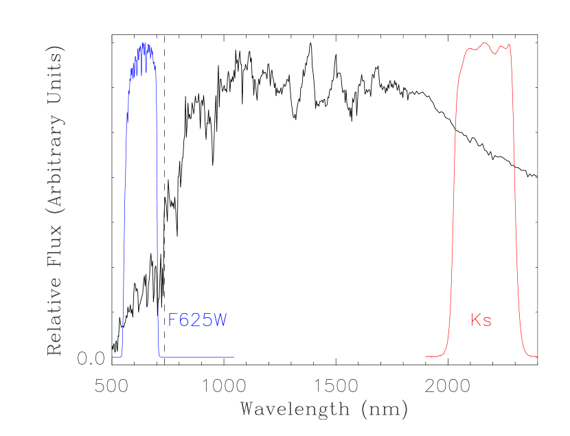
Figure 1.— Band-pass filters used in this work to select red-sequence galaxies. As a reference, a simple stellar population, 12 Gyr old, solar metallicity spectral energy distribution from the Bruzual-Charlot (Bruzual & Charlot, 2003) library, redshifted to the cluster redshift ($z=0.837$), is shown. The chosen filters straddle the rest-frame 4000Å-break (vertical, dashed line) and the $K_{s}$ band provides coverage of the spectrophotometric region dominated by the bulk of the stellar content in early-type galaxies.

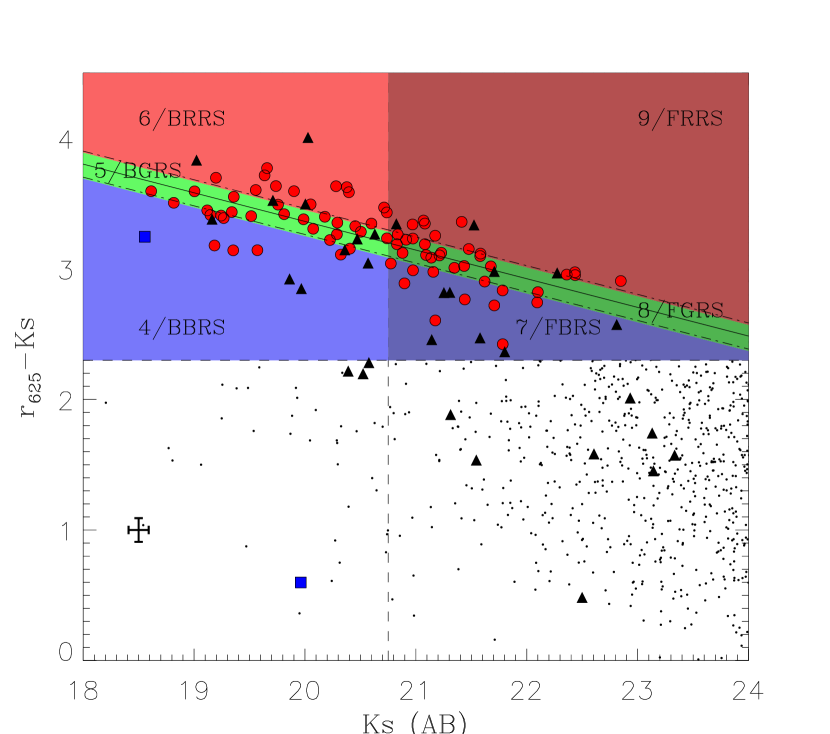
Figure 2.— Definition of regions in color-magnitude space used to stack spectra within the red-sequence (RS). The horizontal dashed line has arbitrarily been set at $r_{625}-Ks=2.3$ to separate blue from red galaxies. We consider galaxies with a $r_{625}-Ks>2.3$ color as galaxies within the cluster RS. The vertical dashed line has arbitrarily been set to $Ks=20.75$ ($\sim K^{*}+1$) to divide the RS into “bright” and “faint” bins. The RS is thus divided into 3 bright and 3 faint regions. The three bright regions, named 4/BBRS, 5/BGRS and 6/BRRS, are defined in table 2. The three faint regions, 7/FBRS, 8/FGRS and 9/FRRS, are also defined in table 2. The fit to the red sequence is indicated by the solid black line, while the dot-dashed black lines are at $\pm 0.1$ in ($r_{625}-Ks$) from the fit. The cross at the lower-left of the plot indicates typical error bars in magnitude and color. Red circles correspond to passive cluster members, black triangles correspond to star-forming members, and the two blue squares are the confirmed AGN members. The black dots are sources within the ACS mosaic for which photometric information is available. Star formation histories within these regions allows us to study variations of the stellar content of cluster galaxies as a function of galaxy color and luminosity.

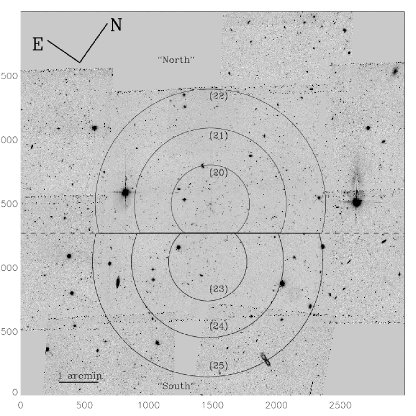
Figure 3.— Regions used to co-add spectra according to the projected angular distribution of the galaxies. Because of the complex structure of RX J0152.7-1357, composed of two central clumps likely in the process of merging, we have defined a set of regions that take into account the existence of both sub-clusters. The cluster field of view is separated in two halves at a fiducial central point, as indicated by the horizontal dashed line. Then we define two groups of concentric (semi-)annuli (solid contours) centered at each clump, however, truncated at the separation half-way between them. Sectors associated with the northern clump (20/N0 through 22/N2) are labeled as “North”, while those associated with the southern clump (23/S0 through 25/S2) are labeled as “South”. The background image corresponds to the ACS 5$\farcm$8 $\times$ 5$\farcm$8 central mosaic, complemented by 7 ACS flanking fields subsequently obtained in V (F606W) and I (F814W).

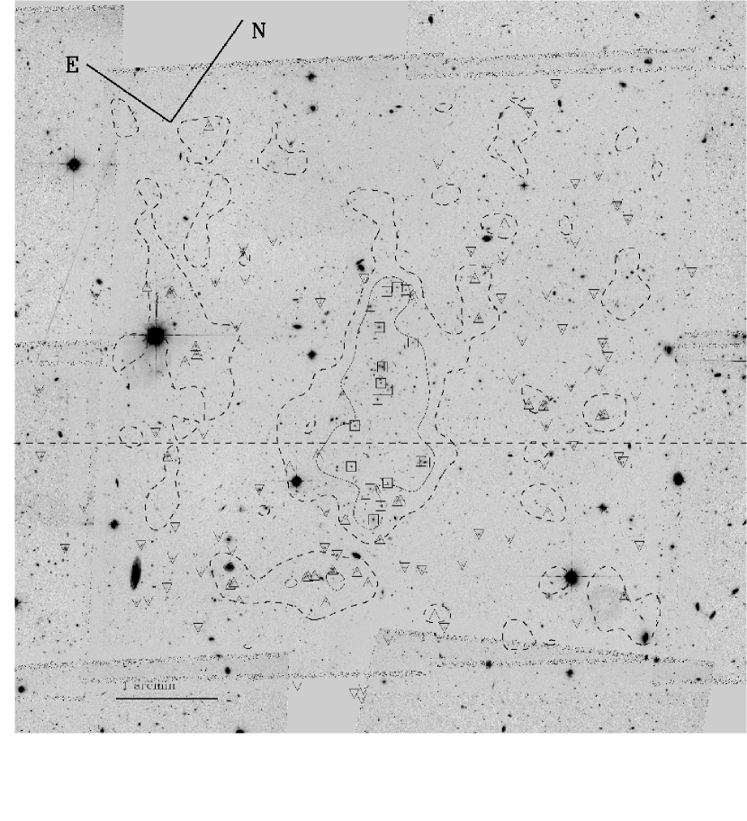
Figure 4.— Mass density environments defined from the $\kappa$ map of RX J0152.7-1357 (Jee et al., 2005). Because of the sheet-mass degeneracy, we use this map in a relative sense only, during the interpretation of the results. The smoothing scale of the map is $\sim 20$″, and its accuracy, about 20%. Three different environments are arbitrarily identified. The first of them is characterized by mass densities $>20\times\sigma_{DM}$ (solid contours), with $\sigma_{DM}=0.0057\times\Sigma_{c}$, being $\Sigma_{c}\sim 3650M_{\odot}\ pc^{-2}$ the critical mass density of the cluster (Blakeslee et al., 2006). The $\kappa$ value around the two brightest central galaxies of the northern clump (the cluster center adopted in Jee et al., 2005) is $\sim$0.3. The second one is that containing mass densities between 5 (dashed contours) and 20 times $\sigma_{DM}$, while the last of the three encompasses mass densities $<5\times\sigma_{DM}$, reaching negative values in some areas. These three environments correspond to regions 17/HDMD, 18/MDMD, and 19/LDMD, respectively, as presented in table 2. The distribution of spectroscopic members is indicated by the symbols. Members in the highest density regions are indicated as squares; members in the intermediate density regions, as triangles; and members in the lowest density environments, as upside-down triangles. For comparison, we also show the horizontal dashed line in Fig. 3 that contains the mid-point between the two main central sub-clusters. The background image shows the ACS data, 7$\farcm$2 a side and centered at the two brightest central galaxies of the northern clump.

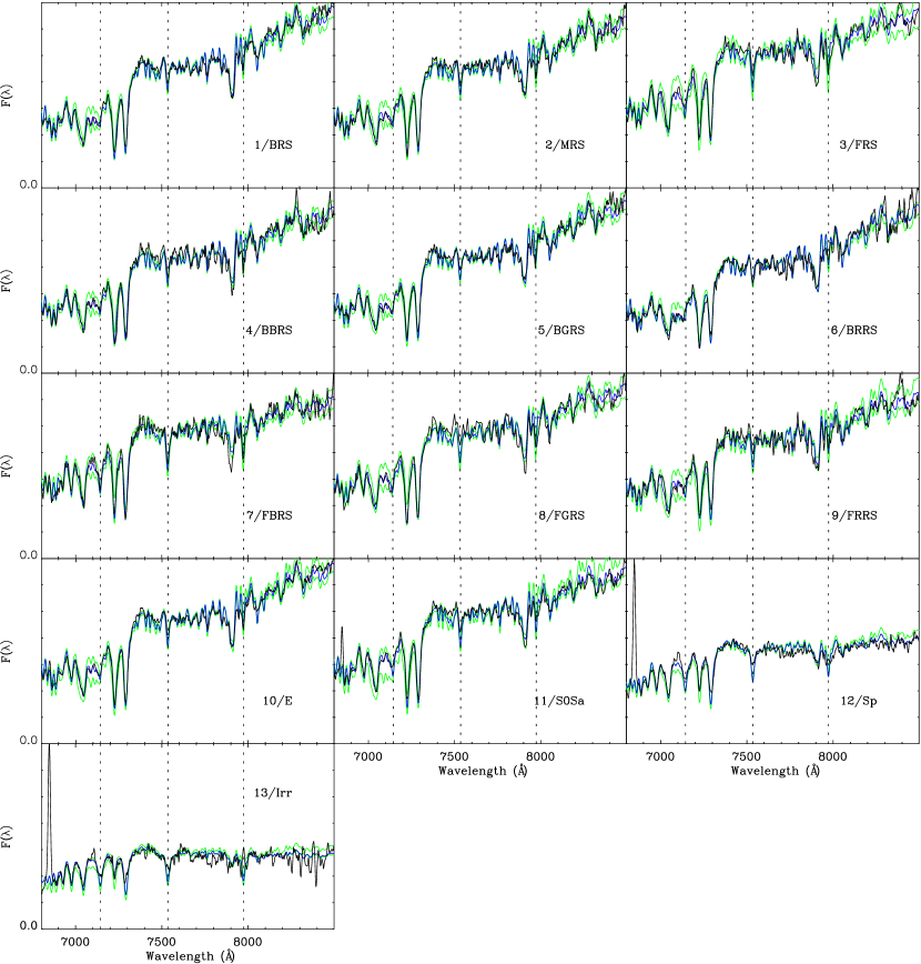
Figure 5.— The resulting stacked spectrum of galaxies for hyperspace regions 1/BRS through 13/Irr (as defined in table 2) is shown as a black line. The “best-fitting” spectrophotometric model (as defined in §3.4) is shown as the blue line, while the minimum and maximum fitting flux values within the intersection of the 99.7% confidence regions (see §3.4), and as a function of wavelength, are represented by the green lines. Relative flux is in arbitrary units and all the spectra are shown redshifted to the mean cluster redshift, $z=0.837$ (Demarco et al., 2005). In order to visualize the correlation between H6 and other Balmer features such as H$\delta$ and H$\gamma$, the vertical dashed lines indicate the location of these features from left to right, respectively.

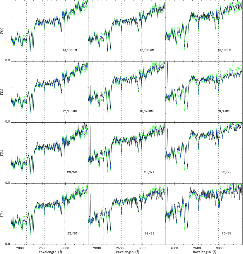
Figure 6.— As in Fig. 5, but here for hyperspace regions 14/RSHM through 25/S2.

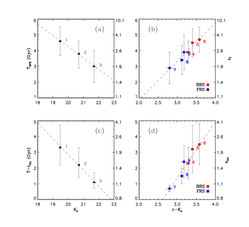
Figure 7.— SFHs for galaxies in the RS as a function of $K_{s}$ brightness and $r_{625}-K_{s}$ color. Results from the three-bin partition (regions 1/BRS through 3/FRS) are shown in panels (a) and (c). Results from the finer RS partition (regions 4/BBRS through 9/FRRS) are shown in panels (b) and (d). For clarity, bins in the bright half of the red-sequence (BRS) and in the faint half of the red-sequence (FRS) are shown in red and blue, respectively. The dashed lines are the best linear fits to the data points considering error bars. On average, galaxies in the brighter and redder RS bins are older and also display shorter periods of active star formation, i.e., longer $T-t_{fin}$ lookback times (see §4.1.1 for details).

Figure 8.— SFHs of passive RS galaxies as a function of average stellar mass, $M_{*,SED}$, for the three mass bins, 14/RSHM, 15/RSMM and 16/RSLM. Average stellar mass is obtained by averaging the individual stellar masses of galaxies in each bin, and the corresponding error bars are calculated as the standard error. The dashed lines represent linear fits to the data taking into account error bars. Lower stellar mass bins tend to have, on average, younger ages and more extended periods of active star formation (see §4.1.2 for details).

Figure 9.— SFHs of cluster galaxies as a function of local projected DM density, $\Sigma_{DM}$, for the three bins, 17/HDMD through 19/LDMD. The dashed lines represent linear fits to the data taking into account error bars. The results are consistent with each other within the errors. On average, the bulk of the stars in cluster galaxies were formed at roughly the same time, $z_{f}\sim 2.6$ which corresponds to a $T_{SFR}\sim 3.8$ Gyr. However, galaxies in the lowest DM density environment (19/LDMD) form stars down to $\sim 0.8$ Gyr prior to the epoch of observation ($z=0.837$), while the average galaxy in the highest density region (17/HDMD) stopped forming stars $\sim 3.2$ Gyr prior to the epoch of observation (see §4.1.3).

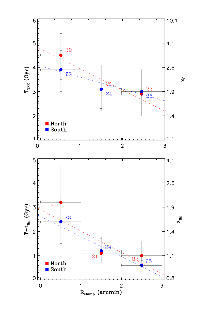
Figure 10.— SFHs of cluster galaxies as a function of radial distance from the center of each of the two main subclusters, as defined in table 2. Red points correspond to regions 20/N0 through 22/N2 in the northern subcluster while blue points correspond to regions 23/S0 through 25/S2 in the southern subcluster. The corresponding linear fits are shown as dashed red and blue lines. Although not statistically significant, there is some indication that the central region of the northern subcluster is slightly older and has stopped forming stars earlier than the central region of the southern subcluster (see §4.1.3).

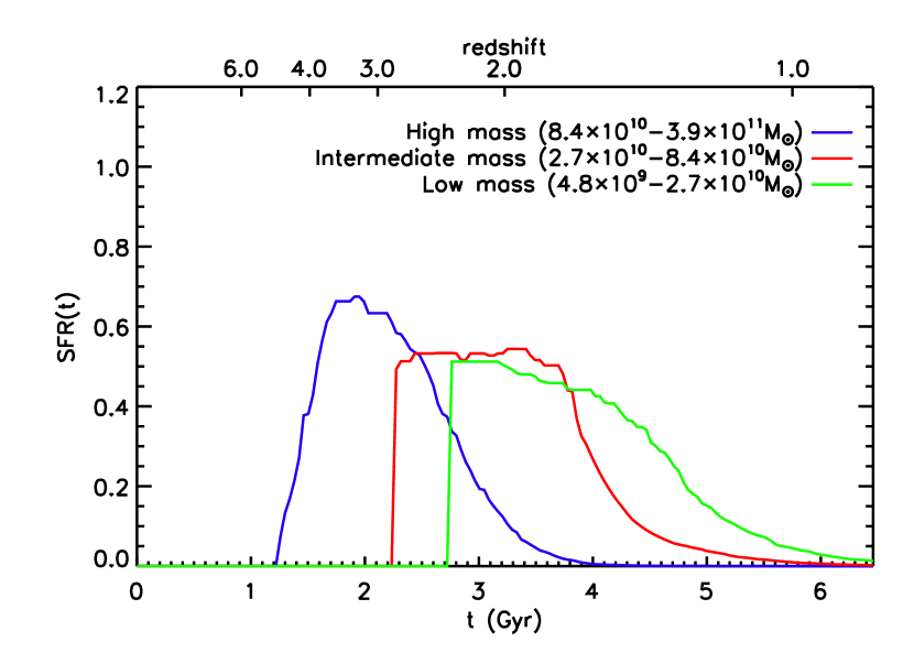
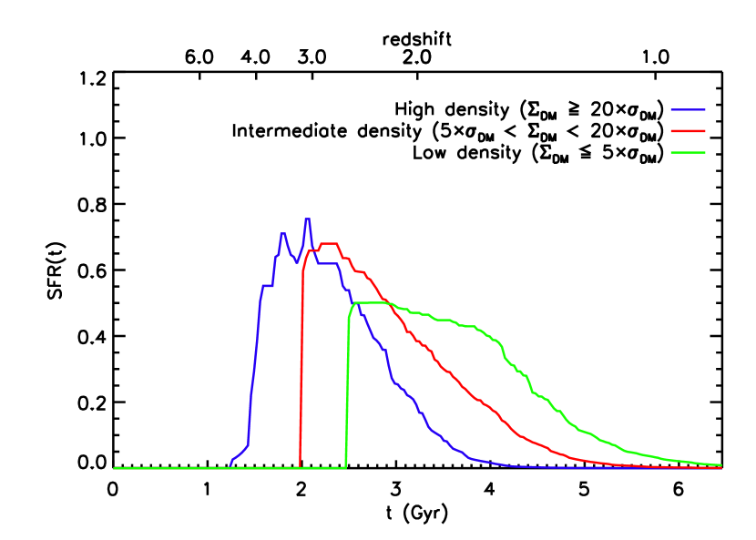
Figure 11.— Median SFHs of the best-fitting models of the spectrophotometric data of non-[O$\mathrm{II}$] galaxies in the stellar mass-selected regions, 14/RSHM through 16/RSLM (left), and local dark matter density regions, 17/HDMD through 19/LDMD (right). The bottom axis shows the cosmic time $t$ and the top axis shows the corresponding redshift. High mass galaxies and those in the highest density environments have formed the bulk of their stars at $z>3$ and stopped their star-forming activity at $z\sim 2$ altogteher, with the most massive galaxies ($>8\times 10^{10}\ M_{\odot}$) being $\sim 1$ Gyr older than the less massive ones ($3\times 10^{10}\ M_{\odot}$). These ages suggest a formation scenario involving an accelerated SFH and early quenching of star formation.

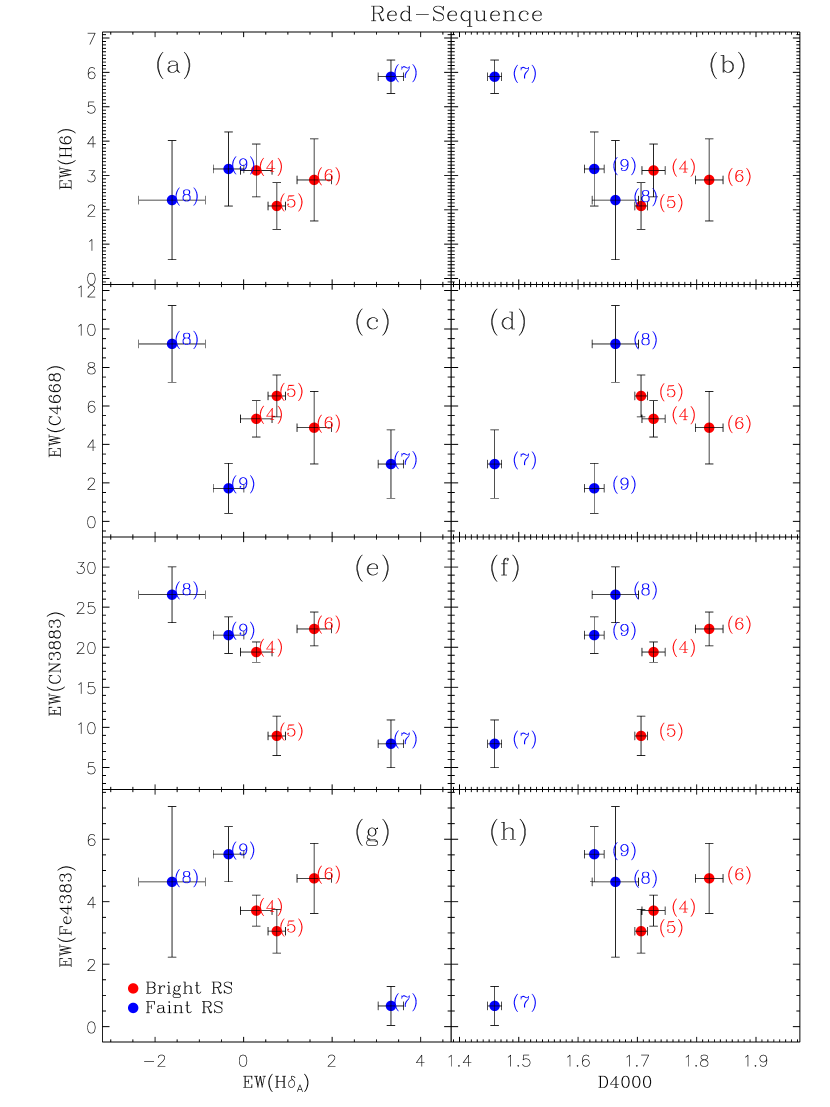
Figure 12.— Distribution of spectral indices for galaxies in the red-sequence. Red circles correspond to regions in the bright half of the RS while blue circles correspond to regions in the faint half. Only passive galaxies, i.e., galaxies with no detectable [O$\mathrm{II}$] in emission, have been stacked in each region. In general, notable deviations ($>2\sigma$) of region 7/FBRS with respect to the brightest and reddest region (6/BRRS) in the red-sequence can be seen for most of the indices shown.

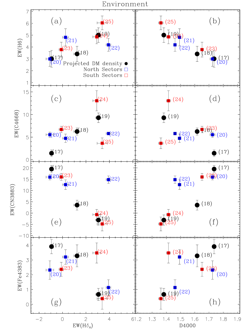
Figure 13.— Distribution of spectral indices for galaxies grouped according to local environment. The latter is characterized in three different ways: projected DM density (black circles), angular distribution in the northern subcluster (blue squares), and angular distribution in the southern subcluster (red squares), as defined in §3.2 (see table 2). All (passive and star-forming, but no AGN) galaxies have been stacked in each region. Clear trends of the age-sensitive indices with environment are observed. H$\delta_{A}$ and H6 increase, on average, toward the outskirts of the subclusters and with decreasing projected DM density, while the opposite trend is observed for the D4000 index. As opposed to the EW(C4668), the EW(CN3883) and EW(Fe4383) show a notable decrease toward lower DM density regions. Gradients with radial distance are only notable for the CN3883 and Fe4383 indices depending on the substructure.

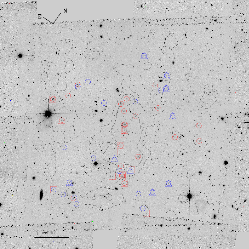
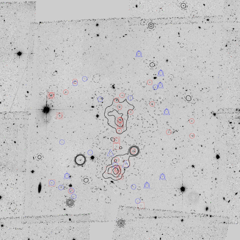
Figure 14.— Angular distribution of passive cluster members. The background image in each panel shows the same ACS data, 7$\farcm$2 a side and centered at the two brightest central galaxies of the northern clump, as in Fig. 4. The left panel shows the same dark matter density contours of Fig. 4. The right panel shows X-ray Chandra contours (see Demarco et al., 2005). The dashed contour indicates the 3-$\sigma$ level and the solid contours are the 10, 20 and 30-$\sigma$ levels. The color symbols are the same for both panels. Red squares and blue triangles correspond to red-sequence passive members in regions 6/BRRS and 7/FBRS, respectively. The circles correspond to RS passive members grouped by stellar mass: red, white and blue symbols are galaxies within regions 14/RSHM, 15/RSMM and 16/RSLM, respectively, as defined in table 2. Clearly, less massive galaxies prefer lower density environment in the same way as the faintest and bluest galaxies in the red-sequence do.

References

- Appenzeller & Rupprecht (1992) Appenzeller, I., & Rupprecht, G. 1992, The ESO Messenger, March, 18
- Avni (1976) Avni, Y. 1976, ApJ, 210, 642
- Balogh et al. (1999) Balogh, M. L., Morris, S. L., Yee, H. K. C., Carlberg, R. G., & Ellingson, E. 1999, ApJ, 527, 54
- Bekki et al. (2002) Bekki, K., Couch, W. J., & Shioya, Y. 2002, ApJ, 577, 651
- Bell et al. (2003) Bell, E. F., McIntosh, D. H., Katz, N., & Weinberg, M. D. 2003, ApJS, 149, 289
- Bell et al. (2006) Bell, E. F., et al. 2006, ApJ, 640, 241
- Bernardi et al. (2006) Bernardi, M., Nichol, R. C., Sheth, R. K., Miller, C. J., & Brinkmann, J. 2006, AJ, 131, 1288
- Bertin & Arnouts (1996) Bertin, E., & Arnouts, S. 1996, A&AS, 117, 393
- Blakeslee et al. (2003a) Blakeslee, J. P., Anderson, K. R., Meurer, G. R., Benítez, N., & Magee, D. 2003, Astronomical Data Analysis Software and Systems XII, 295, 257
- Blakeslee et al. (2003b) Blakeslee, J. P., et al. 2003, ApJ, 596, L143
- Blakeslee et al. (2006) Blakeslee, J. P., et al. 2006, ApJ, 644, 30
- Braglia et al. (2009) Braglia, F. G., Pierini, D., Biviano, A., & Boehringer, H. 2009, A&A, 500, 947
- Bruzual A. (1983) Bruzual A., G. 1983, ApJ, 273, 105
- Bruzual & Charlot (2003) Bruzual, G., & Charlot, S. 2003, MNRAS, 344, 1000
- Bundy et al. (2006) Bundy, K., et al. 2006, ApJ, 651, 120
- Calzetti et al. (2000) Calzetti, D., Armus, L., Bohlin, R. C., Kinney, A. L., Koornneef, J., & Storchi-Bergmann, T. 2000, ApJ, 533, 682
- Cimatti et al. (2006) Cimatti, A., Daddi, E., & Renzini, A. 2006, A&A, 453, L29
- Collins et al. (2009) Collins, C. A., et al. 2009, Nature, 458, 603
- Cooper et al. (2007) Cooper, M. C., et al. 2007, MNRAS, 376, 1445
- Couch & Sharples (1987) Couch, W. J., & Sharples, R. M. 1987, MNRAS, 229, 423
- Cowie et al. (1996) Cowie, L. L., Songaila, A., Hu, E. M., & Cohen, J. G. 1996, AJ, 112, 839
- Davidge & Clark (1994) Davidge, T. J., & Clark, C. C. 1994, AJ, 107, 946
- Della Ceca et al. (2000) Della Ceca, R., Scaramella, R., Gioia, I. M., Rosati, P., Fiore, F., & Squires, G. 2000, A&A, 353, 498
- De Lucia et al. (2007) De Lucia, G., et al. 2007, MNRAS, 374, 809
- Demarco et al. (2005) Demarco, R., et al. 2005, A&A, 432, 381
- Demarco et al. (2007) Demarco, R., et al. 2007, ApJ, 663, 164
- de Vaucouleurs (1961) de Vaucouleurs, G. 1961, ApJS, 5, 233
- de Vaucouleurs et al. (1976) de Vaucouleurs, G., de Vaucouleurs, A., & Corwin, H. G. 1976, University of Texas Monographs in Astronomy (Austin: Univ. Texas Press)
- Doherty et al. (2006) Doherty, M., Bunker, A., Sharp, R., Dalton, G., Parry, I., & Lewis, I. 2006, MNRAS, 370, 331
- Dressler (1980) Dressler, A. 1980, ApJ, 236, 351
- Dressler et al. (1999) Dressler, A., Smail, I., Poggianti, B. M., Butcher, H., Couch, W. J., Ellis, R. S., & Oemler, A. J. 1999, ApJS, 122, 51
- Dressler et al. (2004) Dressler, A., Oemler, A. J., Poggianti, B. M., Smail, I., Trager, S., Shectman, S. A., Couch, W. J., & Ellis, R. S. 2004, ApJ, 617, 867
- Ellis & Jones (2004) Ellis, S. C., & Jones, L. R. 2004, MNRAS, 348, 165
- Emerson (1999) Emerson, D. 1999, Interpreting Astronomical Spectra, by D. Emerson, pp. 472. ISBN 0-471-97679-2. Wiley-VCH , March 1999
- Faber et al. (2007) Faber, S. M., et al. 2007, ApJ, 665, 265
- Ford et al. (1998) Ford, H. C., et al. 1998, Proc. SPIE, 3356, 234
- Ford et al. (2004) Ford, H., et al. 2004, Penetrating Bars Through Masks of Cosmic Dust, 319, 459
- Gallazzi et al. (2006) Gallazzi, A., Charlot, S., Brinchmann, J., & White, S. D. M. 2006, MNRAS, 370, 1106
- Girardi et al. (2000) Girardi, L., Bressan, A., Bertelli, G., & Chiosi, C. 2000, A&AS, 141, 371
- Girardi et al. (2005) Girardi, M., Demarco, R., Rosati, P., & Borgani, S. 2005, A&A, 442, 29
- Gobat et al. (2008) Gobat, R., Rosati, P., Strazzullo, V., Rettura, A., Demarco, R., & Nonino, M. 2008, A&A, 488, 853
- Gobat (2009) Gobat, R. 2009, Ph.D. Thesis, Ludwig-Maximilians-Universität, Munich
- Gray et al. (2004) Gray, M. E., Wolf, C., Meisenheimer, K., Taylor, A., Dye, S., Borch, A., & Kleinheinrich, M. 2004, MNRAS, 347, L73
- Hilton et al. (2009) Hilton, M., et al. 2009, ApJ, 697, 436
- Holden et al. (2004) Holden, B. P., Stanford, S. A., Eisenhardt, P., & Dickinson, M. 2004, AJ, 127, 2484
- Holden et al. (2007) Holden, B. P., et al. 2007, ApJ, 670, 190
- Homeier et al. (2005) Homeier, N. L., et al. 2005, ApJ, 621, 651
- Jee et al. (2005) Jee, M. J., White, R. L., Benítez, N., Ford, H. C., Blakeslee, J. P., Rosati, P., Demarco, R., & Illingworth, G. D. 2005, ApJ, 618, 46
- Jørgensen et al. (2005) Jørgensen, I., Bergmann, M., Davies, R., Barr, J., Takamiya, M., & Crampton, D. 2005, AJ, 129, 1249
- Joy et al. (2001) Joy, M., et al. 2001, ApJ, 551, L1
- Kauffmann et al. (2003) Kauffmann, G., et al. 2003, MNRAS, 341, 33
- Kawata & Mulchaey (2008) Kawata, D., & Mulchaey, J. S. 2008, ApJ, 672, L103
- Kelson et al. (2006) Kelson, D. D., Illingworth, G. D., Franx, M., & van Dokkum, P. G. 2006, ApJ, 653, 159
- Kennicutt (1998) Kennicutt, R. C., Jr. 1998, ARA&A, 36, 189
- Kinney et al. (1996) Kinney, A. L., Calzetti, D., Bohlin, R. C., McQuade, K., Storchi-Bergmann, T., & Schmitt, H. R. 1996, ApJ, 467, 38
- Kodama & Arimoto (1997) Kodama, T., & Arimoto, N. 1997, A&A, 320, 41
- Kodama et al. (2007) Kodama, T., Tanaka, I., Kajisawa, M., Kurk, J., Venemans, B., De Breuck, C., Vernet, J., & Lidman, C. 2007, MNRAS, 377, 1717
- Kuntschner (2000) Kuntschner, H. 2000, MNRAS, 315, 184
- Kurtz et al. (1992) Kurtz, M. J., Mink, D. J., Wyatt, W. F., Fabricant, D. G., Torres, G., Kriss, G. A., & Tonry, J. L. 1992, Astronomical Data Analysis Software and Systems I, 25, 432
- Larson et al. (1980) Larson, R. B., Tinsley, B. M., & Caldwell, C. N. 1980, ApJ, 237, 692
- Lemaux et al. (2010) Lemaux, B. c., Lubin, L. M., Shapley, A., Kocevski, D., Gal, R. R., & Squires, G. K. 2010, ApJ, 716, 970
- Lidman et al. (2004) Lidman, C., Rosati, P., Demarco, R., Nonino, M., Mainieri, V., Stanford, S. A., & Toft, S. 2004, A&A, 416, 829
- Lidman et al. (2008) Lidman, C., et al. 2008, A&A, 489, 981
- Lin et al. (2008) Lin, L., et al. 2008, ApJ, 681, 232
- Maraston et al. (2003) Maraston, C., Greggio, L., Renzini, A., Ortolani, S., Saglia, R. P., Puzia, T. H., & Kissler-Patig, M. 2003, A&A, 400, 823
- Maraston (2005) Maraston, C. 2005, MNRAS, 362, 799
- Marcillac et al. (2007) Marcillac, D., Rigby, J. R., Rieke, G. H., & Kelly, D. M. 2007, ApJ, 654, 825
- Maughan et al. (2003) Maughan, B. J., Jones, L. R., Ebeling, H., Perlman, E., Rosati, P., Frye, C., & Mullis, C. R. 2003, ApJ, 587, 589
- Mei et al. (2006a) Mei, S., et al. 2006a, ApJ, 639, 81
- Mei et al. (2006b) Mei, S., et al. 2006b, ApJ, 644, 759
- Moore et al. (1998) Moore, B., Lake, G., & Katz, N. 1998, ApJ, 495, 139
- Moorwood et al. (1998) Moorwood, A., Cuby, J.-G., & Lidman, C. 1998, ESO Messenger, 91, 9
- Oke (1974) Oke, J. B. 1974, ApJS, 27, 21
- Papovich et al. (2010) Papovich, C., et al. 2010, ApJ, 716, 1503
- Patel et al. (2009) Patel, S. G., Kelson, D. D., Holden, B. P., Illingworth, G. D., Franx, M., van der Wel, A., & Ford, H. 2009, ApJ, 694, 1349
- Poggianti & Barbaro (1997) Poggianti, B. M., & Barbaro, G. 1997, A&A, 325, 1025
- Poggianti et al. (1999) Poggianti, B. M., Smail, I., Dressler, A., Couch, W. J., Barger, A. J., Butcher, H., Ellis, R. S., & Oemler, A. J. 1999, ApJ, 518, 576
- Postman et al. (2005) Postman, M., et al. 2005, ApJ, 623, 721
- Press et al. (1992) Press, W. H., Teukolsky, S. A., Vetterling, W. T., & Flannery, B. P. 1992, Cambridge: University Press, —c1992, 2nd ed.,
- Prochaska et al. (2007) Prochaska, L. C., Rose, J. A., Caldwell, N., Castilho, B. V., Concannon, K., Harding, P., Morrison, H., & Schiavon, R. P. 2007, AJ, 134, 321
- Rettura et al. (2006) Rettura, A., et al. 2006, A&A, 458, 717
- Rettura et al. (2010) Rettura, A., et al. 2010, ApJ, 709, 512
- Rieke et al. (2004) Rieke, G. H., et al. 2004, ApJS, 154, 25
- Rosati et al. (1998) Rosati, P., della Ceca, R., Norman, C., & Giacconi, R. 1998, ApJ, 492, L21
- Salpeter (1955) Salpeter, E. E. 1955, ApJ, 121, 161
- Sarazin (1988) Sarazin, C. L. 1988, Cambridge Astrophysics Series, Cambridge: Cambridge University Press, 1988
- Schlegel et al. (1998) Schlegel, D. J., Finkbeiner, D. P., & Davis, M. 1998, ApJ, 500, 525
- Smail et al. (1999) Smail, I., Morrison, G., Gray, M. E., Owen, F. N., Ivison, R. J., Kneib, J.-P., & Ellis, R. S. 1999, ApJ, 525, 609
- Smith et al. (2005) Smith, G. P., Treu, T., Ellis, R. S., Moran, S. M., & Dressler, A. 2005, ApJ, 620, 78
- Stanford et al. (1998) Stanford, S. A., Eisenhardt, P. R., & Dickinson, M. 1998, ApJ, 492, 461
- Stott et al. (2007) Stott, J. P., Smail, I., Edge, A. C., Ebeling, H., Smith, G. P., Kneib, J.-P., & Pimbblet, K. A. 2007, ApJ, 661, 95
- Swinbank et al. (2005) Swinbank, A. M., Balogh, M. L., Bower, R. G., Hau, G. K. T., Allington-Smith, J. R., Nichol, R. C., & Miller, C. J. 2005, ApJ, 622, 260
- Tanaka et al. (2005) Tanaka, M., Kodama, T., Arimoto, N., Okamura, S., Umetsu, K., Shimasaku, K., Tanaka, I., & Yamada, T. 2005, MNRAS, 362, 268
- Tanaka et al. (2006) Tanaka, M., Kodama, T., Arimoto, N., & Tanaka, I. 2006, MNRAS, 365, 1392
- Tanaka et al. (2008) Tanaka, M., et al. 2008, A&A, 489, 571
- Thomas et al. (2003) Thomas, D., Maraston, C., & Bender, R. 2003, MNRAS, 339, 897
- Thomas et al. (2004) Thomas, D., Maraston, C., & Korn, A. 2004, MNRAS, 351, L19
- Thomas et al. (2005) Thomas, D., Maraston, C., Bender, R., & Mendes de Oliveira, C. 2005, ApJ, 621, 673
- Tonry & Davis (1979) Tonry, J., & Davis, M. 1979, AJ, 84, 1511
- Tran et al. (2003) Tran, K.-V. H., Franx, M., Illingworth, G., Kelson, D. D., & van Dokkum, P. 2003, ApJ, 599, 865
- Tran et al. (2005) Tran, K.-V. H., van Dokkum, P., Franx, M., Illingworth, G. D., Kelson, D. D., & Schreiber, N. M. F. 2005, ApJ, 627, L25
- Tran et al. (2007) Tran, K.-V. H., Franx, M., Illingworth, G. D., van Dokkum, P., Kelson, D. D., Blakeslee, J. P., & Postman, M. 2007, ApJ, 661, 750
- Tremonti et al. (2004) Tremonti, C. A., et al. 2004, ApJ, 613, 898
- Treu et al. (2003) Treu, T., Ellis, R. S., Kneib, J.-P., Dressler, A., Smail, I., Czoske, O., Oemler, A., & Natarajan, P. 2003, ApJ, 591, 53
- van der Wel et al. (2007) van der Wel, A., et al. 2007, ApJ, 670, 206
- van Dokkum et al. (1999) van Dokkum, P. G., Franx, M., Fabricant, D., Kelson, D. D., & Illingworth, G. D. 1999, ApJ, 520, L95
- van Dokkum & Stanford (2003) van Dokkum, P. G., & Stanford, S. A. 2003, ApJ, 585, 78
- van Dokkum (2005) van Dokkum, P. G. 2005, AJ, 130, 2647
- Visvanathan & Sandage (1977) Visvanathan, N., & Sandage, A. 1977, ApJ, 216, 214
- Wolf et al. (2005) Wolf, C., Gray, M. E., & Meisenheimer, K. 2005, A&A, 443, 435
- Worthey et al. (1994) Worthey, G., Faber, S. M., Gonzalez, J. J., & Burstein, D. 1994, ApJS, 94, 687
- Worthey et al. (1995) Worthey, G., Trager, S. C., & Faber, S. M. 1995, Fresh Views of Elliptical Galaxies, 86, 203
- Worthey & Ottaviani (1997) Worthey, G., & Ottaviani, D. L. 1997, ApJS, 111, 377
- Zabludoff & Mulchaey (1998) Zabludoff, A. I., & Mulchaey, J. S. 1998, ApJ, 496, 39