Mixed-Morphology Supernova Remnants in X-rays: Isothermal Plasma in HB21 and Probable Oxygen-Rich Ejecta in CTB 1

Abstract

We present an analysis of X-ray observations of the Galactic supernova remnants (SNRs) HB21 (G89.0$+$4.7) and CTB 1 (G116.9$+$0.2), two well-known members of the class of mixed-morphology (MM) SNRs. Our analysis draws upon observations of both SNRs made with the Advanced Satellite for Cosmology and Astrophysics (ASCA): we have also used an archived Chandra observation of CTB 1 as part of this effort. We find a marked contrast between the X-ray properties of HB21 and CTB 1: in the case of HB21, the extracted spectra of the northwest and southeast regions of the X-ray emitting plasma associated with the SNR can be fit with a single thermal model with marginally enhanced silicon and sulfur abundances. For both of these regions, the derived column density and temperature are $N$_H $\sim$ 0.3$\times$10²² cm^-2 and $\it{kT}$ $\sim$ 0.7 keV, respectively. No significant spatial differences in temperature or elemental abundances between the two regions are detected and the X-ray-emitting plasma for both regions is close to ionization equilibrium. Our Chandra spectral analysis of CTB 1 reveals that this source is likely an oxygen-rich SNR with enhanced abundances of oxygen and neon: this result is quite surprising for an evolved SNR like CTB 1. The high angular resolution Chandra observation of CTB 1 reveals spectral variations across this SNR: in particular, we have detected localized hard emission with an angular extent of $\sim 1^{\prime}$. The extracted ASCA spectra for both the southwest and northeastern regions of CTB 1 cannot be fit with a single thermal component and instead an additional component is required to account for the presence of excess emission seen at higher energies. Based on our fits to the extracted ASCA spectra, we derive a column density $N$_H $\sim$ 0.6$\times$ 10²² cm^-2 and a temperature for the soft thermal component of $\it{kT}$_soft$\sim$ 0.28 keV for both regions. The hard emission from the southwest region may be modeled with either a thermal component with a temperature $\it{kT}$_hard $\sim$ 3 keV or by a power law component with a photon index $\Gamma$ $\sim$ 2-3; for the northeast region the hard emission may be modeled with a power law component with a photon index $\Gamma$ = 1.4. The detection of center-filled ejecta-dominated X-ray emission from HB21 and CTB 1 as well as other MM SNRs suggests a new scenario for the origin of contrasting X-ray and radio morphologies of this class of sources. Lastly, we have analyzed the properties of the discrete hard X-ray source 1WGA J0001.4$+$6229 which is seen in projection just inside the northeastern shell of CTB 1. Our extracted ASCA GIS spectra of this source are best fit using a power-law model with a photon index $\Gamma$=2.2${}^{+0.5}_{-1.2}$: this slope is typical for featureless power-law continua produced by rotation-powered pulsars. This source may be a neutron star associated with CTB 1. We find marginal evidence for X-ray pulsations from this source with a period of 47.6154 milliseconds. A deep radio observation of this source failed to reveal any pulsations.

1 Introduction

A new morphological class of supernova remnants (SNRs) known as the mixed-morphology (MM) SNRs has been firmly established in the recent literature (Rho & Petre, 1998; Shelton et al., 1999). The defining characteristics of SNRs of this class include a shell-like radio morphology combined with a centrally-filled X-ray morphology. X-ray observations of these SNRs made with the $\it{Roentgensatellit}$ (ROSAT), the Advanced Satellite for Cosmology and Astrophysics (ASCA), Chandra and XMM-Newton have found that the central X-ray emission from these SNRs is not non-thermal emission (as would be expected from a central plerion) but instead thermal from shock-heated swept-up interstellar material. Examples of well-known MM SNRs include W28 (Rho & Borkowski, 2002), G290.1$-$0.8 (MSH 11$-$6$\it{1}$A) (Slane et al., 2002) and IC 443 (Kawasaki et al., 2002). Rho & Petre (1998) suggested that as many as 25% of the entire population of Galactic SNRs may belong to this morphological class. Based on CO and infrared observations (Koo et al., 2001; Reach et al., 2005), it appears that many MM SNRs are interacting with nearby molecular and HI clouds. This result suggests a connection between the contrasting X-ray and radio morphologies of these SNRs with the interaction between these sources and adjacent clouds, but such a connection lacks a detailed theoretical basis at this time. Two leading scenarios have been advanced to explain the origin of the contrasting radio and X-ray morphologies of MM SNRs: in the first scenario – known as the evaporating clouds scenario – molecular clouds overrun by the expanding shock front of the SNR survive passage through the shock and eventually evaporate, providing a source of material that increases the density of the interior X-ray-emitting plasma of the SNR (Cowie & McKee, 1977; White & Long, 1991). In the second scenario – known as the radiative shell model – the SNR has evolved to an advanced stage where the shock temperature is low and very soft X-ray emission from the shell is absorbed by the interstellar medium (ISM): therefore, the only detectable X-ray emission is from the interior of the SNR (Cox et al., 1999; Shelton et al., 1999, 2004). In the current paper we analyze and discuss X-ray emission from two Galactic SNRs – HB21 and CTB 1 – which have both been previously classified as MM SNRs by Rho & Petre (1998).

HB21 (G89.0$+$4.7) was discovered in a radio survey by Brown & Hazard (1953). The radio angular extent of this SNR is large – 120$\times$90 arcminutes (Green, 2009a) – and the radio morphology is a closed shell. The shell appears to be flattened along the eastern boundary and features bright regions along the northern and southern boundaries with a prominent indentation seen along the northern boundary. The radio emission from HB21 is strongly polarized (3.7$\%$$\pm$0.4$\%$) with a projected magnetic field tangential to the shell (Kundu, 1971; Kundu et al., 1973; Kothes et al., 2006), suggesting that the shell was compressed during the radiative evolutionary stage of the SNR. The measured radio spectral index for this SNR is $\alpha$ $\sim$ 0.4 ($S_{\nu}\propto\nu^{-\alpha}$) (Leahy, 2006; Green, 2009b) but significant variations in the values (from 0.0-0.8 with a standard deviation of 0.16) of the spectral index across the face of the SNR were observed by Leahy (2006). Based on IRAS observations, Saken et al. (1992) detected clumpy infrared filaments associated with this SNR. Filamentary optical emission from this SNR with an angular extent comparable to the radio shell was detected by Mavromatakis et al. (2007). Extensive evidence exists that indicates HB21 is interacting with adjacent molecular clouds: this evidence includes CO observations (Tatematsu et al., 1990; Koo et al., 2001; Byun et al., 2006) as well as near- and mid-infrared observations of the sites of shock-molecular cloud interactions along the northern and southern parts of the SNR (Shinn et al., 2009, 2010). HI observations toward HB21 (Tatematsu et al., 1990; Koo & Heiles, 1991) have revealed a high velocity expanding shell associated with this SNR. Finally, HB21 has been the subject of prior pointed X-ray observations made by Einstein (Leahy, 1987) and ROSAT (Rho, 1995; Leahy & Aschenbach, 1996): we include in this paper the ROSAT images presented previously by Rho (1995) in her PhD thesis work. No pulsars or $\gamma$-ray sources are believed to be associated with HB21: radio searches for a pulsar associated with this SNR were conducted by Biggs & Lyne (1996) and Lorimer et al. (1998) but no candidate sources were found. The distance to HB21 is not well known: Tatematsu et al. (1990) argued for a distance of only 0.8 kpc based on an association between the SNR and molecular material that belongs to the Cygnus OB7 association (Humphreys, 1978). However, Yoshita et al. (2001) suggested a distance of $\geq$1.6 kpc based on a correlation that those authors found between X-ray absorbing column density and extinction, and Byun et al. (2006) suggested a distance of 1.7 kpc based on CO observations. In this paper, we have adopted a distance of 1.7 kpc to HB21.

CTB 1 (G116.9$+$0.2) was discovered in a survey of Galactic radio emission at 960 MHz by Wilson & Bolton (1960). Subsequent radio observations of this SNR (Velusamy & Kundu, 1974; Angerhofer et al., 1977; Landecker et al., 1982; Yar-Uyaniker et al., 2004; Tian & Leahy, 2006; Kothes et al., 2006) reveal a radio morphology that may be described as a nearly complete circular shell with a diameter of approximately 34 arcminutes (Green, 2009b). The radio emission is brightest along the western rim and a prominent gap is seen along the northern and northeastern sector of the circular emission. Like HB21, the magnetic field is aligned in the tangential direction, also suggesting that the shell was compressed during the radiative stage of the evolution of the SNR, but compared to HB21 the degree of polarization is much lower (0.4%$\pm$0.1% – see Kothes et al. (2006)). The measured spectral index of the observed radio emission is $\alpha$ $\sim$ 0.6 (Landecker et al., 1982; Kothes et al., 2006; Tian & Leahy, 2006; Green, 2009b). CTB 1 has also been detected at optical wavelengths, in emission lines such as [ OIII ] $\lambda$5007 and [ SII ] $\lambda\lambda$ 6716, 6731; the observed optical shell-like morphology closely matches the radio shell. The optical images of CTB 1 presented by Fesen et al. (1997) depict a remarkable contrast in the emission-line properties of this SNR: while [ SII ] emission is seen from roughly the entire optical shell (with the greatest amount of emission in the south), the [ OIII ] emission appears to be almost entirely localized to the western rim of the shell. Saken et al. (1992) detected infrared emission from CTB 1 in the 60 $\mu$m and 100 $\mu$m IRAS bands: an arc of infrared emission was seen in the 60 $\mu$m/100 $\mu$m ratio image that appears to be coincident with the radio shell. CTB 1 was observed in X-rays with ROSAT (Hailey & Craig, 1995; Rho, 1995; Craig et al., 1997): like other MM SNRs, the X-ray emission from this SNR (which has a thermal origin) lies interior to the radio and optical shells. Remarkably, the X-ray emission is also seen to extend through the known northern gap of the SNR. Like HB21, no pulsars or $\gamma$-ray sources are believed to be associated with CTB 1: a radio search conducted by Lorimer et al. (1998) for a pulsar revealed no candidate sources. Published distance estimates for this SNR have ranged from 1.6 to 3.5 kpc; in this paper we have adopted a distance to CTB 1 of 3.1$\pm$0.4 kpc as measured by Hailey & Craig (1994).

The organization of this paper is as follows: in Section 2 we describe the ASCA X-ray observations of HB21 and CTB 1 and the Chandra observations of CTB 1, including details of data reduction. ROSAT and radio observations of these SNRs are also described in this section. In Section 3 we present the results of our spectral analyses for both HB21 and CTB 1 (in Section 3.1 and Section 3.2, respectively). In Section 4 we discuss the nature of the hard discrete X-ray source 1WGA J0001.4$+$6229: we have discovered weak evidence for pulsed X-ray emission from this source (which is seen in projection against CTB 1) and consider the possibility that it is a neutron star associated with CTB 1. We also present a search for radio pulsations from 1WGA J0001.4$+$6229. Interpretations of our X-ray results for HB21 and CTB 1 are presented in Section 5 and Section 6, respectively. We also detected hard X-ray emission from CTB 1: we discuss the nature of this emission in Section 7. Our preliminary results of this paper have been presented in Pannuti & Rho (2004) after which we note that similiar data sets were analyzed and presented by Lazendic & Slane (2006). Our primary results of HB21 are in agreement with and strengthen those of Lazendic & Slane (2006); for CTB 1, our paper presents extensive and thorough analysis of the Chandra and ASCA data in smaller-scale regions. We also report important new results for this SNR, including the probable detection of oxygen-rich ejecta from CTB 1 as well as spectral variations across the object. In addition, an X-ray hard point-like source is identified and an analysis of its X-ray and radio properties is presented. Finally, the conclusions of this work are summarized in Section 8.

2 Observations and Data Reduction

2.1 ASCA Observations of HB21 and CTB 1

Because the X-ray emission from both HB21 and CTB 1 cover a large angular extent on the sky, two pointed observations were made of each SNR with ASCA (Tanaka et al., 1994), namely the southeast and northwest regions of HB21 and the southwest and northeast regions of CTB 1 (see Table 1 for details of these observations). These observations provided almost a complete spatial coverage of the X-ray emitting gas in both SNRs. The data reduction was conducted using the “XSELECT” program (Version 2.2), which is available from the High Energy Astrophysics Science Archive Research Center (HEASARC). There were two types of instruments onboard ASCA – the Gas Imaging Spectrometer (GIS) and the Solid-State Imaging Spectrometer (SIS) – and both of these instruments were composed of two units denoted as GIS2, GIS3, SIS0 and SIS1, respectively. A single GIS unit sampled a field of view $\sim 50^{\prime}$ in diameter and a background count rate of the GIS is 5 $\times$ 10^-4 counts cm^-2 sec^-1 keV^-1; in comparison, a single SIS unit sampled a field of view approximately $44^{\prime}\times 44^{\prime}$ in size. The nominal FWHM angular resolution of both the GIS and SIS units were approximately 1 arcminute. The standard REV2 screening criteria were applied when reducing both the raw GIS and SIS datasets. We used “FMOSAIC” from the FTOOLS software package to generate an X-ray map by combining the GIS2 and GIS3 maps. We used the FTOOL “MKGISBGD” to prepare blank-sky background spectra and images for each extracted GIS source spectra: for these background datasets, point sources which are brighter than approximately 10^-13 ergs cm^-2 sec^-1 have been removed. Similarly, background spectra were generated using standard SIS blank-sky datasets for analyzing the extracted SIS source spectra. The standard GIS2 and GIS3 response matrix files (RMFs) were used for analyzing extracted the GIS source spectra while the FTOOL “sisrmg” was used to prepare RMFs for the extracted SIS source spectra. Finally, the FTOOL “ASCAARF” was used to prepare ancillary response files (ARFs) for each extracted GIS and SIS source spectra.

2.2 Chandra Observation of CTB 1

We have also analyzed an archival dataset from an additional X-ray observation of CTB 1 made with Chandra (Weisskopf et al., 2002). The corresponding ObsID of this observation is 2810 (PI: S. Kulkarni) and it was conducted as part of a search for central X-ray sources associated with Galactic SNRs. This observation was conducted in FAINT Mode on 14 September 2002 with the Advanced CCD Imaging Spectrometer (ACIS) at a focal plane temperature of $-$120^∘C such that the ACIS-I array of chips sampled a significant portion of the X-ray emitting plasma located interior to the radio shell of the SNR. The ACIS-I array is composed of four front-illuminated CCD chips: each chip is 8$\farcm$3 $\times$ 8$\farcm$3 and the field of view of the entire array is approximately 17^′ $\times$ 17^′. These chips are nominally sensitive to photons in the 0.2 through 10 keV energy range: the maximum effective collecting area for each chip is approximately 525 cm² at 1.5 keV. The full-width at half-maximum (FWHM) angular resolution of each chip at 1 keV is 1$"$ and finally the spectral resolution at 1 keV of each chip is 56. These data were reduced using the Chandra Interactive Analysis of Observations (CIAO) package (Version 3.1) with the calibration database (CALDB) version 2.29. Standard processing was applied to this dataset: in particular, the task “acis$\_$process$\_$events” was used to generate a new event file where corrections for charge transfer inefficiency and time-dependent gain were applied. The data were also filtered for bad pixels, background flare activity and events which had a GRADE value of 1, 5 or 7. Finally, we applied the good time interval (GTI) file supplied by the pipeline (as well as the GTI file prepared when filtering for background flares) and the resulting total effective exposure time of the observation was 48.9 kiloseconds.

Discrete sources were identified with the CIAO wavelet detection routine “wavdetect” (Freeman et al., 2002): in making a final image, these sources were excluded and the image was exposure-corrected and smoothed with the CIAO task “csmooth.” We extracted spectra from several regions of the diffuse X-ray emission seen in the Chandra images using the CIAO task “dmextract”: results of the spectral analysis are presented in Section 3.2. When extracting spectra, we excluded point sources identified by “wavdetect” to help reduce confusion with emission from background sources. We prepared ARFs and RMFs using the CIAO tools “mkwarf” and “mkrmf,” respectively; background spectra were generated using a reprojected blank sky observation made with the ACIS-I array and available from the Chandra X-ray Center via the World Wide Web.

2.3 Additional Observations

We also included ROSAT Position Sensitive Proportional Counter (PSPC) observations of HB21 in our analysis: these observations were discussed already in some detail in the Ph.D thesis of Rho (1995). They extend beyond the two fields observed by ASCA and provide the complete spatial coverage of the SNR. The PSPC images are exposure and particle background corrected and merged together using the analysis techniques for extended objects developed by Snowden et al. (1994). The smoothing technique includes neighboring pixels within a circle of increasing radius until a selected number of counts is reached to optimize the signal-to-noise ratio.

Lastly, we have augmented the X-ray datasets analyzed in this work with radio data provided by the Canadian Galactic Plane Survey (CGPS) (Taylor et al., 2003). From this survey we have obtained radio images of HB21 and CTB 1 at the frequencies of 408 MHz and 1420 MHz. The angular resolution and sensitivity of the 408 MHz data are 3.^′4 $\times$ 3.^′4 csc $\delta$ and 0.75 sin $\delta$ K (3.0 mJy beam^-1), respectively, while the angular resolution and sensitivity of the 1420 MHz data are 1’ $\times$ 1’ csc $\delta$ and 71 sin $\delta$ K (0.3 mJy beam^-1), respectively. The reader is referred to Taylor et al. (2003) for more description about the CGPS radio observations and the accompanying data reduction process.

3 Results

3.1 HB21

In Figure 1 we present our broadband (0.7-10.0 keV) exposure-corrected mosaicked ASCA GIS image of HB21: we have overlaid radio emission contours using CGPS observations at a frequency of 408 MHz to show the extent of the SNR radio shell. In Figure 2 we present a mosaicked ROSAT PSPC image of HB21 (with the same radio contours overlaid) which depicts the entire extent of X-ray emission from the SNR (which extends beyond the two fields observed by ASCA). It is clear from inspection of these images that the X-ray emission is located in the interior of the well-defined SNR radio shell: this combination of X-ray and radio morphologies exemplifies the defining characteristics of mixed-morphology SNRs. The bulk of the interior X-ray emitting plasma is located just south of a prominent bend in the northern edge of the radio shell. We note that Koo et al. (2001) detected broad CO emission lines from the location of this bend and Shinn et al. (2009) presented near- and mid-infrared images of this same region which showed shock-cloud interaction features. Both of these studies indicated that this is a site of an interaction between HB21 and a neighboring molecular cloud complex. In Figure 3 we present additional mosaicked ASCA GIS images which depict soft and hard emission (corresponding to the energy ranges of E$<$1 keV and E$>$1 keV, respectively) from this SNR. The GIS2 count rates for E$<$1 keV and E$>$1 keV are 1.91($\pm$0.08)$\times$10^-2 cts s^-1 and 3.21($\pm$0.15)$\times$10^-2 cts s^-1, respectively, while the respective count rates for E$<$2 keV and E$>$2 keV are 4.56($\pm$0.13)$\times$10^-2 cts s^-1 and 0.56($\pm$0.08)$\times$10^-2 cts s^-1. Significantly more X-ray emission is detected from HB21 at E$<$2 keV X-ray energies than at E$>$2 keV energies, illustrating the soft spectral nature typical of SNRs.

The GIS2/GIS3 spectra were extracted from elliptical regions approximately 23$\arcmin$ in size carefully selected to include most of the emission and avoid the edges of the field of view. Likewise, the SIS0/SIS1 spectra were extracted from square-shaped regions approximately 10 arcminutes on a side and again the edges of the fields of view were avoided. The spectral extraction regions are marked in Figure 1. We analyzed the extracted spectra using the software package XSPEC Version 11.3.1 (Arnaud, 1996). For our spectral fitting we used two thermal models: the thermal model VAPEC, which describes an emission spectrum from a collisionally-ionized diffuse gas with variable elemental abundances (Smith et al., 2000, 2001a, 2001b) and VNEI, which is a non-equilibrium collisional plasma model which assumes a constant temperature and single ionization parameter (Hamilton et al., 1983; Liedahl et al., 1995; Borkowski et al., 2001). Photoelectric absorption along the line of sight was accounted for with the PHABS model; finally, we allowed the abundances of silicon and sulfur to vary during the fitting process (because lines associated with these particular elements are noticeable in the spectra) while leaving the abundances of the other elements frozen to solar values.

In Table 2 we present results of our simultaneous fits to the GIS2/GIS3 and SIS0/SIS1 spectra for both the northwestern and southeastern regions of HB21. We have obtained statistically acceptable fits (with $\chi$${}^{2}_{\nu}$ values of $\sim$ 1.04-1.06) to the extracted spectra using a single thermal component (that is, either the VAPEC model or the VNEI model) for both the northwestern and southeastern regions. The column density and temperature are similar for both thermal models, namely $N$_H $\sim$ 2-3$\times$10²¹ cm^-2 and $\it{kT}$ $\sim$ 0.66-0.68 keV. In Figure 4, we present the extracted GIS2, GIS3, SIS0 and SIS1 spectra for the northwest region of HB21: in each case, the fits obtained using ionization equilibrium (CIE) and nonequilibrium ionization models are comparable in quality. In addition, the abundances of silicon and sulfur in our spectral fits exceed solar abundances: these ASCA observations are the first to reveal enhanced abundances of heavy elements in the X-ray spectra of HB21 (as also noticed by Lazendic & Slane (2006)). Our results are consistent with previous analyses of X-ray emission from HB21 (Leahy, 1987; Rho, 1995) where our present analysis of the broadband ASCA spectra has yielded similar temperatures to those derived from Einstein and ROSAT observations. However, with the data from the ASCA observations we may establish more stringent constraints on the ionization timescale and the abundances of sulfur and silicon. The ionization timescales derived with the VNEI model for the two regions are long ($\tau$ = 5.9 ($>$3.2)$\times$10¹¹ cm^-3 s and $\tau$ = 4.1${}^{+5.9}_{-1.1}$$\times$10¹¹ cm^-3 s for the northwestern and southeastern regions of HB21, respectively) and within the error bounds for this parameter, CIE is included ($\tau$ $\geq$ 10¹² cm^-3 s – see Smith & Hughes (2010)). For this reason and because both the VAPEC and the VNEI models return equally acceptable fits, we argue that the X-ray emitting plasma located within the interior of HB21 is close to ionization equilibrium. Similar to the results presented by Lazendic & Slane (2006), we also observed slightly enhanced silicon and sulfur abundances in HB21: based on our PHABS$\times$VAPEC (PHABS$\times$VNEI) fits, our measured abundances are Si=1.3${}^{+0.3}_{-0.2}$ (1.8$\pm$0.05) and S=2.4$\pm$1.0 (3.6${}^{+1.7}_{-1.9}$) for the northwestern region and Si=1.4$\pm$0.3 (2.0$\pm$0.4) and S=1.7${}^{+0.9}_{-0.8}$ (3.0$\pm$1.4) for the southeastern region (see Table 2). The slightly different abundances between the VAPEC and VNEI fits may be due to either differences in the predicted line strengths between the non-equilibrium and equilibrium conditions or different sets of atomic data incorporated in these models. The respective lower limits for the abundances of Si (S) for the northwestern region are 1.1 (1.3) and 1.4 (1.7), while the lower limits for the southeastern region are 1.1 (1.6) and 0.9 (1.6). The northwestern region shows modestly more consistent evidence of slightly enhanced silicon and sulfur abundances than the southeastern region. This suggests a contribution to the observed X-ray spectra from ejecta material.

In Figure 5 we present a plot of confidence contours for the silicon and sulfur abundances based on the PHABS$\times$VAPEC fit to the spectrum of the northwestern region. No significant spectral differences are seen between the northwestern and southeastern regions of this SNR. In their analysis of spectra extracted from the ASCA observations of HB21, Lazendic & Slane (2006) found that fits obtained using the VNEI model to the spectra extracted for both regions gave better fits at a statistically-significant level (4$\sigma$) than fits obtained by a thermal plasma. In contrast, we find that fits obtained with VNEI and fits obtained with a standard thermal plasma are comparable in quality. Also, Lazendic & Slane (2006) derived comparable (though slightly larger) values for $N$_H for both regions: those authors also found a similar trend where $N$_H is modestly elevated for the southeastern region compared to the northwestern region. We suspect that the minor differences between our results and those obtained by Lazendic & Slane (2006) may be attributed to small differences in data reduction and spectral analysis techniques (such as background subtraction). We also point out that Lazendic & Slane (2006) commented that the derived column density values seemed to be rather high if HB21 is indeed only 0.8 kpc distant (which was their assumed distance to the SNR). They noted that an elevated column density (at least for the eastern portion of the SNR) is comparable to the column density of the complex of molecular clouds seen toward HB21 as described by Tatematsu et al. (1990). We point out that if the larger distance to HB21 that we have assumed (1.7 kpc) is adopted, the measured values for $N$_H seem more reasonable.

Lastly, to help determine more stringent constraints on the properties of the X-ray emitting plasma (specifically the abundances of silicon and sulfur), we simultaneously fit the GIS2 spectra extracted for the northwestern and southeastern portions of the SNR with first the PHABS$\times$VAPEC model and then with the PHABS$\times$VNEI model. For both models we obtained statistically acceptable fits (with $\chi$²_ν values of $\sim$ 1.1) with values for $kT$ and $N$_H that were consistent with those obtained for fits of the individual regions (that is, $kT$ $\sim$ 0.6 keV and $N$_H $\sim$ 0.2 $\times$ 10²² cm^-2). The abundances for both silicon and sulfur were indeed enhanced relative to solar: for the PHABS$\times$VAPEC (PHABS$\times$VNEI) model, the abundances were 1.7$\pm$0.4 (1.9${}^{+0.5}_{-0.4}$) for silicon and 3.5${}^{+1.9}_{-1.0}$ (4.3${}^{+2.2}_{-1.8}$) for sulfur. The ionization timescale derived for the PHABS$\times$VNEI model – $\tau$ $\sim$ 4($>$0.03)$\times$10¹³ cm^-3 s – is also consistent with ionization equilibrium.We summarize the results for these fits in Table 2.

3.2 CTB 1

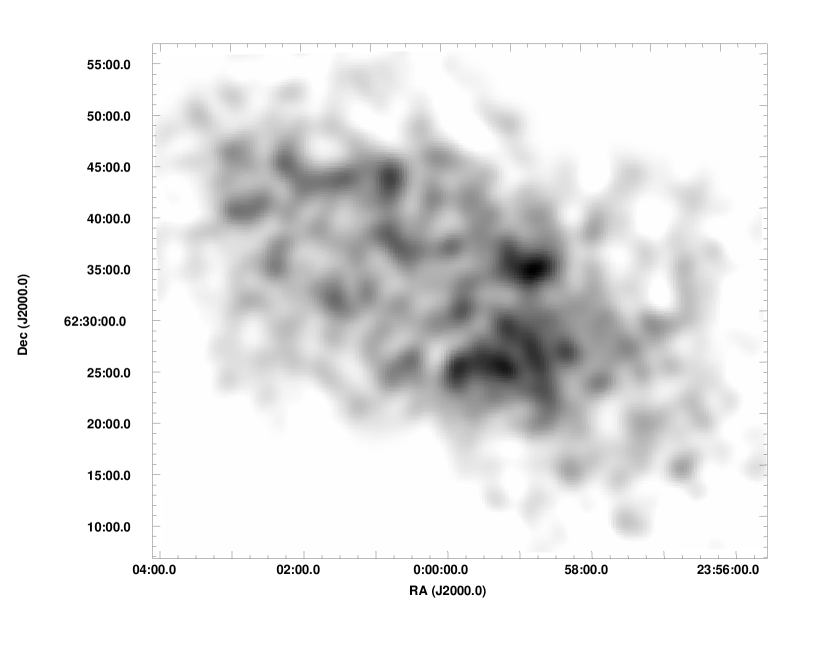
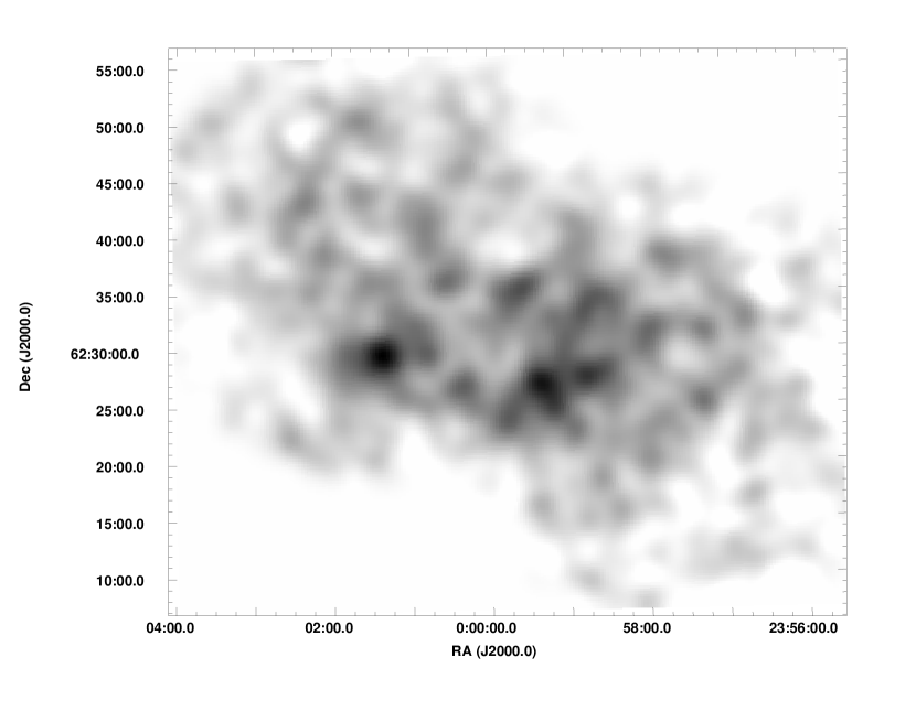
Figure 8: Mosaicked soft band (E$<$1 keV – top) and hard band (E$>$1 keV – bottom) GIS images of CTB 1: both images have been smoothed with a 1$\arcmin$ FWHM Gaussian. The intensity ranges are 0 – 6.42$\times$10^-5 and 0 – 2.85$\times$10^-5 counts sec^-1 arcmin^-2, respectively. The discrete source 1WGA J0001.4$+$6229 (located at RA (J2000.0) 00^h 01^m 25^s.5, Dec (J2000.0) $+$62^∘ 29$\arcmin$ 40$\arcsec$) becomes more prominent at higher energies: this source is discussed in detail in Section 4.

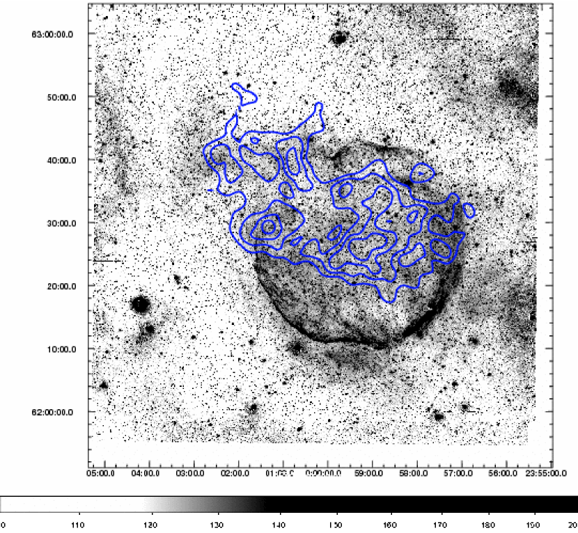
Figure 9: H$\alpha$ image of CTB 1 in greyscale (courtesy of Robert Fesen) with blue ASCA GIS contours overlaid. The contour levels are 2.05, 3.04, 4.02 and 5.01 $\times$ 10^-5 counts sec^-1 arcmin^-2. Notice how the X-ray emission extends through the prominent gap of optical emission.

A broadband (0.7–10.0 keV) exposure-corrected and mosaicked ASCA GIS image of CTB 1 is presented in both Figures 6 and 7 with radio contours from the CGPS overlaid. Both HB21 and CTB 1 show the typical center-filled X-ray morphology combined with a shell-like radio morphology that characterizes MM SNRs: in the case of CTB 1, however, as noted previously the X-ray emission is seen to extend through a gap along the northeastern portion of the radio shell. Figure 8 shows mosaicked images of the soft and hard X-ray emission (again corresponding to the energy ranges E$<$1 keV and E$>$1 keV, respectively); there is a noticeable difference in the spatial structure between the soft and the hard emission. In Figure 9 we present an optical H$\alpha$ image of CTB 1 (courtesy of Robert Fesen) with the contours of the X-ray emission overlaid: the optical morphology of CTB 1 is quite similar to the radio morphology with the same shell-like structure and a prominent gap in the northeast (Fesen et al., 1997). Little H$\alpha$ emission is seen in the interior of CTB 1, nor is any optical emission seen where the X-ray emission extends through the gap in the optical and radio shell in the northeast. The observed slight extension of X-ray emission in the west through the optical and radio shell is likely either residuals due to the broad ASCA point-spread-function or point sources rather than true emission from the SNR. The ASCA hard image reveals a point-like source seen in projection against the diffuse emission of CTB 1: it is located at RA (J2000.0) 00^h 01^m 25.^s5, Dec (J2000.0) $+$62^∘ 29$\arcmin$ 40$\arcsec$ and it lies very close to the eastern edge of the optical and radio shell. This source (denoted as 1WGA J0001.4$+$6229) may be a neutron star possibly associated with CTB 1; we discuss it in detail in the next section. In contrast to HB21, a significant amount of emission from CTB 1 is seen at energies above 1 keV.

Similar to our spectral analysis performed with HB21, we extracted GIS2 and GIS3 spectra from elliptical regions approximately 23$\arcmin$ in size from both the southwestern and northeastern portions of the X-ray emitting plasma. When extracting GIS2 and GIS3 spectra from the northeastern region, we excluded a region 4 arcminutes in diameter centered on the position of the discrete X-ray source 1WGA J00001.4$+$6229 to avoid spectral contamination by this source. We also extracted SIS0 and SIS1 spectra from both the southwestern and northeastern portions of the SNR, again using square-shaped regions approximately 10 arcminutes on a side. Unfortunately, the signal-to-noise ratio of the extracted SIS0 and SIS1 spectra for the northeastern region was not sufficient for spectral analysis and we therefore omitted these spectra from our analysis. We attempted to fit the extracted ASCA spectra using the thermal models VAPEC and VNEI along with the model PHABS for the photoelectric absorption. In contrast to HB21, our fits with either VAPEC or VNEI did not produce a $\chi$${}^{2}_{\nu}$ lower than 1.3 for either region and failed to account for the hard X-ray emission seen above $\sim$3 keV from both regions. A two-component model with a soft thermal component with a temperature of 0.3-0.4 keV (either VAPEC or VNEI) and a second thermal component with a higher temperature or a power law component was required for an acceptable fit to the extracted spectra from both the southwest and northeast portions of the SNR (see Table 4). Thus, a hard excess is present in the ASCA spectra of CTB 1: Lazendic & Slane (2006) also identified a second thermal component of X-ray emission from this SNR based on analysis of extracted ASCA spectra but only for the southwestern region. This hard X-ray emission was not detected previously because the X-ray observatories employed in prior observations of CTB 1 (such as ROSAT) lacked the required sensitivity at high energies.

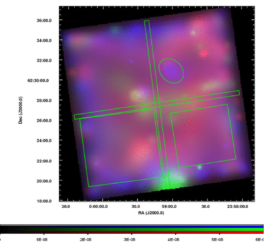
Figure 10: Three-color exposure-corrected and smoothed Chandra image of the interior of CTB 1. This image has been made using monoenergetic exposure maps. Red, green and blue colors correspond to soft (0.5-1.0 keV), medium (1.0-2.0 keV) and hard (2.0-8.0 keV) emission, respectively. The three regions (in green) of spectral extraction are indicated: clockwise from upper left, these are the regions denoted as “hard,” (I1 chip), “soft” (I3 chip) and “diffuse” (I2 chip) excluding point sources (see Section 3.2). The boundaries of the Chandra chips are marked with thin boxes (in green). Note how clumpy features with different spectral properties can be distinguished by noticeable differences in their colors. See Section 3.2.

We examine first the high-spatial resolution Chandra data before discussing the hard emission in more detail. In Figure 10 we present a three-color Chandra image of the interior X-ray emission surrounded by the well-defined optical and radio shell of CTB 1. To illustrate the spectral properties of this emission, in this Figure we have depicted soft (0.5-1.0 keV), medium (1.0-2.0 keV) and hard (2.0-8.0 keV) emission in red, green and blue, respectively. Many features with different spectral properties are visible: most importantly, features with primarily medium and hard spectra are clearly mixed together within the X-ray plasma. At the angular resolution of Chandra, the hard emission (such as the structure $\sim$ 1 arcminute in size located at approximately RA (J2000.0) 23^h 59^m 01.0^s, Dec (J2000.0) $+$62^∘ 30$\arcmin$ 57$\arcsec$) is clearly diffuse and not point-like.

To investigate variations in the spectral properties of the X-ray-emitting plasma of CTB 1 as revealed by Chandra, we extracted spectra from three different Chandra chips. These three extraction regions are as follows: the first region (which we refer to as the “diffuse” region) is on the ACIS-I2 chip and covers most of the area of this chip. A second region (which we refer to as the “soft” region) is located on the ACIS-I3 chip and covers most of the area of that chip as well. Lastly we extracted spectra from a third region (which we will call the “hard” region) which corresponds to a region of hard emission mentioned above and is located on the ACIS-I1 chip: the positions of all three regions are indicated in Figure 10. A region of excess medium energy seen toward the middle of the field in Figure 10 largely fell into gaps between the Chandra detector chips: for this reason, a detailed analysis of its X-ray spectrum could not be conducted.

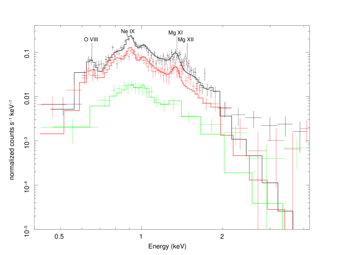
Figure 11: Chandra spectra of the three different regions of CTB 1. The black, red and green lines correspond to spectra from the “diffuse,” “soft” and “hard” regions, respectively. The spectra have been fit with a PHABS$\times$VAPEC model with the temperature of 0.28, 0.28 and 0.66 keV, respectively. The detailed parameters for these fits are given in Table 3.

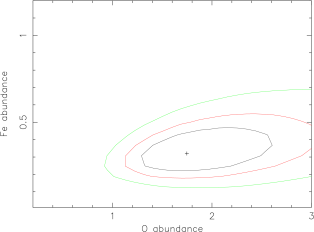
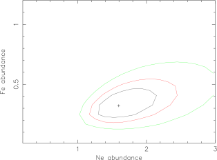
Figure 12: Confidence contours of O and Fe abundances and Ne and Fe abundances, respectively, showing enhanced O and Ne abudances and lower Fe abundance relative to solar, for the PHABS$\times$VAPEC fit to the spectrum extracted for the “diffuse” region. The confidence contours are at the 1$\sigma$, 2$\sigma$ and 3$\sigma$ levels. See Table 3.

We present the extracted spectra of all three regions in Figure 11: spectral variations are present across the X-ray emitting plasma of CTB 1. For example, the spectrum from the “diffuse” region shows prominent O Ly $\alpha$ (0.65 keV), Ne IX (0.9 keV), and Mg XIII (1.35 keV) lines, together with Fe L-shell line emission: in this spectrum the O and Ne lines are stronger than the Fe L-shell line emission. In contrast, the lines are hardly noticeable in the “hard” region spectrum. We derived an acceptable fit to the spectrum of the diffuse region using a thermal model (VAPEC) with a temperature ${\it kT}$ = 0.28$\pm$0.03 keV and $N$_H = 0.64$\pm$0.08$\times$10²² cm^-2; this fit reveals enhanced oxygen and neon abundances and a low iron abundance (see Table 3). The column density $N$_H=0.64$\pm$0.08 $\times$ 10²² cm^-2 is consistent with the optical extinction of E(B-V)=0.7-1 derived by Fesen et al. (1997), which is equivalent to $N$_H$\sim$0.5-0.7 $\times$ 10²² cm^-2. In Figures 12a and 12b, we present confidence contour plots for the abundances of oxygen compared to iron and neon compared to iron (respectively) based on the fit derived from the PHABS$\times$VAPEC model to the spectrum of the “diffuse” region. These figures show that the oxygen and neon abundances are both above solar while the iron abundance is below solar: such relative abundances are a typical characteristic of oxygen-rich SNRs (Woosley & Weaver, 1995).

Our detection and analysis presented here of probable oxygen-rich ejecta in CTB 1 is the first detailed study presented of oxygen-rich ejecta associated with an MM SNR. Based on X-ray spectral analysis, Lazendic & Slane (2006) suggested that another MM SNR – HB 3 – may also feature oxygen-rich ejecta, though those authors could not determine if the plasma associated with that SNR has significantly enhanced abundances of oxygen, neon and magnesium or marginally enhanced abundances of magnesium and underabundant iron. The Chandra spectra are not well fit by a single temperature thermal model (see the poor match to the Mg XII Ly$\alpha$ line as seen in Figure 3), so it is not possible to have oxygen, neon and magnesium all residing in the same constant temperature plasma in ionization equilibrium. Magnesium appears to be more ionized than neon. This may be caused by higher temperatures in magnesium-rich ejecta than in the oxygen- and neon-rich ejecta. It is also possible that the high temperature plasma could be overionized; an overionized plasma has been reported in the MM SNR IC 443 (Kawasaki et al., 2002). When we fit the spectrum of the “soft” region using a VAPEC model combined with the PHABS model for the interstellar photoelectric absorption, the iron abundance is higher and the neon abundance is lower when compared with the “diffuse” region spectra (see Table 3), suggesting spatial variations in the chemical composition within the X-ray emitting gas of CTB 1.

Lastly, we describe the spectral analysis of the third (“hard”) region which features a harder spectrum when compared to the other two spectra (see Figure 11). Such localized hard emission has been reported in several other MM SNRs, either as non-thermal diffuse knots seen in XMM-Newton observations of IC 443 (Bocchino & Bykov, 2003) or as a pulsar wind nebula (also in IC 443 – Olbert et al. (2001)). Because of the lack of lines in the spectrum, we first fit the spectra with a power law, which resulted in an acceptable fit, but with an unrealistically high photon index of $\Gamma$$\sim$6.4${}^{+5.6}_{-2.9}$ (see Table 3). In comparison, a VAPEC thermal model yielded a comparable-quality fit with a temperature of $\it{kT}$ = 0.66${}^{+0.27}_{-0.41}$ keV: for this fit, we froze the abundance of oxygen to 1.7 (to be consistent with the fits derived to the spectra of the “diffuse” and “soft” regions) or 1 while fitting for the abundances of neon and iron. We also fit the spectrum of this region with a combination of an APEC thermal component and a non-thermal power-law component; to reduce the number of free parameters we fixed the temperature of the thermal component to ${\it kT}$ = 0.28 keV, equal to the temperature derived from fits to the other two regions. The results are given in Table 3: unfortunately, we do not have enough counts in the spectrum of the “hard” region to distinguish between non-thermal and thermal interpretations of the spectrum of this source. However, the temperature derived from the thermal fit ($kT$ = 0.66 keV) is significantly higher than the temperature of the “soft” and “diffuse” regions. Also, thermal models systematically underpredict Chandra spectra at high energies in all the regions: we interpret this result as evidence that the hard excess observed toward CTB 1 has a diffuse origin.

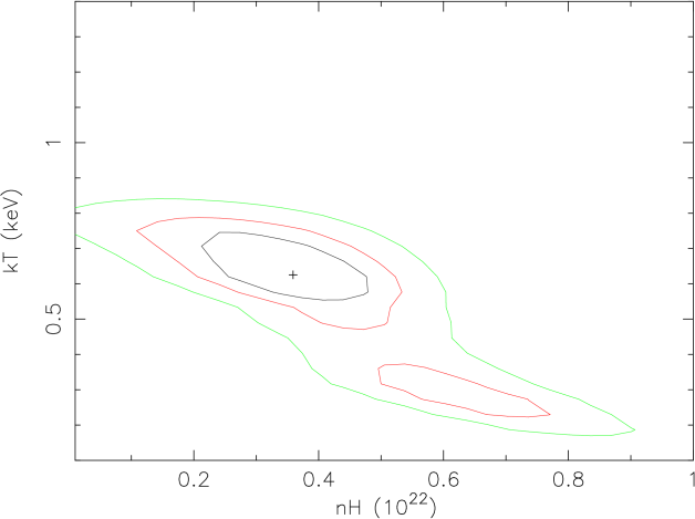
Figure 13: Confidence contours for the line-of-sight column density $N$_H and the temperature $kT$ for the PHABS$\times$VAPEC spectral fit (with fixed solar abundances) to the spectrum of the “hard” region (see Table 3). Notice the bimodality for components with temperatures of $kT$ $\sim$ 0.28 keV and $kT$ $\sim$ 0.66 keV: this may indicate a presence of an additional thermal component besides the thermal component identified in the fit of the spectrum of the “diffuse” region. The confidence contours are at the 1$\sigma$, 2$\sigma$ and 3$\sigma$ levels. See Section 3.2.

In Figure 13, we present a plot of confidence contours for $N$_H and $kT$ that correspond to the fit to the spectrum of the “hard” region as fit with the PHABS$\times$VAPEC model with fixed solar abundances. The spectrum of this region demonstrates a bimodality with temperatures of $kT$ $\sim$ 0.28 and $kT$ $\sim$ 0.66 keV, suggesting the presence of an additional component in addition to the thermal component associated with the “diffuse” region. We will discuss the nature of this hard component further below and in Section 7. We also note differences between our results from analyzing Chandra ACIS-I spectra and the results presented by Lazendic & Slane (2006): those authors jointly fit four spectra taken from each ACIS-I chip (they did not attempt any spectral analysis of small regions like the “hard” region”) and presented an acceptable fit obtained using two VNEI components: one with a temperature $kT$ = 0.20${}^{+0.04}_{-0.01}$ keV and solar abundances and the other with a temperature $kT$=0.86${}^{+0.03}_{-0.06}$ and an elevated magnesium abundance (Mg=3.1${}^{+1.0}_{-0.4}$). Those authors did comment on the presence of lines associated with oxygen as well as the neon and iron line blend in the extracted ACIS spectra but they did not present an analysis of the abundance of those elements.

After establishing the spectral properties of the soft X-ray emitting plasma from Chandra spectra, we fit the ASCA GIS2/3 and SIS0/1 spectra of the southwestern portion of CTB 1. We froze the oxygen abundance to 1.7 (or 1) for all spectral fits while allowing the neon and iron abundances to vary. Because models with a single thermal component were not sufficient to describe the X-ray spectra, we used a combination of the thermal models VAPEC and VNEI along with a power law model to jointly fit the ASCA spectra: the results of these spectral analyses are given in Table 4. From these fits, we estimate a column density $N$_H $\sim$ 0.5-0.6 $\times$ 10²² cm^-2 and a temperature $\it{kT_{\rm{soft}}}$ $\sim$ 0.2-0.3 keV for the soft emission. The soft thermal component has most likely attained thermal equilibrium because fits to this soft emission using the VNEI model resulted in a long ionization timescale ($\tau$ $\sim$ 1 ($>$0.2) $\times$ 10¹¹ cm^-3 s). The hydrogen column density $N$_H and the temperature of the soft component $\it{kT_{\rm{soft}}}$ are in agreement with the analysis of ROSAT spectra (Rho, 1995; Craig et al., 1997). The inclusion of a second component was necessary for obtaining statistically-acceptable fits to the ASCA spectra of the southwestern region (with values for the $\chi$${}^{2}_{\nu}$ $\sim$1.1): the addition of a power law with a photon index $\Gamma$ $\sim$ 2-3 or a second thermal component with a temperature ${\it kT}$ $\sim$ 3 keV yields fits with a comparable quality. Unfortunately due to a low number of counts in the spectra at the higher X-ray energies, we cannot distinguish between different models for the high-energy emission. In Figure 14 we present the GIS and SIS X-ray spectra of the southwest region, fit with the combination of a thermal (VAPEC) and non-thermal (power law) model. Our results differ from Lazendic & Slane (2006) who fit the extracted ASCA spectra from this region with two thermal components in CIE: the softer temperature component featured a temperature $kT$ = 0.19${}^{+0.09}_{-0.03}$ keV and a magnesium abundance fixed at solar while the harder temperature component featured a temperature $kT$=0.82${}^{+0.09}_{-0.06}$ keV and an elevated magnesium abundance (Mg=2.7${}^{+0.9}_{-0.5}$).

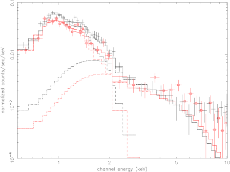
Figure 15: ASCA GIS2 spectra of the southwest (in black with crosses) and northeast (in red with squares) regions of CTB 1. Both of these spectra have been fit with a PHABS$\times$(VAPEC+POWER LAW) model. The parameters of the fits to these spectra are listed in Table 4.

Finally, we examine the ASCA spectra of the northeast region of CTB 1 which corresponds to the known “break-out” site seen in optical and radio images of this SNR.. Like the southwest region, a second component is needed (in addition to a soft thermal component) to derive a statistically acceptable fit. A fit to these spectra using a power-law component for the hard emission is presented in Table 4 and the GIS spectra are presented in Figure 15. For the thermal component we have first assumed the abundances of oxygen, neon and iron to be 1.7, 1.6 and 0.4, respectively, equal to the abundances in the “diffuse” region. Secondly, we assumed solar abundances for the hard component. Although the GIS spectra of the northeastern region feature a stronger Fe L-shell line complex when compared with the spectra of the southwestern region, our spectral fits could not confirm non-solar abundances and the abundances are consistent with solar values.

The photon index derived from fits to the northeast is flatter than the photon index derived from fits for the southwest region: $\Gamma=1.4$ compared to $\Gamma=2-3$, respectively. However, the photon statistics at higher energies is poor, making it difficult to determine the true nature of this hard emission. Although the northeast region does correspond to the prominent breakout feature, we do not find evidence for any major differences in the X-ray properties between the northeast and southwestern regions of CTB 1. The fact that no significant variations are seen on large scales in the X-ray properties of CTB 1, coupled with the variations seen on small scales as revealed by the Chandra observation, indicate that the X-ray emission from this SNR is complex. A parallel may be drawn with the results from Chandra observations of 3C 391, another MM SNR: in the case of that source, local spectral differences appeared to be stronger than global ones (Chen et al., 2004). Here again we find that our results differ from those presented by Lazendic & Slane (2006): for this region, the authors derived an acceptable fit using a single thermal component ($kT$ = 0.18${}^{+0.00}_{-0.01}$ keV) in CIE with solar abundances.

4 1WGA J0001.4+6229 – An X-ray Pulsar Associated with CTB 1?

The ASCA hard energy image ($E$ $>$ 1 keV) revealed a hard source in the northeastern region of CTB 1 which is located just inside the eastern shell of the SNR: the position of this source is RA (J2000.0) 00^h 01^m 25.^s5, Dec (J2000.0) $+$62^∘ 29$\arcmin$ 40$\arcsec$ with a positional uncertainty of 13$\arcsec$. This is the discrete X-ray source 1 WGA J0001.4$+$6229 in the Catalog of ROSAT PSPC WGA Sources (White et al., 1994, 1997; Angelini et al., 2000). This X-ray source may possibly be a neutron star associated with CTB 1. We therefore conducted spectral and timing analysis of the X-ray emission from this source using the ASCA GIS2 and GIS3 datasets.

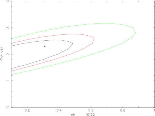
Figure 16: (left) The GIS2/GIS3 spectra of the hard source 1WGA J0001.4$+$6229 as fit with an absorbed power-law model. (right) Plot of confidence contours for Photon Index versus $N_{H}$ for this fit: a low column density is implied, indicating that the source is Galactic rather than extragalactic. The confidence contours are at the 1$\sigma$, 2$\sigma$ and 3$\sigma$ levels. See Section 4.

The procedure for extracting GIS2 and GIS3 spectra of 1WGA J0001.4$+$6229 and performing a spectral analysis was the same as for extracting GIS2 and GIS3 spectra of the diffuse emission from HB21 and CTB 1: a circular region four arcminutes in diameter centered on the source position was used to extract spectra. The total number of counts and the corresponding count rate (over the energy range from 0.6 keV to 10 keV) for our GIS2 and GIS3 observations were 115 and 103 counts, and 5.71$\pm$0.53$\times$10^-3 and 5.11$\pm$0.51$\times$10^-3 counts per second, respectively. We derived a statistically-acceptable joint fit to the spectra using a simple power law model combined with the same PHABS model mentioned previously for the photoelectric absorption along the line of sight. The parameters of this fit were a column density of $N$_H=0.3 ($<$0.65$)\times 10^{22}$ cm^-2 and a photon index $\Gamma$=2.2${}^{+0.5}_{-1.2}$: in Figure 16 we present the extracted GIS2/GIS3 spectra together with the best-fit model, and a confidence contour plot for $N$_H and $\Gamma$. The derived photon index is typical for rotation-powered pulsars. The column density is consistent with the range of column densities derived in our fits (see Tables 3 and 4) to the CTB 1 spectra, hinting at a possible association. If we fit the extracted spectra for this source with a blackbody model, a temperature of kT$\sim$1.1 keV is derived (although this fit with $\chi$${}^{2}_{\nu}$=0.92 for 48 degrees of freedom (DOF) is inferior to the power-law fit with $\chi$${}^{2}_{\nu}$=0.79). Because of the low derived column density, our estimated absorbed and unabsorbed fluxes for this source are virtually identical: for the GIS2 (GIS3) spectrum, the flux is 5.4$\times$10^-13 (6.4$\times$10^-13) ergs cm^-2 sec^-1; at the assumed distance to CTB 1, these fluxes correspond to luminosities of 6.2$\times$10³² (7.4$\times$10³²) ergs s^-1, respectively. We also performed a timing analysis using the GIS2/GIS3 datasets to search for pulsed X-ray emission from this source and detected a period of 47.6154 milliseconds using the Rayleigh test (a maximum signal of $Z$² = 31.4), but the detection is not statistically significant.

We further searched for pulsations from 1WGA J0001.4$+$6229 with the 100-meter Green Bank Telescope (GBT) of the National Radio Astronomy Observatory (NRAO) on 2004 December 7. The target position was observed for 7.6 hours at a center frequency of 825 MHz. The frontend was the GBT Prime Focus 1 receiver to feed the Pulsar Spigot (Kaplan et al., 2005) and Berkeley-Caltech Pulsar Machine (BCPM) backends. The receiver provided 50 MHz of bandwidth in two orthogonal polarizations that were summed and synthesized into 1024 frequency channels every 81.92 $\mu$s in the Spigot and 96 channels of 0.25 MHz width every 144 $\mu$s in the BCPM. The interstellar dispersion toward CTB1 is unknown, but we can estimate it with the latest model of Galactic electron density (Cordes & Lazio, 2002), which predicts a dispersion measure (DM) of 105 pc cm^-3 for a distance of 3.1 kpc or DM = 33 pc cm^-3 at a distance of 1.6 kpc (corresponding to the two distances to CTB 1 that have been published in the literature). We therefore take a conservative upper limit of DM = 1000 to CTB 1 (given the narrow channels and relative long pulsation period the search is not highly DM dependent). The data set was dedispersed with DMs from 0 to 1000 and searched for periodicities using standard folding and fast Fourier-Transform (FFT)-based techniques. Based on these analyses, we find no significant evidence for pulsations with any period from 1WGA J0001.4$+$6229.

Assuming that 1WGA J0001.4$+$6229 is in fact a neutron star associated with CTB 1, a transverse velocity can be estimated. The angular displacement of 1WGA J0001.4$+$6229 from the center of CTB 1 is 14^′ while the radius of the SNR itself is 17^′. Therefore, we calculate a transverse velocity $v$ = 850 d_3.1 t${}_{1.6}^{-1}$ km s^-1, where d_3.1 is the distance to CTB 1 in units of 3.1 kpc and t_1.6 is the age of the SNR (Fesen et al., 1997) in units of 1.6 $\times$ 10⁴ yr. This estimated transverse velocity is high but this may be an overestimate because of the considerable uncertainties associated with estimates of the distance and age of CTB 1: if we assume a distance to the SNR of 1.6 kpc, the tranverse velocity is only 420 km s^-1. In particular, the published age estimates are based on simple one-dimensional SNR models: the obvious breakout morphology of CTB 1 clearly indicates that such models are not applicable in this case. For comparison, the transverse velocities for neutron stars located off center in their associated SNRs are 375 km s^-1 in the case of the SNR W44 (Frail et al., 1996) and 250$\pm$50 km s^-1 in the case of the SNR IC 443 (Olbert et al., 2001). It is plausible that 1WGA J0001.4$+$6229 is associated with CTB 1 but deeper high-spatial resolution X-ray observations are needed to examine its spectrum in more detail and search for possible pulsations.

5 Plasma Conditions in HB21

We first estimate the density and mass of the X-ray emitting plasma associated with HB21 based on the emission measures derived from our spectral fitting. Our GIS spectral extraction regions extend over approximately 11$\farcm$5 $\times$ 11$\farcm$5 or 5.7 pc $\times$ 5.7 pc (2.7 pc $\times$ 2.7 pc) at the assumed 1.7 (0.8) kpc distance to HB21. Assuming a cylindrical geometry with the long axis equal to the observed extent of the X-ray plasma (35$\farcm$8, corresponding to 17.7 (8.3) pc), the volume of each region is approximately 5.4$\times$10⁵⁸ (5.6$\times$10⁵⁷) cm³. From the mean values of our derived emission measures (which are approximately the same for all regions and all models), we calculate an electron density $n$_e $\approx$ 0.06 (0.08) cm^-3 (where we have assumed $n$_e $\approx$ 1.2$n$_H) and a volume filling fraction of unity based on the smooth appearance and isothermal nature of the X-ray emitting gas. Based on this value, we estimate the total mass of the X-ray emitting plasma within the field of view of the ASCA observations to be only $\approx$$2.6(1.5)M_{\odot}$. When we account for the incomplete spatial coverage of HB21 by the ASCA observations, the total X-ray mass could be higher by a factor of 9, which amounts to a total of 23.4 (14) $M_{\odot}$. The corresponding Si and S masses are $1.7\times 10^{-3}M_{\odot}$ and $1.3\times 10^{-3}M_{\odot}$, respectively. The presence of a bright radio shell without associated X-ray emission combined with the detections of an expanding HI shell and infrared emission from shock-cloud interaction regions (Koo & Heiles, 1991; Shinn et al., 2009, 2010, and the references therein) imply that HB21 is in a radiative cooling stage. The SNR age inferred from the presence of an expanding ($v_{exp}=124$ km s^-1) HI shell is $t$_d = 4.5$\times$10⁴ yr (Koo & Heiles, 1991). We can also infer the pressure within HB21 from properties of the X-ray emitting gas. The total number of particles is $n$_total = $n$_e+$n$_H+$n$_He$\approx$2$n$_e for a plasma with cosmic abundances: from our estimated values for electron density and temperature, the corresponding pressure is P/k = 2$n$_e$T$ = 0.9 (1.2)$\times$10⁶ K cm^-3, which as about two orders of magnitude higher than the typical ISM pressure. The physical properties of HB21 are summarized in Table 5.

The X-ray properties of HB21 are similar to those measured for many other MM SNRs. First, the presence of an isothermal plasma with a temperature of $kT$ $\sim$ 0.2-0.7 keV is consistent with other MM SNRs such as 3C391 (Rho & Petre, 1996; Chen et al., 2004), W44 (Rho et al., 1994; Shelton et al., 2004), 3C400.2 (Yoshita et al., 2001), W51C (Koo et al., 2002), W63 (Mavromatakis et al., 2004), and Kes 79 (Sun et al., 2004). This result supports the interpretation that these SNRs are evolved and in the radiative phase as suggested by the presence of infrared, optical and HI shells for many of these SNRs. There are no temperature variations and no pronounced enhancements of chemical abundances in HB21 either, just as in many other MM SNRs like 3C 391. These properties of HB21 exemplify the typical X-ray properties characteristic of MM SNRs as defined by Rho & Petre (1998). At a sufficiently old age ($\sim 10^{6}$ yr) age, a SNR should exhibit a centrally-filled X-ray morphology and eventually merge with the hot ISM gas (Cui & Cox, 1992): however, MM SNRs attain this state at a much earlier age ($\sim 10^{4}$ yr). When a distance of 1.7 kpc to HB21 is assumed, the calculated X-ray emitting mass of this SNR is comparable to those of other MM SNRs. For standard radiative SNR models, we expect $\sim 100$ M_⊙ of X-ray emitting gas at the HB21 age of $4\times 10^{4}$ yr based on equations given by Cui & Cox (1992) and models presented by Hellsten & Sommer-Larsen (1995). Even more X-ray emitting gas is expected in conduction models of Cox et al. (1999). This discrepancy between the observed and predicted X-ray emitting mass is also present in W28 (Rho & Borkowski, 2002), but unlike in W28 (where large temperature gradients have been detected), the presence of an isothermal plasma at the center of HB21 suggests that the electron thermal conduction is important (Chevalier, 1999). The conduction model of Cox et al. (1999) overpredicts the mass of X-ray emitting gas: however, this model assumes a uniform ambient ISM while HB21 is known to be interacting with with clumpy molecular clouds (Koo et al., 2001; Shinn et al., 2009, 2010). More elaborate X-ray emission models of SNRs in molecular clouds are needed to account for the observed X-ray properties of HB21 and similar MM SNRs.

6 Supernova Ejecta in CTB 1

The enhanced abundances of oxygen and neon and low iron abundances in the “diffuse” region (see Table 3) indicate that CTB 1 is likely an oxygen-rich SNR. This SNR was likely produced by a core-collapse SN explosion, because such explosions produce O- and Ne-rich, and Fe-poor ejecta (Nomoto et al., 1997; Woosley & Weaver, 1995). This finding is consistent with the presence of a massive star forming environment near CTB 1 (Landecker et al., 1982): in addition, the scenario for the creation of this SNR by a core-collapse SN explosion would be further supported if the discrete X-ray source discussed earlier – 1WGA J0001.4$+$6229 – is shown to be a neutron star associated with this SNR. Examples of oxygen-rich SNRs include young sources like Cas A, N132D, and E0102.2$-$72.3; recently two older SNRs located in the Small Magellanic Cloud (SMC) – SNR B0049-73.6 (Hendrick, Reynolds, & Borkowski, 2005) and B0103-72.6 (Park et al., 2003) – were also classified as oxygen-rich SNRs. Both of these SMC SNRs show the ejecta material in their interiors surrounded by shells of swept-up ambient material at relatively low X-ray emitting temperatures. An X-ray emitting shell might be present in CTB 1, but its detection may be prevented by substantial interstellar absorption in this direction combined with an expected low temperature of the shocked ambient gas.

We estimated the X-ray mass and density of CTB 1 from our fits to the ASCA spectra, assuming metal abundances derived from the Chandra spectra of the “diffuse” and “soft” regions. The spectral fits to the GIS spectra in the 11$\farcm$5 $\times$ 11$\farcm$5 region imply an electron density of $0.16f^{-1/2}_{soft}$ cm^-3 for the soft thermal component (where $f_{soft}$ is the volume filling factor for this component). The corresponding hydrogen density $n_{H}$ is equal to $n_{e}/1.2=0.13f^{-1/2}_{soft}{\rm cm}^{-3}$; based on this value we estimate the total mass of the X-ray emitting plasma to be $\approx 40f^{1/2}_{soft}M_{\odot}$. From our derived abundances of oxygen, neon and iron based on Chandra data, we estimate the oxygen, neon and iron masses to be $0.66f^{1/2}_{soft}$, $0.11f^{1/2}_{soft}$, and $0.03f^{1/2}_{soft}$ M_⊙, respectively. The ratio of [O/Fe] is 4.3${}^{+10.2}_{-2.5}$ and [Ne/Fe] is 4.0${}^{+8.0}_{-2.2}$ for CTB 1. The expected ratio of [O/Fe] is 0.75 for a Type Ia explosion and greater than 4 for a core-collapse explosion. These abundances imply that CTB 1 is a remnant of a core-collapse explosion and are consistent with the predictions for a stellar progenitor with a mass of 13 - 15 M_⊙ (Woosley & Weaver, 1995; Nomoto et al., 1997), but higher mass stellar progenitors are not excluded.

Finally, we estimate the pressures of the soft and hard components of the X-ray emitting gas using the parameters of the PHABS$\times$(VAPEC+VAPEC) model: for the soft component we calculate a corresponding pressure P/k = 1.1$\times$10⁶ $f$${}_{soft}^{-1/2}$ K cm^-3. For the hard component (assuming a thermal origin), we first need to calculate the corresponding electron density which we can determine from the electron density of the soft component and the emission measures (EMs) of the soft and hard components (i.e., $n_{e}$(hard) = $n_{e}$(soft) [EM_hard/EM_soft]^1/2). From this relation, we obtain $n$_e(hard) = 0.029 $f$${}_{hard}^{-1/2}$ cm^-3 (here $f$_hard is the volume filling factor for the hard component) and therefore a corresponding pressure P/k = 2.0$\times$10⁶ $f$${}_{hard}^{-1/2}$ K cm^-3. This result implies a factor of four larger filling factor for the hotter gas than the cooler gas if these two components are in pressure equilibrium: a higher filling factor for the hot gas is typical. Assuming $f_{soft}+f_{hard}=1$, pressure within CTB 1 is $2.8\times 10^{6}$ K cm^-3. We summarize these inferred physical properties for CTB 1 in Table 5.

CTB 1 therefore belongs to a growing number of known evolved SNRs which feature an enhanced metal abundance in their interiors. An example of another MM SNR which features such enhanced abundances is W44 (Shelton et al., 2004): other similar sources are identified by Lazendic & Slane (2006) (including HB21, which was analyzed both in their study and in the study presented here.) In addition, two other Galactic SNRs – the Cygnus Loop (Miyata et al., 1998) and G347.7$+$0.2 (Lazendic et al., 2005) – feature enhanced abundances of metals as well. W49B (Hwang et al., 2000) shows highly enhanced abundances but its age is estimated to be 2000 years (Hwang et al., 2000) and Rho & Petre (1998) describe the source as an atypical MM SNR. Because MM SNRs like CTB 1 are commonly believed to be evolved sources – age estimates of CTB 1 range from 9000 yr (Craig et al., 1997) to 4.4$\times$10⁴ yr (Koo & Heiles, 1991) – their X-ray spectra are dominated by swept-up material (Rho & Petre, 1998). Therefore, the detection of X-ray-emitting material associated with these sources with enhanced metal abundances is unexpected. The detection of O-rich ejecta associated with CTB 1 is particularly noteworthy: CTB 1 may belong to a previously unrecognized class of MM SNRs whose X-ray emission is dominated by O-rich ejecta located within their interiors. As noted previously, another possible member of this particular class of MM SNRs with O-rich ejecta may be HB3 (Lazendic & Slane, 2006). We note that O-rich ejecta has been previously detected in the evolved (1.4 $\times$10⁴ yr old) SMC SNR B0049-73.6 by Hendrick, Reynolds, & Borkowski (2005) and it is likely that centrally-located ejecta will be found in a number of relatively old Galactic SNRs.

The X-ray emitting plasma associated with CTB 1 clearly extends through the gap in the crescent-shaped radio shell: Hailey & Craig (1994) and Rho (1995) first noticed this remarkable extension of X-ray emission based on ROSAT PSPC observations. Two scenarios have been proposed to explain the morphology of the observed X-ray emission: Craig et al. (1997) has suggested that the ambient ISM toward the northeastern portion of the SNR was cleared by a supernova event which took place prior to the birth of CTB 1, and thus a breakout occurred as the SNR expanded into this region of a dramatically lower density. A competing theory for the morphology has been proposed by Yar-Uyaniker et al. (2004), who suggested that the X-ray emission from CTB 1 lies in the interior of a bubble seen in the 21 cm H line, presumably blown by winds of the CTB 1 stellar progenitor. Our X-ray images show that the diffuse X-ray emission in the northeast clearly extends through the relatively narrow break in the optical and radio shell, with the breakout directed into the interior of the bubble seen in the neutral hydrogen line. Such a morphology favors a scenario where a supernova explosion occurred within the HI shell, followed by subsequent breakout into the bubble and not an explosion within the bubble itself. Our ASCA spectra show little difference between the X-ray properties of the southwest and northeast regions: hints of variations in temperature and abundances exist but better X-ray data are needed to determine whether they are real and not just statistical fluctuations.

7 The Nature of the Hard X-ray Emission from CTB 1

The ASCA spectra of the southwestern portion of CTB 1 revealed the presence of a hard component in addition to the soft ($kT$ $\sim$ 0.28 keV) component. This hard component may be modeled as a second thermal component with a temperature of $\it{kT}$ $\sim$ 3 keV or as a power-law continuum with a photon index $\Gamma$ $\sim$ 2-3. Hard X-ray emission was also detected by ASCA in the northeast region of CTB 1: a power-law component with a photon index $\Gamma$ $\sim$ 1.4 (a somewhat lower value compared to the southwest region) combined with a soft thermal component (again with a temperature $\it{kT}$ $\sim$ 0.28 keV) yields a statisically acceptable fit. The Chandra observation of the southwest region of CTB 1 revealed regions of harder emission patches on the scale of an arcminute in size: the spectrum of one of these regions can be modeled by either a single thermal component with an elevated temperature ($\it{kT}$ $\sim$ 0.66 keV) or as the combination of a soft thermal component ($\it{kT}$ $\sim$ 0.28 keV) and a power law component with a photon index $\Gamma$ $\sim$ 2.0 (see Tables 3 and 4). The “hard” region observed by Chandra is only a few arcminutes from the center of CTB 1 and well inside the radio-emitting shell of the SNR: it is diffuse in nature although the number of counts detected from the source is limited. It is possible that the hard X-ray emission detected by ASCA from CTB 1 may be composed of localized hard regions such as this one: unfortunately we do not have enough counts in this “hard” region to distinguish between thermal and non-thermal origins. We note that two other MM SNRs, W28 and IC 443, contain high-temperature thermal plasmas in their interiors (Rho & Borkowski, 2002; Kawasaki et al., 2002).

Several possible explanations may be considered for the origin of hard X-ray emission from MM SNRs: first, the hard emission may be caused by temperature variations within the SNR. In the case of CTB 1, this scenario is supported by a good fit to the spectrum of the “hard” region with a thermal component with a much higher than average temperature. Supernova ejecta may be inhomogeneous, in which case a multi-temperature plasma with spatially-varying abundances is expected. Alternatively, the “hard” regions may be caused by localized nonthermal emission: such emission has already been detected in IC 443 (Bocchino & Bykov, 2003) and $\gamma$ Cygni (Uchiyama et al., 2002). Additional observations are needed to understand the true nature of the hard X-ray emission from CTB 1.

8 Summary

1. We presented ASCA observations of the MM SNR HB21. Our ASCA images of this SNR are similar to ROSAT images and reveal a diffuse centrally filled X-ray emission located within a radio shell. From X-ray spectra, we measure a column density toward this source and a temperature for the X-ray emitting plasma of $N$_H $\sim$ 0.3$\times$10²² cm^-2 and $\it{kT}$ $\sim$ 0.7 keV, respectively: no significant spatial differences in temperature are found. Silicon and sulfur abundances are slightly enhanced relative to solar, particularly for the northwestern region, and no hard component to the X-ray emission was detected. The properties of HB21 are similar to those seen in several other MM SNRs, such as the presence of isothermal plasma. This result supports the interpretation that MM SNRs are evolved sources currently in the radiative phase of evolution: the X-ray properties of HB21 exemplify the primary characteristics of MM SNRs as defined by Rho & Petre (1998).

2. We presented ASCA and Chandra observations of the MM SNR CTB 1. ASCA observations reveal center-filled X-ray emission located within the radio shell: the X-ray emission extends outside the circular shell through the breakout gap in the northeast. While the global X-ray and radio morphology is similar to HB21, the X-ray spectra of CTB 1 and HB21 are very different. The X-ray spectrum of CTB 1 shows several prominent lines such as O Ly$\alpha$ (0.65 keV) and Ne IX (0.9 keV). We find that CTB 1 is likely an oxygen-rich SNR with enhanced abundances of oxygen and neon: this is surprising for an evolved SNR such as CTB 1. The derived abundances are consistent with an explosion of a stellar progenitor with a mass of 13 - 15 M_⊙ and possibly even higher.

3. The ASCA spectra of the southwest region of CTB 1 cannot be fit with a single thermal component and instead require the presence of an additional component to account for an excess emission seen at higher energies. Based on ASCA and Chandra spectra of CTB 1, we derive a column density $N$_H $\sim$ 0.6$\times$ 10²² cm^-2 and the soft component temperature $\it{kT}$_soft$\sim$ 0.28 keV; the hard emission may be modeled either by a thermal component with a temperature $\it{kT}$_hard $\sim$ 3 keV or by a power law component with a photon index of $\Gamma$ $\sim$ 2-3. Likewise, the ASCA spectra of the northeast region of CTB 1 also show an excess at higher energies: these spectra are fit best by a power law with a photon index $\Gamma$ = 1.4 plus the soft thermal component. The Chandra observation of the southwestern region reveals localized regions of hard emission: one such region is $\sim 1^{\prime}$ in size. The X-ray spectrum of this region may be fit with either a higher temperature thermal component ($\it{kT}$ = 0.66 keV) or with the combination of a softer thermal component ($\it{kT}$ = 0.28 keV) and a power law component ($\Gamma$ $\sim$ 2.0). Because of the poor photon statistics, its true nature is unclear. Possible scenarios for its origin include temperature variations within the X-ray emitting plasma of CTB 1, including the ejecta, or localized non-thermal X-ray emission.

4. The ASCA hard ($E>1$ keV) image of CTB 1 reveals a point-like source seen in projection against the diffuse emission of CTB 1. This source – denoted as 1WGA J0001.4$+$6229 and located at RA (J2000.0) 00^h 01^m 25.^s5, Dec (J2000.0) $+$62^∘ 29$\arcmin$ 40$\arcsec$ – may be a neutron star associated with CTB 1. The GIS2/GIS3 spectra of this source are well-fit by a power-law continuum with a photon index $\Gamma$=2.2${}^{+0.5}_{-1.2}$ (typical for rotation-powered pulsars) and the measured column density is comparable to the column density measured for CTB 1. There is marginal evidence for pulsations in X-ray data at 47.6 msec, but no pulsations have been detected at radio wavelengths.

Table 1: Summary of ASCA GIS and SIS Observations of HB21 and CTB 1

						GIS2	GIS2	GIS3	GIS3	SIS0	SIS0	SIS1	SIS1
						Effective	Count	Effective	Count	Effective	Count	Effective	Count
				Right		Exposure	Rate	Exposure	Rate	Exposure	Rate	Exposure	Rate
Sequence			Observation	Ascension	Declination	Time	(10-2 cts	Time	(10-2 cts	Time	(10-2 cts	Time	(10-2 cts
Number	SNR	Pointing	Date	(J2000.0)	(J2000.0)	(s)	sec-1)	(sec)	s-1)	(s)	s-1)	(s)	s-1)
55053000	HB21	NW	1997 June 9-10	20 44 53.8	$+$50 54 31	39254	7.38$\pm$0.19	39248	7.31$\pm$0.19	35307	6.78$\pm$0.18	35158	5.55$\pm$0.17
55054000	HB21	SE	1997 June 10-11	20 46 31.4	$+$50 38 43	38415	7.18$\pm$0.19	38413	7.39$\pm$0.19	34448	5.52$\pm$0.17	33940	4.21$\pm$0.16
54026000	CTB1	SW	1996 January 21	23 57 31.9	$+$62 25 20	58065	6.03$\pm$0.15	58078	5.44$\pm$0.14	53592	10.52$\pm$0.15	53746	8.64$\pm$0.13
54027000	CTB1	NE	1996 January 22	00 01 21.9	$+$62 38 52	41637	4.83$\pm$0.16	41649	5.16$\pm$0.17	$\cdots$	$\cdots$	$\cdots$	$\cdots$

Note. — The units of Right Ascension are hours, minutes and seconds and the units of Declination are degrees, arcminutes and arcseconds. Count rates are for the energy range 0.6–10.0 keV.

Table 2: Summary of Fits to GIS and SIS Spectra of HB21

Parameter	GIS2/3+SIS0/1	GIS2/3+SIS0/1	GIS2/3+SIS0/1	GIS2/3+SIS0/1	GIS2	GIS2
Region	Northwest	Northwest	Southeast	Southeast	Northwest	Northwest
					and Southeast	and Southeast
Model	PHABS$\times$	PHABS$\times$	PHABS$\times$	PHABS$\times$	PHABS$\times$	PHABS$\times$
	VAPEC	VNEI	VAPEC	VNEI	VAPEC	VNEI
$\chi$${}^{2}_{\nu}$ ($\chi$2/DOF)	1.05 (1103/1054)	1.05 (1102/1053)	1.06 (1119/1054)	1.04 (1099/1053)	1.06 (340.43/321)	1.05 (336.50/327)
$N$H ($\times$ 1022 cm-2)	0.23$\pm$0.04	0.24${}^{+0.06}_{-0.04}$	0.31$\pm$0.04	0.30$\pm$0.06	0.22${}^{+0.05}_{-0.06}$	0.24$\pm$0.06
${kT}$ (keV)	0.65$\pm$0.03	0.63${}^{+0.03}_{-0.04}$	0.68${}^{+0.03}_{-0.02}$	0.67$\pm$0.04	0.63$\pm$0.06	0.62${}^{+0.06}_{-0.05}$
Si	1.3${}^{+0.3}_{-0.2}$	1.8$\pm$0.5	1.4$\pm$0.3	2.0$\pm$0.4	1.6${}^{+0.5}_{-0.3}$	1.9${}^{+0.5}_{-0.4}$
S	2.4$\pm$1.0	3.6${}^{+1.7}_{-1.9}$	1.7${}^{+0.9}_{-0.8}$	3.0$\pm$1.4	3.4${}^{+1.6}_{-1.4}$	4.3${}^{+1.9}_{-1.8}$
$\tau$ (1011 cm-3 s)	$\cdots$	5.9($>$3.2)	$\cdots$	4.1${}^{+5.9}_{-1.1}$	$\cdots$	350($>$4.0)
EM /(4$\pi$d2/10-14) (cm-5)	4.4$\times$10-3	4.4$\times$10-3	4.7$\times$10-3	4.4$\times$10-3	4.0$\times$10-3	4.5$\times$10-3
Absorbed Flux (ergs cm-2 s-1)	5.2$\times$10-12	5.1$\times$10-12	4.7$\times$10-12	4.6$\times$10-12	5.1$\times$10-12	5.0$\times$10-12
Unabsorbed Flux (ergs cm-2 s-1)	1.1$\times$10-11	1.1$\times$10-11	1.1$\times$10-11	1.1$\times$10-11	9.8$\times$10-12	1.1$\times$10-11
Unabsorbed Luminosity (ergs s-1)	3.8$\times$1033	3.8$\times$1033	3.8$\times$1033	3.8$\times$1033	3.4$\times$1033	3.7$\times$1033

Table 3: Summary of Fits to Chandra Spectra of CTB 1

Parameter	Diffuse Region	Soft Region	Hard Region	Hard Region	Hard Region
Model	PHABS$\times$	PHABS$\times$	PHABS$\times$	PHABS$\times$	PHABS$\times$
	VAPEC	VAPEC	VAPEC	POWER LAW	(APEC+POWER LAW)
$\chi$${}^{2}_{\nu}$ ($\chi$2/DOF)	0.99 (169.72/172)	0.94 (122.77/131)	0.41d [0.41]e	0.50d	0.40d
$N$H ($\times$ 1022 cm-2)	0.64$\pm$0.08	0.56${}^{+0.11}_{-0.16}$	0.18($<$0.75) [0.36${}^{+0.39}_{-0.25}$]	0.76(${}^{+0.64}_{-0.57}$)	0.47(–)
${kT}$1 (keV)	0.28$\pm$0.03	0.28${}^{+0.06}_{-0.04}$	0.66${}^{+0.27}_{-0.41}$ [0.63${}^{+0.17}_{-0.53}$]	$\cdots$	0.28 (frozen)
O	1.7${}^{+1.2}_{-0.6}$	1.8${}^{+2.2}_{-0.8}$	1.7 [$\equiv$1]	$\cdots$	1 (frozen)
Ne	1.6${}^{+0.8}_{-0.5}$	1.1${}^{+1.0}_{-0.4}$	1.1${}^{+1.0}_{-0.4}$ [$\equiv$1]	$\cdots$	1 (frozen)
Fe	0.4$\pm$0.2	0.7${}^{+0.6}_{-0.3}$	0.5${}^{+3.0}_{-0.3}$ [$\equiv$1]	$\cdots$	1 (frozen)
EM1 /(4$\pi$d2/10-14) (cm-5)	4.33$\times$10-3	2.23$\times$10-3	2.14$\times$10-4	$\cdots$	2.41$\times$10-4
$\Gamma$	$\cdots$	$\cdots$	$\cdots$	6.4(${}^{+5.6}_{-2.9}$)	1.9(–)
Normalization	$\cdots$	$\cdots$	$\cdots$	2.08$\times$10-4	1.27$\times$10-5
Counts	9232	5319	979	979	979
Absorbed Flux (ergs cm-2 s-1)	5.29$\times$10-13	3.62$\times$10-13	5.90$\times$10-14	6.50$\times$10-14	8.21$\times$10-14
Unabsorbed Flux (ergs cm-2 s-1)	8.66$\times$10-12	4.70$\times$10-12	7.52$\times$10-13	1.60$\times$10-12	4.34$\times$10-13
Luminosity (ergs s-1)	9.96$\times$1033	5.41$\times$1033	8.65$\times$1032	1.84$\times$1033	4.99$\times$1032

Table 4: Summary of Fits to GIS and SIS Spectra of Southwest and Northeast Regions of CTB 1

Parameter	GIS2/3+SIS0/1	GIS2/3+SIS0/1	GIS2/3+SIS0/1	GIS2/3+SIS0/1	GIS2/3+SIS0/1	GIS2/3+SIS0/1	GIS2/3
Region	Southwest	Southwest	Southwest	Southwest	Southwest	Southwest	Northeast
Model	PHABS$\times$	PHABS$\times$	PHABS$\times$	PHABS$\times$	PHABS$\times$	PHABS$\times$	PHABS$\times$
	VAPEC	VNEI	(VAPEC+	(VNEI+	(VAPEC+	(VNEI+	(VAPEC+
			POWER LAW)	POWER LAW)	VAPEC)	VNEI)	POWER LAW)
$\chi$2/DOF	1.33g [1.33]h	1.29	1.15 [1.15]g	1.12g [1.19]h	1.13g	1.12g [1.12]h	1.19i [1.16]h
$N$H ($\times$ 1022 cm-2)	0.59 [ 0.51]	0.68	0.55${}^{+0.13}_{-0.15}$	0.57${}^{+0.48}_{-0.19}$ [0.59]	0.66${}^{+0.09}_{-0.13}$	0.80${}^{+0.3}_{-0.1}$ [0.9]	0.47$\pm$0.32 [0.60]
${kT}$soft (keV)	0.30 [0.30]	0.41	0.28${}^{+0.09}_{-0.04}$	0.27${}^{+0.23}_{-0.15}$ [0.27]	0.25${}^{+0.05}_{-0.03}$	0.23${}^{+0.17}_{-0.06}$ [0.22]	0.22${}^{+0.34}_{-0.12}$ [0.24]
O	1.7 [$\equiv$1]	1.7	1.7	1.7 [$\equiv$1]	1.7	1.7 [$\equiv$1]	$\equiv$1.7 [$\equiv$1]
Ne	1.6 [1.2]	1.6	1.6	2.7($>$2.0) [$\equiv$1]	2.1$\pm$0.4	2.0${}^{+0.5}_{-1.1}$ [1.8]	$\equiv$1.6 [$\equiv$1]
Fe	0.5 [0.4]	0.4	0.4	0.8($>$0.4) [$\equiv$1]	0.7$\pm$0.4	1.2${}^{+3.8}_{-0.5}$ [1.2]	$\equiv$0.4 [$\equiv$1]
$\tau$1 (1011 cm-3 s)	$\cdots$	2	$\cdots$	10 ($>$0.2) [15]	$\cdots$	0.4($<$5) [0.4]	$\cdots$
EM1/(4$\pi$d2/10-14) (cm-5)	2$\times$10-2	2$\times$10-2	2$\times$10-2	2$\times$10-2	3$\times$10-2	8$\times$10-2	2$\times$10-2
$\Gamma$ or ${kT}$hard	$\cdots$	$\cdots$	2.2${}^{+0.4}_{-1.1}$	3.0${}^{+1.8}_{-1.3}$ [3.0]	3.3${}^{+4.7}_{-1.5}$	3.1($>2$) [3]	1.4$\pm$0.9
$\tau$2 (1011 cm-3 s)	$\cdots$	$\cdots$	$\cdots$	$\cdots$	$\cdots$	0.7${}^{+1.2}_{-0.4}$ [0.7]	$\cdots$
EM2/(4$\pi$d2/10-14) (cm-5)	$\cdots$	$\cdots$	$\cdots$	1$\times$10-3	1$\times$10-3	8$\times$10-4	$\cdots$
Normalization	$\cdots$	$\cdots$	4$\times$10-4	$\cdots$	$\cdots$	$\cdots$	2$\times$10-4
Absorbed Flux	3.52$\times$10-12	3.64$\times$10-12	4.44$\times$10-12	4.31$\times$10-12	4.38$\times$10-12	4.43$\times$10-12	4.37$\times$10-12
Unabsorbed Flux	3.37$\times$10-11	5.35$\times$10-11	3.34$\times$10-11	3.50$\times$10-11	4.88$\times$10-11	1.10$\times$10-10	3.02$\times$10-11
Luminosity	3.88$\times$1034	6.16$\times$1034	4.19$\times$1034	4.03$\times$1034	5.61$\times$1034	1.27$\times$1035	3.47$\times$1034

Table 5: Summary of the Physical Properties of HB21 and CTB 1

Property	HB21	CTB 1
Angular size (arcmin)	120 $\times$ 90	34
Distance (kpc)	1.7	3.1
Physical Diameter (pc)	59$\times$45	31
Average Radius (pc)	26	15.3
$N$H (1021 cm-2)	0.23–0.31	0.57–0.80
$kT$ or $\Gamma$	0.63–0.68 keV	0.28 keV, $\Gamma$ = 2–3
		(or 3 keV)
$[$O/Fe$]$	–	4.3${}^{+10.2}_{-2.5}$
$[$Ne/Fe$]$	–	4.0${}^{+8.0}_{-2.2}$
$n$e (cm-3)	0.06	0.16$f$${}^{-1/2}_{soft}$
$M$X (M⊙)	23.4	40$f$${}^{1/2}_{soft}$
X-ray pressure $P$/$k$(K cm-3)	0.9$\times$106	2.8$\times$106
Shock velocity (optical) (km/s)	$\cdots$	400
Age (optical) (yr)	$\cdots$	1.6$\times$104
Shock velocity (HI shell) (km/s)	124	107$?$
Age (HI shell) (yr)	4.5$\times$104	4.4$\times$104
$n$0 (HI shell) (cm-3)	2.7	$\cdots$
$E$0 (HI shell) (ergs)	1.6$\times$1051	$\cdots$
$\Delta$$M$ (HI shell) (M⊙)	150$\pm$10	12$\pm$8

Figure 1: Mosaicked broadband ASCA GIS image of HB21: the emission has been smoothed with a 1$\arcmin$ FWHM Gaussian. The intensity range is 0 – 7.39$\times$10^-5 counts sec^-1 arcmin^-2. The contours represent radio emission from HB21 as observed at 408 MHz with the Canadian Galactic Plane Survey; they range from 0.445 Jy to 0.890 Jy per 3$\farcm$6 $\times$ 3$\farcm$6) in steps of 0.0445 Jy/beam. The blue boxes and circles represent the approximate fields of view of the ASCA SIS and the GIS, respectively.

Figure 2: Mosaicked ROSAT PSPC image of HB21: we have superposed the same radio contours as in Figure 1. The intensity range of this image is 10^-4 – 2.1$\times$10^-2 counts sec^-1 arcmin^-2.

Figure 3: Mosaicked soft band (E$<$1 keV – top) and hard band (E$>$1 keV – bottom) GIS images of the central region of HB21: both images have been smoothed with a 1$\arcmin$ FWHM Gaussian. The coverages of the GIS images are marked in Figure 1. The intensity ranges of the two images are 0 – 1.02$\times$10^-4 and 0 – 2.58$\times$10^-5 counts sec^-1 arcmin^-2, respectively.

Figure 4: GIS2 (red), GIS3 (black), SIS0 (green) and SIS1 (blue) spectra of the northwestern portion of HB21 superposed on PHABS$\times$VNEI models (see Table 2).

Figure 5: Confidence contours for the abundances of Si and S for the PHABS$\times$VAPEC fit to the extracted GIS2, GIS3, SIS0 and SIS1 spectra of the northwestern portion of HB21. The confidence contours are at the 1$\sigma$, 2$\sigma$ and 3$\sigma$ levels (see Table 2).

Figure 6: Mosaicked broadband ASCA GIS image of CTB 1 (color): the emission has been smoothed with a 1$\arcmin$ FWHM Gaussian. The intensity range is 0 – 5.93$\times$10^-5 counts sec^-1 arcmin^-2. The contours represent radio emission as observed at 408 MHz with the Canadian Galactic Plane Survey (CGPS): the contours range from 0.024 Jy to 0.063 Jy per 0$\farcm$9 $\times$ 0$\farcm$9 in steps of 0.0035 Jy/beam. The blue circles depict the approximate fields of view of the ASCA GISs while the red squares depict the approximate fields of view of the Chandra ACIS-I chips.

Figure 7: ASCA GIS image of CTB 1 with CGPS radio contours overlaid: these radio contours are at the same levels as those shown in Figure 6.

Figure 14: ASCA GIS (top) and SIS (bottom) spectra of the southwestern region of CTB 1: the spectra have been fit using the PHABS$\times$(VAPEC+Power Law) model (see Table 4).

References

- Angelini et al. (2000) Angelini, L., Park, S., White, N. E. & Giommi, P. 2000, AAS, 196, 5310
- Angerhofer et al. (1977) Angerhofer, P. E., Becker, R. H. & Kundu, M. R. 1977, A&A, 55, 11
- Arnaud (1996) Arnaud, K. A. 1996, Astronomical Data Analysis Software and Systems V., eds. Jacoby, G. and Barnes, J., p17, ASP Conference Series volume 101.
- Biggs & Lyne (1996) Biggs, J. D. & Lyne, A. G. 1996, MNRAS, 282, 691
- Bocchino & Bykov (2003) Bocchino, F. & Bykov, A. M. 2003, A&A, 400, 203
- Borkowski et al. (2001) Borkowski, K. J., Lyerly, W. J. & Reynolds, S. P. 2001, ApJ, 548, 820
- Brown & Hazard (1953) Brown, R. H. & Hazard, C. 1953, MNRAS, 113, 123
- Byun et al. (2006) Byun, D.-Y. et al. 2006, ApJ, 637, 283
- Chen et al. (2004) Chen, Y., Su, Y., Slane, P. O. & Wang, Q. D. 2004, ApJ, 616, 885
- Chevalier (1999) Chevalier, R. A. 1999, ApJ, 511, 798
- Cordes & Lazio (2002) Cordes, J. M. & Lazio, T. J. W. 2002, astro-ph/0207156
- Cowie & McKee (1977) Cowie, L. L. & McKee, C. F. 1977, ApJ, 211, 135
- Cox et al. (1999) Cox, D. P., Shelton, R. L., Maciejewski, W., Smith, R. K., Plewa, T., Pawl, A. & Różyczka, M. 1999, ApJ, 524, 179
- Craig et al. (1997) Craig, W. W., Hailey, C. J. & Pisarski, R. L. 1997, ApJ, 488, 307
- Cui & Cox (1992) Cui, W. & Cox, D. P. 1992, ApJ, 401, 206
- Fesen et al. (1997) Fesen, R. A., Winkler, P. F., Rathore, Y., Downes, R. A., Wallace, D. & Tweedy, R. W. 1997, AJ, 113, 767
- Frail et al. (1996) Frail, D. A., Giacani, E. B., Goss, W. M. & Dubner, G. 1996, ApJ, 464, L165
- Freeman et al. (2002) Freeman, P. E., Kashyap, V., Rosner, R. & Lamb, D. Q. 2002, ApJS, 138, 185
- Green (2009a) Green, D. A. 2009a, Bulletin of the Astronomical Society of India, 37, 45
- Green (2009b) Green, D. A. 2009b, “A Catalogue of Supernova Remnants (2009 March Version)”, Astrophysics Group, Cavendish Laboratory, Cambridge, United Kingdom (available at “http://www.mrao.cam.ac.uk/surveys/snrs/”).
- Hailey & Craig (1994) Hailey, C. J. & Craig, W. W. 1994, ApJ, 434, 635
- Hailey & Craig (1995) Hailey, C. J. & Craig, W. W. 1995, ApJ, 455, L151
- Hamilton et al. (1983) Hamilton, A. J. S., Sarazin, C. L. & Chevalier, R. A. 1983, ApJS, 51, 115
- Hellsten & Sommer-Larsen (1995) Hellsten, U. & Sommer-Larsen, J. 1995, ApJ, 453, 264
- Hendrick, Reynolds, & Borkowski (2005) Hendrick, S. P., Reynolds, S. P., & Borkowski, K. J., 2005, ApJ, 622, L117
- Humphreys (1978) Humphreys, R. M. 1978, ApJS, 38, 309
- Hwang et al. (2000) Hwang, U., Petre, R. & Hughes, J. P. 2000, ApJ, 532, 970
- Kaplan et al. (2005) Kaplan, D. A., Lacasse, R. J., O’Neil, K., Ford, J. M., Ransom, S. M., Anderson, S. B., Cordes, J. M., Lazio, T. J. Z. & Kulkarni, S. R. 2005, PASP, 117, 643.
- Kawasaki et al. (2002) Kawasaki, M. T., Ozaki, M., Nagase, F., Masai, K., Ishida, M. & Petre, R. 2002, ApJ, 572, 897
- Koo & Heiles (1991) Koo, B.-C. & Heiles, C. 1991, ApJ, 382, 204
- Koo et al. (2001) Koo, B.-C., Rho, J., Reach, W. T., Jung, J. & Magnum, J. G. 2001, ApJ, 552, 175
- Koo et al. (2002) Koo, B.-C., Lee, J.-J. & Seward, F. D. 2002, AJ, 123, 1629
- Kothes et al. (2006) Kothes, R., Fedotov, K., Foster, T. J. & Uyaniker, B. 2006, A&A, 457, 1081
- Kundu (1971) Kundu, M. R. 1971, ApJ, 165, L55
- Kundu et al. (1973) Kundu, M. R., Becker, R. H. & Velusamy, T. 1973, AJ, 78, 170
- Landecker et al. (1982) Landecker, T. L., Roger, R. S. & Dewdney, P. E. 1982, AJ, 87, 1379
- Lazendic et al. (2005) Lazendic, J., Slane, P. O., Hughes, J. P., Chen, Y. & Dame, T. M. 2005, ApJ, 618, 733
- Lazendic & Slane (2006) Lazendic, J. S. & Slane, P. O. 2006, ApJ, 647, 350
- Leahy (1987) Leahy, D. A. 1987, MNRAS, 228, 907
- Leahy & Aschenbach (1996) Leahy, D. A. & Aschenbach, B. 1996, A&A, 315, 260
- Leahy (2006) Leahy, D. A. 2006, ApJ, 647, 1125
- Liedahl et al. (1995) Liedahl, D. A., Osterheld, A. L. & Goldstein, W. H. 1995, ApJ, 438, L115
- Lorimer et al. (1998) Lorimer, D. R., Lyne, A. G. and Camilo, F. 1998, A&A, 331, 1002
- Mavromatakis et al. (2004) Mavromatakis, F., Aschenbach, B., Boumis, P. & Papamastorakis, J. 2004, A&A, 415, 1051
- Mavromatakis et al. (2007) Mavromatakis, F., Xilouris, E. M. & Boumis, P. 2007, A&A, 461, 991
- Miyata et al. (1998) Miyata, E., Tsunemi, H., Kohmura, T., Suzuki, S. & Kumagai, S. 1998, PASJ, 50, 257
- Nomoto et al. (1997) Nomoto, K., Hashimoto, M., Tsujimoto, T., Thielemann, F.-K., Kishimoto, N., Kubo, Y., & Nakasato, N., 1997, Nuclear Physics, 616, 79
- Olbert et al. (2001) Olbert, C. M., Clearfield, C. R., William, N. E., Keohane, J. W. & Frail, D. 2001, ApJ, 554, 2050
- Pannuti & Rho (2004) Pannuti, T. G. & Rho, J. 2004, Bulletin of the American Astronomical Society, 205, 106.04
- Park et al. (2003) Park, S., Hughes, J. P., Burrows, D. N., Slane, P. O., Nousek, J. A. & Garmire, G. P. 2003, ApJ, 598, L95
- Reach et al. (2005) Reach, W. T., Rho, J. & Jarrett, T. H. 2005, ApJ, 618, 297
- Rho et al. (1994) Rho, J., Petre, R., Schlegel, E. M. & Hester, J., 1994, ApJ, 430, 757
- Rho & Petre (1996) Rho, J., & Petre, R. 1996, ApJ, 467, 698
- Rho (1995) Rho, J. 1995, Ph.D Thesis, University of Maryland
- Rho & Petre (1998) Rho, J. & Petre, R. 1998, ApJ, 503, L167
- Rho & Borkowski (2002) Rho, J. & Borkowski, K. J. 2002, ApJ, 575, 201
- Saken et al. (1992) Saken, J. M., Fesen, R. A. & Shull, J. M. 1992, ApJS, 81, 715
- Shelton et al. (1999) Shelton, R. L., Cox, D. P., Maciejewski, W., Smith, R. K., Plewa, T., Pawl, A. & Różyczka, M. 1999, ApJ, 524, 192
- Shelton et al. (2004) Shelton, R. L., Kuntz, K. D. & Petre, R. 2004, ApJ, 611, 906
- Shinn et al. (2009) Shinn, J.-H., Koo, B.-C., Burton, M. G., Lee, H.-G. & Moon, D.-S. 2009, ApJ, 693, 1883
- Shinn et al. (2010) Shinn, J.-H., Koo, B.-C., Burton, M., Lee, H.-G. & Moon, D.-S. 2010, ADSpR, 45, 445
- Slane et al. (2002) Slane, P., Smith, R. K., Hughes, J. P. & Petre, R. 2002, ApJ, 564, 284
- Smith et al. (2000) Smith, R. K. & Brickhouse, N. S., 2000, Revista Mexicana de Astronomia y Astrofisica Conference Series, 9, 134
- Smith et al. (2001a) Smith, R. K., Brickhouse, N. S., Liedahl, D. A. & Raymond, J. C. 2001a, Spectroscopic Challenges of Photoionized Plasmas, ASP Conference Series, Vol. 247, p. 159, Edited by Gary Ferland and Daniel Wolf Savin.
- Smith et al. (2001b) Smith, R. K., Brickhouse, N. S., Liedahl, D. A. & Raymond, J. C. 2001b, ApJ, 556, L91
- Smith & Hughes (2010) Smith, R. K. & Hughes, J. P. 2010, ApJ, 718, 583
- Snowden et al. (1994) Snowden, S. L., McCammon, D., Burrows, D. N., Mendenhall, J. A. 1994, ApJ, 424, 714
- Sun et al. (2004) Sun, M., Seward, F. D., Smith, R. K. & Slane, P. O. 2004, ApJ, 605, 742
- Tanaka et al. (1994) Tanaka, Y., Inoue, H. & Holt, S. S. PASJ, 46, L37
- Tatematsu et al. (1990) Tatematsu, K., Fukui, Y., Landecker, T. L. & Roger, R. S. 1990, A&A, 237, 189
- Taylor et al. (2003) Taylor, A. R., Gibson, S. J., Peracaula, M., Martin, P. G., Landecker, T. L., Brunt, C. M., Dewdney, P. E. et al. 2003, AJ, 125, 3145
- Tian & Leahy (2006) Tian, W.-W. & Leahy, D. 2006, ChJAA, 6, 543
- Uchiyama et al. (2002) Uchiyama, Y., Takahashi, T, Aharonian, F. A. & Mattox, J. R. 2002, ApJ, 571, 866
- Velusamy & Kundu (1974) Velusamy, T. & Kundu, M. R. 1974, A&A, 32, 375
- Weisskopf et al. (2002) Weisskopf, M. C., Brinkman, B., Canizares, C., Garmire, G., Murray, S. & van Speybroeck, L. P. 2002, PASP, 114, 1
- White & Long (1991) White, R. L. & Long, K. S. 1991, ApJ, 373, 543
- White et al. (1994) White, N. E., Giommi, P. & Angelini, L. 1994, IAUC, 6100, 1
- White et al. (1997) White, N. E., Angelini, L. & Giommi, P. 1997, “All-Sky X-ray Observatories in the Next Decade,” 1997, RIKEN, Japan, eds. M. Matsuoka and N. Kawai, 41
- Wilson & Bolton (1960) Wilson, R. W. & Bolton, J. G. 1960, PASP, 72, 428
- Woosley & Weaver (1995) Woosley, S. E. & Weaver, T. A. 1995, ApJS, 101, 181
- Yar-Uyaniker et al. (2004) Yar-Uyaniker, A., Uyaniker, B. & Kothes, R. 2004, ApJ, 616, 247.
- Yoshita et al. (2001) Yoshita, K., Tsunemi, H. & Miyata, E. & Mori, K. 2001, PASJ, 53, 93