Study of charge-phase diagrams for coupled system of Josephson junctions

Abstract

Dynamics of stacked intrinsic Josephson junctions (IJJ) in the high-Tc superconductors is theoretically investigated. We calculate the current-voltage characteristics (CVC) of IJJ and study the breakpoint region on the outermost branch of the CVC for the stacks with 9 IJJ. A method for investigation of the fine structure in CVC of IJJ based on the recording the ”phase-charge” diagrams is suggested. It is demonstrated that this method reflects the main features of the breakpoint region.

1 Introduction and model

Study of intrinsic Josephson junctions in HTSc, like $Bi_{2}Sr_{2}CaCu_{2}O_{8+\delta}$ shows interesting physical features. In Refs.[1, 2, 3] we studied the multiple branch structure of the CVC of IJJ and showed that the branches have a breakpoint (BP) and some breakpoint region (BPR) before transition to the another branch. The BP is determined by the creation of the longitudinal plasma wave (LPW) with a definite wave number $k$, which depends on the coupling parameter $\alpha$, dissipation parameter $\beta$, the number of junctions in the stack, and the boundary conditions.

Here we show that using the phase-charge diagrams (phase portraits) give us an additional method for investigation of the fine structure in the CVC. We use the $(CCJJ+DC)$ - model [4] to investigate the phase dynamics and CVC of coupled system of Josephson junctions. The system of equations in this model has a form

$$\frac{d^{2}}{dt^{2}}\varphi_{l}=(I-\sin\varphi_{l}-\beta\frac{d\varphi_{l}}{dt})+\alpha(\sin\varphi_{l+1}+\sin\varphi_{l-1}$$

$$-2\sin\varphi_{l})+\alpha\beta(\frac{d\varphi_{l+1}}{dt}+\frac{d\varphi_{l-1}}{dt}-2\frac{d\varphi_{l}}{dt})$$ (1)

Here $\varphi_{l}$ is the gauge-invariant phase differences $\varphi_{l}(t)=\theta_{l+1}(t)-\theta_{l}(t)-\frac{2e}{\hbar}\int^{l+1}_{l}dzA_{z}(z,t)$ between superconducting layers ($S$-layers), $\theta_{l}$ is the phase of the order parameter in S-layer $l$, $A_{z}$ is the vector potential in the barrier. The current, voltage and time are normalized to the critical current $I_{c}$, $V_{0}=\frac{\hbar\omega_{p}}{2e}$ and inverse of plasma frequency $\omega_{p}^{-1}$, respectively. The details of simulation are available at Refs. [5, 3, 6]. We calculate the charge on S-layer as $Q_{l}(t)=\alpha(V_{l}(t)-V_{l-1}(t))$, where $V_{l}(t)$ is the voltage drop on insulator layer l at time moment $t$. We start from the current value I=1.2 and decrease it up to the transition to another branch. We record the time dependence of the phase difference between layers $l$ and $l-1$ and the electric charge on the layer $l$ at some selective points of the BPR.

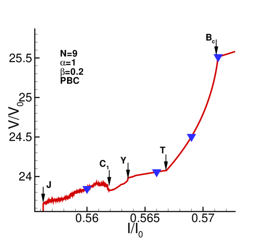
Figure 1: (Color online) The BPR part of the outermost branch for the stack with 9 IJJ at $\alpha=1$, $\beta=0.2$ and periodic boundary conditions. The symbol $\nabla$ indicates the points at which the time dependence of the phase difference and the charge on the layer are investigated.

2 Phase-charge diagrams

The BPR part of the outermost branch of CVC for the stack with 9 IJJ at $\alpha=1$ and $\beta=0.2$ and periodic boundary conditions is presented in Fig. 1. It indicates the current values, at which we have investigated the phase-charge diagrams. The phase-charge diagram is a trajectory of junction in its phase space:($\varphi,Q$). We suggest to use this diagrams as a tool to probe the dynamics of system. For periodic systems like simple harmonic oscillator, the phase portraits in ($\varphi$,$\dot{\varphi}$) space are circles with their centers at the origin of coordinate system. For the system of IJJ it is natural to investigate the phase-charge diagrams.

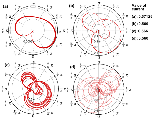
Figure 2: (Color online) The phase-charge diagram (the charge on the first superconducting layer versus the phase difference in the first junction) at different value of bias current. The radial axis is a charge, the azimuthal axis is a phase difference.

Fig. 2 shows such phase-charge diagrams: the variation in time of the modular of charge on the first superconducting layer $Q_{1}$ and phase difference $\varphi_{1}$ in the first Josephson junction of the stack. In these figures the radial axis shows the charge $Q_{1}$ and azimuthal is the phase $\varphi_{1}$.

The beginning part of BPR corresponds to the onset of the parametric resonance: charge on layers is growing. In this region, particularly, $I=0.57126$ (Fig. 2a) the Josephson frequency is still high than LPW frequency, so the trajectory in phase-charge space has some small thickness. At $I=0.569$ (see Fig. 2b) the conditions $\omega_{J}=2\omega_{LPW}$ is practically ideally fulfilled, charge on layers has reached its maximum amplitude, and thickness of trajectory in phase-charge space is just thickness of line. Results of FFT analysis (not presented here) show that at this value of current we observe the peaks corresponding to the LPW only and Josephson frequency does not manifests itself. The system follows this trajectory all time. As we show below, the results of analysis of autocorrelation function, presented in Fig. 3 confirm this interpretation [6].

At $I=0.566$ (Fig. 2c) the trajectory in phase-charge space is wide again. The resonance is passed: $\omega_{J}>2\omega_{LPW}$. Here the amplitude of charge on the layers is merely constant but there is a beating of LPW in the stack. A new large period of system appears [7], but the system after some cycles repeats the same trajectory. Analysis of charge correlations shows that the behavior of system is regular, while Fig. 2d corresponds to a chaotic behavior of the system.

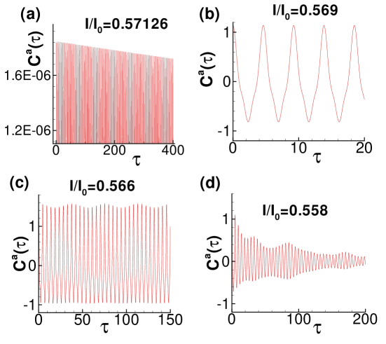
Figure 3: (Color online) The charge autocorrelation function $C^{a}$ for the first layer at different values of bias current in the breakpoint region.

There is a correspondence between phase-charge diagrams and autocorrelation functions, presented in Fig.3. The smallest value of $\tau=\tau_{0}$ with $C^{a}(\tau=\tau_{0})=C^{a}(\tau=0)$ is a period of system. If the autocorrelation function has not such points, then the trajectory of system in phase-charge diagram is open. There is such $\tau=\tau_{0}$ in the cases presented in Figs. 3b and  3c which satisfies the mentioned condition and that’s why in Figs 2b and 2c the trajectories in phase space are closed. But in Fig. 3d the autocorrelation function doesn’t show such $\tau_{0}$ and hence Fig. 2d show open trajectories. Behavior of the system in this case is chaotic. As we mentioned above the thickness of trajectory in Fig.3a is related to the growing charge on the superconducting layers and this is a reason of the amplitude’s decreasing of autocorrelation function with time. Note that to show the very small decreasing of autocorrelation we zoomed the region in vertical axis of Fig.3a. The value $\tau$ is introduced in the definition of autocorrelation function

$$C^{a}_{l}({\tau})=\lim_{(Tf-Ti)\rightarrow\infty}\frac{1}{Tm-Ti}\int_{Ti}^{T_{m}}{Q_{l}(t-\tau)Q_{l}(t)dt}$$ (2)

$C^{a}(\tau=0)$ is a maximum and its value is $C^{a}_{l}(\tau=0)=<Q^{2}_{l}(t)>$. At $I=0.566$ (Fig. 2c) the trajectory in phase-charge space is wide again. The resonance is passed: $\omega_{J}>2\omega_{LPW}$. Here the amplitude of charge on the layers is merely constant.

3 Summary

We found that the phase-charge diagram reflects the dynamical behavior of IJJ. It was shown that the results of the phase-charge diagram analysis are in agreement with the results of the autocorrelation function analysis. We demonstrated that using the phase-charge diagrams (phase portraits) give us a powerful method for investigation of the fine structure in the CVC.

We thank M.R. Kolahchi for his fruitful discussions.

References

References

- [1] Yu. M. Shukrinov, F. Mahfouzi, Supercond. Sci.Technol., 19, S38-S42 (2007).
- [2] Yu. M. Shukrinov, F. Mahfouzi, Phys.Rev.Lett. 98, 157001 (2007).
- [3] Yu. M. Shukrinov, F. Mahfouzi, N. F. Pedersen, Phys. Rev. B 75, 104508 (2007).
- [4] Yu. M. Shukrinov, F. Mahfouzi, and P. Seidel, Physica C 449, 62 (2006).
- [5] T. Koyama and M. Tachiki, Phys. Rev. B 54, 16183 (1996).
- [6] Yu. M. Shukrinov, M. Hamdipour, M. Kolahchi, Phys.Rev.B,80, 014512 (2009).
- [7] Yu. M. Shukrinov, F. Mahfouzi, M. Suzuki, Phys. Rev. B 78, 134521 (2008).