Condensed Groundstates of Frustrated Bose-Hubbard Models

Abstract

We study theoretically the groundstates of two-dimensional Bose-Hubbard models which are frustrated by gauge fields. Motivated by recent proposals for the implementation of optically induced gauge potentials, we focus on the situation in which the imposed gauge fields give rise to a pattern of staggered fluxes, of magnitude $\alpha$ and alternating in sign along one of the principal axes. For $\alpha=1/2$ this model is equivalent to the case of uniform flux per plaquette $n_{\phi}=1/2$, which, in the hard-core limit, realizes the “fully frustrated” spin-1/2 XY model. We show that the mean-field groundstates of this frustrated Bose-Hubbard model typically break translational symmetry. We introduce a general numerical technique to detect broken symmetry condensates in exact diagonalization studies. Using this technique we show that, for all cases studied, the groundstate of the Bose-Hubbard model with staggered flux $\alpha$ is condensed, and we obtain quantitative determinations of the condensate fraction. We discuss the experimental consequences of our results. In particular, we explain the meaning of gauge-invariance in ultracold atom systems subject to optically induced gauge potentials, and show how the ability to imprint phase patterns prior to expansion can allow very useful additional information to be extracted from expansion images.

I Introduction

One of the most striking aspects of the physics of Bose-Einstein condensed systems is their response to rotation. The rotation plays the role of a uniform magnetic field, which frustrates the uniform condensate, forcing it into a state containing quantized vortices and carrying non-vanishing currents.Bloch et al. (2008); Fetter (2009); Cooper (2008) Theory shows that at sufficiently high vortex density this frustration can lead to the breakdown of Bose-Einstein condensation, and the formation of a series of strongly correlated quantum phases which can be viewed as bosonic analogues of the fractional quantum Hall states.Cooper (2008)

In typical magnetically trapped Bose gasesSchweikhard et al. (2004) practical limitations on the rotation rate (vortex density) are such that strongly correlated phases are expected only at a very low particle density where the interaction energy scale is very small.Cooper (2008) As a result, it has proved difficult to reach this strongly correlated regime. (However, see Ref. Gemelke et al., 2010 for interesting recent results for systems with small particle numbers.)

It has been proposed that one can exploit the strong interactions that are available in systems of bosonic atoms confined to optical latticesBloch et al. (2008) to enhance the possibility of achieving these correlated phases. In this context, the natural model to consider is the Bose-Hubbard model with uniform effective magnetic flux [Eq. (II)]. This “frustrated” Bose-Hubbard model can show very interesting physics, far beyond the physics of the usual Bose-Hubbard model.Fisher et al. (1989) Atomic systems well-described by this frustrated Bose-Hubbard have been studied experimentally by using rotating optical lattices,Tung et al. (2006); Williams et al. (2010) albeit so far limited to situations of large lattice constants and large numbers of particles per lattice site which are outside the strongly correlated regime. However, a series of theoretical proposalsJaksch and Zoller (2003); Mueller (2004); Sørensen et al. (2005); Palmer and Jaksch (2006); Palmer et al. (2008); Hafezi et al. (2007); Gerbier and Dalibard (2010) indicate that it should be possible to imprint strong gauge fields on an optical lattice, and thereby realize a regime where interactions are strong, and with both the particle number per site, $n$, and vortex number per plaquette, $n_{\phi}$, of order one. In this regime, theory shows that there are strongly correlated phases representative of the continuum quantum Hall states limitSørensen et al. (2005); Hafezi et al. (2007, 2008) as well as related interesting strongly correlated phases that are stabilized by the lattice itself.Möller and Cooper (2009) Other candidates are related to Mott physics.Umucalilar and Mueller (2010); Powell et al. (2010a)

Our confidence in the existence of strongly correlated phases of the frustrated Bose-Hubbard model relies on the results of large-scale numerical exact diagonalization studies.Sørensen et al. (2005); Hafezi et al. (2007, 2008); Möller and Cooper (2009) However, these studies have found evidence for strongly correlated phases only in a relatively small region of parameter space (spanned by the particle density per site $n$, flux per plaquette $n_{\phi}$, and interaction strength $U/J$). There are surely competing condensed phases, which can be viewed as vortex lattices that are pinned by the lattice.Durić and Lee (2010) An important question emerges from the point of view of these numerical approaches: How does one determine condensation in exact diagonalization studies? In conventional condensed systems, one looks for the maximum eigenvalue of the single particle density matrix of the groundstate.Yang et al. (1993) However, here the condensed states are (pinned) vortex lattices, and therefore break translational symmetry. As a result, one expects a degeneracy of the spectrum in the thermodynamic limit.Cooper et al. (2001); Cooper (2008) How does one quantify the degree of condensation?

In this paper we propose a powerful general numerical method that can be used to identify and characterize condensed groundstates which break a symmetry of the Hamiltonian. We use this to study several cases of interest in the context of optically induced gauge potentials.Dalibard et al. (2010) Optically induced gauge potentials have recently been implemented experimentally without an optical lattice.Lin et al. (2009a, b) These successes encourage a high degree of optimism that the related schemes on optical latticesJaksch and Zoller (2003); Gerbier and Dalibard (2010) will also be successful.

Motivated by the proposals of Jaksch and ZollerJaksch and Zoller (2003) and Gerbier and Dalibard,Gerbier and Dalibard (2010) in this paper we focus not on the case of a uniform magnetic field, but on the case of a two-dimensional square lattice with a staggered magnetic field, with a flux per plaquette of magnitude $\alpha$ that alternates in sign along one of the principal axes. This flux configuration involves much a simpler experimental implementation than the case of uniform flux. As described below, for the special case of $\alpha=1/2$ this is equivalent to the uniform flux. In this case, the model simulates a quantum version of the “fully frustrated” XY model. For other values of $\alpha$, it represents a class of frustrated quantum spin models. Related but different staggered flux Hamiltonians can be generated by time-dependent lattice potentials as discussed in Ref. Lim et al., 2008.

Based on numerical exact diagonalizations, we provide evidence showing that the groundstate breaks translational invariance, and is condensed for all flux densities and (repulsive) interaction strengths. We evaluate the condensate fraction and condensate wavefunctions from the exact diagonalization results. We describe how evidence for translational symmetry breaking can be found in measurements of the real-space and momentum space (expansion) profiles, and how these can be used to determine the condensate depletion. As part of this work, we explain some important general aspects of expansion imaging of systems involving optically induced gauge potentials.

II Model

We shall study the properties of the two-dimensional Bose-Hubbard model subject to an abelian gauge potential, as described by the Hamiltonian

$$\hat{H} = -J\sum_{\langle i,j\rangle}\left[\hat{a}_{i}^{\dagger}\hat{a}_{j}e^{iA_{ij}}+\hat{a}_{j}^{\dagger}\hat{a}_{i}e^{iA_{ji}}\right]+\frac{U}{2}\sum_{i}\hat{n}_{i}(\hat{n}_{i}-1)$$

The operator $\hat{a}_{i}^{({\dagger})}$ destroys (creates) a boson on the lattice site $i$, which we choose to form a square lattice; $U$ describes the onsite repulsion ($U\geq 0$ is assumed throughout); $J$ is the nearest-neighbour tunneling energy. The Hamiltonian conserves the total number of bosons, $\hat{N}=\sum_{i}\hat{n}_{i}=\sum_{i}\hat{a}^{\dagger}_{i}\hat{a}_{i}$. Throughout this work, we shall consider the system to be uniform, with $N$ chosen such that the mean particle density per lattice site is $n$. The results of these studies can be used within the local density approximation to model experimental systems which have an additional trapping potential.

The fields $A_{ij}$ (which satisfy $A_{ij}=-A_{ji}$) describe the imposed gauge potential. All of the physics of the system defined by the Hamiltonian (II) (energy spectrum, response functions, etc.) is gauge-invariant. Therefore, its properties depend only on the fluxes through plaquettes

$$n^{a}_{\phi}\equiv\frac{1}{2\pi}\sum_{i,j\in a}A_{ij}$$ (1)

where $a$ labels the plaquette, and the sum represents the directed sum of the gauge fields around that plaquette (the discrete version of the line integral), as illustrated in Fig. 1(a).

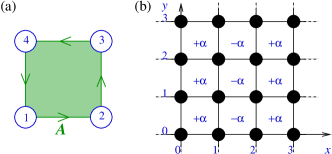
Figure 1: (a) The gauge-invariant flux through the plaquette, $n_{\phi}$, is defined by $n_{\phi}\equiv\frac{1}{2\pi}\sum_{i,j}A_{ij}=\frac{1}{2\pi}\left(A_{12}+A_{23}+A_{34}+A_{41}\right)$ (b) The simplest optically induced gauge potential to imprint on the square latticeJaksch and Zoller (2003); Gerbier and Dalibard (2010) has an alternating pattern of fluxes of magnitude $\alpha$, Eq. (6).

Since each phase $A_{ij}$ is defined modulo $2\pi$, the gauge invariant fluxes (1) are defined modulo $1$ (i.e. are invariant under $n_{\phi}^{a}\to n_{\phi}^{a}+1$), so they can be restricted to the interval $-1/2<n^{a}_{\phi}\leq 1/2$.

The gauge-invariant fluxes through the plaquettes lead to an intrinsic “frustration” of condensed (superfluid) phases on the Bose-Hubbard system. This is best understood in the case of strong interactions, $U\gg J$, where double occupancy is excluded. In this hard-core limit, the Bose-Hubbard model is equivalent to a spin-1/2 quantum magnet, using the standard mapping $\hat{s}_{i}^{z}=\hat{n}_{i}-\frac{1}{2}$, $\hat{s}_{i}^{+}=\hat{a}_{i}^{\dagger}$, $\hat{s}_{i}^{-}=\hat{a}_{i}$, with Hamiltonian (up to a constant shift in energy)

$$\hat{H}_{\rm h-c} = -J\sum_{\langle i,j\rangle}\left[\hat{s}_{i}^{+}\hat{s}^{-}_{j}e^{iA_{ij}}+\hat{s}_{j}^{+}\hat{s}^{-}_{i}e^{-iA_{ij}}\right]$$ (2)

(The conservation of particle number becomes conservation of $\hat{S}^{z}=\sum_{i}\hat{s}^{z}_{i}=\hat{N}-1/2$.) This Hamiltonian describes a quantum spin-1/2 magnet, experiencing XY nearest neighbour spin exchange interactions. These exchange interactions are “frustrated” by the gauge fields. The “frustration” can be seen by considering the natural mean-field limit of the spin Hamiltonian (2), generalizing from spin-$1/2$ to spin-$S$ and taking the $S\to\infty$ limit.Durić and Lee (2010) Then, the (vector of) spin operators $\hat{s}_{i}$ can be replaced by the classical vector $\vec{s}$ of fixed length $S$. It is convenient to parameterize this vector as

$$\vec{s}=S(\sin\theta\cos\phi,\sin\theta\cos\phi,\cos\theta)$$ (3)

which represents the spin by the polar and azimuthal angles $\theta,\phi$. The Hamiltonian becomes the (classical) energy functional

$$H_{\rm mft}=-2JS^{2}\sum_{\langle i,j\rangle}\sin\theta_{i}\sin\theta_{j}\cos(\phi_{i}-\phi_{j}+A_{ij})$$ (4)

and it is natural define the fractional occupation of the lattice sites by $n_{i}=(1/2)(1+\cos\theta_{i})$.

The restricted space of configurations with $\theta_{i}=\pi/2$ is important for groundstate configurations with (uniform) density $n=1/2$. In this case, $s_{z}=0$, so all spins lie in the $x$-$y$-plane and the Hamiltonian becomes that of the frustrated XY model.Teitel and Jayaprakash (1983) Here, “frustration” refers to the fact that, with $n_{\phi}\neq 0$ for any plaquette, the angles $\phi_{i}$ around this plaquette cannot be chosen in order to maximally satisfy the XY exchange couplings. This is illustrated in Fig. 2.

       

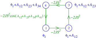
Figure 2: Illustration of the frustrated coupling of the XY spin model around a plaquette with non-zero flux $n_{\phi}$. For a given phase $\phi_{1}$ at site 1, one can choose $\phi_{2}$, $\phi_{3}$, and $\phi_{4}$ to maximally reduce the energy on three of the bonds (with a contribution of $-JS^{2}$ to the energy for each). However, the exchange energy on the remaining bond is $-JS^{2}\cos(A_{12}+A_{23}+A_{34}+A_{41})=-JS^{2}\cos(2\pi n_{\phi})$. For $n_{\phi}\neq 0$, this bond cannot also be fully satisfied, indicating the magnetic frustration. Maximal frustration occurs for $n_{\phi}=1/2$.

Maximal frustration occurs for $n_{\phi}=1/2$. This situation is referred to as the “fully frustrated” case. The “fully frustrated” classical XY model has been much studied as an interesting frustrated classical magnet with a non-standard thermal phase transition.Villain (1977) The frustrated Bose-Hubbard model that we study here is a class of frustrated spin-$1/2$ quantum systems that are analogous to this frustrated classical model. We shall focus on the nature of the groundstates of the system.

III Staggered Fluxes

Motivated by proposals for optically induced gauge potentials,Jaksch and Zoller (2003); Gerbier and Dalibard (2010) we consider a situation in which the flux is staggered in the $x$ direction. Specifically, we choose the gauge (and geometry) described in Ref. Gerbier and Dalibard, 2010, for which

$$A_{ij}=2\pi\alpha\,y_{i}(x_{i}-x_{j})\times(-1)^{x_{i}}$$ (5)

where $(x_{i},y_{i})$ is the pair of integers that define the position of lattice site $i$ (i.e. the cartesian co-ordinates position in units of the lattice constants, $a_{x}$, $a_{y}$, in the $x$- and $y$-directions, as shown in Fig.1(b)). Since the lattice is square with nearest-neighbour hopping, this has the effect that hopping in the $y$ direction has no gauge field ($A_{ij}=0$) while hopping in the $x$ direction involves a phase $A_{ij}=2\pi\alpha y_{i}(-1)^{x_{i}}$ that alternates from one row to the next. The magnitude of the flux per plaquette is

$$n^{a}_{\phi}=(-1)^{x_{a}}\alpha\,,$$ (6)

where the position $x_{a}$ is defined by the $x$-position of the “bottom-left” corner of the plaquette (i.e. the minimum $x_{i}$ for all sites $i$ surrounding the plaquette $a$). The flux is staggered in the $x$-direction, as shown in Fig. 1(b).

A special situation arises for $\alpha=1/2$. Then, the case of alternating fluxes of $n^{a}_{\phi}=(-1)^{x_{a}}\frac{1}{2}$ is gauge-equivalent to that of uniform flux $n^{a}_{\phi}=\frac{1}{2}$. The (gauge-invariant) properties of this case have higher translational symmetry than the case of $\alpha\neq 0,1/2$. Furthermore, a gauge can be chosen in which $e^{iA_{ij}}$ is real, meaning that the Hamiltonian is time-reversal symmetric. Indeed the gauge (5) has this property. While gauge invariance allows the physics of (II) to be studied in any gauge, as we shall describe below, the expansion images of the atomic gas are gauge-dependent. We shall therefore be clear to specify the gauge considered.

Under the conditions that we study, significant insight into the physics of the frustrated Bose-Hubbard model can be obtained by studying its properties within mean-field theory. Indeed, one important goal of this work is to show how the mean-field groundstates emerge from the results of exact diagonalization studies.

III.1 Single Particle Spectrum

We first ignore interactions, and study the single particle energy eigenstates. For the gauge field we consider (5), the unit cell can be chosen to have size $2\times 1$ (in the $x$- and $y$-directions), and the energy eigenstates are then

$$\psi_{i}=e^{i(k_{x}x_{i}+k_{y}y_{i})}\times\left\{\begin{array}[]{l}\psi_{e}\quad\quad\quad\quad x_{i}\;\mbox{even}\\ \psi_{o}e^{i2\pi\alpha y_{i}}\quad x_{i}\;\mbox{odd}\end{array}\right.$$ (7)

with the momenta in the ranges $-\pi/2\leq k_{x}<\pi/2$ and $-\pi\leq k_{y}<\pi$. [We express $k_{x}$ and $k_{y}$ in units of $1/a_{x}$ and $1/a_{y}$ respectively.] The energy eigenvalues $E$ and eigenfunctions within the unit cell, $(\psi_{e},\psi_{o})$, follow from

$$-2J\left(\begin{array}[]{cc}\cos(k_{y})&\cos(k_{x})\\ \cos(k_{x})&\cos(k_{y}+2\pi\alpha)\end{array}\right)\left(\begin{array}[]{c}\psi_{e}\\ \psi_{o}\end{array}\right)=E\left(\begin{array}[]{c}\psi_{e}\\ \psi_{o}\end{array}\right)$$ (8)

The lowest energy state has $k_{x}=0$. For $\alpha<\frac{1}{\pi}\arccos\left((\sqrt{5}-1)/2\right)\simeq 0.288$, there is a single minimum at $k_{y}=\pi\alpha$. However, for $\alpha>0.288$ this minimum splits in two, and there are two degenerate minima defining single particle states $\psi^{A}_{i}$ and $\psi^{B}_{i}$. The wavevectors of these states, $k_{y}^{A,B}$ are shown in Fig. 3. They are related by $k^{A}_{y}+k_{y}^{B}=-2\pi\alpha$. Hence $\cos(k^{A/B}_{y})=\cos(k^{B/A}_{y}+2\pi\alpha)$, so the Hamiltonian (8) is the same for both states provided the two sites of the unit cell are swapped. Therefore, $\psi^{A}$ and $\psi^{B}$ are exactly degenerate, and their wavefunctions related by $\psi^{A}_{e/o}=\psi^{B}_{o/e}$.

Figure 3: The single-particle groundstate is non-degenerate for $\alpha<0.289$, but is two-fold degenerate for $\alpha>0.289$. The two minima are at wavevectors $k^{A}_{y},k^{B}_{y}$ shown above (both have $k_{x}=0$).

The appearance of two degenerate minima in the single-particle spectrum leads to the question of whether the groundstate is a “simple” condensate, or “fragmented”.Mueller et al. (2006) Following the general result,Griffin et al. (1996) one expects that weak repulsive interactions will lead to a simple condensate in which all particles condense the same single particle state. The nature of this condensate can depend on the properties of the two states, and the nature of the interactions. However, if the condensate wavefunction contains non-zero weights of both states, with wavevectors $k_{y}^{A}$ and $k_{y}^{B}$, then the condensate breaks translational symmetry in the $y$ direction.

Similar physics – of a two-component Bose gas – has been discussed recently in the context of optically induced gauge potentials in the continuum.Spielman (2010); Ho and Zhang (2010); Wang et al. (2010) For the case we consider, one principle difference is that there is an underlying lattice periodicity. Phases with broken translational symmetry can therefore “lock” to the lattice periodicity, leading to condensed groundstates with a broken discrete translational symmetry. Furthermore, the unit cells of the phases that we describe contain particle currents, which can be viewed as arrays of vortices and antivortices.

In the following we shall explore the nature of this symmetry breaking. A principle result will be to show that the results of exact diagonalization studies are consistent with simple condensation in a symmetry broken state. We shall focus on two cases:

(i) $\alpha=1/2$. Here, the model is equivalent to the case of uniform fluxes $n_{\phi}^{a}=1/2$. The (gauge-invariant) system therefore enjoys the full translational symmetry of the lattice. The minima are spaced by $\Delta k_{y}=\pi$, suggesting that the broken symmetry state will have translational period $2$ in the $y$-direction. The symmetry broken state will have two degenerate configurations.

(ii) $\alpha=\frac{1}{\pi}\arccos\left(\frac{1}{2}\sqrt{\frac{1}{2}(9-\sqrt{65})}\right)\simeq 0.389$. This value is chosen such that $\Delta k_{y}=2\pi/3$, such that the broken translational symmetry state has period $3$ in the $y$-direction. The symmetry broken state will have three degenerate configurations.

Throughout this work, we concentrate on cases where the particle density $n$ is non-integer. Thus, we do not discuss the properties of the Mott insulator states. While frustration by the gauge fields can affect the stability of the Mott insulating states,Umucalilar and Oktel (2007); Goldbaum and Mueller (2008) the qualitative form of these insulating states is unchanged. We focus on the nature of the superfluid states, the properties of which are much changed in the presence of the frustrating gauge fields.

III.2 Gross-Pitaevskii Theory

One can understand the effects of weak interactions, i.e. $U\ll nJ$, within Gross-Pitaevskii mean-field theory. One assumes complete condensation, forming a many-body state

$$|\Psi_{c}\rangle\equiv\left(\sum_{i}\psi^{c}_{i}\hat{a}^{\dagger}_{i}\right)^{N}|0\rangle$$ (9)

where $\psi^{c}_{i}$ is the (normalized) condensate wavefunction. The condensate wavefunction is determined by viewing (9) as a variational state, and minimizing the average energy per particle

$$\frac{\langle\hat{H}\rangle}{N} = -J\sum_{\langle i,j\rangle}\left[\psi^{c*}_{i}\psi^{c}_{j}e^{iA_{ij}}+\psi^{c*}_{j}\psi^{c}_{i}e^{iA_{ji}}\right]$$ (11)

$$+\frac{U}{2}(N-1)\sum_{i}|\psi^{c}_{i}|^{4}-\frac{U}{2N}$$

For large systems $N\gg 1$ the typical interaction energy (11) is of the order of $Un$, while the kinetic energy (11) is of order $J$.

In the weak coupling limit, $nU\ll J$, the groundstates of the Gross-Pitaevskii equation can be obtained by assuming that the condensate consists only of those states that minimize the single-particle kinetic energy. For $\alpha<\alpha_{c}$, there is a single minimum, so the condensate will be formed from this state alone. For $\alpha>\alpha_{c}$, there are two degenerate minima, and we should write

$$\psi^{c}=A\psi_{k_{A}}+B\psi_{k_{B}}$$ (12)

which (schematically) denotes a linear superposition of the states in these two minima. Then one chooses $A$ and $B$ to minimize the interaction energy $\sum_{i}|\psi^{c}_{i}|^{4}$.

III.2.1 The case $\alpha=1/2$

This is the case of the fully frustrated Bose-Hubbard model, $\alpha=1/2$, which is gauge equivalent to uniform plaquette fluxes of $n_{\phi}=1/2$. Minimizing the interaction energy within states of the form (12) leads to two solutions which we can denote schematically by

$$\psi^{c}_{\pm}=\frac{1}{\sqrt{2}}\left[\psi_{k_{A}}\pm i\psi_{k_{B}}\right]$$ (13)

In detail, the wavefunctions are

$$\psi^{c}_{\pm,i}=\frac{1}{2\sqrt{2-\sqrt{2}}}\times\left\{\begin{array}[]{l}1\pm i(\sqrt{2}-1)(-1)^{y_{i}}\quad\quad x_{i}\;\mbox{even}\\ (\sqrt{2}-1)(-1)^{y_{i}}\pm i\quad\quad\quad x_{i}\;\mbox{odd}\end{array}\right.$$ (14)

where $i$ refers to the labelling in Fig. 2. The wavefunctions are illustrated in Fig. 4. The pattern of phases is equivalent to that of the ordered groundstate of the fully-frustrated classical XY modelVillain (1977).

Since the condensed state is a superposition of states with different $k_{y}$, it is a state with broken translational invariance. The difference in wavevectors is $\Delta k_{y}=k_{y}^{A}-k_{y}^{B}=\pi$, so the new unit cell in the $y$-direction has size $\Delta y=2$ (in units of the lattice constant $a_{y}$).

It is useful to recall that the Hamiltonian at $\alpha=1/2$ is time-reversal invariant, so all of its eigenvectors can be chosen real. The fact that the condensed wavefunctions (14) are imaginary shows that these break time-reversal symmetry. The two states are time-reversed partners, $\psi^{c}_{\pm}=\left(\psi^{c}_{\mp}\right)^{*}$.

The two states are the two (time-reversed) partners of a so-called “staggered flux” phase, a related version of which has been discussed in the context of the cuprate superconductors.Affleck and Marston (1988) This phase is characterised by circulating currents around the plaquettes, which are arranged in a staggered “checkerboard” pattern. It is straightforward to show that the states $\psi^{c}_{\pm}$ do carry these staggered gauge-invariant currents.

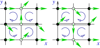
Figure 4: Illustration of the two (degenerate) mean-field groundstates of the fully frustrated model, $n_{\phi}=1/2$. The arrows on each lattice site represent the phase of the condensate wavefunction (the amplitude is constant). The two phases are characterized by staggered circulating currents, in directions illustrated within the plaquettes. Double lines mark links where a ‘phase’ $e^{i\pi}$ is imprinted.

We emphasize that the underlying Hamiltonian is both translationally invariant and time-reversal invariant, so the emergence of these staggered flux states is a result of the breaking of both of these symmetries.

The same condensed states have been shown to describe the groundstates of a related Bose-Hubbard model.Lim et al. (2008) In constrast to the model that we study, in the model of Ref. Lim et al., 2008, the staggered flux $\alpha$ is applied directly in a checkerboard pattern. However, for staggered flux of $\alpha=1/2$ the two models coincide (up to a choice of gauge, as described below).

The derivation of the states (13) described above was presented in the weak-coupling limit, $nU\ll J$. However, note that the state has the special property that the density is uniform $|\psi_{i}^{c}|^{2}=\mbox{constant}$. Therefore, these condensates already minimize the interaction energy $\sum_{i}|\psi_{i}^{c}|^{4}$ at fixed average density. With increasing interaction strength $nU\sim J$, the condensate does not change. (We have confirmed this with extensive numerical simulations of the mean-field theory.) Even in the regime $U\gg J$ where Gross-Pitaevskii theory becomes unreliable owing to the suppression of number fluctuations and a Gutzwiller mean-field theory is required, the condensate wavefunction remains the same.

III.2.2 The case $\alpha=0.389$

Choosing $\alpha=\frac{1}{\pi}\arccos\left(\frac{1}{2}\sqrt{\frac{1}{2}(9-\sqrt{65})}\right)\simeq 0.389$ leads to the situation in which $\Delta k_{y}=2\pi/3$. Then, a state of the form (12) with non-zero $A$ and $B$ breaks translational symmetry with a period of $\Delta y=3$ in the $y$-direction.

Minimizing the interaction energy over states of the form (12) leads to the conclusion that the optimum condensate wavefunction is the superposition

$$\psi^{c}_{\pm}=\frac{1}{\sqrt{2}}\left[\psi_{k_{A}}+e^{i\chi}\psi_{k_{B}}\right].$$ (15)

Thus, the condensate does break translational symmetry, with the expected period of $\Delta y=3$. Unlike the (special) case of $\alpha=1/2$, for these functions the density is not uniform, so spatial patterns of the density show this periodicity.

One interesting feature of this mean-field result is that the interaction energy is independent of the phase $\chi$ appearing in (15). Thus, there is an infinite set of condensed groundstates, which are related by the different choices of the phase $\chi$. In a continuum model, this infinite degeneracy would correspond to the broken continuous translational symmetry, the different choices of $\chi$ denoting translations of the same state. Here the model is explicitly defined on a lattice, so there is no continuous translational symmetry. Since the wavefunction is defined only on lattice sites, the states with different values of $\chi$ are not just related by simple translations. Nevertheless, for weak interactions $nU\ll J$, we find that, surprisingly, there emerges a continuous degeneracy, beyond the expected threefold degeneracy from translations. This gives an additional “Goldstone” mode, associated with slow spatial variations of $\chi$ as a function of position. (The same feature arises for values of $\alpha$ for which $\Delta k_{y}=2\pi/p$ with $p\neq 2$.)

Since this additional emergent degeneracy is not protected by a symmetry of the Hamiltonian, one does not expect it to survive in general (e.g. to stronger interactions or to quantum fluctuations). Indeed, we find that by performing mean-field theory to stronger interaction strengths, the continuous degeneracy is lost. Including energy corrections to order $(nU)^{2}/J$ we find that the three cases $\chi=0,\pm 2\pi/3$ are selected as the energy minima. This gives rise to a set of three degenerate groundstates, with a unit cell of size $\Delta y=3$ and all related by translations in the $y$ direction. The Goldstone mode described above develops a gap.

III.2.3 The case of general $\alpha$

For typical cases of $\alpha$ in the range $\alpha_{c}<\alpha<1/2$, there are two minima in the single particle energy spectrum, but the spacing $\Delta k_{y}$ is incommensurate with the underlying lattice. In the weak coupling limit $nU\ll J$, one expects the groundstate to remain incommensurate with the lattice, having a continuous degeneracy (along the lines of that described by the phase $\chi$ above). However, for sufficiently strong interactions, the density wave will “lock” to the lattice, via an incommensurate-commensurate phase transition.Pokrovsky and Talapov (1979) Additionally, for staggered flux $\alpha\gtrsim\alpha_{c}$, near the bifurcation in Fig. 3, the single-particle dispersion becomes very flat, and we expect a regime of large fluctuations where potential condensate groundstates will be strongly depleted.

IV Numerical Methods

In order to investigate the quantum groundstate of the frustrated Bose-Hubbard model, we have performed large scale exact diagonalization studies of the model (II). We define the system on a square lattice of $N_{s}=L_{x}\times L_{y}$ sites, and impose periodic boundary conditions to minimize finite size effects. For a total number of bosons, $N$, we therefore study a system with mean density $n=N/(L_{x}L_{y})$.

The possible geometries and system sizes are constrained by the form of the gauge potential that is applied. Furthermore, the plaquette fluxes determine the translational symmetries of the Hamiltonian, and hence the conserved momenta. For staggered flux (6), in the general case ($\alpha\neq 0,1/2$) the translational symmetries are those of the unit cell with size $2\times 1$ (in $x$ and $y$ directions). Higher symmetry arises for the cases $\alpha=0$ and $\alpha=1/2$, for which the flux is uniform; in the latter case, the (magnetic) translational symmetries of many-particle systems follow from Ref. Kol and Read, 1993.

By definition, the Hamiltonian commutes with the unitary transformations that effect these translational symmetries. The energy eigenstates are therefore also eigenstates of these translational symmetry operators (i.e. eigenstates of conserved lattice momentum). In any exact numerical calculation, the energy eigenvectors will also be eigenstates of the conserved lattice momentum. However, as described above, in general the mean-field states break the translational symmetry. Thus the mean-field states are not eigenstates of momentum. In order to make comparisons with the mean-field states, and the possibility of condensation, one must allow for this breaking of translational symmetry.

IV.1 Condensate Fraction

Often the groundstates of (repulsive) interacting bosons can be understood in terms of Bose-Einstein condensation. Interactions between the particles lead to depletion of the condensate. If the effects of interactions are very strong, these may even drive a phase transition from the condensed phase into non-condensed phases. It is therefore very important to know if the groundstate remains condensed. (If not, then the system may be described by a novel, uncondensed, and possibly strongly correlated phase of matter.)

The condensate fraction is quantified by the general definition introduced by Yang.Yang et al. (1993) From the many-particle groundstate $|\Psi_{0}\rangle$, one forms the single particle density operator

$$\rho_{ij}=\langle\Psi_{0}|\hat{a}^{\dagger}_{i}\hat{a}_{j}|\Psi_{0}\rangle\,,$$ (16)

a Hermitian operator, the trace of which $\sum_{i}\rho_{ii}$ is the mean (total) number of particles, $N$. Then, one finds the eigenvalues of $\rho_{ij}$. For “simple” BECs,Leggett (2001) the spectrum has one eigenvalue which is of order $N$,Yang et al. (1993) and which is therefore much larger than all others for large $N$ (the thermodynamic limit). Denoting this largest eigenvalue $\lambda_{0}$, the condensate density $n_{c}$ and condensate fraction $x_{c}$ for average density $n$ are defined byYang et al. (1993)

$$x_{c}\equiv\frac{n_{c}}{n}\equiv\frac{\lambda_{0}}{N}\,.$$ (17)

The eigenvector of $\rho_{ij}$ corresponding to the largest eigenvalue is the condensate wavefunction, $\psi_{i}^{0}$.

While this method is applicable in the simplest of situations, it gives misleading results in cases where the groundstate of the system breaks a symmetry of the Hamiltonian in the thermodynamic limit. In that case it is well known that, for a finite sized system (in which the ground state is an eigenstate of all symmetry operators), an analysis of the density matrix states shows a “fragmented” condensate in which there is more than one eigenvalue of order $N$. (See Ref. Mueller et al., 2006 for a discussion of fragmentation in the context of cold atomic gases.) The origin of this fragmentation, and its relationship to symmetry breaking, is well-understood for simple model systems with no condensate depletion, for example for condensation of $N$ bosons in two orbitals.Mueller et al. (2006); Dagnino et al. (2009) From the practical point of view of exact numerical calculations, it is important to have a prescription for how to quantify the degree of condensation in general – i.e. in cases where there are many degrees of freedom and condensate depletion can be significant.

IV.2 Condensate Fraction with Symmetry Breaking

We propose a method to determine, on the basis of numerical exact diagonalization studies, the condensate fraction in cases where the condensed state breaks a symmetry in the thermodynamic limit. Given the context of this paper, we focus on the case of translational symmetry. The method, however, is very general: no specific knowledge is required of the condensed state, or indeed of the symmetry that is broken. These emerge directly from the numerical calculations in an unbiased way.

The starting point is to determine the energy spectrum, in order to identify if the groundstate may have a broken symmetry in the thermodynamic limit. As ever with numerical studies, one must study the spectrum with varying systems size (up to as large a system size as can be achieved), in order to glean information about the properties of the spectrum in the thermodynamic limit. It is well-known that the signature of (translational) symmetry breaking in a finite size calculation is the appearance of a set of quasi-degenerate energy levels in the spectrum, with different eigenvalues of the conserved quantity associated with the symmetry (i.e. momentum in the case of translational symmetry breaking). In the context of cold atomic gases, this has been illustrated for spin-rotational invariance,Law et al. (1998); Ho and Yip (2000) translational and rotational symmetry breaking,Cooper et al. (2001); Cooper (2008); Zhang et al. (2010) and parity.Parke et al. (2008); Dagnino et al. (2009) In the thermodynamic limit, these states become degenerate, and it becomes valid to superpose the states (e.g. as selected by an arbitrary weak symmetry breaking perturbation). Any superposition of all these states forms a groundstate which has broken symmetry. Before superposition, each of the states (eigenstates of the symmetry operators) can be viewed as fragmented condensates.Mueller et al. (2006)

Based on the results of these calculations of the energy spectrum, one can look to see if, in the thermodynamic limit, several states are tending to become degenerate. The emergence of this degeneracy appears when the system size is sufficiently large; if the degeneracy is not well resolved, then this suggests that the numerical calculations are not on a sufficiently large system size to be conclusive. In many cases, an emergent quasi-degeneracy can be very convincingly established.Cooper et al. (2001); Cooper (2008); Parke et al. (2008); Dagnino et al. (2009) In many practical cases of interest where the degeneracy is not fully established, it can still be of value to make the hypothesis that a small number of low-energy states will be degenerate in the thermodynamic limit, and to test if this hypothesis is borne out by a high condensate fraction.

Suppose that an analysis of the energy spectrum suggests that there are $D$ such states, $|\Psi_{0}^{\mu}\rangle$, with $\mu=1,2,\ldots,D$, which tend towards degeneracy in the thermodynamic limit. We assume that these $D$ states can be distinguished by eigenvalues of symmetry operators (e.g. no two have the same momenta). In order to investigate the possibility of simple BEC in a broken symmetry state, we propose that one forms the superposition state

$$|\Psi^{c}_{0}\rangle\equiv\sum_{\mu=1}^{D}c_{\mu}|\Psi_{0}^{\mu}\rangle$$ (18)

which depends on the $D$ complex amplitudes $c_{\mu}$. Then, for this superposition state – which is not an eigenstate of the (translational) symmetry – one should determine the single particle density matrix (16) and find the condensate fraction (17), each of which are functions of the parameters $c_{\mu}$. We define the condensate fraction of the broken symmetry state by in terms of the optimal choice

$$X_{c}\equiv\max_{c_{\mu}}\left[x_{c}(c_{\mu})\right]\,.$$ (19)

The corresponding optimizing coefficients $c_{\mu}$ define the associated condensate wavefunction (18). Since this is a broken symmetry state, in general there are $D$ sets of coefficients $c_{\mu}$ which give the (same) maximum condensate fraction, and hence $D$ such condensed states. These correspond to the $D$ broken symmetry states, and are related by applications of the symmetry operations.

Below, we illustrate the application of this approach for the cases of the Bose-Hubbard model with staggered flux, at $\alpha=1/2$ (fully frustrated) where $D=2$, and at $\alpha=0.389$ where $D=3$.

IV.3 Unfrustrated Bose-Hubbard Model

As a warm-up, and to test the quantitative validity of exact diagonalization in determining the condensate fraction, we study the Bose-Hubbard model in the absence of gauge fields (all plaquette fluxes vanish, $n^{a}_{\phi}=0$). In this case, for non-integer particle density, it is known that the groundstate is condensed,Fisher et al. (1989) and the condensate fraction has been established by detailed numerical studies including quantum Monte Carlo,Hébert et al. (2001) as well as in spin-wave theory.Bernardet et al. (2002) For $n=1/2$, the condensate fraction is $x_{c}=1$ for $U/J=0$, and falls to $x_{c}\simeq 0.4$ in the hard-core limit $U/J\to\infty$.Bernardet et al. (2002)

We have used ED results on systems of up to $L_{x}\times L_{y}=5\times 6$ to determine the condensate fraction. Consistent with the lack of symmetry breaking, in all cases the spectrum shows a clear groundstate. (The broken gauge invariance of this state will appear in a emergent quasi-degeneracy at different particle numbers. We work at fixed particle number.) By forming the single particle density operator, and finding its maximal eigenvalue, we find that for hard-core bosons at $n=1/2$ the condensate fraction is $0.433(6)$. The favourable comparison with the Monte Carlo result illustrates that, for this case, the system sizes amenable to ED are sufficiently large to allow accurate quantitative determination of $x_{c}$.

IV.4 Fully Frustrated Bose-Hubbard Model, $\alpha=1/2$

We now turn to the case of the fully frustrated Bose-Hubbard model, $\alpha=1/2$, which is gauge equivalent to uniform plaquette fluxes $n_{\phi}=1/2$. To analyse this case, we study system sizes for which the translational symmetryKol and Read (1993) is the largest, implying the largest possible Brillouin zone for the conserved (many-particle) momentum, and no degeneracy associated merely with the magnetic translations. (This is the “preferred” case of $d=1$ in the terminology and notation of Ref. Kol and Read, 1993.)

In these cases, where no many-body degeneracy is expected, the groundstate in the non-interacting system still remains degenerate due to the degeneracy of the single-particle groundstate. This degeneracy is split due to interactions in the system. We find an emerging two-fold quasi-degeneracy in the spectrum for sufficiently large system sizes even in the case of hardcore interactions, as shown in the inset of Fig. 5 (left frame). Following the procedure of §IV.2, we recognize this as a sign of possible symmetry-breaking with $D=2$. We apply the prescription in §IV.2 to determine the maximal condensate fraction.

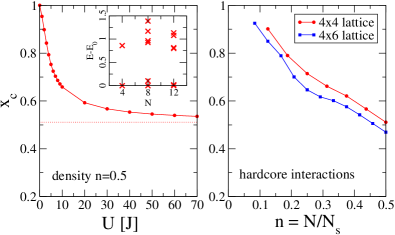
Figure 5: Exact diagonalisation results for the condensate fraction $x_{c}$ for the maximally condensed state at $n_{\phi}=1/2$, i.e. incorporating translational symmetry breaking: as a function of the interaction strength $U$ (left); and as a function of particle density $n$ in the hard-core limit (right). In addition, the inset in the left frame shows the low-lying spectrum of the system for the case of hardcore interactions at half filling. These spectra clearly confirm the emergence of a twofold degenerate groundstate in large systems. At $N=12$, the splitting is barely discernable at the scale of the figure.

In Fig. 5 we present the results of these calculations of the (maximal) condensate fraction for the fully frustrated Bose-Hubbard model, both as a function of $U/J$ for $n=1/2$, and as a function of $n$ in the hard-core limit $U/J\to\infty$. In all cases, we find that the groundstate appears to be fully condensed. The smallest condensate fraction is for $n=1/2$ and $U/J\to\infty$. Here, an extrapolation in $1/N$ to the thermodynamic limit yields a condensate fraction of about $x_{c}\simeq 0.39$. In the graphs of Fig. 5(b) there appears to be a reduction of condensate fraction at about $n\simeq 0.25$. We associate this with the fact that, on the lattice, the Laughlin state of bosons would appear for full frustration $n_{\phi}=1/2$ at density $n=1/2$.Möller and Cooper (2009) Extrapolation of the condensed fraction in this case yields $x_{c}\sim 0.48(2)$. Although the possibility of Laughlin correlations may act to destabilize the condensed state, the groundstate at this density is a condensed (superfluid) phase. In all cases, the nature of the groundstate that we find closely matches the predictions of mean-field theory. First, we can check that symmetry breaking is of the same form. Furthermore, the condensate wavefunction that we obtain is exactly that described above in Eq. (13). As discussed previously, these states have uniform density, which makes them highly robust to details of the interaction potential.

The results provide the first evidence from exact diagonalizations that, under all conditions, the groundstate of the fully frustrated Bose-Hubbard model is condensed. Our model includes the possibility of particle-number fluctuations, and thus goes beyond previous studies using the picture of Josephson-junction arrays that is based on phase fluctuations only.Polini et al. (2005) Furthermore, our results provide a quantitative measure of the condensed fraction.

It is interesting to compare the results to those that would be obtained from a Gutwiller ansatz. In the hard-core limit, the Gutwiller mean-field state has $x_{c}=1-n$. Thus, at $n=1/2$ the Gutzwiller theory predicts a condensate fraction of $0.5$. This is close to the value we obtain from exact diagonalisation results, $\simeq 0.39$, indicating that Gutzwiller theory is quantitatively fairly accurate in this case. At $n=1/4$ the Gutzwiller theory predicts a condensate fraction of $0.75$. The exact diagonalization result of $\simeq 0.48$, shows a large quantitative discrepancy. As described above, we attribute this to the competition introduced by Laughlin-like correlations which act to destabilise the condensate. Another interesting observation can be made by comparing the condensate fractions for the frustrated Bose Hubbard model at $n_{\phi}=1/2$ with the unfrustrated zero-field case. For half filling, the gauge-field reduces the condensate fraction seen in our exact diagonalizations from about $x_{c}(n_{\phi}=0)=0.43$ to $x_{c}(n_{\phi}=1/2)=0.39$. For $n=1/4$ on the other hand, the reduction is more significant, with $x_{c}(n_{\phi}=0)=0.66(1)$ being reduced to $x_{c}(n_{\phi}=1/2)=0.48$ in the presence of the field.

IV.5 Staggered Flux Bose-Hubbard Model, $\alpha=0.389$

This is the staggered flux value at which $\Delta k_{y}=2\pi/3$, so we expect a broken symmetry state with unit cell size $\Delta y=3$, and thus a groundstate degeneracy of $D=3$ in the thermodynamic limit. As described above, this is borne out in mean-field theory, at least for sufficiently strong interactions.

The numerical results are consistent with these expectations. For large interactions, a clear three-fold degeneracy appears in the groundstate. Assuming $D=3$ for all interaction strengths leads to the condensate fraction shown in Fig. 6 for density $n=1/2$. For small $U/J$ and/or density $n$, the results of our analysis show that the groundstate is condensed in the manner predicted by mean-field theory. For the strongest interactions (hard-core interactions and $n=1/2$) finite-size effects remain significant, and it is difficult to be sure that extrapolation to the thermodynamic limit will leave a non-zero condensate fraction (see inset of Fig. 6). In finite size systems, the condensed wavefunction obtained from the numerical procedure is in good qualitative agreement with the results of mean-field theory described above. At very weak interactions, the presence of the Goldstone mode discussed in §III.2.2 is also visible. For $U/J\lesssim 0.1$, the results in Fig. 6 show a discontinuous drop in $x_{c}$. This occurs when the splitting of the three-fold groundstate degeneracy (due to finite size effects) is larger than the energy scale which mean-field theory shows is required to “lock” the density wave to the underlying lattice. Thus, this reduction in $x_{c}$ at small $U/J$ is a finite-size effect. In this regime, we can recover a large condensate fraction, $x_{c}\simeq 1$, by including additional levels ($D>3$) to account for the higher degree of symmetry breaking.

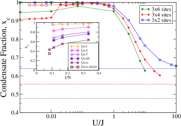
Figure 6: Exact diagonalisation results for the condensate fraction $x_{c}$ as a function of interaction strength $U/J$, for the staggered flux with $\alpha=0.389$ where the groundstate shows three-fold translational symmetry breaking. Results are at half filling, $n=1/2$, calculated for $N=6$ particles on a system of dimensions $L_{x}\times L_{y}=4\times 3$. Small symbols show optimisations over the lowest three eigenstates. For $U/J\lesssim 0.1$ a maximally condensed state requires to also include the low-lying Goldstone modes (large symbols; see main text). The condensate fraction calculated in the hardcore limit is shown as a dashed line. Inset: Scaling of the condensate fraction with system size for different $U$. For the largest system with $N=12$ particles in $N_{s}=24$ sites, the two available lattice geometries yield significantly different $x_{c}$.

V Experimental Consequences

The phases described above break translational symmetry of the underlying lattice (with 2-fold and 3-fold symmetry breaking in the cases discussed in detail in sections III.2.1 and III.2.2). Following the usual expectations for symmetry breaking states, in an experiment on a system with a large number of atoms, one expects that very small perturbations (perhaps in the state preparation) which break the perfect symmetry of the underlying model will cause the system to select one of the broken symmetry groundstates. (It is also possible that domains will form, separated by domain walls that can be long-lived and survive as metastable configurations.)

In general, one expects that this translational symmetry breaking will appear in the real-space images of the system (i.e. if in situ imaging on the scale of the lattice constant is possible). This is the case for the $3$-fold symmetry breaking described in §III.2.2. There, the real-space image of the particle density will have spatial structure with a unit cell that has size $3\times 2$, and is therefore 3 times larger than the unit cell of the underlying microscopic model. The three broken symmetry phases can be distinguished by the three possible positions of this unit cell. However, for $n_{\phi}=1/2$, where there is a 2-fold degeneracy of the groundstate, the two broken symmetry phases cannot be distinguished by the real-space image. Here, the groundstate is the staggered flux phase. This has both broken translational symmetry and broken time reversal symmetry. However, it is invariant under the combined action of translation and time reversal. Since density is time-reversal invariant, the state has uniform density. Thus, one cannot distinguish the symmetry breaking in real-space images. (In non-equilibrium situations where there can be domain walls separating different phases, there may appear density inhomogeneities associated with the domain walls.) As we now discuss, there are ways to detect these symmetry broken states in the expansion images.

V.1 Expansion Images

The nature of the groundstate can be probed by expansion imaging. We assume that all fields are released rapidly (compared to the subband splitting of the lattice), and that the particles (of mass $M$) expand ballistically – without any potentials, or gauge fields and neglecting further interactions – according to the free-particle Hamiltonian, denoted $\hat{H}_{\rm free}$. Then the expansion image after a time $t$ is given byBloch et al. (2008)

$$n({\bm{x}})=\left(M/\hbar t\right)^{3}|\tilde{w}({\bm{k}})|^{2}G({\bm{k}})$$ (20)

where ${\bm{k}}=M{\bm{x}}/\hbar t$, $\tilde{w}({\bm{k}})$ is the Fourier transform of the Wannier state of the lowest Bloch band, and

$$G({\bm{k}})=\frac{1}{N_{s}}\sum_{i,j}e^{i{\bm{k}}\cdot\left({\bm{r}}_{i}-{\bm{r}}_{j}\right)}\langle\hat{a}^{\dagger}_{i}\hat{a}_{j}\rangle$$ (21)

is the Fourier transform of the single particle density matrix. For states that are well-described as condensates (i.e. with small condensate depletion), the density matrix is $\langle\hat{a}^{\dagger}_{i}\hat{a}_{j}\rangle\simeq(\psi^{c}_{i})^{*}\psi^{c}_{j}$, where $\psi^{c}_{i}$ is the condensate wavefunction. Thus, the expansion image directly provides (the Fourier transform of) this condensate wavefunction. As described in detail below in §V.2, depletion leads to a reduction of the amplitudes of the “condensate” peaks in the expansion image and to the appearance of an additional incoherent background.

Compared to the usual Bose-Hubbard model, in the situation that we consider here – of an optically induced gauge potential on the lattice – there are three important new considerations concerning expansion images.

$\bullet$ The first aspect relates to gauge invariance. Consider making a change of the vector potential in the Bose-Hubbard Hamiltonian (II), from $A_{ij}$ to

$$A^{\prime}_{ij}=A_{ij}+S_{i}-S_{j}$$ (22)

where $S_{i}$ is any set of real numbers. This “gauge transformation” leaves the fluxes (1) unchanged, which are therefore said to be “gauge-invariant”. The new Hamiltonian (with $A^{\prime}_{ij}$ in place of $A_{ij}$) can be brought back to its original form by introducing the operators

$$\hat{a}^{\prime}_{i}\equiv\hat{a}_{i}e^{-iS_{i}}\quad\hat{a}^{\prime{\dagger}}_{i}\equiv\hat{a}^{\dagger}_{i}e^{iS_{i}}\,.$$ (23)

In this way, the Bose-Hubbard Hamiltonian adopts the same form as at the start (again with gauge fields $A_{ij}$), but now with $\hat{a}^{\prime}$ replacing $\hat{a}$. Any property that is insensitive to the distinction between $\hat{a}^{\prime}$ and $\hat{a}$ in (23) remains the same, and is therefore gauge invariant. Such quantities include the energy spectrum, density response functions, etc.; indeed any observable of the closed system described by (II) is gauge-invariant. All of these gauge-invariant properties depend only on the gauge-invariant fluxes (1).

An important point is that the expansion image is not gauge-invariant. Under the transformation (23) the single particle density operator becomes

$$\langle\hat{a}^{\prime{\dagger}}_{i}\hat{a}^{\prime}_{j}\rangle=e^{i(S_{i}-S_{j})}\langle\hat{a}^{{\dagger}}_{i}\hat{a}_{j}\rangle$$ (24)

The gauge transformation affects the Fourier transform of the density operator (21), and therefore the expansion image (20). There is no inconsistency with general principles of gauge invariance. As described above, prior to expansion, all physical properties of the Bose-Hubbard Hamiltonian (II) are completely unchanged. The essential point is that the expansion image involves the evolution of the system under the free-space Hamiltonian, $\hat{H}_{\rm free}$, and this Hamiltonian is unchanged (i.e. the gauge transformation was not applied to it). Indeed, if for the expansion imaging all optical dressing is switched off, then this Hamiltonian is always in a fixed gauge with vanishing vector potential. Provided the expansion image is taken under the evolution of a Hamiltonian $\hat{H}_{\rm free}$ with vanishing gauge potential, the expansion image measures the canonical momentum distribution of the particles, and therefore depends on the gauge used in the Bose-Hubbard Hamiltonian $\hat{H}$ before expansion.

$\bullet$ The second consideration relates to the fact that, owing to the optical dressing, the atoms are in more than one internal state. In particular, for the schemes of Refs. Gerbier and Dalibard, 2010 and Jaksch and Zoller, 2003, the atoms on alternating sites along the $x$ axis are, in turn, in the ground state, $|g\rangle$, and an excited state, $|e\rangle$, of the atom. Therefore, upon release of the cloud, one has the possibility to study expansion images of several different types. The results described above (20,21) apply only if the image at time $t$ is formed in such a way that the measurement does not distinguish between the different internal states of the atom. However, since the electronic states, $|g\rangle$ and $|e\rangle$, are very different, it is also possible to perform measurements which are state-specific: one can form the expansion image of the $|g\rangle$ atoms, or of the $|e\rangle$ atoms. In these cases, one should replace $G({\bm{k}})$ in (20) by

$$G_{g/e}({\bm{k}})=\frac{1}{N_{s}}\sum_{i,j\in g/e}e^{i{\bm{k}}\cdot\left({\bm{r}}_{i}-{\bm{r}}_{j}\right)}\langle\hat{a}^{\dagger}_{i}\hat{a}_{j}\rangle$$ (25)

where the change is that the sums should be over those sites $i,j$ on which the atoms are of type $g$ or $e$.

$\bullet$ Finally, the third consideration – although not restricted to systems of this type – arises naturally from the ability to address sites of type $g$ and $e$ separately by spectroscopic methods. This allows for much more interesting and useful possibilities in the expansion imaging, including the possibility to imprint phase patterns prior to expansion. Specifically, immediately prior to expansion, one can choose to drive (coherent) transfer of the atoms from one state to an other. For example, using coherent laser fields of the same type as used to provide the laser-assisted tunneling,Jaksch and Zoller (2003); Gerbier and Dalibard (2010) one can choose to transfer all atoms (initially of both $e$ and $g$ type) into a given “target” state (a superposition of $e$ and $g$) while adding a spatially dependent phase, $S^{\rm exp}_{i}$. Alternatively, the phases can be imprinted by site-selective potentials $V_{i}$ applied for a short time $t$, leading to $S^{\rm exp}_{i}=V_{i}t/\hbar$. In the language of the earlier discussion, immediately prior to expansion one has effectively applied a gauge transformation to the initial wavefunction. The expansion image follows from (20) but now with

$$\langle\hat{a}^{\prime{\dagger}}_{i}\hat{a}^{\prime}_{j}\rangle=e^{i(S^{\rm exp}_{i}-S^{\rm exp}_{j})}\langle\hat{a}^{{\dagger}}_{i}\hat{a}_{j}\rangle$$ (26)

replacing the density operator in (21). (Since we chose the same target state for all atoms, they are indistinguishable in the final image so all sites contibute.) This additional freedom is not restricted to dressed atomic systems of the type we have described. Indeed, the application of a spatially-varying potential $V({\bm{r}}$) over a time $t$ to a one-component condensate will cause the local phase to wind by $V({\bm{r}})t/\hbar$. If the time $t$ is short compared to microscopic timescales, this can be viewed as an instantaneous phase-imprinting prior to expansion. Techniques of this kind could be used to tune out the “shearing” in the expansion images of Ref. Lin et al., 2009b.

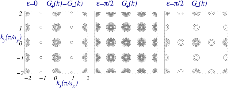
Figure 7: The expansion image for the staggered flux phase, as determined by the structure factor as a function of $(k_{x},k_{y})$. (a) For the gauge field considered ($\epsilon=0$) the two broken symmetry states have the same expansion image. (b, c) With a phase imprinting before expansion, denoted by $\epsilon$, the two states have different expansion images.

The additional freedom to imprint phases greatly enhances the information that can be extracted from expansion images. As we illustrate below, it allows important information regarding the nature of the phases to be extracted.

V.1.1 Expansion Images for Full Frustration, $\alpha=1/2$.

As explained above, the groundstate at $n_{\phi}=1/2$ is the “staggered flux” phase, which is two-fold degenerate. In the gauge (5) we have been considering, the condensate wavefunctions are given by Eq. (14), and therefore have a unit cell of size $2\times 2$. A straightforward calculation of $G^{\pm}({\bm{k}})$ shows that the two broken symmetry states have the same Fourier transform, $G^{+}({\bm{k}})=G^{-}({\bm{k}})$, illustrated in Fig. 7 (a). Therefore, the expansion image cannot discriminate between whether the groundstate is in state $\psi^{c}_{+}$ or in state $\psi^{c}_{-}$. On the other hand, the expansion image can distinguish these states from the expansion images of condensates formed from all particles condensed in either one or the other of the two single-particle states. These individual single-particle states have the full translational symmetry of the underlying system – namely under $x\to x+2a_{x}$ and $y\to y+a_{y}$ – so the Fourier components of a condensate formed from either one has peaks spaced by the reciprocal lattice vectors ${\bm{K}}_{x}=(\pi/a_{x},0)$ and ${\bm{K}}_{y}=(0,2\pi/a_{y})$. On the other hand, the “staggered flux phase” has broken translational invariance in the $y$ direction, being invariant only under the translations $y\to y+2a_{y}$, so the Fourier components are spaced by the $(\pi/a_{x},0)$ and $(0,\pi/a_{y})$. The appearance of this smaller periodicity in the $k_{y}$ direction is indicative of the broken spatial periodicity.

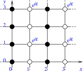
Figure 8: A pattern of phases to imprint before expansion. For $\epsilon\neq 0$, this causes the expansion images of the two staggered flux states to differ.

For the gauge used in this work, the expansion image does not distinguish between the two different staggered flux states. However, in the gauge used in Ref. Lim et al., 2008 these two states have very different expansion images. Indeed, in the gauge of Ref. Lim et al., 2008 one state has a condensate wavefunction with uniform density and phase (and therefore enjoys the full symmetry of the lattice), while the other has a phase pattern with a $2\times 2$ unit cell; these give rise to very different Fourier transforms and therefore expansion images.

As described above, the ability to locally address sites of the lattice leads to the possibility to apply a spatial phase pattern $e^{iS_{i}}$ to the system prior to expansion. This can be used to discriminate between the two staggered flux states. Specifically, we consider the case in which potentials or optical dressing is used to imprint the phase pattern

$$S_{i}=\epsilon\times{\rm mod}(x_{i},2){\rm mod}(y_{i},2)\,.$$ (27)

Thus, for the atoms on sites with $x_{i}=\mbox{odd}$ (i.e. which are all of “excited” or all “ground” states in the proposal of Ref. Gerbier and Dalibard, 2010), the phase of every other one along the $y$-direction is advanced by $\epsilon$, as illustrated in Fig. 8. This can be achieved, for example, by applying a state-selective potential with period $\Delta y=2$.

A calculation of the resulting expansion images shows that this phase pattern causes the two staggered flux phases to have different expansion images, $G_{+}({\bm{k}},\epsilon)\neq G_{-}({\bm{k}},\epsilon)$. Owing to the relation $\psi^{c}_{+}=(\psi^{c}_{-})^{*}$, it is straightforward to show that $G_{-}({\bm{k}},\epsilon)=G_{+}({\bm{k}},-\epsilon)$. The results are illustrated for $\epsilon=\pi/2$ in Fig. 7(b) and (c). There is a clear distinction between the expanstion images of the two states: e.g. the signal at $(k_{x},k_{y})=(1,1)$ is absent for $\psi_{-}$, while being strong for $\psi_{+}$. It is not, however, necessary to impose large phase difference $S_{i}$ to obtain large effects. The change in the spectrum increases linearly for non-zero $\epsilon$. As shown in Fig. 9 even very small changes of phase $\epsilon$ can give rise to notable changes in the expansion images.

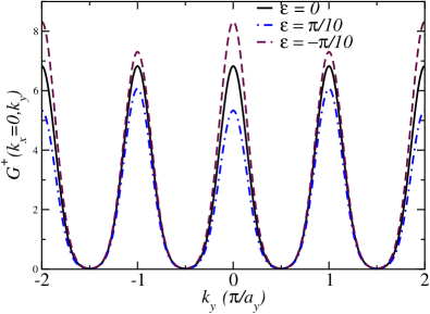
Figure 9: The expansion image of the staggered flux state is very sensitive to $\epsilon\neq 0$, here shown for $\psi^{c}_{+}$. Even a phase of $\epsilon=\pi/10$ allows for notable change. Since $G_{-}({\bm{k}},\epsilon)=G_{+}({\bm{k}},-\epsilon)$, this change allows for a discrimination between $\psi^{c}_{+}$ and $\psi^{c}_{-}$.

V.2 Measurement of the Condensate Fraction

The condensate fraction can be measured experimentally by analysing the expansion images of the lattice gas. For a perfect condensate only few a coherent peaks are visible within the Brillouin zone. Condensate depletion from strong interactions in the atomic gas results in the appearance of an additional background, i.e. some of the density of particles is spread out in the Brillouin zone. Generally, we may write the density matrix of the depleted condensate as

$$\rho_{ij}\equiv n_{c}(\psi^{c}_{i})^{*}\psi^{c}_{j}+\delta\rho_{ij},$$ (28)

where $n_{c}$ is the condensate density and $\psi^{c}_{i}$ is its wavefunction; this equation thus defines $\delta\rho_{ij}$. Similarly, the amplitudes of the expansion image can be written as

$$G({\bf{k}})\equiv n_{c}G_{c}({\bf{k}})+\Delta G({\bf{k}}),$$ (29)

where the coherent part $G_{c}(k)$ derives from the non-interacting condensate

$$G_{c}({\bf{k}})=(1/N_{s})\sum_{i,j}(\psi^{c}_{i})^{*}\psi^{c}_{j}\,e^{i{\bf{k}}({\bf{r}}_{i}-{\bf{r}}_{j})}.$$ (30)

This defines $\Delta G(k)$. Experimentally, one can only measure $G({\bf{k}})$. In order to extract $n_{c}=nx_{c}$, one needs to make some assumption about $\Delta G({\bf{k}})$. Numerically, we find that this background of the expansion image has some internal structure (and this data could be used to build a more accurate model), but to a first approximation we may assume that it is homogeneous. This translates into making the simple assumption that $\Delta G({\bf{k}})$ is independent of ${\bf{k}}$. One then obtains

$$G({\bf{k}})\equiv n_{c}G_{c}({\bf{k}})+(n-n_{c}),$$ (31)

which satisfies the proper normalisation of the Fourier amplitudes $\sum_{\bf{k}}G({\bf{k}})=\sum_{i}\rho_{ii}=N$.

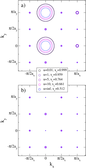
Figure 10: a) Expansion images $G({\bf{k}})$ of interacting Bose-Einstein condensates, showing the effect of condensate depletion. The data show the evolution of the condensate at $n=n_{\phi}=1/2$ on a square lattice of size $L_{x}=L_{y}=4$ for weak to hardcore interactions. The depletion of the coherent peaks is given approximately by the condensate fraction. b) The bottom panel shows the magnitude of the corrective term $\Delta G({\bf{k}})$ in Eq. (29). This data shows some structure, in particular, the background contribution is smaller at the $k$-points where coherent peaks were present then it is elsewhere.

Let us test the accuracy of this assumption for the example of a half filled lattice at $\alpha=1/2$ that was discussed in §V.1.1. To visualize the effect of condensate depletion, Fig. 10 displays the evolution of the expansion image for the case already displayed in Fig. 7(a) for a weakly interacting gas. Unlike in the single particle picture, calculations of the actual many-body wavefunction for the interacting system are limited to finite size. Data in Fig. 10 were obtained for a lattice of size $4\times 4$, so the ‘incoherent’ background occurs at peaks spaced by $\Delta k_{x}=2\pi/L_{x}=\pi/(2a_{x})$ and $\Delta k_{y}=2\pi/L_{y}=\pi/(2a_{y})$. The main features of the expansion image remain those of the pure condensate even with strong interactions, except for the partial suppression of the coherent peaks that proceeds according to (29) with $\Delta G({\bf{k}})$ given by small amplitudes. The Brillouin zone can thus be partitioned into areas with peaks $\mathcal{A}_{\text{P}}$ and the remaining background area $\mathcal{A}_{\text{BG}}$. The magnitude of this corrective term $\Delta G({\bf{k}})$ is shown in Fig. 7(b). Its spatial dependency is weak, excepting the notably smaller correction within $\mathcal{A}_{\text{P}}$ as compared to the overall background $\mathcal{A}_{\text{BG}}$. Therefore, the average amplitude in the background

$$n-n_{c}\simeq\langle I(\mathcal{A}_{\text{BG}})\rangle=\mathcal{A}_{\text{BG}}^{-1}\sum_{{\bf{k}}\in\mathcal{A}_{\text{BG}}}G({\bf{k}})$$ (32)

is a proxy for the level of condensate depletion $(n-n_{c})$. Applied to the case with hardcore interactions in Fig. 10, we deduce a condensate fraction of $n_{c}=0.214$ from the intensity of the background, which should be compared to the exact value of $n_{c}=0.256$. This estimate is rather crude, as the background also contributes some signal within $\mathcal{A}_{\text{P}}$. A more accurate value is obtained allowing for such a contribution $\langle\delta I(\mathcal{A}_{\text{P}})\rangle\equiv\kappa\langle I(\mathcal{A}_{\text{BG}})\rangle$, where $\kappa$ is a ‘coherence’ factor for the addition between the coherent condensate wavefunction and the incoherent background. The corrected estimate becomes

$$n-n_{c}=\frac{\mathcal{A}_{\text{BG}}+\kappa\mathcal{A}_{\text{P}}}{\mathcal{A}_{\text{BG}}+\mathcal{A}_{\text{P}}}\langle I(\mathcal{A}_{\text{BG}})\rangle,$$ (33)

which reduces to (32) in the limit of sharp coherence peaks $\mathcal{A}_{\text{P}}\to 0$. For the data in Fig. 10, we find exact values of $\kappa$ in the range of 0.4 to 0.5. Assuming $\kappa=0.45$, the exact condensate depletion is reproduced to within 1% accuracy.

VI Summary

We have studied the groundstates of two-dimensional frustrated Bose-Hubbard models. We have focused on the situation in which the imposed gauge fields give rise to a pattern of staggered fluxes, of magnitude $\alpha$ and of alternating sign along one of the principal axes. For $\alpha=1/2$ this model is equivalent to the case of uniform flux $n_{\phi}=1/2$, which is the “fully frustrated” XY model with time-reversal symmetry. We have shown that, for $\alpha_{c}<\alpha<1/2$, with $\alpha_{c}\approx 0.389$, the mean-field groundstate breaks translational invariance, giving rise to a density wave pattern. For $\alpha=1/2$ the mean-field groundstate breaks both translational symmetry and time-reversal symmetry, forming the staggered flux phase which has uniform density but circulating gauge-invariant currents.

We have introduced a general numerical technique to detect broken symmetry condensates in exact diagonalization studies. Using this technique we have shown that, for all cases studied, the Bose-Hubbard model with staggered flux $\alpha$ is condensed. We have obtained quantitative determinations of the condensate fractions. In particular, our results establish that the fully frustrated quantum XY model is condensed at zero temperature, with a condensate fraction of $x_{c}\simeq 0.4$.

The low-temperature condensed phases that appear in this system are of significant interest in connection with their thermal phase transitions into the high-temperature normal phase. The groundstate of the fully frustrated system breaks both $U(1)$ and $Z_{2}$ symmetries (owing to both Bose-Einstein condensation, and the combination of translational symmetry breaking and time-reversal symmetry breaking). The transition to the high-temperature phase is interesting, combining the physics of the Kosterlitz-Thouless transition [$U(1)$] with an Ising transition ($Z_{2}$), and its properties have stimulated much theoretical debate.Martinoli and Leemann (2000); Fazio and van der Zant (2001) The cold atom system described here will allow this transition to be studied also in a highly quantum regime, with of order one particle per lattice site, that is inaccessible in frustrated Josephson junction arrays.Polini et al. (2005) Our results show that the staggered flux model leads also to other cases that break $U(1)$ and $Z_{3}$ (or higher $Z_{p}$ symmetry depending on the flux $\alpha$). There is also the possibility to study commensurate/incommensurate transitions driven by locking of the density wave order to the underlying lattice.

We discussed in detail the experimental consequences of our results. In our discussion, we have explained the meaning of gauge-invariance in ultracold atom systems subject to optically induced gauge potentials: Expansion images are gauge-dependent, and (provided gauge fields are absent during expansion) measure the canonical momentum distribution. Furthermore, we have shown how the ability to imprint phase patterns prior to expansion (analogous to an instantaneous change of gauge) can allow very useful additional information to be extracted from expansion images.