FTPI-MINN-10/24, UMN-TH-2916/10

Perturbative Aspects of Heterotically Deformed
CP$(N-1)$ Sigma Model. I

Xiaoyi Cui${}^{\,a}$ and M. Shifman${}^{\,b}$

^aPhysics Department, University of Minnesota, Minneapolis, MN 55455, USA
^bWilliam I. Fine Theoretical Physics Institute, University of Minnesota, Minneapolis, MN 55455, USA 
and
Jefferson Physical Laboratory, Harvard University, Cambridge, MA 02138, USA

Abstract

In this paper we begin the study of renormalizations in the heterotically deformed $\mathcal{N}=(0,2)$ CP$(N-1)$ sigma models. In addition to the coupling constant $g^{2}$ of the undeformed $\mathcal{N}=(2,2)$ model, there is the second coupling constant $\gamma$ describing the strength of the heterotic deformation. We calculate both $\beta$ functions, $\beta_{g}$ and $\beta_{\gamma}$ at one loop determining the flow of $g^{2}$ and $\gamma$. Under a certain choice of the initial conditions, the theory is asymptotically free. The $\beta$ function for the ratio $\rho=\gamma^{2}/g^{2}$ exhibits an infrared fixed point at $\rho=1/2$. Formally this fixed point lies outside the validity of the one-loop approximation. We argue, however, that the fixed point at $\rho=1/2$ may survive to all orders. The reason is the enhancement of symmetry – emergence of a chiral fermion flavor symmetry in the heterotically deformed Lagrangian – at $\rho=1/2$. Next we argue that $\beta_{\rho}$ formally obtained at one loop, is exact to all orders in the large-$N$ (planar) approximation. Thus, the fixed point at $\rho=1/2$ is definitely the feature of the model in the large-$N$ limit.

1 Introduction

Two-dimensional CP$(N-1)$ models emerged as effective low-energy theories on the worldsheet of non-Abelian strings in a class of four-dimensional ${\mathcal{N}}=2\,$  gauge theories [1, 2, 3, 4] (for reviews see [5]). Deforming these models in various ways (i.e. breaking supersymmetry down to ${\mathcal{N}}=1$) one arrives at heterotically deformed CP$(N-1)\,$models [6, 7, 8, 9] (heterotic CP$(N-1)\,$models for short), a very interesting and largely unexplored class of models characterized by two coupling constants: the original asymptotically free coupling and an extra one describing the strength of the heterotic deformation. These two-dimensional models are of importance on their own, since they exhibit highly nontrivial dynamics, with a number of phase transitions. This fact was recently revealed [10] in the large-$N$ solution of the model (see also [11]).

Our current task is to analyze perturbative aspects of the heterotic CP$(N-1)\,$ models. General aspects of perturbation theory in the $\mathcal{N}=(0,2)$ models were discussed by Witten [12]. We will study particular renormalization properties and calculate the $\beta$ functions in the CP$(N-1)$ models heterotically deformed in a special way. In this first paper of a series we will focus on one-loop effects and demonstrate that both couplings of the model enjoy asymptotic freedom (AF). Moreover, we observe a special fixed-point regime in the infrared (IR) domain and argue that it holds beyond one loop.

Written in components, the Lagrangian of the heterotic CP(1) model takes the form [7]

$${\mathcal{L}}_{(2,2)}=G\left\{\partial^{\mu}\phi\partial_{\mu}\phi^{\dagger}+i\bar{\psi}\not{\partial}\psi-{2i}\,\frac{1}{\chi}\,\bar{\psi}\gamma^{\mu}\psi\,\phi^{\dagger}\partial_{\mu}\phi-\frac{2}{\chi^{2}}\,\psi_{L}^{\dagger}\psi_{L}\,\psi_{R}^{\dagger}\psi_{R}\right\}\,,$$ (1)

and 

$${\mathcal{L}}_{(0,2)}=\zeta_{R}^{\dagger}\,i\partial_{L}\,\zeta_{R}+\left[\frac{\gamma}{g^{2}}\,\zeta_{R}\,R\,\big{(}i\,\partial_{L}\phi^{\dagger}\big{)}\psi_{R}+{\rm H.c.}\right]$$

$$+\frac{|\gamma|^{2}}{g^{2}}\left(\zeta_{R}^{\dagger}\,\zeta_{R}\right)\left(R\,\psi_{L}^{\dagger}\psi_{L}\right)+G\,\left\{\frac{2|\gamma|^{2}}{g^{2}\chi^{2}}\,\psi_{L}^{\dagger}\,\psi_{L}\,\psi_{R}^{\dagger}\,\psi_{R}\right\}\,,$$ (2)

where $G$ is the Kähler metric on the target space,

$$G=\frac{2}{g^{2}\,\chi^{2}}\,,$$ (3)

$R$ is the Ricci tensor,

$$R=\frac{2}{\chi^{2}}\,,$$ (4)

and we use the notation

$$\chi\equiv 1+\phi\,\phi^{\dagger}\,.$$ (5)

The coupling $g^{2}$ enters through the metric, while the deformation coupling $\gamma$ appears in Eq. (2). Both couplings can be chosen to be real. Setting $g^{2}$ to be real means we will not consider the topological term $\varepsilon_{\mu\nu}\partial^{\mu}\phi\partial^{\nu}\phi^{\dagger}$ in this paper. To make $\gamma$ real, one should perform a phase rotation of the bosonic field $\phi$ absorbing the phase of $\gamma$ (see the first line in Eq. (2)). In fact, this corresponds to a kind of $R$-symmetry, as the reader will see from the $\mathcal{N}=(0,2)$ superfield formalism In Sec. 2. Our main results are presented by the following expressions for the one-loop $\beta$ functions:

$$\beta_{g} \equiv \frac{\partial}{\partial\text{ln}\mu}g^{2}(\mu)=-\frac{g^{4}}{2\pi}+...$$ (6)

$$\beta_{\gamma} \equiv \frac{\partial}{\partial\text{ln}\mu}\gamma(\mu)=\frac{\gamma}{2\pi}\left(\gamma^{2}-g^{2}\right)+...$$ (7)

where ellipses stand for two-loop and higher-order terms. The heterotic deformation does not affect $\beta_{g}$ which stays the same as in the ${\mathcal{N}}=(2,2)$ CP(1) model. Among other results, we calculate the law of running of the ratio

$$\rho=\frac{\gamma^{2}}{g^{2}}\,$$

see Eq. (50). If at any renormalization point, in particular, in the ultraviolet (UV) limit, $\rho$ is chosen to be smaller than $1/2$, in the IR limit it runs to $\rho\to 1/2$, which is the fixed point for this parameter. With $\rho\leq 1/2$, the theory is asymptotically free. Analogs of Eqs. (6) and (7) in the heterotic CP$(N-1)$ model with arbitrary $N$ are presented in (55) and (57).

The paper is organized as follows. In Sec. 2, we describe the model using both superfield language and component field language. We show that the $\mathcal{N}=(0,2)$ deformation structure is quite unique in certain sense. In Sec. 3, we show that by symmetry analysis, the renormalization structure of the deformation term is constrained. Conceptually it gives partially the answer for why the deformation term does not get renormalized at one-loop level. In Sec. 4 we describe the linear background field method and calculate the one-loop $\beta$ function for $g^{2}$ as an example. This will be useful in the two-loop calculations shown in our subsequent paper. In Sec. 5 we calculate the Z-factor wave-function renormalizations for the field $\zeta_{R}$ and $\psi_{R}$. In Sec. 6 we calculate the one-loop $\beta$ function for $\gamma$, and thus verify our expectation in Sec. 3. In Sec. 7 we discuss the running of the two couplings. We find the region that is good for perturbative calculation, and we find an IR fixed point of $\rho$ that exists universally at one-loop order. In Sec. 8 we generalize the result to CP$(N-1)$ model. We show that a factorization of $\beta_{\rho}$ survives in all loop orders. In the subsequent paper we will discuss the result from the two-loop calculation.

2 $\mathcal{N}=(0,2)$ CP(1) sigma model

Here we will briefly review basics of the heterotic CP(1) model. The metric (3) is the Fubini–Study metric of the two-dimensional sphere $S^{2}$. It is not difficult to see that the Lagrangian ${\mathcal{L}}_{(2,2)}+{\mathcal{L}}_{(0,2)}$ is invariant with respect to the joint U(1) rotations of the fields $\phi$ and $\psi$, and, in addition, invariant under the following nonlinear transformations:

$$\phi\rightarrow\phi+\alpha+\alpha^{\dagger}\phi^{2}\,,\qquad\phi^{\dagger}\rightarrow\phi^{\dagger}+\alpha^{\dagger}+\alpha\phi^{\dagger 2},$$

$$\psi\rightarrow\psi+2\alpha^{\dagger}\phi\psi\,,\qquad\bar{\psi}\rightarrow\bar{\psi}+2\alpha\phi^{\dagger}\bar{\psi}.$$ (8)

Here $\alpha$ is a complex constant. The above transformations tell us that $\phi$ transforms as the coordinate of the target manifold (a 2-sphere), and the fields $\psi$ and $\partial^{\mu}\phi$ transform as the tangent vectors.

Supersymmetry of this model is best understood via its superfield description. The $\mathcal{N}=(0,2)$ model description can be obtained by either integrating out the Grassmannian variables $\theta_{L}$ and $\theta_{L}^{\dagger}$ [7], or by constructing the model from $\mathcal{N}=(0,2)$ superfields. We will follow the second way, for reasons which will become clear shortly. We define the left and right derivatives as follows.

$$\partial_{L}=\partial_{t}+\partial_{z}\,,\qquad\partial_{R}=\partial_{t}-\partial_{z}\,.$$ (9)

The shifted space-time coordinates that satisfy the chiral condition are defined as

$$x^{0}_{L}=t+i\theta_{R}^{\dagger}\theta_{R}\,,\qquad x^{1}_{L}=z+i\theta_{R}^{\dagger}\theta_{R}\,.$$ (10)

We start from two chiral $\mathcal{N}=(0,2)$ superfields $A$ and $B$,

$$A(x^{\mu}_{L},\theta_{R})=\phi(x^{\mu}_{L})+\sqrt{2}\theta_{R}\psi_{L}(x^{\mu}_{L})\,,$$

$$B(x^{\mu}_{L},\theta_{R})=\psi_{R}(x^{\mu}_{L})+\sqrt{2}\theta_{R}F(x^{\mu}_{L})\,.$$ (11)

The supersymmetry transformations are

$$\delta_{R}\phi=\sqrt{2}\epsilon_{R}\psi_{L}\,,\qquad\delta_{R}\psi_{L}=-\sqrt{2}i\epsilon_{R}^{\dagger}\partial_{L}\phi\,,$$

$$\delta_{R}\psi_{R}=\sqrt{2}\epsilon_{R}F\,,\qquad\delta_{R}F=-\sqrt{2}i\epsilon_{R}^{\dagger}\partial_{L}\psi_{R}\,.$$ (12)

In terms of these ${\mathcal{N}}=(0,2)\,$superfields, it is not difficult to show that the Lagrangian

$$\mathcal{L}_{(2,2)}=\frac{2}{g^{2}}\,\int d^{2}\theta_{R}\left\{\frac{iA^{\dagger}\partial_{R}A-iA\partial_{R}A^{\dagger}}{1+A^{\dagger}A}+\frac{2B^{\dagger}B}{(1+A^{\dagger}A)^{2}}\right\}\rule{0.0pt}{25.60747pt}$$ (13)

identically reproduces Eq. (1).

Needless to say, this Lagrangian is $\mathcal{N}=(0,2)$ invariant, by construction. Next, we must show that it is target-space invariant. The global U(1) symmetry of Eq. (13) is obvious. As far as the nonlinear transformations Eq. (8) are concerned, for the first term we have

$$\delta_{\alpha}\,\frac{A\partial_{R}A^{\dagger}+A^{\dagger}\partial_{R}A}{1+A^{\dagger}A}\propto\left(\alpha\partial_{R}A^{\dagger}+\alpha^{\dagger}\partial_{R}A\right),\rule{0.0pt}{25.60747pt}$$ (14)

which is a combination of holomorphic and antiholomorphic functions, and thus should vanish in the action. Moreover, one can show that the second term is invariant by itself, i.e.,

$$\delta_{\alpha}\,\frac{B^{\dagger}B}{(1+A^{\dagger}A)^{2}}=0\,.$$ (15)

The relative coefficient between the first and the second terms in Eq. (13) is unity because of the $\mathcal{N}=(2,2)$ symmetry which is implicit in Eq. (13). One can, of course, introduce another coupling constant in front of the term quadratic in the $B$ field, but then one can always absorb such constant in the normalization of $B$.

Thus, with the given set of fields, starting from ${\mathcal{N}}=(0,2)\,$supersymmetry, we get an enhanced $\mathcal{N}=(2,2)$ supersymmetry “for free.” This phenomenon is similar to the $\mathcal{N}=(1,1)$ case, as shown in [13] (see also [14]).

This gives us a hint on the way of converting the $\mathcal{N}=(2,2)$ model into its heterotic $\mathcal{N}=(0,2)$ extension. Namely, one should add an interaction of the field $B$ with $A$ and $A^{\dagger}$ without involving the field $B^{\dagger}$. Taking into consideration the target space symmetry, one can come up with the following deformation Lagrangian:

$$\Delta\mathcal{L}=-\int d^{2}\theta_{R}\,\frac{4\gamma}{g^{2}}\,\frac{BA^{\dagger}}{1+A^{\dagger}A}+{\rm H.c.}\,.$$ (16)

The coupling $\gamma$ has dimension $m^{1/2}$, and must be viewed as a complex Grassmann number. Now, in components, the deformation Lagrangian takes the form

$$\Delta\mathcal{L}=\left[\gamma\,G(i\partial_{L}\phi^{\dagger})\psi_{R}+{\rm H.c.}\right]+|\gamma|^{2}(G\psi_{R}^{\dagger}\psi_{R})\,.$$ (17)

The above construction, however, suffers from the fermion number nonconservation. The very last step which fixes this problem is promoting $\gamma$ to a dynamic superfield. To this end we introduce a chiral superfield 

$$\mathcal{B}=\zeta_{R}+\sqrt{2}\theta_{R}\mathcal{F}\,,$$ (18)

and then replace $\gamma$ by

$$\gamma\to\gamma\,\mathcal{B}\,.$$ (19)

As a result, the deformation Lagrangian takes the form

$$\Delta\mathcal{L} = \int d^{2}\theta_{R}\left\{\left[-\frac{4\gamma}{g^{2}}\,\frac{\mathcal{B}BA^{\dagger}}{1+A^{\dagger}A}+{\rm H.c.}\right]+2\mathcal{B}^{\dagger}\mathcal{B}\right\}$$ (20)

$$= i\zeta_{R}^{\dagger}\partial_{L}\zeta_{R}+\left[\gamma\,\zeta_{R}\,G(i\partial_{L}\phi^{\dagger})\psi_{R}+{\rm H.c.}\right]$$

$$+|\gamma|^{2}(\zeta_{R}^{\dagger}\zeta_{R})(G\psi_{R}^{\dagger}\psi_{R})+|\gamma|^{2}G^{2}\psi_{L}^{\dagger}\psi_{L}\psi_{R}^{\dagger}\psi_{R}\,.$$

The target space invariance can be verified at the level of superfields,

$$\delta_{\alpha}\,\frac{\mathcal{B}BA^{\dagger}}{1+A^{\dagger}A}\propto\alpha^{\dagger}\mathcal{B}B\,,$$ (21)

which vanishes in the action. Needless to say, the $S^{2}$ target space transformations of ${\mathcal{B}}$ are trivial, $\delta{\mathcal{B}}=0$.

Finally, we comment on the absorption of the U$(1)$ phase of the coupling $\gamma$ in this context. This means that whenever $\gamma=|\gamma|e^{i\omega}$, we can always redefine $\gamma\to\gamma e^{-i\omega}$ and $A^{\dagger}\to A^{\dagger}e^{i\omega}$ supplemented by a $\theta_{R}$ rotation. So $\gamma$ can always be kept real. Notably, this rotation only involves bosons. This is because, we can assign a proper U$(1)$ charge to $\theta_{R}$ to keep $\psi_{L}$ U$(1)$-neutral. Thus the rotation actually corresponds to a kind of $R$-symmetry. It is anomaly-free.

3 Global symmetries and renormalization structure

In this section we analyze the renormalization structure of the heterotic CP(1) model. In the deformed model we have two dimensionless couplings, $g$ and $\gamma$. The first one is related to geometry of the target space, and the second one parametrizes the strength of the heterotic deformation. The first question to ask at one-loop level is that whether or not there is mixing between these two couplings. In addition, we should verify that other structures, which are absent in Eq. (13) and Eq. (20), do not show up as a result of loop corrections. What can be said from analyzing the symmetries of the model at hand? We will follow the line of reasoning similar to the proof [15] of nonrenormalization theorems for superpotentials in four dimensions. We start from the U(1) symmetries. There are three generalized U(1) symmetries listed in Table 1, with the corresponding charge assignments.

Fields	U$(1)_{1}$	U$(1)_{2}$	U$(1)_{3}$
$\gamma$	$1$	$0$	$-\frac{1}{2}$
$A$	$0$	$1$	$-\frac{1}{2}$
$B$	$0$	$1$	$\frac{1}{2}$
$\mathcal{B}$	$-1$	$0$	$-\frac{1}{2}$

Table 1: Generalized U(1) symmetries of the heterotically deformed CP(1) model.

Using these charge assignments one can show that the only nontrivial combination of $\gamma$, $A^{\dagger}$, $B$, and $\mathcal{B}$ invariant under all U(1) symmetries is given by $\gamma\mathcal{B}BA^{\dagger}$.

Since $\Delta{\mathcal{L}}$ presents the integral over $d\theta_{R}$ and $d\theta_{R}^{\dagger}$, (unfortunately), it is not analogous to $F$ terms in conventional supersymmetric Lagrangians. Hence, with radiative corrections included, $\Delta{\mathcal{L}}$ can possibly contain U(1)-neutral pairs such as $A^{\dagger}A$, $B^{\dagger}B$, $\mathcal{B}^{\dagger}\mathcal{B}$ and the modulus of the coupling $|\gamma|^{2}$. Due to dimensional reasons, $B^{\dagger}B$ could only show up in the combination of the type ${B^{\dagger}B}/{\mathcal{B}^{\dagger}\mathcal{B}}$, which, obviously, cannot happen in loops provided our theory is properly regularized in the infrared domain (and, of course, it will be regularized both in the IR and UV domains). Its absence can also be verified by analyzing a fermionic SU$(2)$ symmetry discussed in Sec. 5.

As for $A^{\dagger}A$, this term is constrained by the non-linear target space symmetry. The only allowed form is the combination

$$\frac{BA^{\dagger}}{1+A^{\dagger}A}$$

and its Hermitian conjugate. This shows that the structure of the deformation is quite unique. Corrections in $g^{2}$ are strongly constrained too, as we will see momentarily. Thus, the corrections that can show up in loops are $O(\gamma^{2})$, $O(\gamma^{2}g^{2})$, $O(\gamma^{4})$, and so on.

The latter circumstance becomes clear if we take into consideration that the operator $R\partial_{L}\phi^{\dagger}\psi_{R}$ is, in fact, the superconformal anomaly of the undeformed theory [7],

$$J_{sc,L}=\frac{-i\sqrt{2}}{2\pi}\frac{\partial_{L}\phi^{\dagger}\psi_{R}}{\chi^{2}}\,.$$ (22)

Since the supercurrent is conserved, $R\partial_{L}\phi^{\dagger}\psi_{R}$ receives no corrections in $g^{2},\,\,g^{4},$ etc. Certainly, on general grounds we can not exclude corrections of the type $|\gamma|^{2}g^{2}$, but these can show up only in the second and higher loops. Therefore, at one loop the corrections to $\gamma$ come from $O(|\gamma|^{2})$ one-particle irreducible correction to the vertex, and the $Z$ factors of the fields of which the deformation term is built. Calculation of the $Z$ factors is carried out in Sect. 5. We check all assertions made above on general grounds by explicit calculation of relevant diagrams in Sect. 6.

4 Background field method. One-loop $\beta$ function for $g^{2}$

We will see shortly that $\beta_{g}$ is unaffected by the heterotic deformation at one loop. Before passing to direct calculations of the $Z$-factors for the fields $\zeta_{R}$, $\psi_{R}$, let us outline generalities of the background field method [16]. The full power and efficiency of this method will become clear in two-loop calculations [17]. Here will just “calibrate” it in the simple problem of the one-loop $\beta$ function $\beta_{g}$. The result is well-known, of course [18]; therefore, this exercise [16] is needed mostly to introduce necessary conventions and notations.

Each field is decomposed into a background part (large part) and a quantum part (small fluctuations to be integrated over). One can simplify calculations by making a particularly convenient choice of the background fields, which may vary from problem to problem. Then one expands the Lagrangian in the given background, in terms of quantum fields. Linear terms can be omitted. Quadratic terms determine one-loop corrections. Cubic and higher order terms are needed for two-loop calculations, i.e. for higher orders. The two-loop calculations will be presented in a forthcoming paper [17]. Note that, generally speaking, the background field does not have to respect the symmetry of the theory. However, the full symmetry must certainly be present in the final answer for ${\mathcal{L}}_{\rm eff}$.

After this remark we proceed to an instructive one-loop calculation of $\beta_{g}$. The split of the fields is

$$\phi\to\phi_{0}+q$$ (23)

where $q$ represents the quantum part to be integrated over in loops. For the background part we choose in the problem at hand

$$\phi_{0}=fe^{-ikx}\,,\qquad\phi_{0}^{\dagger}=f^{\dagger}e^{ikx}\,,\qquad\phi_{0}^{\dagger}\phi_{0}=f^{\dagger}f\,,$$ (24)

where $f$ is a constant, and at the very end (after separating all terms quadratic in $k$) we can tend $k\to 0$. The fermion field is quantum, by definition. The background field expression for the Lagrangian is

$$\mathcal{L}_{0}=\frac{2}{g_{0}^{2}}\,\frac{k^{2}\,f^{\dagger}f}{(1+f^{\dagger}f)^{2}}\,,$$ (25)

where $g_{0}$ is the bare coupling (i.e. the coupling constant at the UV cut-off $M_{\rm uv}$. We will concentrate on the boson contribution because the fermion loop at this level is finite and, thus, does not contribute to the $\beta$ function, see Appendix B. The results in this appendix will be used in two-loop calculations.

Expanding the Lagrangian up to the second order in the quantum fields, we obtain

$$\mathcal{L}_{\phi(1)} = (G^{1,0}_{0}q+G^{0,1}_{0}q^{\dagger})\partial_{\mu}\phi_{0}\partial^{\mu}\phi^{\dagger}_{0}+G_{0}(\partial_{\mu}q\partial^{\mu}\phi^{\dagger}_{0}+\partial_{\mu}\phi_{0}\partial^{\mu}q^{\dagger})\,,$$

$$\mathcal{L}_{\phi(2)} = (G^{2,0}_{0}q^{2}+G^{0,2}_{0}q^{\dagger 2}+G^{1,1}_{0}qq^{\dagger})\partial_{\mu}\phi_{0}\partial^{\mu}\phi^{\dagger}_{0}$$ (26)

$$+ (G^{1,0}_{0}q+G^{0,1}_{0}q^{\dagger})(\partial_{\mu}q\partial^{\mu}\phi^{\dagger}_{0}+\partial_{\mu}\phi_{0}\partial^{\mu}q^{\dagger})+G_{0}\partial_{\mu}q\partial^{\mu}q^{\dagger}$$

where

$$\left.G^{i,j}_{0}\equiv\frac{1}{i!j!}\,\frac{\partial^{i}}{\partial\phi^{i}}\frac{\partial^{j}}{\partial\phi^{j\dagger}}\frac{2}{g^{2}_{0}\,(1+\phi\phi^{\dagger})^{2}}\right|_{\phi_{0},\phi^{\dagger}_{0}}\,,$$ (27)

and the metric $G_{0}$ coincides with the quantity $G_{0}^{0,0}$ defined in Eq. (27). In what follows we may drop the subscript $0$ on some quantities, whose meaning is obvious from the context. In the first line in Eq. (26) extra source terms (irrelevant for what follows) may be necessary in order to discard $\mathcal{L}_{\phi(1)}$ because of its proportionality to the equation of motion for the given background field.

In calculating the graphs which determine the $\beta$ function one should keep in mind that they are divergent both in the ultraviolet and infrared. To regularize the UV divergence we will use dimensional reduction working in $D=2-\epsilon$ dimensions. To regularize the IR divergence we introduce a small mass term for the quantum field (see [16]),

$${\mathcal{L}}_{m}=G_{0}\left(-m_{0}^{2}q^{\dagger}q-m_{0}\bar{\psi}\psi\ \right)\,.$$ (28)

At the very end both regularizing parameters, $m_{0}$ and $\epsilon$ are supposed to tend to zero. In logarithmically divergent graphs the following correspondence takes place at one loop:

$$\frac{1}{\epsilon}\,\leftrightarrow\,\text{ln}\frac{M_{\rm uv}}{m_{0}}\,,$$ (29)

where the left-hand side represents dimensional regularization, while the right-hand side the Pauli–Villars regularization; $M_{\rm uv}$ is the mass of the Pauli–Villars regulator.

Now we can pass to one-loop calculation. The relevant boson diagrams are depicted in Fig. 1. (Fermion-loop diagrams do not contribute to $\beta$ functions at the one loop level in both, the undeformed and deformed models. We discuss them at the end of this section.)

Figure 1: Boson loops contributing to the one-loop $\beta$ function. The wavy lines stand for the background field $\partial_{\mu}\phi_{0}$ while the dashed lines for $q$.

For dimensional reasons we need each diagram to be at most quadratic in $\partial^{\mu}\phi_{0}$. Higher orders in this parameter will not contribute to the effective action (see Eq. (25)). As a result we arrive at the following contributions to the effective Lagrangian:

$$(a) = iG^{1,1}\partial^{\mu}\phi_{0}\partial_{\mu}\phi_{0}IG^{-1}\,,$$ (30)

$$(b) = \frac{i}{2d}\{{G^{1,0}}^{2}\partial_{\mu}\phi\partial^{\mu}\phi_{0}+{G^{0,1}}^{2}\partial_{\mu}\phi^{\dagger}_{0}\partial^{\mu}\phi^{\dagger}_{0}\}IG^{-2}$$ (31)

$$-\frac{i}{2}G^{1,0}G^{0,1}\left(\partial_{\mu}\phi_{0}\partial^{\mu}\phi^{\dagger}_{0}\right)I\,G^{-2}\,,$$

where we define the integral ($d=2-\epsilon$)

$$I=\int\frac{d^{d}p}{(2\pi)^{d}}\,\frac{1}{p^{2}-m^{2}}=-\frac{i}{4\pi}\Gamma\left(\frac{\epsilon}{2}\right)\,\left(\frac{\sqrt{4\pi}}{m}\right)^{\epsilon}=-\frac{i}{2\pi\epsilon}+O(\epsilon^{0})\,.$$ (32)

We will have many encounters with this universal integral later.

Using $\phi_{0}$ from Eq. (24) and assembling Eq. (30) – (31) we arrive at the following effective one-loop Lagrangian:

$$\Delta{\mathcal{L}}_{1} = ik^{2}\,I\,\left[G^{1,1}Gf^{\dagger}f-\frac{1}{4}\left({G^{1,0}}\right)^{2}f^{2}-\frac{1}{4}\left({G^{0,1}}\right)^{2}f^{\dagger 2}-\frac{1}{2}G^{1,0}G^{0,1}f^{\dagger}f\right]G^{-2}$$ (33)

$$= -2ik^{2}f^{\dagger}fI\frac{1}{(1+f^{\dagger}f)^{2}}\,,$$

to be compared with Eq. (25). This one-loop result obviously maintains the target-space symmetries. The integral $I$ can be readily calculated upon transition to the Euclidean space,

$$I=\frac{-i}{(4\pi)^{d/2}}\Gamma\left(1-\frac{d}{2}\right)\left(m^{2}\right)^{-1+\frac{d}{2}}\,,$$ (34)

cf. Eq. (32). Finally, we arrive at

$$\Delta{\mathcal{L}}_{1}=-\frac{2}{(1+\phi^{\dagger}\phi)^{2}}\partial^{\mu}\phi^{\dagger}\partial_{\mu}\phi\cdot\frac{1}{4\pi m^{\epsilon}}\,\frac{2}{\epsilon}\,.$$ (35)

Comparing with Eq. (25) it is easy to see that

$$\frac{1}{g^{2}}=\frac{1}{g^{2}_{0}}-i\,I=\frac{1}{g^{2}_{0}}-\frac{1}{2\pi}\,\text{ln}\frac{M_{\rm uv}}{m}\,.$$ (36)

Now, the general definition of the $\beta$ function

$$\beta_{g}=\left(\partial/\partial{\rm ln}(m)\right)g^{2}(m)$$ (37)

implies the following one-loop $\beta$ function:

$$\beta_{g}=-\frac{g^{4}}{2\pi}\,.$$ (38)

We end this section by commenting on the fermion diagrams. In the undeformed $\mathcal{N}=(2,2)$ model, the relevant diagram is the $T$ product of two fermion U$(1)$ currents $\bar{\psi}\gamma^{\mu}\psi$ (Fig. 6), which is finite due to transversality. Moreover, this remains to be the case in the deformed $\mathcal{N}=(0,2)$ model too — all relevant fermion diagrams have no $\ln M_{\rm uv}/\mu$. A more detailed argumentation can be found in Appendix B. Thus, Eq. (38) presents the full contribution at one loop.

5 $Z$-factors

The renormalization of the term $\mathcal{B}BA^{\dagger}(1+A^{\dagger}A)^{-1}$ is determined by one-particle irreducible corrections to the vertex and the wave-function renormalization for $\psi_{R}$ and $\zeta_{R}$. Here we will deal with the corresponding $Z$ factors, $Z_{\zeta}$ and $Z_{\psi_{R}}$ (for brevity the latter will be denoted as $Z_{\psi}$).

A closer look at the Lagrangian given in Eqs. (13) and (20), tells us that this Lagrangian is invariant under a SU$(2)$ rotation of $\mathcal{B}$ and $\frac{B}{1+A^{\dagger}A}$. If we define a SU$(2)$ superfield doublet

$$\Psi=\left(\begin{smallmatrix}\frac{\sqrt{2}B}{g(1+A^{\dagger}A)}\\ \mathcal{B}\end{smallmatrix}\right)\,,$$ (39)

the part that involves all right-handed fermions (i.e., all but the first terms in Eq. (41)) can be rewritten as

$$2\Psi^{\dagger}_{a}\Psi_{a}+\sqrt{2}\left[\frac{\gamma}{g}A^{\dagger}\varepsilon^{ab}\Psi_{a}\Psi_{b}+{\rm H.c.}\right]\,,$$ (40)

which is obviously SU$(2)$ invariant. This symmetry has a discrete symmetry inside, which is not affected by fermion anomalies. So we conclude that the wave-function renormalization for $\psi_{R}\,\sqrt{\frac{2}{g^{2}\chi^{2}}}$ on the one hand, and for $\zeta_{R}$ on the other, must be the same,

$$Z_{\zeta}=Z_{\psi}\,.$$

In addition to the perturbative calculation presented below, this can also be indirectly deduced from Chen’s analysis [19] of the fermion zero modes in the instanton background.

Now we are ready to carry out the actual calculation to verify the above expectation, and calculate the wave-function renormalizations for $\psi_{R}$ and $\zeta_{R}$. We start from the Lagrangian with the bare couplings in UV,

$$\mathcal{L}_{0} = \int d^{2}\theta_{R}\frac{2}{g_{0}^{2}}\left\{\frac{A\partial_{R}A^{\dagger}+A^{\dagger}\partial_{R}A}{1+A^{\dagger}A}+\frac{2B^{\dagger}B}{(1+A^{\dagger}A)^{2}}\right\}+2\mathcal{B}^{\dagger}\mathcal{B}$$ (41)

$$-\frac{4}{g_{0}^{2}}\left[\frac{\gamma_{0}\,\mathcal{B}BA^{\dagger}}{1+A^{\dagger}A}+{\rm H.c.}\right]\,,$$

and evolve it down, where we have

$$\mathcal{L}_{\text{eff}} = \int d^{2}\theta_{R}\frac{2}{g^{2}}\left\{\frac{A\partial_{R}A^{\dagger}+A^{\dagger}\partial_{R}A}{1+A^{\dagger}A}+Z_{\psi}\frac{2B^{\dagger}B}{(1+A^{\dagger}A)^{2}}\right\}+2Z_{\zeta}\mathcal{B}^{\dagger}\mathcal{B}$$ (42)

$$-\frac{4}{g_{0}^{2}}Z_{\gamma}\left[\frac{\gamma_{0}\,\mathcal{B}BA^{\dagger}}{1+A^{\dagger}A}+{\rm H.c.}\right]\,.$$

Finally, we redefine the fields $\mathcal{B}$ and $B$ to absorb the $Z_{\zeta}$ and $Z_{\psi}$ factors. With this absorption done, we get

$$\mathcal{L}_{\text{eff}} = \int d^{2}\theta_{R}\frac{2}{g^{2}}\left\{\frac{A\partial_{R}A^{\dagger}+A^{\dagger}\partial_{R}A}{1+A^{\dagger}A}+\frac{2B^{\dagger}B}{(1+A^{\dagger}A)^{2}}\right\}+2\mathcal{B}^{\dagger}\mathcal{B}$$ (43)

$$-\frac{4}{g_{0}^{2}}\frac{Z_{\gamma}}{\sqrt{Z_{\psi}Z_{\zeta}}}\left[\frac{\gamma_{0}\,\mathcal{B}BA^{\dagger}}{1+A^{\dagger}A}+{\rm H.c.}\right]\,.$$

The one-particle irreducible diagrams for $Z_{\zeta}$ and $Z_{\psi}$ are shown in Fig. 2. The calculation can be done by applying the linear background field method to $\psi_{R}$ and $\zeta_{R}$ separately, similarly to our description in Sec. 4.

Figure 2: One-loop wave-function renormalization of $\zeta_{R}$ and $\psi_{R}$. The solid line denotes the fermion field $\psi_{R}$. The solid line with a wavy line superimposed corresponds to the field $\zeta_{R}$. The fermion fields have their quantum parts and background parts marked by the same lines.

It is straightforward to check that

$$Z_{\psi}=Z_{\zeta}=1+i\gamma^{2}I\,,$$ (44)

or, in other words,

$$\zeta_{R}\to\zeta_{R}\left(1+\frac{i}{2}\gamma^{2}I\right)\,,\qquad\psi_{R}\to\psi_{R}\left(1+\frac{i}{2}\gamma^{2}I\right)\,.$$ (45)

We collect only divergent terms, where $I$ is given in Eq. (32). One can see that $\zeta_{R}$ and $\psi_{R}$ are corrected by $\gamma^{2}$ in the same way. In principle we still need to collect the $g^{2}$ correction to $\psi_{R}$. With the canonically normalized kinetic term such a correction would be absorbed in $g$. With our current normalization (see Eq. (13)), it is simply absent. Thus, Eq. (44) is the full result for the wave-function renormalization.

6 One-loop $\beta$ function for $\gamma$

From Eq. (43), we see that

$$\frac{\gamma}{g^{2}}=\frac{Z_{\gamma}}{\sqrt{Z_{\zeta}Z_{\psi}}}\,\,\frac{\gamma_{0}}{g_{0}^{2}}\,,$$ (46)

where $Z_{\gamma}$ collects all one-particle irreducible diagrams that correct the $\mathcal{B}B\bar{A}$ vertex. In Sec. 3 we used a general argument to show that the $O(g^{2})$ correction to $Z_{\gamma}$ should vanish. Here we verify this statement, by explicit one-loop calculations. The relevant diagrams are shown in Fig. 3, and their contributions are listed in Table. 2. It is seen that the total sum of all diagrams vanishes.

Figure 3: One-loop 1PI diagrams contributing to the renormalization of $\zeta_{R}R(i\partial_{L}\phi^{\dagger})\psi_{R}$. Their overall sum vanishes, see Table 2.

Diagram	Result
G1	$-\frac{2(2f^{\dagger}f-1)}{(1+f^{\dagger}f)^{2}}\gamma\zeta_{R}\partial_{L}\phi^{\dagger}\psi_{R}I$
G2	$\frac{8f^{\dagger}f}{d(1+f^{\dagger}f)^{2}}\gamma\zeta_{R}\partial_{L}\phi^{\dagger}\psi_{R}I$
G3	$-\frac{4f^{\dagger}f}{(1+f^{\dagger}f)^{2}}\gamma\zeta_{R}\partial_{L}\phi^{\dagger}\psi_{R}I$
G4	$\frac{4f^{\dagger}f}{(1+f^{\dagger}f)^{2}}\gamma\zeta_{R}\partial_{L}\phi^{\dagger}\psi_{R}I$
G5	$\frac{2(2f^{\dagger}f-1)}{(1+f^{\dagger}f)^{2}}\gamma\zeta_{R}\partial_{L}\phi^{\dagger}\psi_{R}I$
G6	$-\frac{8f^{\dagger}f}{d(1+f^{\dagger}f)^{2}}\gamma\zeta_{R}\partial_{L}\phi^{\dagger}\psi_{R}I$

Table 2: One-loop results for $R\zeta_{R}i\partial_{L}\phi^{\dagger}\psi_{R}$ ($1/\epsilon$ terms coming from the integral $I$).

As for $O(\gamma^{2})$ correction to the $\mathcal{B}B\bar{A}$ vertex, at one loop the would-be relevant diagrams either contain three vertices linear in $\gamma$, or involve one four-fermion interaction which contributes $O(\gamma^{2})$. In either case, these diagram are one-particle reducible, as shown in Fig. 4.

Figure 4: Examples of one-loop diagrams $O(\gamma^{2})$, which do not contribute to the low-energy effective action since they are one-particle reducible.

So, now it is verified that $Z_{\gamma}=1$, and, hence,

$$\gamma=\left(1-i\gamma^{2}I+ig^{2}I\right)\gamma_{0}\,,$$ (47)

implying in turn

$$\beta_{\gamma}=\frac{\gamma}{2\pi}(\gamma^{2}-g^{2})\,.$$ (48)

From symmetry arguments one should be convinced that the correction to the four-fermion interaction (the second line in Eq. (2)) must be totally determined by the wave-function renormalization of $\zeta_{R}$ and $\psi_{R}$ and by renormalization of $g^{2}$ and $\gamma$. As a consistency check we present the calculation of these terms in Appendix C, to show that it is precisely the case.

7 Discussion on the running of the couplings

Now that we know how the couplings $g^{2}$ and $\gamma$ run in the leading order we can discuss the evolution of the two-coupling theory at hand from the UV to IR or vice versa.

The running of $g^{2}$ does not change (see Eq. (6)), it is still in the AF regime, much in the same way as in the undeformed ${\mathcal{N}}=(2,2)$ model. Given the definition of the deformation constant in Eq. (2), we see that of interest is the evolution law of the ratio

$$\rho(\mu)=\left(\frac{\gamma(\mu)}{g(\mu)}\right)^{2}\,.$$ (49)

This is the coupling constant in front of the four-fermion term. As we will see shortly, to avoid the Landau pole in the UV we must choose

$$\rho_{0}=\rho(M_{\rm uv})\leq\rho_{*}\equiv\frac{1}{2}\,.$$

Indeed, assembling together our results for the $\beta_{g,\gamma}$ functions we find

$$\beta_{\rho}=\frac{g^{2}}{2\pi}\rho(2\rho-1)\,.$$ (50)

If $\rho<\rho_{*}$, the $\beta$ function is negative implying the AF regime. If, on the other hand, $\rho>\rho_{*}$, the $\beta$ function is positive, implying the existence of the Landau pole at a large value of the normalization point. The boundary value $\rho_{*}=1/2$ is a fixed point. If at an intermediate normalization point  $\mu$ we choose $\rho<\rho_{*}$, it will run according to the AF law in UV and will tend to $1/2$ in IR.

Actually, it is simple to find an analytic solution for $\rho$ as a function of $g^{2}$, by rewriting Eq. (50) as

$$\frac{d\rho}{\rho(2\rho-1)}=-d\left(\text{ln}(g^{2})\right),$$ (51)

where on the right-hand side we used Eq. (38). Eq. (51) implies

$$\rho(g^{2})=\frac{1}{2+\frac{c}{g^{2}}}\,,$$ (52)

where the constant $c$ is fixed by the boundary conditions. In Fig. 5 we observe a universal IR behavior of $\rho$ approaching $1/2$ from both sides. Of course, so far our derivation was purely perturbative, and our result was obtained at one loop, which formally precludes us from penetrating too far in the infrared, where the coupling $g^{2}$ explodes. However, later we will argue that IR the fixed point at $\rho=1/2$ survives beyond this approximation.

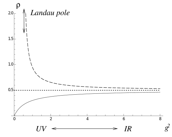
Figure 5: $\rho$ versus $g^{2}$. The dashed, dotted and solid lines correspond to the cases $c<0$, $c=0$, $c>0$ respectively.

Figure 5 also exhibits the pattern of the UV behavior. If $c$ is positive, $\rho$ is asymptotically free. For negative $c$ one hits the Landau pole at a large (but finite) value of the normalization point. Below we will not consider this regime because of its inconsistency. If we take $c=0$ the value for $\rho$ freezes at $\rho_{*}=1/2$ in the weak coupling domain, and, formally, remains at $1/2$ in the strong coupling domain too. As we will see later, in the heterotic CP$(N-1)$ models with $N>2$, the boundary value $\rho=1/2$ is a special point where a certain chiral flavor symmetry is restored.

8 Extension to CP$(N-1)$ with $N>2$

In this section, we will generalize our analysis to the heterotic CP$(N-1)$ sigma model. We will show that the parameter $\rho$ does not scale with $N$, and for any $N$ the function $\beta_{\rho}$ is the the same as in Eq. (50) at one loop. Then we will discuss a chiral fermion symmetry of the $\psi_{L}$’s sector at $\rho=1/2$, which will give us an argument that $\beta_{\rho}$ is proportional to $2\rho-1$ in all loops.

The heterotic CP$(N-1)$ Lagrangian in the geometric formulation can be borrowed from [7],

$$\mathcal{L}_{\text{CP}(N-1)} =G_{i\bar{j}}\left[\partial^{\mu}\phi^{i}\partial_{\mu}\phi^{\dagger\bar{j}}+i\bar{\psi}^{\bar{j}}\not{D}\psi^{i}\right]$$ (53)

$$+i\zeta_{R}^{\dagger}\partial_{L}\zeta_{R}+\left[\gamma\zeta_{R}G_{i\bar{j}}\left(i\partial_{L}\phi^{\dagger\bar{j}}\right)\psi_{R}^{i}+\text{H.c.}\right]+\gamma^{2}\left(\zeta_{R}^{\dagger}\zeta_{R}\right)\left(G_{i\bar{j}}\psi_{L}^{\dagger\bar{j}}\psi_{L}^{i}\right)$$

$$-\frac{g^{2}}{2}\left(G_{i\bar{j}}\psi_{R}^{\dagger\bar{j}}\psi_{R}^{i}\right)\left(G_{k\bar{m}}\psi_{L}^{\dagger\bar{m}}\psi_{L}^{k}\right)$$

$$+\frac{g^{2}}{2}\left(1-2\frac{\gamma^{2}}{g^{2}}\right)\left(G_{i\bar{j}}\psi_{R}^{\dagger\bar{j}}\psi_{L}^{i}\right)\left(G_{k\bar{m}}\psi_{L}^{\dagger\bar{m}}\psi_{R}^{k}\right)\,.$$

We again apply the phase rotation of $\gamma$ to make it real. Moreover, $G_{i\bar{j}}$ in Eq. (53) is the standard Käler metric in the Fubini–Study form. It is seen that $\rho=1/2$ is a special value nullifying the last line in Eq. (53). The scaling of the coupling constants with $N$ is as follows [21]:

$$g^{2}\sim N^{-1}\,,\quad\gamma^{2}\sim N^{-1}\,,\quad\rho\sim N^{0}\,.$$ (54)

Now we will establish that the $\beta$ functions $\beta_{g,\gamma}$ are compatible with the above scaling.

Our background field strategy can still be applied here much in the same way as in CP(1). As well known, in the undeformed model one has (e.g. [22])

$$\beta_{g}=-\frac{Ng^{4}}{4\pi}\,.$$ (55)

As was demonstrated in Sec. 4 (see also Appendix B), $\beta_{g}$ remains intact at one loop in the deformed model. Parallelizing our previous analysis it is not difficult to get that

$$Z_{\zeta}=1+i(N-1)\gamma^{2}I\,,\qquad Z_{\psi}=1+i\gamma^{2}I\,,$$ (56)

implying

$$\beta_{\gamma}=\frac{N\gamma}{4\pi}\left(\gamma^{2}-g^{2}\right)\,.$$ (57)

Finally, combining Eqs. (55) and (57) we conclude that in the heterotic CP$(N-1)$ model

$$\beta_{\rho}=\frac{Ng^{2}}{4\pi}\rho(2\rho-1)\,.$$ (58)

Thus, the scaling laws Eq. (54) indeed go through Eqs. (55), (57), and (58). Moreover, one can introduce the ’t Hooft couplings

$$\lambda=Ng^{2}\,,\qquad\gamma^{\prime}=\sqrt{N}\gamma\,,$$ (59)

in terms of which there are no explicit $N$ factors in the $\beta$ functions. In particular,

$$\beta_{\rho}=\frac{\lambda}{4\pi}\rho(2\rho-1)\,,\qquad\rho=\frac{\lambda}{\left(\gamma^{\prime}\right)^{2}}\,.$$ (60)

All UV and IR regimes observed in CP(1) are maintained in the heterotic CP$(N-1)$, in particular, the fixed point $\rho=1/2$. Note that the constant $c$ expressing the boundary condition in the solution Eq. (52) must be rescaled in CP$(N-1)$, namely,

$$\rho(g^{2})=\frac{1}{2+\frac{c}{Ng^{2}}}\,,$$ (61)

Now, after we dealt with arbitrary values of $N$, it is time to turn to the issue of the chiral fermion symmetry. A quick inspection of the third and fourth lines in Eq. (53) prompts us that their chiral structure is different. The third line is invariant under independent SU$(N-1)$ rotations of $\psi_{L}^{i}$ and $\psi_{R}^{j}$, while the fourth line is not. A class of rotations we keep in mind is the SU$(N-1)$ rotations of $\psi_{L}$’s, with $\psi_{R}$’s, $\zeta_{R}$, and bosonic fields intact. In the geometric formulation one introduces vielbeins $E^{a}_{i}$ and rotates

$$E^{a}_{i}\,\psi^{i}_{L}\to U^{a}_{b}\,E^{b}_{i}\,\psi^{i}_{L}\,\qquad E^{a}_{i}\,\psi^{i}_{R}\to E^{a}_{i}\,\psi^{i}_{R}\,,$$ (62)

where $U^{a}_{b}$ is a matrix from SU$(N-1)$. A similar transformation law can be written in the gauge formulation [7, 21] too. Note that in the CP(1) model the only possible chiral transformation of fermions is U(1), and it is anomalous. Hence, in fact there is no such symmetry. It starts from $N\geq 2$ in which case the chiral transformation is non-Abelian and nonanomalous. Consideration of the chiral fermion symmetries in the heterotic CP$(N-1)$ model was started by Tong [23].

At $\rho=1/2$ the fourth line in Eq. (53) vanishes. Other terms in the Lagrangian are invariant under the SU$(N-1)$ rotations of the left-handed fermions Eq. (62). (For the kinetic term of $\psi_{L}$’s see the discussion in Appendix D.)

Thus, at $\rho=1/2$ the symmetry of the heterotic CP$(N-1)$ Lagrangian is enhanced. It seems likely that this enhancement (and, hence, the fixed point at $\rho=1/2$ which goes with it) will hold to all orders in the coupling constant. Indeed, if one remembers about the origin of the heterotic CP$(N-1)$ model as the world-sheet theory on the strings supported in $\mu A^{2}$ deformed ${\mathcal{N}}=2$ SQCD, one can try to relate the above symmetry enhancement at $\rho=1/2$ with that in the bulk theory [23]. In the limit $\mu\to\infty$ the bulk theory becomes ${\mathcal{N}}=1$ SQCD acquiring a chiral symmetry absent at finite $\mu$. Remarkably, the $\mu\to\infty$ limit corresponds to $\rho\to 1/2$ on the world sheet [8, 9]. Thus, we expect the $\beta$ function $\beta_{\rho}$ to be proportional to $2\rho-1$ to all orders. We plan to explore this issue in more detail in [17].

Now we would like to argue that the solution Eq. (61) is, in fact, valid to all orders in perturbation theory in the (planar) limit of large $N$, and so is Eq. (58) for $\beta_{\rho}$. Indeed, the heterotic CP$(N-1)$ model was solved in the large-$N$ (planar) limit [10]. The heterotic deformation parameter determining a number of physical quantities (e.g. the vacuum energy density) is [10]

$$u=\frac{\rho}{(1-2\rho)\,(Ng^{2})}\,;$$ (63)

it must be renormalization-group invariant. In addition, $u$ does not scale with $N$. Substituting the solution Eq. (61) in Eq. (63) we indeed get

$$u=\frac{1}{c}\,,$$ (64)

quod erat demonstrandum. The normalization-point independence and $N^{0}$ scaling law are explicit in Eq. (64).

9 Conclusions

In this paper we started the study of perturbation theory in the recently found $\mathcal{N}=(0,2)$ CP$(N-1)$ sigma models. We carried out explicit calculations of both relevant $\beta$ functions at one loop and demonstrated that the theory is asymptotically free much in the same way as the unperturbed $\mathcal{N}=(2,2)$ CP$(N-1)$ models provided the initial condition for $\gamma^{2}$ is chosen in a self-consistent way (i.e. $c$ is positive). The $\beta$ function for the ratio $\rho=\gamma^{2}/g^{2}$ exhibits an IR fixed point at $\rho=1/2$. Formally this fixed point lies outside the validity of the one-loop approximation. We argued, however, basing on additional considerations, that the fixed point at $\rho=1/2$ may survive to all orders. The reason is the enhancement of symmetry (restoration of a chiral fermion flavor symmetry) at $\rho=1/2$. Moreover, we argued that Eq. (61) for $\beta_{\rho}$ formally obtained at one loop, is in fact exact to all orders in the large-$N$ (planar) approximation. Thus, in this approximation the fixed point at $\rho=1/2$ is firmly established.

In addition to the above quantitive results, we also got insights on field-theoretical aspects of the heterotic model. Using the $\mathcal{N}=(0,2)$ superfield language, we saw that in CP(1) both fields $\psi_{R}$ and $\zeta_{R}$ get the same renormalization at one loop level. This is due to an unexpectated and unusual SU$(2)$ symmetry between $\psi_{R}$ and $\zeta_{R}$. The novelty of this symmetry is quite obvious because it mixes chiral and anti-chiral superfields, and does not commute with the target space symmetry.

Appendix A

In this appendix we describe the $\mathcal{N}=(0,2)$ superspace in $D=1+1$ dimensions, present our notation, and derive Eq. (12).

The space-time coordinate $x^{\mu}=\{t,z\}$ can be promoted to superspace by adding a complex Grassmann variable $\theta_{R}$ and its complex conjugate $\theta_{R}^{\dagger}$. Where-ever our expressions are dependent on the representation of Clifford algebra, we use the following convention.

$$\gamma^{0}=\left(\begin{smallmatrix}0&-i\\ i&0\end{smallmatrix}\right)\,,\qquad\gamma^{1}=\left(\begin{smallmatrix}0&i\\ i&0\end{smallmatrix}\right)\,,\qquad\gamma^{3}=\gamma^{0}\gamma^{1}=\left(\begin{smallmatrix}1&0\\ 0&-1\end{smallmatrix}\right)\,.$$ (A.1)

Under this representation Dirac fermion is expressed as

$$\psi=\left(\begin{smallmatrix}\psi_{R}\\ \psi_{L}\end{smallmatrix}\right)\,,$$ (A.2)

and we have

$$\not{\partial}=\left(\begin{smallmatrix}0&-i\partial_{R}\\ i\partial_{L}&0\end{smallmatrix}\right)\,,$$ (A.3)

where $\partial_{R}=\partial_{t}-\partial_{z}$ and $\partial_{L}=\partial_{t}+\partial_{z}$. The corresponding supercharges are given by

$$Q_{R}=i\frac{\partial}{\partial\theta_{R}}-\theta_{R}^{\dagger}\partial_{L}\,,\qquad\bar{Q}_{R}=\frac{\partial}{\partial\theta_{R}^{\dagger}}+i\theta_{R}\partial_{L}\,.$$ (A.4)

Applying them to the superspace, we have the transformation rules as follow.

$$i(Q_{R}\epsilon_{R}+\bar{\epsilon}_{R}\bar{Q}_{R})x^{\mu}=i\epsilon_{R}^{\dagger}\theta_{R}-i\theta_{R}^{\dagger}\epsilon_{R}\,,$$

$$i(Q_{R}\epsilon_{R}+\bar{\epsilon}_{R}\bar{Q}_{R})\theta_{R}=\epsilon_{R}\,,\qquad i(Q_{R}\epsilon_{R}+\bar{\epsilon}_{R}^{\dagger}\bar{Q}_{R})\theta_{R}^{\dagger}=\epsilon_{R}^{\dagger}\,,$$ (A.5)

where $\mu\in\{0,1\}$, $\bar{\epsilon}_{R}=-i\epsilon_{R}^{\dagger}$. So in fact if we define

$$x_{L}^{\mu}=x^{\mu}+i\theta_{R}^{\dagger}\theta_{R}\,\,\mbox{ and}\,\,x_{R}^{\mu}=x^{\mu}-i\theta_{R}^{\dagger}\theta_{R}\,,$$

then we have

$$i(Q_{R}\epsilon_{R}+\bar{\epsilon}_{R}\bar{Q}_{R})x_{L}^{\mu}=2i\epsilon_{R}^{\dagger}\theta_{R}\,,\qquad i(Q_{R}\epsilon_{R}+\bar{\epsilon}_{R}\bar{Q}_{R})x_{L}^{\mu}=-2i\theta_{R}^{\dagger}\epsilon_{R}\,.$$ (A.6)

Now we are ready to deduce the transformation law for the chiral superfield $A$ and $B$.

$$i(Q_{R}\epsilon_{R}+\bar{\epsilon}_{R}\bar{Q}_{R})[\phi(x_{L})+\sqrt{2}\theta_{R}\psi_{L}(x_{L})]=\partial_{L}\phi 2i\epsilon_{R}^{\dagger}\theta_{R}+\sqrt{2}\epsilon_{R}\psi_{L}\,,$$

$$i(Q_{R}\epsilon_{R}+\bar{\epsilon}_{R}\bar{Q}_{R})[\psi_{R}(x_{L})+\sqrt{2}\theta_{R}F(x_{L})]=\partial_{L}\psi_{R}2i\epsilon_{R}^{\dagger}\theta_{R}+\sqrt{2}\epsilon_{R}F\,.$$ (A.7)

And this immediately leads us to Eq. (12).

Finally, we comment that for the chiral superfield $A$, we have that $\partial_{R}A$ is also a chiral superfield. This is because of the fact that $[Q_{R},\partial_{R}]=[\bar{Q}_{R},\partial_{R}]=0$.

Appendix B

In the limit of small $m$ the one-loop fermion contribution is determined by the diagram depicted in Fig. 6.

Figure 6: One-loop contribution by fermionic loop. The solid lines denote fermionic propagators, and the wave lines are bosonic background fields.

Let us start from $m=0$. Then the fermion Green’s function is

$$\left\langle T\,\psi(x)\,\bar{\psi}(0)\right\rangle=-\frac{i}{2\pi}\frac{\not{x}}{x^{2}}\,.$$ (B.1)

Correspondingly,

$$\left\langle T\,\bar{\psi}(x)\gamma^{\mu}\psi(x)\,\,\bar{\psi}(0)\gamma^{\nu}\psi(0)\right\rangle = \frac{1}{2\pi^{2}}\left(x^{2}g^{\mu\nu}-2x^{\mu}x^{\nu}\right)\frac{1}{x^{4}}$$ (B.2)

$$\to \frac{i}{\pi}\left(\frac{p^{\mu}p^{\nu}}{p^{2}}-g^{\mu\nu}\right).$$

This expression is singular at $p\to 0$. However, if we keep a small IR regularizing mass, then it must be multiplied by a function $f(p^{2}/m^{2})$ which is proportional to $p^{2}/m^{2}$ at small $p^{2}$. Thus the fermion loop in Fig. 6 vanishes at $p\to 0$.

Appendix C

In order to simplify the calculation, we only collect the covariant contribution, and take the target space symmetry of the theory for granted. First we calculate one-loop correction to $(\bar{\psi}\psi)^{2}$. The relevant diagrams are shown in Fig. 7.

Figure 7: One-loop corrections to $(\bar{\psi}\psi)^{2}$ term.

Finally we have

$$\Delta\mathcal{L}_{(\bar{\psi}\psi)^{2}}=i\frac{2}{(1+\phi^{\dagger}\phi)^{4}}(-1+\frac{\gamma^{2}}{g^{2}}+\frac{\gamma^{4}}{g^{4}})I(\bar{\psi}\psi)^{2}\,.$$ (C.1)

In order to see whether there are new structures, we recall that previously we have

$$\mathcal{L}_{0,(\bar{\psi}\psi)^{2}}=\frac{2}{g_{0}^{2}(1+\phi^{\dagger}\phi)^{4}}(\bar{\psi}_{0}\psi_{0})^{2}-\frac{2\gamma_{0}^{2}}{g_{0}^{4}(1+\phi^{\dagger}\phi)^{4}}(\bar{\psi}_{0}\psi_{0})^{2}\,.$$ (C.2)

So if the structure remains the same after one-loop renormalization, we should have

$$\mathcal{L}_{\text{eff},(\bar{\psi}\psi)^{2}} = \frac{2}{g^{2}(1+\phi^{\dagger}\phi)^{4}}(\bar{\psi}\psi)^{2}-\frac{2\gamma^{2}}{g^{4}(1+\phi^{\dagger}\phi)^{4}}(\bar{\psi}\psi)^{2}$$ (C.3)

$$= Z_{g^{2}}^{-1}Z_{\psi}\frac{2}{g_{0}^{2}(1+\phi^{\dagger}\phi)^{4}}(\bar{\psi}_{0}\psi_{0})^{2}-Z_{\frac{\gamma}{g^{2}}}^{2}Z_{\psi}\frac{2\gamma_{0}^{2}}{g_{0}^{4}(1+\phi^{\dagger}\phi)^{4}}(\bar{\psi}_{0}\psi_{0})^{2}\,,$$

where

$$Z_{g^{2}}=\frac{g^{2}}{g_{0}^{2}}=1+iIg^{2}\,,\qquad Z_{\frac{\gamma}{g^{2}}}=\frac{\gamma g_{0}^{2}}{\gamma_{0}g^{2}}=1-iI\gamma^{2}\,,$$

$$Z_{\psi}=1+iI\gamma^{2}\,.$$ (C.4)

The last one is because $\bar{\psi}\psi$ is linear in $\psi_{R}$(or $\psi_{R}^{\dagger}$). So if we plug in Eq. (C.3) the known result Eq. (C.4), we should expect that

$$\Delta\mathcal{L}_{(\bar{\psi}\psi)^{2}}=i\frac{2}{(1+\phi^{\dagger}\phi)^{4}}(-1+\frac{\gamma^{2}}{g^{2}}+\frac{\gamma^{4}}{g^{4}})I(\bar{\psi}\psi)^{2}\,.$$ (C.5)

And it is precisely the case.

We can also calculate one-loop correction to $\zeta_{R}^{\dagger}\zeta_{R}\psi_{L}^{\dagger}\psi_{L}$, and the relevant diagrams are given in Fig. 8.

Figure 8: One-loop corrections to $\zeta_{R}^{\dagger}\zeta_{R}\psi_{L}^{\dagger}\psi_{L}$ term.

Finally we have

$$\Delta\mathcal{L}_{\zeta_{R}^{\dagger}\zeta_{R}\psi_{L}^{\dagger}\psi_{L}}=i\frac{2}{(1+\phi^{\dagger}\phi)^{2}}\frac{\gamma^{2}}{g^{2}}(g^{2}-\gamma^{2})I\zeta_{R}^{\dagger}\zeta_{R}\psi_{L}^{\dagger}\psi_{L}\,.$$ (C.6)

Following a similar analysis one can show that this is also consistent with our expectation.

Appendix D

In this appendix we introduce vielbeins $E_{i}^{a}$, used in Sec. 8 to describe the flavor symmetry of the left-handed fermions $\psi_{L}$. The $\psi$ fermions live in the tangent space of the target manifold. Vielbeins make it clear that locally we could find a coordinate frame that is as good as the one for flat spaces. However, such choice of coordinates varies from point to point, so one should expect that the fermions have nontrivial connections.

Let us look at the fermionic part of the Lagrangian, which is given by Eq. (53). It is convenient to write the Kähler metric as $G_{\bar{j}i}$. Then all vectors that carry the barred indices must be understood as lines, and all that carry the unbarred indices as columns. We consider the following representation of the metric:

$$\left(E^{\dagger}\right)^{a}_{\bar{j}}E_{a,i}=G_{\bar{j}i}\,.$$ (D.1)

Rising or lowering of the $a$ index is done by the identity matrix, so we can be loose about its position. The above equation does not uniquely determine the matrix $E$. Rather, we start with $(N-1)\times(N-1)$ complex matrix and impose $(N-1)^{2}$ real conditions. The remaining freedom (the ambiguity can be represented by a constant U$(N-1)$ matrix) is non-physical and one can fix the ambiguity by imposing further compatible conditions. After that, we can define our “flat” fermions as

$$\psi^{a}=E_{i}^{a}\psi^{i}\,.$$ (D.2)

On the other hand, in any case the kinetic term for fermions needs some adjustments. Previously we had $\not{D}\psi^{i}\equiv\not{\partial}\psi^{i}+\Gamma^{i}_{lk}\not{\partial}\phi^{l}\psi^{k}$, and now, in order to require the covariant derivatives to be the same both before and after we apply Eq. (D.2), we must have

$$\not{D}\psi^{a}=E_{i}^{a}\not{D}\psi^{i}\,.$$ (D.3)

These conditions determine that

$$D_{\mu}\psi^{a}=\partial_{\mu}\psi^{a}+\partial_{\mu}(E^{a}_{i})\psi^{i}-E_{i}^{a}\Gamma^{i}_{lk}\partial_{\mu}\phi^{l}\psi^{k}\,.$$ (D.4)

Generally speaking, it is impossible to choose the set of the vielbeins $E_{i}^{a}$ to reduce $D_{\mu}\psi^{a}$ to $\partial_{\mu}\psi^{a}$. The reason is simple: the change of local coordinate frames from one point on the target space to another is not trivial. In a sence, the U$(N-1)$ symmetries in choosing $E_{i}^{a}$’s are similar to a gauge symmetry.

The symmetry we demonstrate here, is seen by replacing $\psi^{i}$’s by $\psi^{a}$’s. Now the fermion part of the Lagrangian takes the form

$$\mathcal{L}_{\text{CP}(N-1)} =i\psi_{R}^{\dagger a}D_{L}\psi_{R}^{a}+i\psi_{L}^{\dagger a}D_{R}\psi_{L}^{a}$$ (D.5)

$$+i\zeta_{R}^{\dagger}\partial_{L}\zeta_{R}+\left[\gamma\zeta_{R}\left(i\partial_{L}\phi^{\dagger\bar{j}}E^{\dagger}_{\bar{j}a}\right)\psi_{R}^{a}+\text{H.c.}\right]+\gamma^{2}\left(\zeta_{R}^{\dagger}\zeta_{R}\right)\left(\psi_{L}^{\dagger a}\psi_{L}^{a}\right)$$

$$-\frac{g^{2}}{2}\left(\psi_{R}^{\dagger a}\psi_{R}^{a}\right)\left(\psi_{L}^{\dagger b}\psi_{L}^{b}\right)$$

$$+\frac{g^{2}}{2}\left(1-2\frac{\gamma^{2}}{g^{2}}\right)\left(\psi_{R}^{\dagger a}\psi_{L}^{a}\right)\left(\psi_{L}^{\dagger b}\psi_{R}^{b}\right)\,,$$

where $D_{R}$ and $D_{L}$ are defined from $D_{\mu}$ in the way similar to the replacement of $\partial_{\mu}$ by $\partial_{R}$ and $\partial_{L}$.

As was emphasized before, since $D_{L}$ and $D_{R}$ do not reduce to $\partial_{L}$ and $\partial_{R}$, we cannot yet apply the flavor rotation to $\psi_{L}^{a}$’s: the corresponding kinetic term in the Lagrangian will not be invariant. But it will be invariant, if we further assume that $\phi$’s are only dependent on $t+z$. By doing so, $D_{R}\to\partial_{R}$, since the connection part is always linear in $\partial_{R}\phi^{i}$’s. Now we can see that the last line in Eq. (D.5) is the only term that is noninvariant under the SU$(N-1)$ flavor rotation of $\psi_{L}^{a}$. Needless to say, the symmetry is restored when $\rho=1/2$.

References

• [1] A. Hanany and D. Tong, JHEP 0307, 037 (2003) [hep-th/0306150].
• [2] R. Auzzi, S. Bolognesi, J. Evslin, K. Konishi and A. Yung, Nucl. Phys. B 673, 187 (2003) [hep-th/0307287].
• [3] M. Shifman and A. Yung, Phys. Rev. D 70, 045004 (2004) [hep-th/0403149].
• [4] A. Hanany and D. Tong, JHEP 0404, 066 (2004) [hep-th/0403158].
• [5] D. Tong, Annals Phys.  324, 30 (2009) [arXiv:0809.5060 [hep-th]]; M. Eto, Y. Isozumi, M. Nitta, K. Ohashi and N. Sakai, J. Phys. A 39, R315 (2006) [arXiv:hep-th/0602170]; K. Konishi, Lect. Notes Phys.  737, 471 (2008) [arXiv:hep-th/0702102]; M. Shifman and A. Yung, Supersymmetric Solitons, (Cambridge University Press, 2009).
• [6] M. Edalati and D. Tong, JHEP 0705, 005 (2007) [arXiv:hep-th/0703045].
• [7] M. Shifman and A. Yung, Phys. Rev.  D 77, 125016 (2008) [arXiv:0803.0158 [hep-th]].
• [8] P. A. Bolokhov, M. Shifman and A. Yung, Phys.  Rev.  D 79, 085015 (2009) (Erratum: Phys. Rev. D 80, 049902 (2009)) [arXiv:0901.4603 [hep-th]].
• [9] P. A. Bolokhov, M. Shifman and A. Yung, Phys.  Rev.  D 79, 106001 (2009) (Erratum: Phys. Rev. D 80, 049903 (2009)) [arXiv:0903.1089 [hep-th]].
• [10] M. Shifman and A. Yung, Phys. Rev.  D 77, 125017 (2008) [Erratum-ibid.  D 81, 089906 (2010)] [arXiv:0803.0698 [hep-th]]; P. A. Bolokhov, M. Shifman and A. Yung, Phys. Rev.  D 82, 025011 (2010) [arXiv:1001.1757 [hep-th]].
• [11] P. Koroteev, A. Monin, and W. Vinci, Large-$N$ Solution of the Heterotic Weighted Sigma Model, to appear.
• [12] E. Witten, Two-dimensional models with $(0,2)$ supersymmetry: Perturbative aspects, arXiv:hep-th/0504078.
• [13] B. Zumino, Phys. Lett. 87B, 203 (1979).
• [14] E. Witten, Phys. Rev.  D 16, 2991 (1977).
• [15] N. Seiberg, Phys. Lett. 318, 469 (1993) [arXiv:hep-ph/9309335].
• [16] V. A. Novikov, M. A. Shifman, A. I. Vainshtein and V. I. Zakharov, Phys. Rept.  116, 103 (1984).
• [17] X. Cui and M. Shifman, work in progress.
• [18] A. M. Polyakov, Phys. Lett.  B 59, 79 (1975).
• [19] J. Chen, Instanton Fermionic Zero Modes of Heterotic CP(1) Sigma Model, arXiv:0912.0571 [hep-th].
• [20] M. A. Shifman and A. I. Vainshtein, Nucl. Phys.  B 277, 456 (1986).
• [21] P. A. Bolokhov, M. Shifman and A. Yung, Phys. Rev.  D 81, 065025 (2010) [arXiv:0907.2715 [hep-th]].
• [22] A. Y. Morozov, A. M. Perelomov and M. A. Shifman, Nucl. Phys.  B 248, 279 (1984).
• [23] D. Tong, JHEP 0709, 022 (2007) [arXiv:hep-th/0703235].