Atmospheric Phase Correction using CARMA-PACS: High Angular Resolution Observations of the FU-Orionis star PP 13S*

Abstract

We present $0.15^{\prime\prime}$ resolution observations of the 227 GHz continuum emission from the circumstellar disk around the FU-Orionis star PP 13S*. The data were obtained with the Combined Array for Research in Millimeter-wave Astronomy (CARMA) Paired Antenna Calibration System (C-PACS), which measures and corrects the atmospheric delay fluctuations on the longest baselines of the array in order to improve the sensitivity and angular resolution of the observations. A description of the C-PACS technique and the data reduction procedures are presented. C-PACS was applied to CARMA observations of PP 13S*, which led to a factor of 1.6 increase in the observed peak flux of the source, a 36% reduction in the noise of the image, and a 52% decrease in the measured size of the source major axis. The calibrated complex visibilities were fitted with a theoretical disk model to constrain the disk surface density. The total disk mass from the best fit model corresponds to 0.06 M_⊙, which is larger than the median mass of a disk around a classical T Tauri star. The disk is optically thick at a wavelength of 1.3 mm for orbital radii less than 48 AU. At larger radii, the inferred surface density of the PP 13S* disk is an order of magnitude lower than that needed to develop a gravitational instability.

1. Introduction

Electromagnetic waves from an astronomical radio source suffer distortion from irregularities in the refractivity of the atmosphere (Thompson et al., 2001). At millimeter and submillimeter wavelengths, the distortions are caused primarily by a turbulent water vapor distribution, though dry air turbulence may also be important under some circumstances (Stirling et al., 2006). The spatial scales of the turbulence extend to kilometer distances with a power law spectrum (Kolmogorov, 1941) that creates atmospheric delay fluctuations on timescales that range from fractions of a second to tens of minutes. The signal degradation is particularly serious for millimeter-wave radio interferometers in extended configurations, where perturbation of phases across the instrument often exceeds many radians. These perturbations can lead to decorrelation (loss of amplitude), distortion of the image, and loss of resolution (Lay, 1997).

Different approaches have been employed to overcome the effect of atmospheric delay fluctuations. A straightforward approach is self-calibration (Schwab, 1980), where the visibility phase used to calibrate the data is measured from the actual science target. A model for the source spatial structure is needed and bright sources are required to measure the fringe phase with a high signal to noise ratio in a short integration. Two other approaches have been applied to faint targets. In water vapor radiometry (Westwater, 1967; Woody et al., 2000), a dedicated radiometer monitors the water vapor emission along the pointing direction of the antenna. In fast position switching (Holdaway et al., 1995), the antennas switch rapidly between the science target and a nearby phase calibrator to capture the atmospheric delay fluctuations on time scales longer than the switching cycle time. Both methods probe the atmosphere close to the line-of-sight toward the science target, but have limitations in actual applications. Fast position switching reduces the time spent on source by a factor of $\sim 2$, while water vapor radiometry requires a physical model to relate the water line brightness and the path correction, as well as it assumes that refractivity fluctuations are produced only by water vapor.

As an alternative approach, an array of closely paired antennas (Asaki et al., 1996, 1998) continuously monitors the atmospheric phase fluctuations by observing a nearby calibrator. Two arrays of antennas are necessary: antennas belonging to the “science array” observe the science target and phase calibrator, while antennas belonging to the “reference array” simultaneously monitor an atmospheric calibrator. Phase correction on the science target and phase calibrator is accomplished by subtracting the visibility phase measured from the atmospheric calibrator on each baseline. An advantage of the paired antenna technique over water vapor radiometry is that it accounts for atmospheric phase fluctuations due to both water vapor and a dry air component.

Between November 2008 and February 2009, the Combined Array for Research in Millimeter-wave Astronomy (CARMA) implemented the CARMA Paired Antenna Calibration System (C-PACS) to correct for atmospheric delay fluctuations on the longest baselines of the interferometer (up to 2 km in length). The goal of C-PACS is to enable routine imaging in the most extended CARMA configurations.

In this paper we describe C-PACS and apply this calibration technique to observations of the circumstellar dust around PP 13S*. PP 13S* is a young pre-main sequence star located in the constellation of Perseus and embedded in the L1473 dark cloud at a distance of $\sim$ 350 pc (Cohen et al., 1983). This object is thought to have experienced a FU-Orionis-type outburst in the past due to a massive accretion episode and is now declining in brightness to a quiescent state (Aspin & Sandell, 2001). The FU-Orionis nature of PP 13S* has been established based on the highly broadened infrared CO absorption bands (Sandell & Aspin, 1998), the jet-like feature seen in [SII] emission which is characteristic of Herbig-Haro outflows (Aspin & Reipurth, 2000; Aspin & Sandell, 2001), and the consistent dimming and morphology changes observed at near-IR and optical wavelengths over several decades (Aspin & Sandell, 2001). All of these characteristics are common to FU-Orionis objects (Hartmann & Kenyon, 1996). The star, with a bolometric luminosity of 30 L_⊙ (Cohen et al., 1983), is surrounded by an extended disk and envelope that contains about 0.6 M_⊙ of gas and dust (Sandell & Aspin, 1998). The new CARMA observations will help understand the origin of the FU-Orionis phenomena in PP 13S* by measuring the distribution of dust continuum emission on spatial scales of $\sim 50$ AU.

2. Description of C-PACS

Before presenting the new observations of PP 13S*, we describe the paired antenna calibration system as implemented at CARMA. We first describe the antenna configuration used for the observations, and outline the basic principles of the technique.

2.1. CARMA

CARMA is an heterogeneous interferometer comprising 23 antennas: six 10.4-m telescopes from the California Institute of Technology/Owens Valley Radio Observatory (OVRO), nine 6.1 m telescopes from the Berkeley-Illinois-Maryland Association (BIMA), and eight 3.5-m telescopes from the University of Chicago Sunyaev-Zel’dovich Array (SZA). The two most extended array configurations contain baselines that range in length from 100 m to 1000 m (B configuration) and 250 m to 1900 m (A configuration) to achieve an angular resolution of 0.3″ and 0.15″ respectively, at an observing frequency of 230 GHz.

A schematic of C-PACS is shown in Figure 1. C-PACS pairs the eight 3.5-m antennas with selected 6-m and 10-m antennas, preferentially on the longer baselines. Typically, a 3.5-m antenna is offset by 20–30 m to the west of a larger antenna. This separation is a compromise between the need to put the antennas as close as possible to probe the same atmospheric path and to avoid shadowing between antennas.

The science array, composed of the 6-m and 10-m antennas, operates in the 1.3- or 3-mm atmospheric windows as requested by the investigator. The reference array, comprising the 3.5-m antennas, operates in the 1-cm window. The observing cycle consists of observations of the science target interleaved with periodic observations of the phase calibrator. Both the science and reference arrays observe the phase calibrator to measure instrumental phases drifts. Subsequently, the science array observes the science target while the reference array monitors a strong point source (i.e., the “atmospheric” calibrator) close to the science target, to measure the delay introduced by the atmosphere. The atmospheric delay measured by the 3.5-m antennas can then be applied to the science observations.

2.2. Properties of the atmosphere

It is helpful to have a physical picture to understand the principles of the correction. We suppose the atmosphere to be a pattern of random refractive index variations that is blown across the array at the wind velocity. Furthermore, we assume that the layer is at a height of a couple of kilometers and that the thickness is much less than the height. General experience at this and other sites show that these conditions are often consistent with what is observed. Other conditions can be present, but can often be characterized by two or more layers at different altitudes with separate wind vectors so that only a small change to the analysis is required.

Kolmogorov theory predicts a turbulence distribution with a power law spectrum from less than a millimeter in size to many kilometers. This results in random delay differences between signals arriving at different antennas that increase with separation as a power law function (Tatarskii, 1961). As the pattern moves over the array, the delay differences are observed as temporal fluctuations in the visibility phases. The RMS of the delay depends on the wind speed, but not its direction. Structures smaller in size than the antenna diameter are averaged out and do not contribute to the phase errors. Structures on scales large in comparison with the baseline length are common to the two antennas on the baseline and therefore tend to cancel out. From these theoretical considerations supported by experimental evidence (Sramek, 1983, 1989), it is found that the resulting delay variance vs baseline length (i.e., the delay structure function) also follows a power-law. The theoretical slope of the power-law is 5/3 and 2/3 for two- and three-dimensional Kolmogorov turbulence, respectively.

2.3. Atmospheric delay corrections

Following the discussion in Asaki et al. (1996), consider two pairs of antennas as shown in Figure 1. In the simplest case, we measure the delay difference between the antennas on the reference baseline (i.e., baseline $A_{3}-A_{4}$ in Figure 1) as a function of time. Assuming a non-dispersive atmosphere, the delay on the science baseline (i.e., baseline $A_{1}-A_{2}$) is corrected by applying the delay difference on the reference baseline to the visibility measurement.

The reference and science delays are not identical since the two baselines are not exactly co-located. The relevant distances that determine the efficacy of the delay corrections are not the baseline lengths at the ground, but the distances between the radio beams as they traverse the turbulent layer (i.e. $A_{1}^{\prime}-A_{3}^{\prime}$ and $A_{2}^{\prime}-A_{4}^{\prime}$ in Figure 1). The beam separation at the turbulent layer depends upon the relative positions of the target and reference source in the sky, the height of the turbulent layer, and the configuration of the antennas on the ground. The upper limit to the beam separation is given by

$$d_{\mathrm{max}}=|A_{1}-A_{2}|+\alpha h/sin(e),$$ (1)

where $\alpha$ is the angular separation between the science target and the atmospheric calibrator, $h$ the height of the turbulence, and $e$ is the source elevation. Assuming that the turbulent layer is at a height of 1 km (continuous line) or at 2 km (dashed line), Figure 2 shows the trajectories of the 3.5-m beam locations relative to the 6-m and 10-m beams for an 8 h observation of PP 13S* centered on transit with 3C111 as the atmospheric calibrator. As shown in this figure, the choice of 3C111 as the atmospheric calibrator is particularly fortuitous for PP 13S* since the science and reference beams for most antennas nearly cross within the turbulent zone.

Using phase closure (Jennison, 1958), the difference ($\Delta\tau$) between the actual delay for the target beams $A_{1}^{\prime}-A_{2}^{\prime}$ and the atmospheric reference beams $A_{3}^{\prime}-A_{4}^{\prime}$ is given by $\Delta\tau=\tau(A_{1}^{\prime}-A_{2}^{\prime})-\tau(A_{3}^{\prime}-A_{4}^{\prime})=\tau(A_{1}^{\prime}-A_{3}^{\prime})-\tau(A_{2}^{\prime}-A_{4}^{\prime})$. In a favorable configuration, the beam separations $A_{1}^{\prime}-A_{3}^{\prime}$ and $A_{2}^{\prime}-A_{4}^{\prime}$ will be much less than either the target beam separation $A_{1}^{\prime}-A_{2}^{\prime}$ or the reference beam separation $A_{3}^{\prime}-A_{4}^{\prime}$. The RMS of the corrected visibilities will be $\sqrt{2}$ worse than for an array with beam separation $A_{1}^{\prime}-A_{3}^{\prime}$, which implies that C-PACS will have a performance equivalent to an array that has baseline lengths $\sim$20–70% larger than the $A_{1}^{\prime}-A_{3}^{\prime}$ beam separation, depending on the structure function exponent. The complete analysis contains additional correlation terms and added uncertainties caused by the finite signal-to-noise for the atmospheric calibrator observations.

2.4. Atmospheric calibrators

The ability of C-PACS to correct the atmospheric delays is limited by the delays from the short beam spacings $A_{1}^{\prime}-A_{3}^{\prime}$ and $A_{2}^{\prime}-A_{4}^{\prime}$ (see Figure 1), instrumental phase drifts on the reference array, and the radiometer noise. The delay errors caused by differences in the beam spacings between the science and reference arrays are given statistically by the structure function $R(|A_{i}^{\prime}-A_{j}^{\prime}|)$. The instrumental errors can be removed by removing a box-car average over the length of the observation, and will contribute negligible delay errors as long as the timescale for the instrumental drifts are large compared to the box-car width. The delay errors due to radiometric phase noise depend on the strength of the source being observed, the receiver properties, and the atmospheric characteristics (Thompson et al., 2001). The uncertainty in the measured phase from radiometer noise is given by

$$\Delta\phi=\frac{\sqrt{2}k_{\mathrm{B}}T_{\mathrm{sys}}}{\eta_{Q}A_{\mathrm{eff}}S\sqrt{Bt}}$$ (2)

where $k_{\mathrm{B}}$ is the Boltzmann’s constant, $T_{\mathrm{sys}}$ is the system temperature, $\eta_{Q}$ is the correlator quantization efficiency, $A_{\mathrm{eff}}$ is the effective collecting area of the antennas, $S$ is the flux density of the atmospheric calibrator, $B$ is the bandwidth of the observations, and $t$ is the integration time. The measurement uncertainty in the delay is then $\Delta\phi/(2\pi\nu)$. The net variance in the delay after applying C-PACS is given by

$$\Delta\tau^{2}\approx R(|A_{1}^{\prime}-A_{3}^{\prime}|)+R(|A_{2}^{\prime}-A_{4}^{\prime}|)+\Bigl{(}{k_{B}T_{\mathrm{sys}}\over\eta_{Q}A_{\mathrm{eff}}S\pi\nu\sqrt{2Bt}}\Bigr{)}^{2}$$ (3)

The structure function is generally described by a power law with exponents varying from 5/3 to 2/3 depending upon the spacing and thickness of the turbulent layer. The scaling coefficient of the power law also varies depending upon the weather conditions. In order for C-PACS to improve the image quality, the target and reference beams must be close at the turbulent layer such that $R(|A_{1}^{\prime}-A_{3}^{\prime}|)+R(|A_{2}^{\prime}-A_{4}^{\prime}|)\ll\lambda^{2}$. This requires angular separations $\mathbin{\lower 3.0pt\hbox{$\hbox to0.0pt{\raise 5.0pt\hbox{$\char 60\relax$}\hss}\mathchar 29208\relax$}}$ 5° for the A and B configuration C-PACS pairings and typical winter weather conditions at the CARMA site. A future publication will use actual measurements to quantify how the quality of the C-PACS correction varies with angular separation between the science target and the atmospheric calibrator (Zauderer et al., in preparation).

The radiometer noise should also contribute much less than a wavelength of delay error for the C-PACS corrections to be successful. For the characteristics of the 3.5-m telescopes and the 1-cm receivers, the radiometer delay error is given by

$$\Delta\tau_{\mathrm{radiometer}}=1.3\mathrm{mm}\,\Bigl{(}{S_{\nu}\over\mathrm{1Jy}}\Bigr{)}^{-1}\,\Bigl{(}{t\over\mathrm{1s}}\Bigr{)}^{-1/2}$$ (4)

Thus, 1.3-mm observations with integration times of $t=4$ s (short enough to measure and correct most of the atmosphere fluctuations) require a reference source brighter than $S\sim 1$ Jy in the 1 cm band. When several atmospheric calibrators are available, the optimum choice between calibrator separation and brightness can be found by minimizing Equation 3 for the expected weather conditions.

We combined the SZA 30 GHz calibrator list, the GBT catalog at 1.4 and 5.0 GHz (Condon & Yin, 2001), and the WMAP point source catalog (Wright et al., 2009) to estimate the density of potential C-PACS calibrators. For each source in the GBT catalog, we extrapolated the flux density from 5.0 GHz to 30 GHz by measuring the spectral index $\alpha$ between 1.4 and 5.0 GHz ($S_{\nu}\propto\nu^{\alpha}$). We find that $50\%$ of the sky is within $5\arcdeg$ of a point source with flux density greater than $1$ Jy at 30 GHz. The number of suitable C-PACS calibrators could be expanded by increasing the sensitivity of the reference array, which would allow us to employ fainter atmospheric calibrators. This could be accomplished by increasing the correlator bandwidth or improving the receiver sensitivity.

3. Observations and Data Reduction

PP 13S* is particularly well suited for C-PACS observations since the nearest atmospheric calibrator (3C111) is bright ($\sim$ 4 Jy at 1.3 mm at the time of the observations) and separated by 1.5° from PP 13S*. Thus the calibrator satisfies the basic criteria needed for successful C-PACS corrections (see Section 2.4). In this section, we describe the CARMA observations and data reduction of PP 13S*.

3.1. CARMA 1.3-mm wavelength observations

The 6-m and 10-m antennas were used to obtain 1.3 mm continuum observations of PP 13S* on UT Dec 5, 2008 in the CARMA B configuration and on UT Jan 18, 2009 in the CARMA A configuration. Double-sideband receivers mounted on each antenna were tuned to a rest frequency of 227 GHz placed in the upper sideband. The correlator was configured with three 468.75 MHz wide bands to provide 1.41 GHz of continuum bandwidth per sideband. The observing sequence interleaved 3 min observations of 3C111 with 12 min observations of PP 13S* in B configuration and 4 min in A configuration. The complex visibilities were recorded every 4 s.

Data reduction was performed using the Multichannel Image Reconstruction, Image Analysis and Display (MIRIAD) software package (Sault et al., 1995). Each night of observations was calibrated separately. The calibration consisted of first applying a line-length correction and then a passband correction derived from observations of 3C111. Only these two calibrations were applied to the millimeter data before proceeding with the C-PACS corrections (see Section 3.3). All images that are presented here were formed by inverting the visibility data using natural weighting, and then “cleaning” with the point spread function (i.e. the “dirty” beam) using a hybrid Högbom/Clark/Steer algorithm (Högbom, 1974; Clark, 1980; Steer, Dewdney, & Ito, 1984).

3.2. CARMA 1-cm wavelength observations

The eight 3.5-m antennas were used to obtain 1-cm observations of the atmospheric calibrator simultaneously with the 1.3-mm wavelength observations. Single-sideband receivers mounted on each antenna were tuned to a sky center frequency of 30.4 GHz. For these antennas, a wideband correlator is available that was configured with fourteen 500 MHz wide bands to provide 7 GHz of continuum bandwidth. Complex visibilities were recorded every 4 s in order to track the rapidly varying atmospheric fluctuations. Single-sideband system temperatures for the 1-cm observations ranged between 35 and 55 K.

The data calibration consisted of applying a time-dependent passband measured from an electronically correlated noise source that was observed every 60 s. This passband was computed and applied on a 60 s timescale to remove any delay variations in the digitizers due to temperature cycling of the air-conditioning that cools the correlator. A passband correction derived from observations of 3C111 was then applied.

3.3. Applying 1-cm delays to the 1.3-mm data

Phase referencing would normally be performed at this point in the data reduction process to remove the slowly varying phase drift introduced by the instrument. However, a phase calibration computed over a long time interval, and prior to correcting for the “fast” atmospheric delay fluctuations will alias the fast component into a slowly varying error on the phase calibration (Lay, 1997b). C-PACS can reduce the errors introduced from standard phase calibration techniques by correcting for both fast and slow atmospheric delay fluctuations.

The delays were extracted from the 1-cm wavelength observations of the atmospheric calibrator, and then applied to each corresponding paired baseline in the science array. Only eight of the 15 antennas from the science array, those paired with a reference antenna, have the C-PACS correction applied. The delay derived from the reference array is applied to the science target (PP 13S*) and phase calibrator (3C111) on each record. The delays were computed from the mean phase across all channels in the 1-cm observations divided by the mean frequency. The observed wavelength of 1 cm used for the reference array is longer than the typical atmospheric delay fluctuations, and delay tracking through phase wraps was not a problem.

The atmospheric delays derived from the 1-cm data were applied directly to the 1.3-mm data without any corrections for differences in the observed frequency. This is possible since the dispersion in refractivity of water vapor between centimeter and millimeter wavelengths is less than a few percent (Hill, 1988) away from the strong atmospheric emission lines, and ionospheric effects are negligible at these frequencies (Hales et al., 2003). The minimal dispersion of the refractivity has also been verified experimentally from the C-PACS observations (see Section 4.1). After applying the delay corrections to the 1.3 mm data on 4 s intervals, a long-interval (10 min) phase calibration is applied to the 1.3-mm data to remove the slow varying instrumental delay difference from the two different arrays.

4. Application of C-PACS

The effect of the C-PACS on the calibrated phases can be analyzed in several stages. We first compare the phase fluctuations measured toward 3C111 at wavelengths of 1 cm and 1.3 mm to demonstrate that the reference and science arrays are tracing the same atmospheric fluctuations. We then demonstrate that C-PACS yields quantitative improvement in the quality of the PP 13S* star image. Throughout this section, no absolute flux scale or amplitude calibration are applied to the data in order to evaluate how C-PACS improves the phase stability on the phase calibrator (Section 4.1) and PP 13S* (Section 4.2).

4.1. 3C111

Figure 3 shows the measured fringe phase toward 3C111 for one paired baseline in the B configuration to illustrate the correlation that exists between the phases measured at wavelengths of 1.3 mm and 1 cm. For this figure, the phases measured on the reference array were scaled by the ratio of the observed frequencies (227 GHz / 30.4 GHz = 7.5). The correlation between the 1-cm and 1.3-mm phases is evident over the nearly 8 h time period and is present for all paired baselines. In addition, the phases are tracked between the two arrays even though the science array is switching between two sources. These results demonstrate that (1) the 1-cm phases can be used to track the delay fluctuations at higher frequencies, (2) the atmosphere is non-dispersive at these wavelengths such that a linear scale with frequency can be used to predict the phases fluctuations at other wavelengths, and (3) C-PACS can correct the science observations while preserving the link to the phase calibrator observations in the science array.

The observed phases at 227 GHz toward 3C111 on all paired baselines in the A and B configurations are shown as a function of $uv$-distance in Figure 4. The upper panels show the visibility phases measured in 4 s integrations before applying C-PACS corrections, and the middle panels show the visibility phases after applying the corrections. The RMS scatter on the visibility phase before correction is between 33° (at short $uv$-distances) and 53° (at long $uv$-distances) for B configuration and between 26° and 48° for A configuration. After applying the C-PACS correction, the phase scatter is reduced to $15-18\arcdeg$ for correction across all $uv$-distances in both configurations.

Another way to grasp the effect of the C-PACS corrections can be seen on the bottom panels in Figure 4, where the coherence value ($e^{-\phi_{\rm{RMS}}^{2}/2}$) is measured over $uv$-distance bins of width 130 k$\lambda$. Before applying the C-PACS corrections, the coherence decreases with increasing baseline length since the longer baselines have larger atmospheric fluctuations. After applying the C-PACS corrections, the coherence is uniform with baseline length at a value of $\sim$ 95%. The coherence becomes nearly constant with baseline length since C-PACS converts the 200-1800 m baselines into $\sim$ 30-50 m effective baselines for all paired antennas. While the results shown in Figure 4 emphasize the improvement in coherence, C-PACS also improves the visibility phases, which results in higher image fidelity.

4.2. PP 13S*

After applying the C-PACS atmospheric delay corrections to the 1.3-mm data, we removed the instrumental delay drifts by phase referencing to the 3C111 observations. Figure 5 shows the resulting maps before and after applying the C-PACS corrections for the A and B configurations separately and the combined data sets.

C-PACS improved the image quality for both the A and B configuration maps as measured by the increase in the peak flux, the reduction in the noise level, and the decrease in the observed source size. The improved image quality resulted from correcting the phase fluctuations in the 1.3 mm data. The increase in the source flux and decrease in source size is also illustrated in Figure 6, which shows radial profile plots across the 1.3 mm emission toward PP 13S* along right ascension and declination. In the combined A+B configuration map, the peak flux measured toward PP 13S* increased from 42.4 mJy to 67.8 mJy (a factor of 1.6) after applying the C-PACS correction. The noise level decreased from $\sigma=1.5$ mJy/beam to $\sigma=1.1$ mJy/beam, which corresponds to a 36% improvement. The observed full-width-at-half-maximum (FWHM) source size diminished from $0.41\arcsec\times 0.27\arcsec$ to $0.27\arcsec\times 0.26\arcsec$, or a 52% decrease in the size of the major axis of the 1.3 mm emission.

5. Properties of the PP 13S* Circumstellar Disk

Before proceeding to the analyze the properties of the dust surrounding PP 13S*, we must flux calibrate the C-PACS data. The absolute flux calibration was set from observations of Uranus in B configuration and 3C84 in A configuration. The flux density of Uranus was inferred from a planet model, while the flux density of 3C84 was obtained from CARMA observations on a different day when both 3C84 and Uranus were observed. The uncertainty on this calibration is estimated to be 20% due to uncertainties in the planetary model and the bootstrapped flux for 3C84. The antenna gains as a function of time were then determined from the 3C111 observations.

Figure 7 shows the calibrated visibility amplitude observed toward PP 13S* as a function of baseline length. An unresolved source will have a constant flux density with baseline length. By contrast, the visibility amplitude toward PP 13S* decreases with increasing baseline length, which suggests that the source is resolved. While the decline in amplitude with baseline length could be explained by a coherence as low as $\sim 0.2$ on $\mathbin{\lower 3.0pt\hbox{$\hbox to0.0pt{\raise 5.0pt\hbox{$\char 62\relax$}\hss}\mathchar 29208\relax$}}$ 1-km baselines, the minimum measured coherence on 3C111 at any $uv$-distance was 0.65 even before applying the C-PACS correction (see Figure 4). A similar decline in the visibility amplitude for PP 13S* with baseline length can be seen as well when only a fraction of the data are averaged together (for example using 1 h of data at a time), indicating that atmospheric decorrelation over long timescales is not giving rise to the amplitude drop at long baselines. Thus, the primary cause of the decrease in amplitudes with increasing baseline length is that the source is resolved.

The FWHM of the 1.3 mm continuum emission toward PP 13S* is $0.22\arcsec\times 0.21\arcsec$, which was obtained by fitting a two-dimensional gaussian to the surface brightness distribution in the combined A+B configuration image after applying the C-PACS corrections and deconvolving the synthesized FWHM beam size of $0.15^{\prime\prime}\times 0.14^{\prime\prime}$. The integrated flux density of PP 13S* in the C-PACS corrected image after flux and amplitude calibration is $241\pm 48$ mJy, measured by integrating over an aperture of radius $R_{disk}\sim 1.4\times\mathrm{FWHM}\sim 0.36^{\prime\prime}$, where $R_{disk}$ is defined to encompass 95% of the emission. The flux observed with CARMA corresponds to about half of the emission measured by single-dish observations (450 mJy at 1.3 mm with a beam size of $19.5^{\prime\prime}$ Sandell & Aspin, 1998). The remaining 1.3 mm flux is presumably contained in an extended envelope larger than $1.6^{\prime\prime}$, which is the largest angular scale probed by the CARMA data.

The presence of a circumstellar disk in PP 13S* has been previously inferred from several lines of evidence: (i) reflected light along the outflow axis is observed despite the fact that the central object is heavily obscured in the optical ($A_{V}\sim 30-50$; Cohen et al., 1983), which indicates that the circumstellar material is not spherically symmetric; (ii) infrared absorption bands at 3µm and 10µm indicate substantial quantities of cold dust, probably present in an obscured inclined disk (Cohen et al., 1983; Smith, 1993); and (iii) the broad $2.2~{}\mu$m CO overtone absorption feature present in the PP 13S* spectra (Sandell & Aspin, 1998; Aspin & Sandell, 2001) can be explained by the presence of a massive accreting circumstellar disk (Hartmann & Kenyon, 1996). Nonetheless, without observations of the gas kinematics, we cannot determine if the dust emission detected by CARMA originates from the central cusp of an envelope or from the circumstellar disk that surrounds PP 13S*. Since the presence of a massive accretion disk has been invoked to explain several characteristics of FU-Orionis objects, we assume that the millimeter continuum emission around PP 13S* observed by CARMA originates primarily from a circumstellar disk.

To determine the disk properties, we assumed the radial surface density [$\Sigma(R)$] can be described by the similarity solution for a viscous accretion disk given by

$$\Sigma(R,t)=\Sigma_{t}\left(\frac{R_{t}}{R}\right)^{\gamma}\exp\left[-\frac{1}{2(2-\gamma)}\left[\left(\frac{R}{R_{t}}\right)^{2-\gamma}-1\right]\right],\;\;\;\;$$ (5)

where $\gamma$ is the slope of the disk viscosity ($\nu(R)\propto R^{\gamma}$), and $\Sigma_{t}$ is the surface density at $R_{t}$ (Isella et al., 2009). The transition radius is the radius at which the mass flow is zero, such that for $R<R_{t}$ the mass flow goes inward and mass is accreted into the disk, and for $R>R_{t}$ the mass flow goes outwards as the disk expands to conserve angular momentum.

We assume that the central star has a bolometric luminosity of $L_{bol}=30$ L_⊙ (Cohen et al., 1983) and a mass of $M_{*}=1$ M_⊙. The dust opacity, assumed to be constant throughout the disk, is calculated using compact non-porous spherical grains with fractional abundances from Pollack et al. (1994): 12% silicates, 27% carbonaceous materials and 61% ices. The grain size distribution is assumed to be a power-law ($n(a)\propto a^{-q}$), with slope $q=3.5$ and minimum grain size $a_{min}=0.05$ $\mu$m. We adopt a dust emissivity index of $\beta=1.23$ (derived from a gray-body fit to the spectral energy distribution; Sandell & Aspin, 1998), and a dust-to-gas ratio of 0.01. For these assumed parameters, the implied maximum grain size of the distribution is $a_{max}=0.1$ cm and the mass opacity corresponds to $\kappa_{\nu}=0.1$ cm² g^-1 at 1.3 mm.

The dust surface density defined in Equation 5 was fitted to the observed visibilities using the procedure described in Isella et al. (2009). Figure 7 compares the observed and modeled visibility profile for PP 13S*. The model provides a reasonable fit to the data, although the observed visibility amplitudes are larger than the model for baselines longer than $\sim$ 1 km. A map of the model was created and subtracted from the observed PP 13S* map, but no significant residuals ($>3\sigma$) were found.

The best fit disk model has a disk inclination of 15° (where 90° is defined as an edge-on disk), $R_{t}=$13 AU, $\Sigma_{t}=$145 g cm^-2, $\gamma=0.95$, $M_{\mathrm{disk}}$=0.06 M_⊙, and $R_{\mathrm{disk}}$=128 AU. The mass estimate is larger than the median mass of a Class II circumstellar disk (Andrews & Williams, 2005), and is in agreement with the measured masses around other FU-Orionis objects. For example Sandell & Weintraub (2001) estimated circumstellar masses (disk and envelope) between 0.02 M_⊙ to a few solar masses for a sample of 16 FU-Orionis objects.

Figure 8 shows the surface density distribution ($\Sigma$) and the optical depth ($\tau$) as a function of the disk radius. The vertical line marks the separation between the optically thin and thick regimes. We find that the disk becomes optically thick inwards of $\sim 48$ AU given the assumptions in the model. We caution that the surface density distribution within this region is poorly constrained not only because of the high optical depth, but because the disk is unresolved for a radius less than 26 AU. The radius where the dust becomes optically thick is large compared to what is found in disks around classical T Tauri stars, where only the inner few astronomical units are opaque at such long wavelength. Furthermore, the transition radius we find for PP 13S* is smaller than any of the pre-main sequence circumstellar disks studied by Isella et al. (2009). Thus the circumstellar disk of PP 13S* is more concentrated than the disks around classical T-Tauri stars.

Gravitational instabilities in the disk might be responsible for the enhanced accretion episodes seen in FU-Orionis objects (Armitage et al., 2001). To investigate if the disk around PP 13S* is gravitationally unstable, we computed the Toomre’s $Q$ parameter:

$$Q=\frac{c_{s}\kappa}{\pi G\Sigma(R)},$$ (6)

where $c_{s}$ is the sound speed and $\kappa$ is the epicyclic frequency (which is equal to the angular velocity for a keplerian disk). A disk becomes gravitationally unstable if $Q\lesssim 1.5$, as spiral waves develop and mass is transported inwards and momentum is transported outwards (Lodato & Rice, 2004).

As shown in Figure 9, the PP 13* disk is gravitationally stable to axisymmetric perturbations across all radii for the inferred surface density. The disk surface density would need to be increased by more than an order of magnitude (see dashed line of Figure 9) for the disk to develop a gravitational instability. The inferred disk surface density can vary widely depending on the adopted dust properties, as composition, grain size distribution ($q$, $a_{min}$, $a_{max}$), emissivity index ($\beta$) and dust-to-gas ratio, all affect the resulting opacity. For example, $\kappa_{\nu}$ diminishes by 20-30% if ices are ignored from the dust composition, increasing the surface density by the same percentage. Also, flattening the grain distribution slope to $q=3.0$ gives a 30% increase in the disk mass. Furthermore, we adopted a fixed power-law ($\beta$) of the dust opacity law. If $\beta$ decreases toward the center of the system (as observed in Class 0 sources; Kwon et al., 2009) we can expect to have larger grains in the circumstellar disk that will reduce the mass opacity and increase the surface density. Despite the uncertainties in the dust properties, it will be difficult to increase the surface density by more than an order of magnitude at a radius $>48$ AU where the disk is optically thin, unless the dust properties of PP 13S* are extraordinarily different from what is found in typical disks (Andrews & Williams, 2007a, b; Isella et al., 2009).

6. Conclusions

We have described C-PACS, which uses paired antennas as a means to calibrate the atmospheric phase fluctuations on long interferometric baselines. Specifically, while the 6 and 10-m CARMA antennas observe a science source in the 3-mm or 1-mm atmospheric windows, the 3.5-m CARMA antennas simultaneously observe a nearby atmospheric calibrator in the 1-cm band. The 3.5-m antennas are placed within 30 m of the larger antennas to sample similar atmospheric delay fluctuations. We have applied the calibration technique to CARMA observations of the circumstellar material around the FU Orionis object PP 13S^∗. C-PACS yields quantitative improvement in the image quality of PP 13S^∗: the observed peak flux increased by a factor of 1.6, the image noise level decreased by 36%, and the FWHM of the major axis decreased by 52%.

The improvement in the phase error and amplitude coherence provided by the paired antennas technique is a function of the projected beam separation of the antenna pairs at the height of the turbulent layer, and the radiometric noise introduced from the reference array to the science array. Thus, the brightness of the atmospheric calibrator and the angular separation between the atmospheric calibrator and the science target are the main restrictions to the application of this technique for general science observations. Our current estimate requires a calibrator closer than $5\arcdeg$ to the science target and brighter than 1 Jy at 30 GHz to correct 1.3 mm observations. Based on existing radio catalogs, we estimate that there are 420 sources that have $S_{\nu}>1$ Jy, such that 50% of the sky can be observed with a suitable calibrator.

With C-PACS, we have obtained 0.15″ resolution images of the circumstellar material around PP 13S^∗ at an observing frequency of 227 GHz. We measure an integrated flux density of 241 mJy at 227 GHz, which is about half of the extended emission detected in a $19.5^{\prime\prime}$ beam (Sandell & Aspin, 1998). We constrain the surface density profile of PP 13S* using a self-consistent disk model. The main difference in the inferred disk properties compared to disks around other pre-main sequence circumstellar disks is that the dust is more centrally concentrated and there is a larger region that is optically thick at millimeter wavelengths. From analysis of the Toomre $Q$ parameter, we find that the disk is gravitationally stable over all disk radii unless the disk surface density is underestimated by an order of magnitude or more.

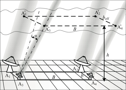
Figure 1.— Schematic of the CARMA Paired Antenna Calibration System. Antennas $A_{1}$ and $A_{2}$ (in the science array) observe the science target while antennas $A_{3}$ and $A_{4}$ (in the reference array), offset by a distance $b$ from the science array, observe a bright atmospheric calibrator. In the turbulent layer at an elevation $h$ the beams are separated by a distance $b_{\mathrm{eff}}$ that depends on $b$, $h$, and the angular offset between the science and reference sources, $\alpha$. If the effective baseline, $b_{\mathrm{eff}}$, is much smaller than the science baseline, $B$, the delay difference to the reference antennas is a good estimate for the delay difference to the science antennas.

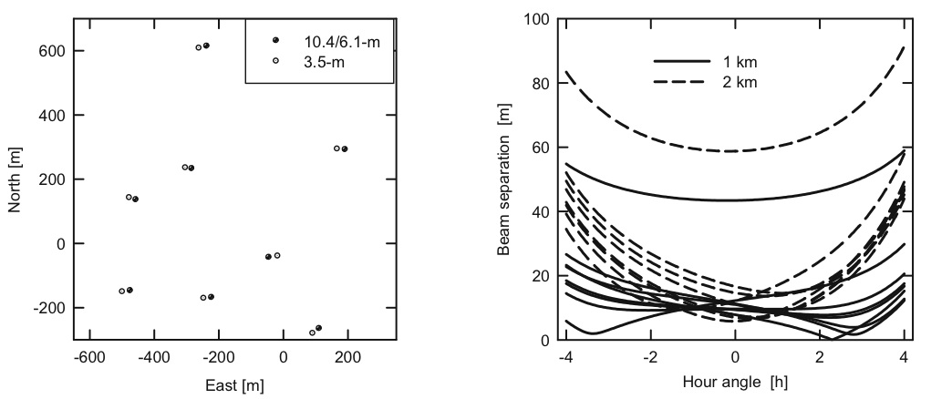
Figure 2.— The left panel shows the locations of the science (10.1-m and 6.4-m) and reference (3.5-m) antennas in the B-configuration of CARMA (circles do not represent the actual antenna diameters). The right panel shows the separation, $b_{\mathrm{eff}}$, between the science and reference beams in the turbulent layer for each pair of antennas during the PP 13S* observations. The continuous (dashed) line corresponds to a turbulent layer at a 1(2)-km altitude. For most pairs the configuration is very favorable, giving rise to effective baselines much shorter than the science baseline.

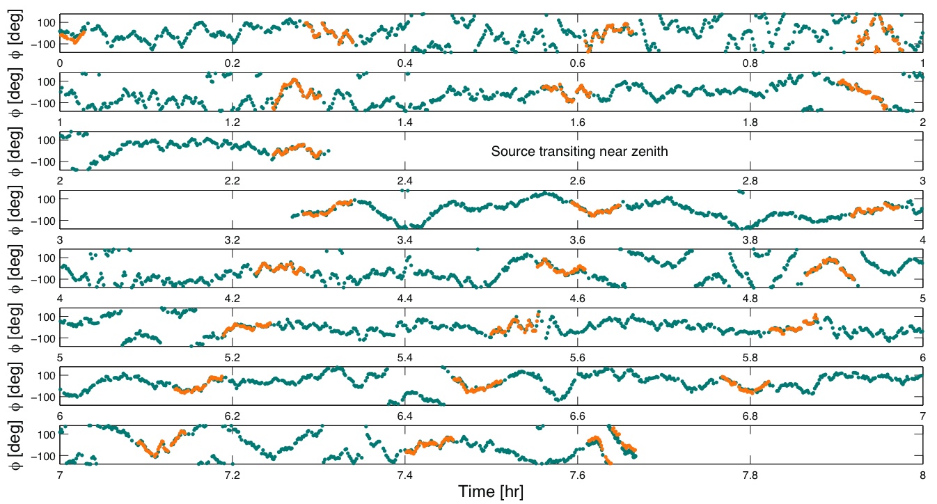
Figure 3.— Visibility phase versus time for the science array (orange) and the reference array (green) measured toward 3C111 on a baseline of length $\sim 800$ m in B configuration. The phase measured by the reference array at a frequency of 30.4 GHz was scaled to the frequency of the science array (227 GHz) by a factor of 7.5 (= 227 GHz / 30.4 GHz). Each data point indicates the measured phase over a 4 s integration after removing the mean phase computed in 10 min intervals. About 1 h of data are omitted near the middle of the observation when PP 13S* and 3C111 were transiting at an elevation $>80\arcdeg$ and the tracking of the antennas was poor. The figure demonstrates that the observed phases at 30.4 GHz closely track the phases measured at 227 GHz and can be used to correct the atmospheric fluctuations at higher frequencies.

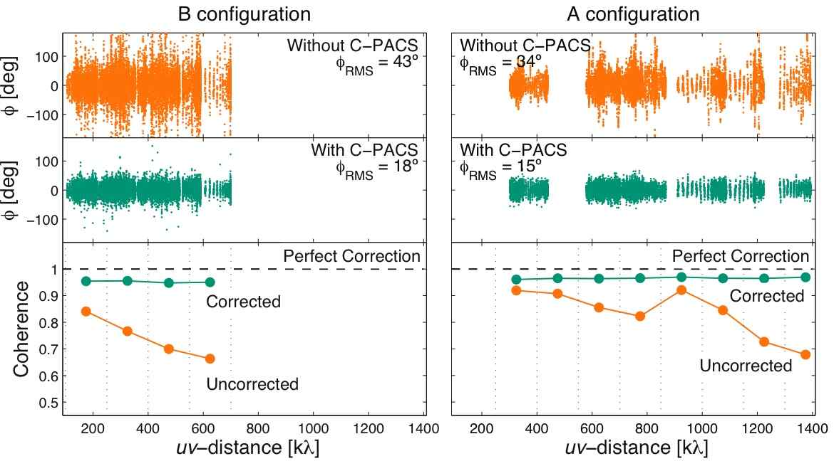
Figure 4.— Visibility phases versus $uv$-distance on all paired baselines for observations of 3C111 in the CARMA B and A configurations. The phases are shown before (top panels) and after (middle panels) applying C-PACS corrections. Each point indicates the measured phase in a 4 s integration after removing the mean phase computed in 10 min intervals. The bottom panels show the coherence calculated over 130 k$\lambda$ intervals. Before applying C-PACS, the coherence declines with $uv$-distance as expected for atmospheric phase fluctuations that increase with baseline length. After applying C-PACS, the phase coherence is higher and uniform with baseline length.

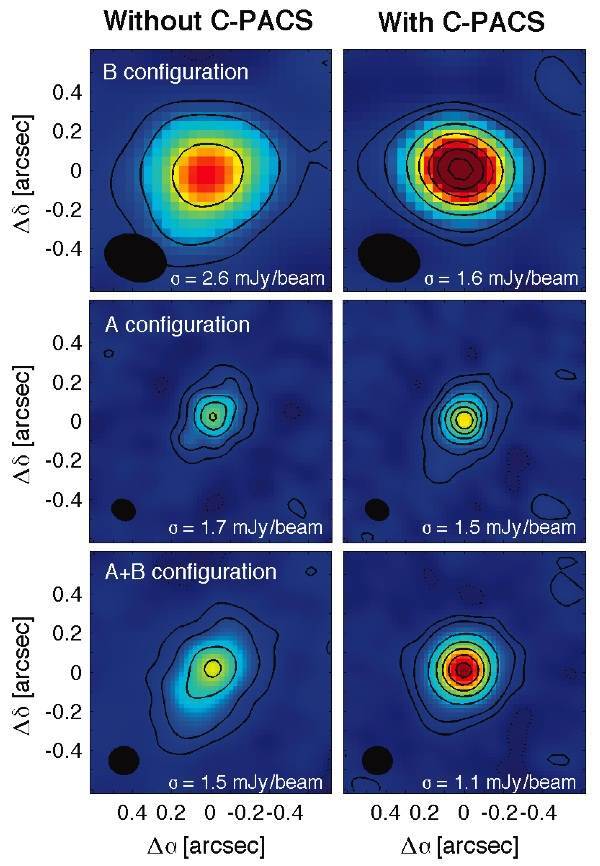
Figure 5.— CARMA 227 GHz continuum images of PP 13S* before (left) and after (right) C-PACS corrections for data obtained in B configuration (top), A configuration (middle), and B and A configurations combined (bottom). No absolute flux scale or amplitude gain calibration have been applied to the data in order to assess the effect of atmospheric phase corrections only. The color scale range is same for all maps (from -2.4 to 54.8 mJy) such that the measured fluxes can be compared directly. Solid contours are at 2$\sigma$, $5\sigma$ and in increments of 5$\sigma$ thereafter. Dotted contour is at $-2\sigma$. For both B and A configurations, applying the C-PACS correction increased the observed peak flux and reduced the observed source size.

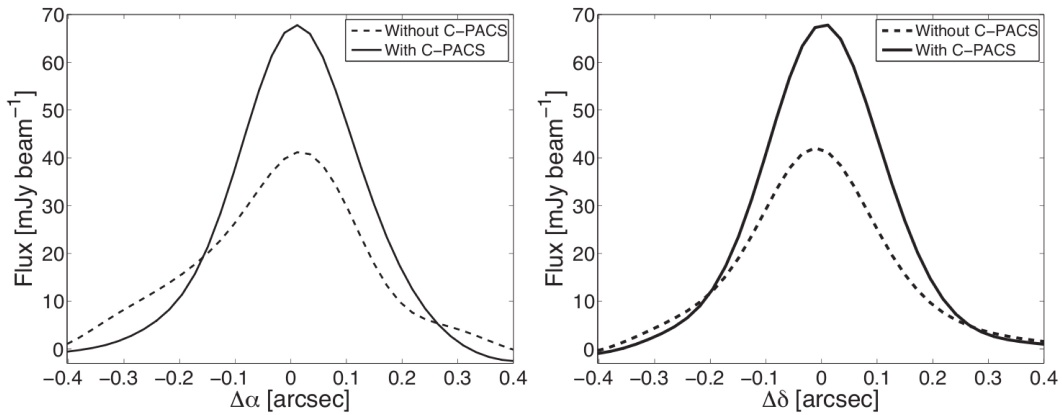
Figure 6.— Observed flux density toward PP 13S* versus offset in right ascension (left) and declination (right) before and after applying C-PACS corrections. Applying C-PACS corrections increased the peak flux density and decrease the observed source size.

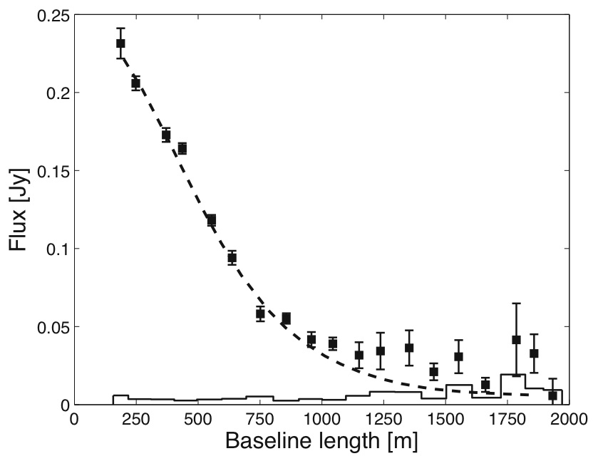
Figure 7.— Observed visibility amplitudes toward PP 13S* after applying the C-PACS corrections (black points) versus the deprojected baseline length. The errorbars indicate the 1$\sigma$ interval uncertainties, but exclude uncertainties in the flux calibration ($\sim$ 20%). The histogram shows the expected signal for random noise. The dashed line shows the best-fit disk model (see text) to the visibility data. The clear decline in the visibility amplitude with baseline length indicates the dust emission around PP 13S* has been resolved.

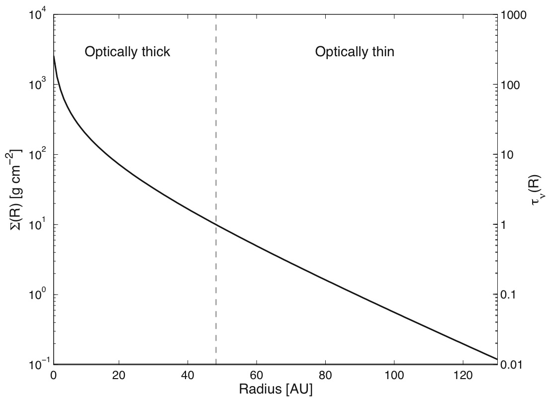
Figure 8.— Model surface density distribution of PP 13S* as a function of disk radius. The disk optical depth ($\tau=\Sigma_{d}(R)\times\kappa_{1.3mm}$) was computed assuming a constant dust opacity throughout the disk. The inner region of the disk ($R<48$ AU) becomes optically thick at a frequency of 227 GHz.

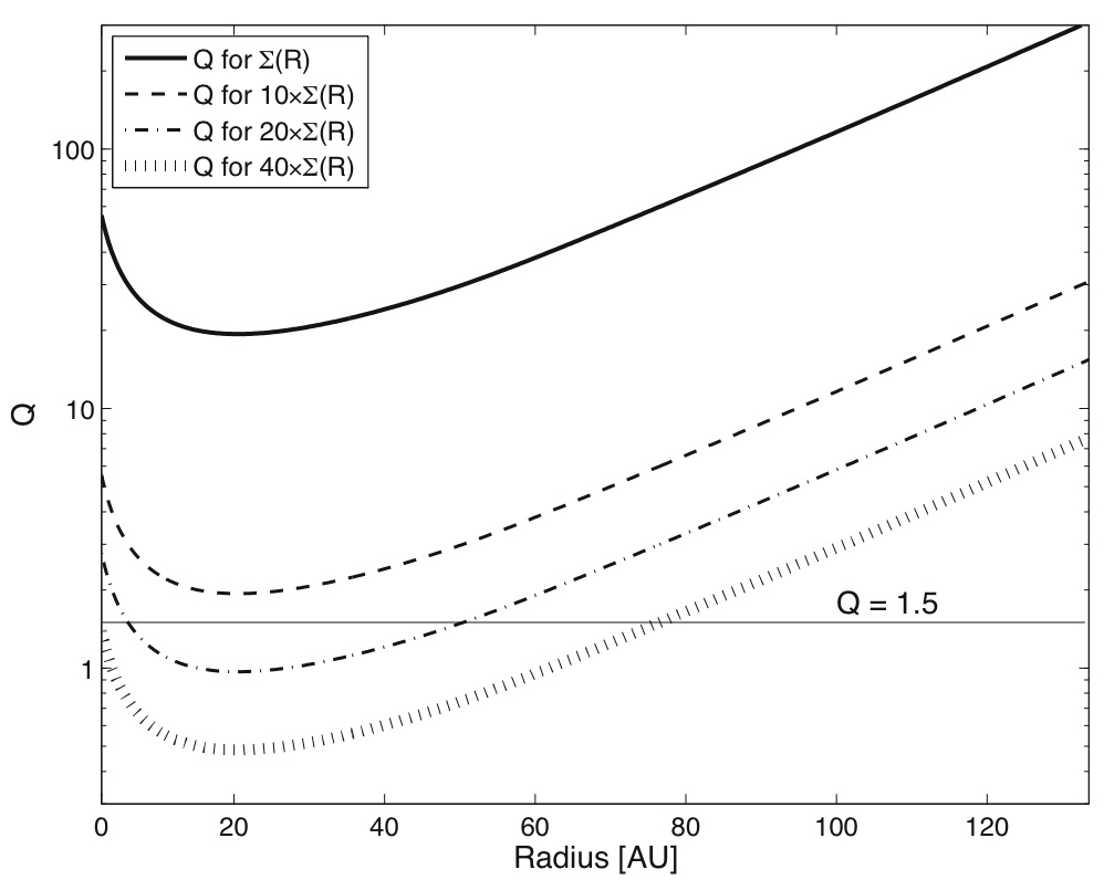
Figure 9.— Toomre’s instability parameter, $Q$, plotted for the PP 13S* disk. The solid line shows the $Q$ values for the nominal disk model. Dust opacities that are 10, 20 and 40 times larger than the adopted opacities are shown by the dashed, dash-dotted, and vertical-dashed curves respectively. The $Q=1.5$ limit is shown for reference, such that regions with $Q\lesssim 1.5$ may become gravitational unstable. The disk surface density needs to be an order of magnitude higher than the nominal model in order to form instabilities in the disk.

References

- Andrews & Williams (2005) Andrews, S. M., & Williams, J. P. 2005, ApJ, 631, 1134
- Andrews & Williams (2007a) Andrews, S. M., & Williams, J. P. 2007a, ApJ, 671, 1800
- Andrews & Williams (2007b) Andrews, S. M., & Williams, J. P. 2007b, ApJ, 659, 705
- Armitage et al. (2001) Armitage, P. J., Livio, M., & Pringle, J. E. 2001, MNRAS, 324, 705
- Asaki et al. (1996) Asaki, Y., Saito, M., Kawabe, R., Morita, K.-I., & Sasao, T. 1996, Radio Science, 31, 1615
- Asaki et al. (1998) Asaki, Y., Shibata, K. M., Kawabe, R., Roh, D.-G., Saito, M., Morita, K.-I., & Sasao, T. 1998, Radio Science, 33, 1297
- Aspin & Reipurth (2000) Aspin, C., & Reipurth, B. 2000, MNRAS, 311, 522
- Aspin & Sandell (2001) Aspin, C., & Sandell, G. 2001, MNRAS, 328, 751
- Clark (1980) Clark, B.G. 1980, A&A, 89, 377
- Cohen et al. (1983) Cohen, M., Aitken, D. K., Roche, P. F., & Williams, P. M. 1983, ApJ, 273, 624
- Condon & Yin (2001) Condon, J. J., & Yin, Q. F. 2001, PASP, 113, 362
- Hales et al. (2003) Hales, S, Hills, R., Robson, Y., Richer, J., Delgado, G., Otrola, A., Radford, S. 2003, ALMA Memo 459
- Hartmann & Kenyon (1996) Hartmann, L., & Kenyon, S. J. 1996, ARA&A, 34, 207
- Hill (1988) Hill, R. J. 1988, IEEE Transactions on Antennas and Propagation, 36, 423
- Högbom (1974) Högbom, J. A. 1974, A&AS, 15, 417
- Holdaway et al. (1995) Holdaway, M.A., Radford, S. J. E., Owen, F. N., Foster, S. M. 1995, MMA Memo 139
- Isella et al. (2009) Isella, A., Carpenter, J. M., & Sargent, A. I. 2009, ApJ, 701, 260
- Kolmogorov (1941) Kolmogorov, A. 1941, Akademiia Nauk SSSR Doklady, 30, 301
- Jennison (1958) Jennison, R. C. 1958, MNRAS, 118, 276
- Kwon et al. (2009) Kwon, W., Looney, L. W., Mundy, L. G., Chiang, H.-F., & Kemball, A. J. 2009, ApJ, 696, 841
- Lay (1997) Lay, O. P. 1997, A&AS, 122, 535
- Lay (1997b) Lay, O. P. 1997b, A&AS, 122, 547
- Lodato & Rice (2004) Lodato, G., & Rice, W. K. M. 2004, MNRAS, 351, 630
- Parsamian & Petrossian (1979) Parsamian, E. S., & Petrossian, V. M. 1979, Soobshcheniya Byurakanskoj Observatorii Akademiya Nauk Armyanskoj SSR Erevan, 51, 12
- Pollack et al. (1994) Pollack, J. B., Hollenbach, D., Beckwith, S., Simonelli, D. P., Roush, T., & Fong, W. 1994, ApJ, 421, 615
- Sandell & Aspin (1998) Sandell, G., & Aspin, C. 1998, A&A, 333, 1016
- Sandell & Weintraub (2001) Sandell, G., & Weintraub, D. A. 2001, ApJS, 134, 115
- Sault et al. (1995) Sault, R. J., Teuben, P. J., & Wright, M. C. H. 1995, Astronomical Data Analysis Software and Systems IV (ASP Conf. Ser. 77), ed. R. A. Shaw, H. E. Payne, & J. J. E. Hayes (San Francisco, CA: ASP), 433
- Schwab (1980) Schwab, F. R. 1980, Proc. SPIE, 231, 18
- Smith (1993) Smith, R. G. 1993, MNRAS, 264, 587
- Sramek (1983) Sramek, R. A. 1983, VLA Test Memo, No. 143
- Sramek (1989) Sramek, R. A. 1989, VLA Test Memo, No. 175
- Steer, Dewdney, & Ito (1984) Steer, D. G., Dewdney, P. E., & Ito, M. R. 1984, A&A, 137,159
- Stirling et al. (2006) Stirling, A., Richer, J., Hills, R., & Pardo, J. 2006, Proc. SPIE, 6267, 63
- Tatarskii (1961) Tatarskii, V. I. 1961, Wave Propagation in a Turbulent Medium (New York:Dover)
- Thompson et al. (2001) Thompson, A. R., Moran, J. M., & Swenson, G. W. Jr. 2001, Interferometry and Synthesis in Radio Astronomy, 2nd ed. (New York: Wiley-Interscience)
- Westwater (1967) Westwater, E. R. 1967, ESSA Technical Report IER 30-ITSA 30
- Woody et al. (2000) Woody, D. J., Carpenter, J., & Scoville, N. 2000, in ASP Conf. Ser. 217, Imaging at Radio Through Submillimeter Wavelengths, ed. J. G. Mangum & S. J. E. Radford (San Francisco: ASP), 31
- Wright et al. (2009) Wright, E. L., et al. 2009, ApJS, 180, 283