Abstract

In 2008 the CDF collaboration discovered a large excess of events containing two or more muons, at least one of which seemed to have been produced outside the beam pipe. We investigate whether similar “ghost” events could (and should) have been seen in already completed experiments. The CDF di–muon data can be reproduced by a simple model where a relatively light $X$ particle undergoes four–body decay. This model predicts a large number of ghost events in Fermilab fixed–target experiments E772, E789 and E866, applying the cuts optimized for analyses of Drell–Yan events. A correct description of events with more than two muons requires a more complicated model, where two $X$ particles are produced from a very broad resonance $Y$. This model can be tested in fixed–target experiments only if the cut on the angles, or rapidities, of the muons can be relaxed. Either way, the UA1 experiment at the CERN $p\bar{p}$ collider should have observed ${\cal O}(100)$ ghost events.

1 Introduction

In 2008 the CDF Collaboration published an analysis of events containing at least two muons, and found a large excess of so–called ghost events, which supposedly cannot be explained by the known QCD production with the current understanding of the CDF detector [1]. The two muons with the highest transverse momenta in a sample event, the so-called initial muons, each were required to have transverse momentum $p_{T}\geq 3\,\mathrm{GeV}$, a pseudorapidity $|\eta|\leq 0.7$ and a combined invariant mass in the range $5\,\mathrm{GeV}<m_{\mu\mu}\leq 80\,\mathrm{GeV}$. In the following these cuts are called two–muon cuts.

In defining these muon tracks, no information from the silicon microvertex detector (SVX) is used. According to CDF, some 24 % of muon pairs passing the above cuts should have been detected by the SVX if they come from known sources. These are called QCD background events by CDF, and chiefly originate from Drell–Yan pairs, semileptonic decays of $c$ and $b$ quarks, and misidentified charged hadrons. However, only in about 19 % of the observed di–muon events both muons were also detected by the SVX. CDF therefore concludes that there is a large number of ghost events where at least one initial muon is produced outside of the beam pipe (more exactly, outside the first layer of the SVX, which is adjacent to the beam pipe) with a radius of $15\,\mathrm{mm}$. Indeed, many of the primary muons were found to have a large impact parameter.

Moreover, nearly 10 % of these events contained one or several additional muons with $p_{T}\geq 2\,\mathrm{GeV}$ and $|\eta|\leq 1.1$, many of which again have a high impact parameter; this fraction is about four times higher than one expects for QCD events. Furthermore, the ghost sample contains approximately equally many same–sign (SS) and opposite–sign (OS) initial muon pairs.

After correcting for events from ordinary sources, i.e. QCD production, CDF finds $84895\pm 4829$ ghost events within a data sample corresponding to an integrated luminosity of $742\,\mathrm{pb^{-1}}$. The ghost cross section

$$\sigma(p\bar{p}\rightarrow{\rm ghosts})=\frac{84895\pm 4829}{742}\,\mathrm{pb}\approx(114.4\pm 6.5)\,\mathrm{pb}$$

is comparable in size to the $b\bar{b}$ contribution to the di–muon sample:

$$\sigma(p\bar{p}\rightarrow b\bar{b}\rightarrow\mu\mu)=\frac{221564\pm 11615}{742}\,\mathrm{pb}\approx(298.6\pm 15.7)\,\mathrm{pb}.$$

Considering this high cross section and the remarkable properties of the ghost events it is natural to ask whether such events could (and hence presumably should) have been observed in earlier experiments. This question can be answered only in the framework of concrete particle physics models. In the following Section we therefore first describe properties of the ghost particles (whose decays produce the detected muons) that can be derived almost model–independently from the CDF data. In Sec. 3 we describe a simple model that reproduces most of the features of most ghost events [1]. This model indeed predicts that experiments at lower energies should have observed dozens to thousands of ghost events. We then construct a somewhat more complicated model, which improves the description of the subset of ghost events containing at least three muons; this model is much more difficult to probe at fixed–target experiments. Finally, we conclude.

2 General Considerations

As described above, muons in ghost events seem to originate at a large distance from the primary interaction vertex. This indicates that the muons are produced in the decays of rather long–lived $X$ particles.

Many properties of the $X$ particle follow from the properties of the ghost events. First, the $X$ particles should be electrically neutral. Otherwise they would have escaped detection by LEP experiments only if their mass exceeded 100 GeV, which would have put their cross section closer to that for $t\bar{t}$ production than that for $b\bar{b}$ production. Moreover, the $X$ particles themselves would then have produced a track which in many cases should have been easier to detect by the SVX than a muon track, since such heavy $X$ particles would often have had smaller velocity, and hence larger energy loss $dE/dx$, than ultra–relativistic muons.

The $X$ particles should have an average decay length $\gamma\tau_{X}v\geq 15\,\mathrm{mm}$, in order to account for the high impact parameters of the ghost muons and in particular for the fact that at least one initial muon appears to be created outside of the beam pipe. On the other hand, the decay length cannot be very much larger than 15 mm, since both muons originate well within the CDF tracker.

The fact that approximately equally many SS and OS ghost di–muon events are observed indicates that the $X$ particle should be a Majorana particle, i.e. identical to its CP conjugate.

Finally, the fact that a significant fraction of ghost di–muon events contains additional “secondary” muon indicates that all $X$ particles decay into a final state with relatively high multiplicity. Otherwise the branching ratio into multiple muons would be expected to be very small. On the other hand, the higher the decay multiplicity, the more complicated a full (renormalizable) quantum field theory reproducing our phenomenological model would have to be. In our simulations we therefore assume that all $X$ particles decay into four elementary fermions, at least one of which is a muon. We model these decays using pure phase space, i.e. assuming constant decay matrix elements.

3 Simple Model

In order to proceed further, we have to make assumptions regarding the production mechanism of $X$ pairs. In our simple model we assume that the $X$ particles are pair–produced directly in either gluon–gluon fusion or quark–antiquark annihilation, with differential $S-$wave cross section

$$\frac{d\sigma(gg/q\bar{q}\rightarrow XX)}{d\cos\theta}=N_{gg/q\bar{q}}\cdot\frac{\beta}{\hat{s}}=N_{gg/q\bar{q}}\cdot\frac{\sqrt{1-\frac{4m^{2}_{X}}{\hat{s}}}}{\hat{s}}.$$ (3.1)

Here $\hat{s}$ is the squared partonic center of mass energy, $m_{X}$ is the mass of the $X$ particle, $\beta$ is the velocity of the $X$ particles in the partonic center of mass frame, and $N_{gg/q\bar{q}}$ are constants which are fixed by the requirement that we reproduce the ghost cross section measured by CDF.

We want to use the simple model to estimate the number of ghost di–muon events that should have been detected by earlier experiments operating at lower center of mass energies. Using the fact that about half of these events contain like–sign muons, as well as the large impact parameters of these muons, should suppress physics backgrounds to negligible levels. Possible instrumental backgrounds can only be evaluated by the experiments themselves.

The free parameters of this simple model are the decay modes and corresponding branching ratios of the $X$ particle, its mass and lifetime. We set the lifetime as

$$c\tau_{X}=20\,\mathrm{mm}\,;$$ (3.2)

this choice only affects the impact parameter distribution of the ghost muons, but no other results.

We include the following decay modes:

• 1–muon: $X\rightarrow\mu^{-}\bar{\nu}_{\mu}u\bar{d}$  or  $X\rightarrow\mu^{+}\nu_{\mu}\bar{u}d$

• 2–muon: $X\rightarrow\mu^{-}\mu^{+}u\bar{u}$  or  $X\rightarrow\mu^{-}\mu^{+}d\bar{d}$

• 4–muon: $X\rightarrow\mu^{-}\mu^{+}\mu^{-}\mu^{+}$

Our assumption the $X$ is a Majorana particle implies that charge conjugate modes contribute with equal branching ratio. These decays conserve electric charge and all lepton numbers. Spin conservation then implies that $X$ is a boson.

In order to simulate $p\bar{p}\rightarrow XX\rightarrow\mu^{+}\mu^{-}+\dots$ events, we implemented the production cross sections (3.1) into HERWIG++ [2], using default parameters for parton showering and the underlying event. Recall that we model $X$ decays assuming constant decay matrix elements.

Fig. 5 in Ref. [1] shows that the di–muon excess occurs at rather small invariant mass of the primary muon pair, $m_{\mu\mu}\raisebox{-3.69899pt}{~{}\shortstack{$<$ \\ [-0.07cm] $\sim$}}~{}40\,\mathrm{GeV}$. Together with the large cross section for ghost events this argues for a relatively light $X$ particle. Unfortunately no $p_{T}$ spectrum of the primary muons in ghost events is provided, which might have allowed to estimate $m_{X}$ from the bulk of events that do not contain additional muons.

We therefore use the invariant mass distribution of all muons contained in the 27,990 $36.8^{\circ}$ cones (corresponding to $\cos\theta=0.8$) around initial muons which contain at least one additional muon (see Fig. 34a in [1]). This distribution matches the invariant mass distribution in each cone for the events, in which both cones contain at least one additional muon (Fig. 34b in [1]). This agrees with our model, in which both $X$ particles contribute one initial muon each with identical cone properties. In most cases only additional muons from the decay of the same $X$ particle that produced the initial muon are contained in the $36.8^{\circ}$ cone around the initial muon. The reason is that in the partonic center of mass system the $X$ particles propagate in opposite directions. The measured invariant mass distribution of all muons in these cones is shown in the left frame of Fig. 1; it peaks around $0.6\,\mathrm{GeV}$, and becomes very small beyond $3\,\mathrm{GeV}$. Our best fit value for the mass of the $X$ particle is

$$m_{X}=1.8\,\mathrm{GeV}.$$ (3.3)

The corresponding distribution is shown in the right frame of Fig. 1, ignoring measurement errors and assuming $X$ pair production from $q\bar{q}$ annihilation. We consider the agreement satisfactory.

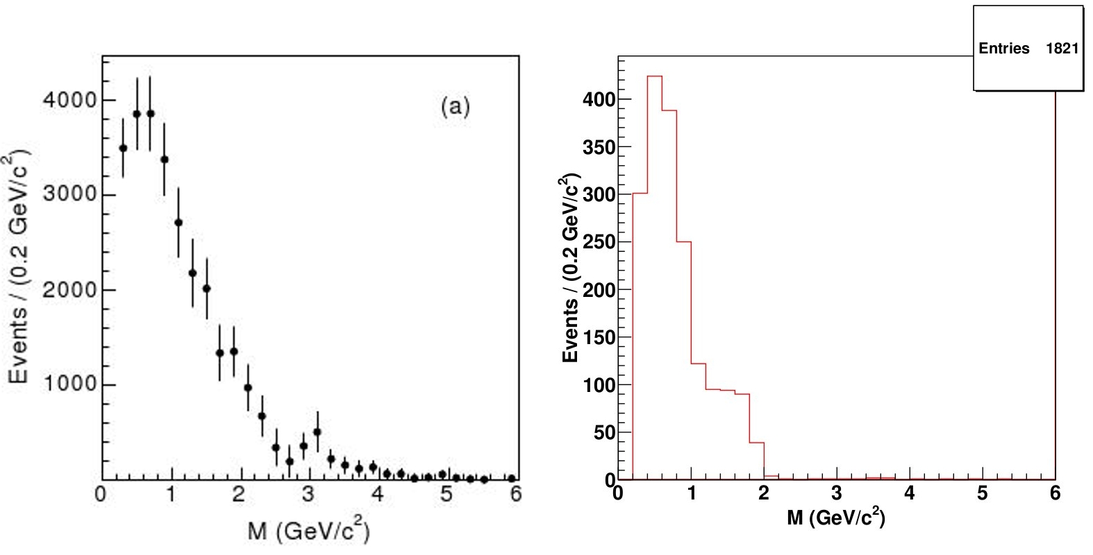
Figure 1: Invariant mass distribution of all muons within $36.8^{\circ}$ cones around initial muons which contain at least one additional muon, for the ghost measurement (left) [Fig. 34a in [1]] and our simulation (right). The simple model parameters for the process $q\bar{q}\rightarrow XX$ are used in the simulation. 21,745 of 40 million simulated events pass the two–muon cuts.

Finally, we determine the branching ratios for the various $X$ decay modes by using the sign–coded muon multiplicity distribution of additional muons found in $36.8^{\circ}$ cones around the initial muons. Here each additional muon with the same charge as the primary muon increases the count by ten, whereas each additional muon with the opposite charge as the primary muon counts as one. In case of $X$ pair production from quark–antiquark annihilation our fit for the branching ratios is 93.88 % for the 1–muon, 5.02 % for the 2–muon, and 1.10 % for the 4–muon decay. The gluon fusion mechanism requires slightly different branching ratios, because of the different efficiencies for the generated muons to pass the cuts.

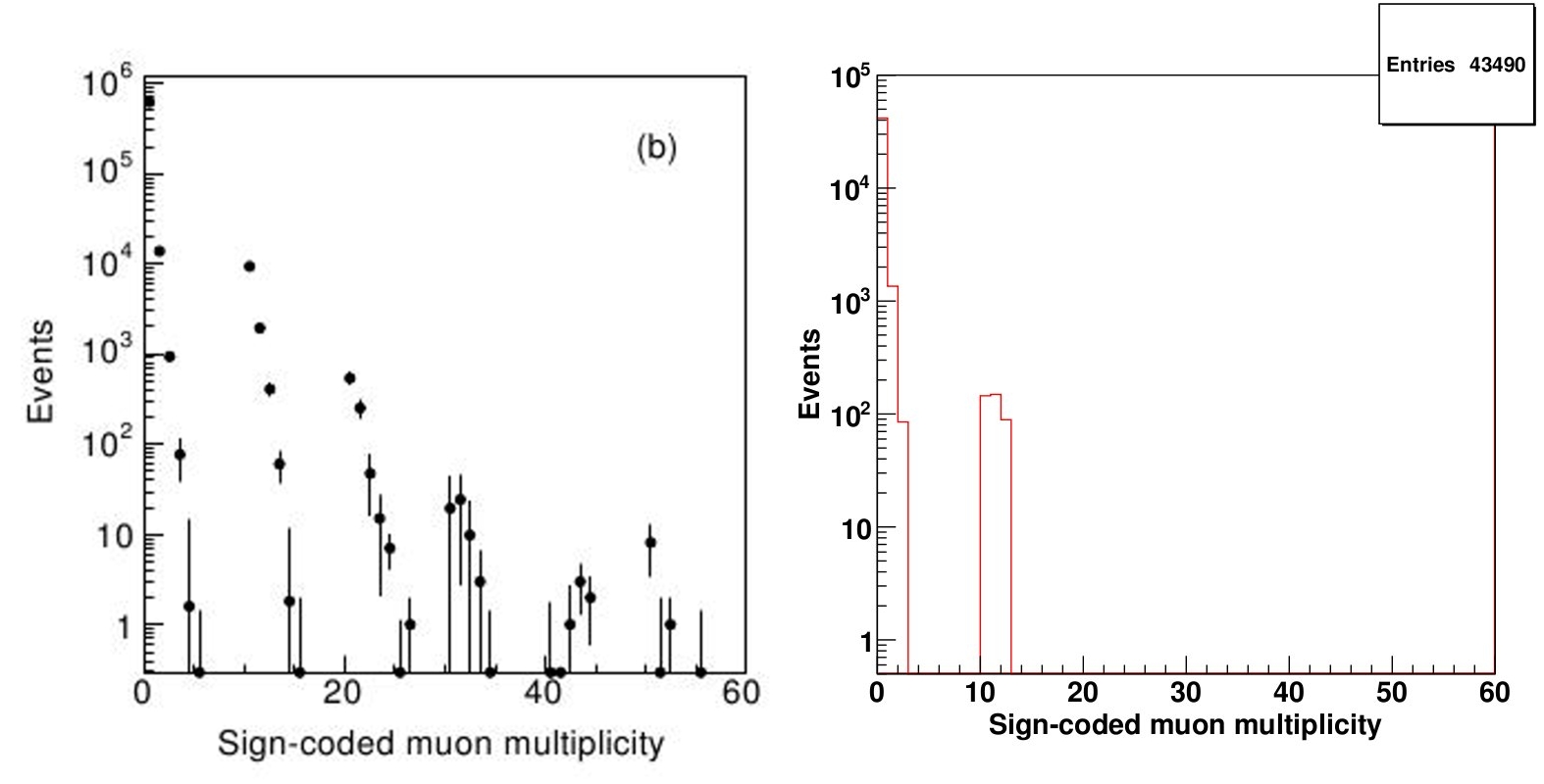
Figure 2: Sign-coded muon multiplicity distribution of additional muons found in $36.8^{\circ}$ cones around initial muons for the ghost measurement (left) [Fig. 22b in [1]] and our simulation (right). The simple model parameters for the process $q\bar{q}\rightarrow XX$ are used in the simulation. 21,745 of 40 million simulated events pass the two–muon cuts.

Fig. 2 compares the original CDF result (Fig. 22b in [1]) with our simulation. Clearly our model produces fewer entries at high muon multiplicities. Furthermore, the ratio between cones with one OS additional muon, i.e. the number of entries in “1”, and with one SS additional muon, i.e. the number of entries in “10”, is too high. The higher number of entries in “1” follows from the construction of the decay modes. Since all muons inside a cone usually result from the decay of the same $X$ particle, the 2–muon decay only contributes to “1” and the 4–muon decay gives two times more entries in “1” than in “10”. In order to reproduce this ratio correctly, we need a 2–muon decay with SS muons. The conservation of electric charge, all single lepton numbers and spin then requires a decay into at least eight elementary fermions, e.g. $X\rightarrow\mu^{+}\mu^{+}\nu_{\mu}\nu_{\mu}\bar{u}d\bar{u}d$. One would obviously need a very contrived model to reproduce this in a renormalizable quantum field theory. Another possibility is to allow violation of separate lepton numbers, insisting only that the total lepton number remains conserved; we will pursue this in our more complicated model.

Furthermore, our simple model almost never generates events with more than three additional muons in a $36.8^{\circ}$ cone around a primary muon. This discrepancy with the data may be considered less problematic, since it concerns only a small fraction of all ghost events. In addition these multi–muon events are presumably more prone to experimental errors. For example, an underestimated fake muon rate would affect the extracted rate of events with multiple muons more than that of events with fewer muons; note that the fake muon contribution has been subtracted by CDF in the result reproduced in the left frame of Fig. 2.

We emphasize that we want to use our model only to estimate di–muon rates. While the multi–muon events are indeed spectacular, they have substantially reduced cross sections. Recall also that there is very little physics background to di–muon events where the muons originate a few cm from the primary interaction vertex.

Having fixed the parameters of the model, we are ready to make predictions for the number of expected ghost events in various experiments. We focus on experiments that had the possibility to identify muons, and accumulated large data samples. These include the experiment UA1 at the CERN $p\bar{p}$ collider [3], and the Fermilab fixed–target experiments E605 [4], E772 [5], E789 [6] and E866 [7]. E789 is especially interesting for our purposes since it featured a vertex detector, which should have had no trouble detecting the long flight path of $X$ particles if some of them had been produced. We also considered the HERA experiments ZEUS and H1, where $X$ pairs could have been produced in “resolved” photoproduction processes involving the parton distribution functions inside the photon; however, we found that they are not sensitive to our model, since the cross section is suppressed by a factor $\alpha_{\rm em}^{2}$ and the integrated luminosity is not very high.

Table 1 shows the cuts which we use for the simulations. Since we focus on di–muon events, we only cut on the momenta of these muons. In case of the UA1 experiment, the cuts can be taken directly from their analyses of di–muon data [3]. The fixed–target experiments are more difficult to simulate, since not enough information is provided in their analyses of di–muon data to completely determine their acceptance region. It should be noted that these analyses were optimized for Drell–Yan muon pairs, which to leading order emerge back–to–back in the partonic center of mass system. This is usually not the case for the muon pairs from $X$ decays.

Table 1: Cuts on the two muons in the experiments we consider. Except for E789 all cuts are applied in the hadronic center of mass system. The cuts for E789 are applied in the lab frame.

Exp.	$\sqrt{s}$ [GeV]	$p_{T,\,{\rm min}}$ [GeV]	Inv. mass [GeV]	Pseudorapidity
CDF	1960	3	$5<m_{\mu\mu}\leq 80$	$|\eta|\leq 0.7$
UA1–a	546	3	$6<m_{\mu\mu}$	$|\eta|\leq 0.7$
UA1–b	630	3	$6<m_{\mu\mu}$	$|\eta|\leq 0.7$
UA1–c	630	3	$6<m_{\mu\mu}<35$	$|\eta|\leq 0.7$
E605–a	38.8	—	$7<m_{\mu\mu}<18$	$|\eta|\leq 0.02$
E605–b	38.8	—	$6<m_{\mu\mu}<18$	$|\eta|\leq 0.02$
E772–a	38.8	—	$4.5\leq m_{\mu\mu}\leq 9$ or $11\leq m_{\mu\mu}$	$|\eta|\leq 0.044$
E772–b	38.8	—	$4\leq m_{\mu\mu}$	$|\eta|\leq 0.044$
E789	38.8	—	$2\leq m_{\mu\mu}\leq 6$	$3.506\leq\eta\leq 4.605$
E866	38.8	—	$4\leq m_{\mu\mu}\leq 9$ or $10.7\leq m_{\mu\mu}$	$|\eta|\leq 0.02$

In detail, the fixed–target experiments do not cut on $p_{T}$, since they are sensitive to muons even in the very forward direction. The lower bounds on the di–muon invariant mass $m_{\mu\mu}$ are determined from the acceptances of these experiments as described in their publications. The upper bounds on $m_{\mu\mu}$ are basically irrelevant given the small center of mass energy of these experiments. Finally, the (very stringent!) cut on the pseudorapidity $|\eta|$ results from the main focus on Drell–Yan events within these experiments. In the partonic center of mass system the angular dependence of a created Drell–Yan di–muon pair is given by $(1+\cos\theta_{cs})$. For E605 the acceptance of the muon–detectors is restricted to a “small range of the decay angle” near $\theta_{cs}=90^{\circ}$ [4]. Because this small range is not further specified, we use the acceptance plots in Figs. 8 and 9 in Ref. [4] to estimate a spatial coverage of around 2 %, i.e. $\theta_{cs}\in[-0.02,0.02]$. In the limit where the angular distributions of both muons are independent of each other, the acceptance decreases to $0.04\,\mathrm{\%}$, resulting in a much worse acceptance for ghost events than for Drell–Yan events. Moreover, in contrast to Drell–Yan events we cannot reconstruct the partonic center of mass system from the measured primary muons in ghost events. We therefore work within the hadronic center of mass system. The pseudorapidity cut $|\eta|\leq 0.02$ given in Table 1 then approximately reproduces the angular coverage given above.

Like E605 the fixed–target experiment E772 features a small spatial muon coverage which is not specified clearly [5]. Therefore we again have to estimate the pseudorapidity cut. We compared the data sets E605–a, E605–b and E772–a, taking into account their different di–muon invariant mass acceptances and integrated luminosities. Using the given differential Drell–Yan cross section $m^{3}_{\mu^{+}\mu^{-}}d^{2}\sigma^{DY}/dm_{\mu^{+}\mu^{-}}dx_{F}$ for fixed Feynman$-x$ we can determine the invariant mass dependence of the total cross section; see Fig. 3 in the first and Table 1 in the second publication of Ref. [5]. We find $\sigma^{DY}\propto m^{-5}_{\mu^{+}\mu^{-}}$, where $m_{\mu^{+}\mu^{-}}$ is the lower mass limit. Starting from the 2 % acceptance of E605 we estimate the cut $|\eta|\leq 0.044$ for E772; see Table 1.

We use the pseudorapidity cut $|\eta|\leq 0.02$ for the fixed–target experiment E866, because no further information on the muon acceptance is provided in Ref. [7]. Note that the detectors of all the Fermilab fixed–target experiments we consider are based on the original E605 detector. The experiment E789 provides explicit pseudorapidity coverage information within the lab frame [6].

The CDF efficiency for identifying a muon pair is approximately $26\,\mathrm{\%}$ [1]. We adopt this efficiency for the UA1 experiment as well. The fixed–target experiments have efficiencies of the order of $90\,\mathrm{\%}$ after cuts.

Our results are shown in Table 2. The errors of the predictions result from the errors of the CDF measurement, of the simulated cross sections, of the integrated luminosities, of the efficiencies for the di–muon acquisition and of the efficiency for the simulated events to pass the di–muon cuts. The last of these errors dominates for most of the fixed–target experiments. Since the acceptance is very small, it is difficult to accumulate sufficient statistics. We tried to overcome this problem by relaxing the upper limit $\eta_{\rm max}$ on the absolute value of the pseudorapidity in the hadronic center of mass frame, taking different values for this cut. We then fit the resulting efficiency to a quadratic function of $\eta_{\rm max}$, which we finally extrapolate to the value of $\eta_{\rm max}$ given in Table 1.

Table 2: Expected number of ghost events for the simple model compared to the number of actually observed di–muon events. The fixed–target data sets only include OS di–muons. For E789 only the number of $J/\psi$ candidates is stated; the di–muon invariant mass distribution can be found in Fig. 1 in Ref. [6]. The normalization constants are $N_{gg}\approx(7.1\pm 0.4)\cdot 10^{-5}$ and $N_{q\bar{q}}\approx(1.8\pm 0.1)\cdot 10^{-3}$. The branching ratios for the gluon fusion mechanism are $93.32\,\mathrm{\%}$ for the 1–muon, $5.6\,\mathrm{\%}$ for the 2–muon and $1.08\,\mathrm{\%}$ for the 4–muon decay.

		# ghost events for		# of observed
Exp.	$\int{\cal L}dt$ [Nucl./pb]	$gg\rightarrow XX$	$q\bar{q}\rightarrow XX$	$\mu\mu$ events
CDF	$114.41\pm 6.51$	$84895\pm 4829$	$84895\pm 4829$	$84895\pm 4829$
UA1–a	0.108	$1.5\pm 0.1$	$5.6\pm 0.3$
UA1–b	0.6	$10.2\pm 0.6$	$33.9\pm 1.9$	880
UA1–c	4.7	$79.5\pm 4.5$	$261.5\pm 14.9$	2444
E605–a	$(1.14\pm 0.08)\cdot 10^{6}$	$30.4\pm 10.2$	$680.4\pm 325.6$	43663 (OS)
E605–b	$(2.7\pm 0.2)\cdot 10^{5}$	$2.0\pm 3.8$	$165.3\pm 151.2$	19470 (OS)
E772–a	$(5.8\pm 0.3)\cdot 10^{4}$	$39.9\pm 2.3$	$885.5\pm 68.9$	83080 (OS)
E772–b	$3.5\cdot 10^{5}$	$251.7\pm 28.8$	$9415.1\pm 547.1$	$\approx 450000$ (OS)
E789	$17.52\pm 1.89$	$134.7\pm 16.5$	$1294.9\pm 158.7$	$71206\pm 287$ ($J/\psi$)
E866	$3.78\cdot 10^{5}$	$144.4\pm 39.7$	$2339.2\pm 135.9$	$\approx 360000$ (OS)

We see that UA1 should have recorded about 100 (300) ghost di–muon pairs if $X$ pairs are produced predominantly from gluon fusion ($q\bar{q}$ annihilation). Recall that the cross section is normalized to the CDF data. Since the gluon distribution function inside the proton is softer than that of valence quarks, the cross section from gluon fusion decreases faster with decreasing $\sqrt{s}$ than that from $q\bar{q}$ annihilation. Note that UA1 did record about 3,300 di–muon events with the cuts listed in Table 1; about one quarter of these events contained a same–sign muon pair [3]. The UA1 data are compatible with SM predictions, with the biggest single contribution coming from $b\bar{b}$ production. It is not clear to us whether the UA1 detector would have been able to detect the rather long flight paths of the $X$ particles.

In case of the fixed–target experiments, we list the effective luminosity for nucleon–nucleon collisions. Here the predicted number of ghost events differs by about a factor of twenty between the two production mechanisms, with gluon fusion again leading to fewer events. However, even in that case we expect more than 100 events each in experiments E772, E789 and E866. This is far smaller than the total di–muon samples of these experiments. Recall, however, that in half of the ghost events both muons have the same charge. Moreover, the vertex detector of E789 should have been able to detect the displaced vertices from the $X$ decay. Although these experiments did not (yet) perform dedicated searches for ghost events, it seems unlikely that they would have escaped detection within the samples of Drell–Yan events.

4 More Complicated Models

4.1 Breit-Wigner Resonance

When fitting the parameters of the simple model discussed in the previous Section, we only compared to distributions of muons within a $36.8^{\circ}$ cone around the primary muons; see Figs. 1 and 2. In Fig. 3 we instead show the total invariant mass distribution of all muons in the small subsample of events in which the cones around both primary muons contain each at least one additional muon (Fig. 35a in [1]); these events thus contain a total of at least four muons. We see that our simple model predicts this distribution to peak slightly too early, and to fall off towards higher invariant masses much faster than the CDF data do. Recall that the invariant mass distribution of muons within each cone forced us to chose a rather small mass for the $X$ particle. We can thus only increase the number of events with large invariant mass of the multi–muon system by modifying the production cross section.

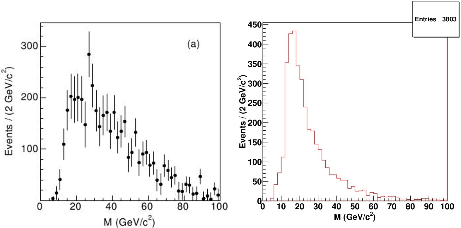
Figure 3: Invariant mass distribution of all muons within events in which both cones contain each at least one additional muon, for the ghost measurement (left) [Fig. 35a in [1]] and the simulation of our simple model (right). The process $q\bar{q}\rightarrow XX$ is simulated. In order to improve the efficiency, we forced both $X$ particles to decay into two muons; the small four muon channel does not change the result significantly. 20,212 out of 20 million generated events pass the cuts.

To this end, we introduce a Breit–Wigner (resonance) factor in the differential cross section:

$$\frac{d\sigma(gg/q\bar{q}\rightarrow Y\rightarrow XX)}{d\cos\theta}=N_{gg/q\bar{q}}^{BW}\cdot\frac{\hat{s}^{2}}{(\hat{s}-m_{Y}^{2})^{2}+\Gamma_{Y}^{2}m_{Y}^{2}}\cdot\frac{\sqrt{1-\frac{4m^{2}_{X}}{\hat{s}}}}{\hat{s}}$$ (4.1)

The constants $N_{gg/q\bar{q}}^{BW}$ are again chosen such that the total cross section measured by CDF is reproduced. $m_{Y}$ and $\Gamma_{Y}$ are the mass and width of the resonance. Fig. 4 shows that we can reproduce the data assuming $X$ pair production from quark–antiquark annihilation with $m_{Y}=\Gamma_{Y}=50\,\mathrm{GeV}$. Note that we can reproduce the slow fall–off towards high invariant masses only if the width has the same order of magnitude as the mass of the resonance, which implies that it is strongly coupled. The success of standard QCD in describing jet data at a variety of colliders suggests that the coupling of $Y$ to quarks or gluons is not very large. On the other hand, the coupling of $Y$ to $X$ is not constrained. In this scenario we expect most $Y$ “particles” to “decay” into $X$ pairs.

Figure 4: Invariant mass distribution of all muons within events in which both cones contain each at least one additional muon, simulated assuming $q\bar{q}\rightarrow Y\rightarrow XX$. The branching ratios are $93.43\,\mathrm{\%}$ for the 1–muon, $4.7\,\mathrm{\%}$ for the 2–muon and $1.87\,\mathrm{\%}$ for the 4–muon decay. 807,162 of 20 million generated events pass the two–muon cuts.

Since many $X$ particles are now produced with sizable transverse momentum, the efficiency for passing the di–muon cuts is larger than for the simple model. The muons produced in the two– and four–muon decay modes of $X$ are also somewhat more likely to pass the cut on additional muons. The branching ratios of $X$ therefore have to be chosen slightly differently from the simple model.

In this model we do not expect any ghost events in the fixed–target experiments we analyzed after the cuts of Table 1 have been imposed. This follows from two effects, which result from the higher center of mass energy of CDF ($1.96\,\mathrm{TeV}$) compared to the fixed–target experiments ($38.8\,\mathrm{GeV}$).

First, for given normalization, introducing the Breit–Wigner factor reduces the cross section. This reduction factor is much larger at the fixed–target experiments operating at $\sqrt{s}<m_{Y}$. For fixed ghost cross section at CDF, this reduces the fixed–target cross section before cuts by a factor of 64 (35) for the quark–antiquark annihilation (gluon fusion) mechanism.

Second, as mentioned above, introducing the Breit–Wigner factor increases the cut efficiency for the CDF experiment. This effect is much smaller for the fixed–target experiments, where the parton densities force most events to still have small partonic center of mass energy. Since we normalize to the CDF cross section after cuts, this reduces the event rate at the fixed–target experiments, e.g. for E789, by another factor of 16 for quark–antiquark annihilation and 41 for gluon fusion. In combination, these two effects reduce the expected event number for the fixed–target experiments by three orders of magnitude.

4.2 Muon Number Violating $X$ Decays

We saw in Sec. 3 that our simple model does not reproduce the sign–coded multiplicity distribution of additional muons very well. We argued that this is inevitable unless we allow $X$ decays into 8–body final states or allow violation of individual lepton numbers. Here we chose the second option, and consider the following $X$ decay modes:

• 1–muon: $X\rightarrow\mu^{-}\bar{\nu}_{\mu}u\bar{d}$   or  $X\rightarrow\mu^{+}\nu_{\mu}\bar{u}d$

• OS 2–muon: $X\rightarrow\mu^{-}\mu^{+}\tau^{-}\tau^{+}$

• SS 2–muon: $X\rightarrow\mu^{-}\mu^{-}\tau^{+}\tau^{+}$  or  $X\rightarrow\mu^{+}\mu^{+}\tau^{-}\tau^{-}$

• 4–muon: $X\rightarrow\mu^{-}\mu^{+}\mu^{-}\mu^{+}$

All these decays conserve total lepton number, but SS 2–muon decay violates $\tau$ and $\mu$ number separately (as do $\nu_{\mu}\leftrightarrow\nu_{\tau}$ oscillations). Note that we again use the simple $X$ pair production cross section without Breit–Wigner factor given in Eq. (3.1) in this Subsection. Fitting the $X$ mass and branching ratios to the in–cone multi–muon invariant mass and signed multiplicity distributions, respectively, we find $m_{X}=4.6\,\mathrm{GeV}$ and the branching ratios for the process $q\bar{q}\rightarrow XX$ are 82.32 % for the 1–muon, 5.99 % for the OS, 10.25 % for the SS 2–muon, and 1.44 % for the 4–muon decay. Note that some of the secondary muons now come from $\tau\rightarrow\mu$ decays, which produces rather soft muons. Moreover, the phase space available for the two direct muons in the $\mu\mu\tau\tau$ final states is quite small, i.e. these muons tend to be rather soft as well, often failing the $p_{T}>2$ GeV cut applied on the secondary muons. As a result we need a significantly larger 2–muon branching ratio than for the simple model.

Fig. 5 shows the resulting distributions as predicted using this modified model. Note that there is a small peak at the tail end of the invariant mass distribution. This peak, which is not observed in the CDF data, originates from the 4–muon decay of $X$ particles, which is needed to reproduce the higher entries in the multiplicity distribution.

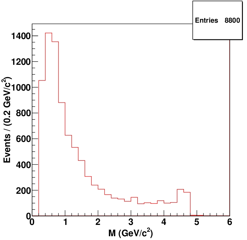
Figure 5: Sign–coded muon multiplicity distribution of additional muons found in $36.8^{\circ}$ cones around initial muons (left) and invariant mass distribution of all muons within cones which contain at least one additional muon (right), as predicted by the model with $\mu$ and $\tau$ number violating $X$ decays. We assume $X$ pair production from $q\bar{q}\rightarrow XX$; 91,191 of 20 million simulated events pass the two–muon cuts.

The number of ghost events in various experiments predicted by this model are listed in Table 3. The prediction for UA1 is very similar to that of the simple model discussed in Sec. 3, see Table 2. Mostly due to the larger $X$ mass, the number of ghost events expected at the fixed–target experiments is reduced, but at least for the $q\bar{q}$ production mechanism a significant number of events is again predicted.

Table 3: Expected number of ghost events for the model violating $\mu$ and $\tau$ number compared to the number of actually observed di–muon events. The normalization constants are $N^{\tau}_{gg}\approx(1.18\pm 0.06)\cdot 10^{-4}$ and $N^{\tau}_{q\bar{q}}\approx(2.1\pm 0.1)\cdot 10^{-3}$. $X$ pair production from gluon fusion requires branching ratios $73.39\,\mathrm{\%}$ for the 1–muon, $2.99\,\mathrm{\%}$ for the OS, $22.56\,\mathrm{\%}$ for the SS 2–muon and $1.06\,\mathrm{\%}$ for the 4–muon decay.

		# ghost events for		# of observed
Exp.	$\int{\cal L}dt$ [Nucl./pb]	$gg\rightarrow XX$	$q\bar{q}\rightarrow XX$	$\mu\mu$ events
CDF	$114.41\pm 6.51$	$84895\pm 4829$	$84895\pm 4829$	$84895\pm 4829$
UA1–a	0.108	$1.4\pm 0.1$	$5.9\pm 0.3$
UA1–b	0.6	$10.5\pm 0.6$	$34.8\pm 2.0$	880
UA1–c	4.7	$82.0\pm 4.7$	$266.8\pm 15.2$	2444
E605–a	$(1.14\pm 0.08)\cdot 10^{6}$	$2.0\pm 0.2$	$92.4\pm 8.4$	43663 (OS)
E605–b	$(2.7\pm 0.2)\cdot 10^{5}$	$1.2\pm 0.1$	$60.1\pm 5.7$	19470 (OS)
E772–a	$(5.8\pm 0.3)\cdot 10^{4}$	$6.6\pm 0.5$	$232.3\pm 18.1$	83080 (OS)
E772–b	$3.5\cdot 10^{5}$	$59.9\pm 3.5$	$2002.8\pm 116.4$	$\approx 450000$ (OS)
E789	$17.52\pm 1.89$	$2.7\pm 0.3$	$70.6\pm 8.6$	$71206\pm 287$ ($J/\psi$)
E866	$3.78\cdot 10^{5}$	$14.3\pm 0.8$	$471.5\pm 27.4$	$\approx 360000$ (OS)

4.3 Combined Model

The combination of the Breit–Wigner resonance in the $X$ pair production cross section with the $\tau$ and $\mu$ number violating $X$ decay modes enables us to reproduce the main characteristics of the observed ghost events. As in the previous Subsection we need $m_{X}=4.6\,\mathrm{GeV}$ to reproduce the in–cone multi–muon invariant mass distribution.

We saw above that the muons from $\tau$ decays and the directly produced muons in the two–muon decay modes are rather soft in this decay scenario. In order to reproduce the observed gradual decline of the multi–muon invariant mass distribution we therefore require larger values of $m_{Y}$ than in the scenario where $X$ decays conserve all lepton numbers separately. Specifically, if all $X$ pairs are produced from $q\bar{q}$ annihilation, we need $m_{Y}=\Gamma_{Y}=110\,\mathrm{GeV}$, whereas gluon fusion dominance requires $m_{Y}=\Gamma_{Y}=180\,\mathrm{GeV}$.

This in turn increases the number of $X$ particles produced with large $p_{T}$, and hence the efficiency with which additional muons pass the $p_{T}>2$ GeV cut. The branching ratios for the multi–muon channels therefore have to be adjusted downward relative to the model without Breit–Wigner factor. In case of $q\bar{q}$ production, we find 91.01 % for the 1–muon, 3.76 % for the OS, 2.86 % for the SS 2–muon, and 2.37 % for the 4–muon decay. In case of gluon fusion the branching ratios are 91.91 % for the 1–muon, 4.22 % for the OS, 3.25 % for the SS 2–muon, and 0.62 % for the 4–muon decay.

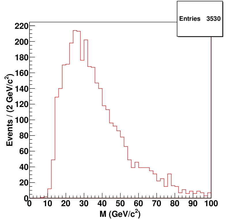
Figure 6: Sign–coded muon multiplicity distribution of additional muons found in $36.8^{\circ}$ cones around initial muons (left) and invariant mass distribution of all muons within events in which both cones contain each at least one additional muon (right), for $gg\rightarrow Y\rightarrow XX$ with the $\tau$ and $\mu$ number violating $X$ decay modes. 1,649,117 of 20 million generated events pass the two–muon cuts.

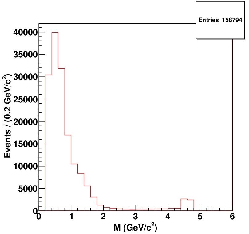
Figure 7: Simulated invariant mass distribution of all muons within cones which contain at least one additional muon, using $gg\rightarrow Y\rightarrow XX$ with $\mu$ and $\tau$ number violating $X$ decays. 1,649,117 of 20 million generated events pass the two–muon cuts.

There is a better reproduction of the muon multiplicity distribution for the gluon fusion compared to the quark–antiquark annihilation. Not only the entries in “1” and “10” are reproduced well, also the cones with two and three additional muons are in closer agreement with the measurement. The simulation results are shown in Fig. 6. In addition, the nearly complete absence of the 4–muon decay has the desirable side–effect that the peak at the mass of the $X$ particle in the simulation of Fig. 34a almost vanishes; see Fig. 7.

In this model around 25 (200) ghosts should have appeared at UA1 for gluon fusion ($q\bar{q}$ annihilation). As for the Breit-Wigner resonance with lepton number conserving $X$ decays, we do not expect ghost events in the data samples of the fixed–target experiments.

Recall that the poor acceptance of these experiments is a result of the cuts tailored for analyses of Drell–Yan production. If this cut can be relaxed, a significant number of ghost events could be detected even at fixed–target energies. In particular, a hypothetical fixed–target experiment with a center of mass energy of $38.8\,\mathrm{GeV}$ and an integrated luminosity of $1\cdot 10^{5}\,\mathrm{Nucl./pb}$ could probe the Breit–Wigner model with $\mu$ and $\tau$ number violating $X$ decay modes. If the initial muons each have a lab energy $E_{\mu}\geq 5\,\mathrm{GeV}$, we would expect $3276.0\pm 190.4$ ($408.9\pm 23.8$) ghost events for quark–antiquark annihilation (gluon fusion), if full angular acceptance is assumed. Hence, a fixed–target experiment with good spatial coverage can test even this most difficult model decisively, if the vertex resolution is sufficient to detect the decay length of the $X$ particles.

5 Summary and Conclusions

In this paper we investigated the question whether CDF “ghost” events could have been detected by experiments operating at lower energies. The answer to this question depends on the model chosen to describe the CDF data. We started by constructing a simple model, in which two light $X$ particles are produced in an S–wave, and decay into four–body final states containing at least one muon, with a decay length of 20 mm. As far as we can tell, this model describes the di–muon ghost sample fairly well; recall that this accounts for more than 90% of all ghost events. Since the $X$ particles are light, they could be produced not only at the CERN SpS collider, but also in fixed–target collisions at Fermilab. The latter should have accumulated hundreds to thousands of such events in their data, depending on whether $X$ pair production is dominated by gluon fusion or by $q\bar{q}$ annihilation. In half of these events both muons should have the same charge; there is very little physics background for such like–sign pairs at fixed–target energies, where $b\bar{b}$ production is suppressed (which can lead to like–sign pairs via $B^{0}-\overline{B^{0}}$ oscillations). Unfortunately the published analyses of di–muon data from these experiments are based on triggers that require the presence of two opposite–sign muons in the event. Some experiments evidently also recorded same–sign pairs, but the effective luminosities and efficiencies for these are not stated. On the other hand, at least one of the experiments, Fermilab E789, should have had no trouble detecting the typical $X$ decay length of several cm.

However, this simple model does not reproduce the ghost events with more than two muons very well. It does not predict sufficiently many secondary muons with the same charge as the primary one, and it predicts a too steep fall–off of the multi–muon invariant mass distribution. The first problem can be cured by allowing $X$ decays to violate $\mu$ and $\tau$ number, still respecting the overall lepton number, while the second problem can be solved by assuming that $X$ pair production proceeds via a very broad resonance $Y$. This more complicated model still predicts that the UA1 di–muon sample should contain an appreciable number of ghost events; however, these would be overwhelmed by di–muon events from conventional sources, in particular from $b\bar{b}$ production, unless the long decay length of the $X$ particles could be detected. Moreover, this model predicts that few or no ghost events should be contained in the Fermilab fixed–target di–muon data. However, these data were subjected to angular cuts that isolate Drell–Yan events, but are very inefficient for ghost events. We saw that a fixed–target experiment with good angular coverage and sufficient tracking resolution to detect the finite $X$ decay length should be able to decisively probe even this more complex model.

Given the spectacular nature of the ghost events, it seems unlikely to us that they would have escaped detection, had they been produced at rates similar to those predicted by our simple model. However, a proper analysis can only be performed by the experimental groups themselves; this is true in particular in view of the apparently quite complicated acceptances of these experiments. We hope that this paper, and the ghost models we constructed and embedded into HERWIG++, will facilitate such analyses.

Acknowledgments

NB wants to thank the “Bonn-Cologne Graduate School of Physics and Astronomy” and the “Universität Bonn” for financial support.

References

- [1] T. Aaltonen et. al., arXiv:0810.5357v2 [hep-ex].
- [2] M. Bähr et. al., Eur. Phys. J. C 58, 639 (2008), arXiv:0803.0883 [hep-ph].
- [3] C. Albajar et al., Phys. Lett. B 186, 237 (1987); C. Albajar et al., Phys. Lett. B 256, 121 (1991).
- [4] G. Moreno et. al., Phys. Rev. D 43, 2815 (1991).
- [5] P. L. McGaughey et. al., Phys. Rev. D 50, 3038 (1994); P. L. McGaughey et. al., Phys. Rev. D 60, 119903 (1999); D. M. Alde et. al., Phys. Rev. Lett. 64, 2479 (1990).
- [6] D. M. Janson et. al., Phys. Rev. Lett. 74, 3118 (1995).
- [7] E. A. Hawker et. al., Phys. Rev. Lett. 80, 3715 (1998); R. S. Towell et. al., Phys. Rev. D 64, 052002 (2001).
- [8] T. Müller, Nucl. Instr. Meth. A 252, 387 (1986).