The Properties of X-ray Cold Fronts in a Statistical Sample of Simulated Galaxy Clusters

Abstract

We examine the incidence of cold fronts in a large sample of galaxy clusters extracted from a (512$h^{-1}$Mpc) hydrodynamic/N-body cosmological simulation with adiabatic gas physics computed with the Enzo adaptive mesh refinement code. This simulation contains a sample of roughly 4000 galaxy clusters with M$\geq 10^{14}M_{\odot}$ at $z$=0. For each simulated galaxy cluster, we have created mock 0.3-8.0 keV X-ray observations and spectroscopic-like temperature maps. We have searched these maps with a new automated algorithm to identify the presence of cold fronts in projection. Using a threshold of a minimum of 10 cold front pixels in our images, corresponding to a total comoving length $L_{cf}>156h^{-1}kpc$, we find that roughly 10-12% of all projections in a mass-limited sample would be classified as cold front clusters. Interestingly, the fraction of clusters with extended cold front features in our synthetic maps of a mass-limited sample trends only weakly with redshift out to $z$=1.0. However, when using different selection functions, including a simulated flux limit, the trending with redshift changes significantly. The likelihood of finding cold fronts in the simulated clusters in our sample is a strong function of cluster mass. In clusters with $M>7.5\times 10^{14}M_{\odot}$ the cold front fraction is 40-50%. We also show that the presence of cold fronts is strongly correlated with disturbed morphology as measured by quantitative structure measures. Finally, we find that the incidence of cold fronts in the simulated cluster images is strongly dependent on baryonic physics.

1. Introduction

With the advent of high resolution X-ray imaging using space-based observatories, in particular Chandra, unexpected discontinuous X-ray features in galaxy clusters were discovered. The expected appearance of shocks was supplemented by the appearance of cold fronts, features that do not exhibit a pressure jump, in contrast to shocks, but have jumps in surface brightness and temperature in opposing directions (for review see Markevitch & Vikhlinin, 2007). Temperature jump ratios (from one side of the feature to the other) in typical cold fronts range from factors of 50% to factors of a few, with corresponding (but reversed) inferred density jumps. Because of the pressure continuity across these features, they are typically described as contact discontinuities. Early classic cold front examples include Abell 3667 (Vikhlinin et al., 2001a) and Abell 2142 (Markevitch et al., 2000). The properties of cold fronts have turned out to provide excellent constraints on the physics of the intracluster medium (ICM). For example, the extremely sharp edge (typically narrower than the Coulomb mean free path) between the cold and hot sides of the features places limits on the effectiveness of conduction across the edge (e.g., Ettori & Fabian, 2000; Asai et al., 2004). The apparent lack of fluid instability growth at the interface also suggests some physical process that stabilizes the edge, perhaps the draping of magnetic fields (Vikhlinin et al., 2001b; Lyutikov, 2006; Asai et al., 2007; Takizawa, 2008).

Following the early discoveries of cold fronts, many other clusters have been identified as hosting cold fronts (e.g., Mazzotta et al., 2001; Markevitch et al., 2002; Dupke & White, 2003; Hallman & Markevitch, 2004; Johnson et al., 2010). Statistics of cold fronts in clusters have been calculated using data from the Chandra archive (Owers et al., 2009) and from flux-limited samples using XMM-Newton (Ghizzardi et al., 2006, 2010) and Chandra (Markevitch et al., 2003). The main results are that in flux-limited samples, anywhere between 40% and 87% of clusters are found to host cold fronts (Ghizzardi et al., 2006, 2010) depending on the redshift range explored. Also, a large fraction of cool core clusters ($\sim$67%) host cold fronts (Markevitch et al., 2003). Recent work also suggests that the appearance of cold fronts is strongly correlated with cluster mergers (Owers et al., 2009; Ghizzardi et al., 2010).

Numerical hydrodynamic simulations of idealized cluster mergers (e.g., Roettiger et al., 1999; Heinz et al., 2003; Takizawa, 2005; Ascasibar & Markevitch, 2006; Mastropietro & Burkert, 2008; Springel & Farrar, 2007; ZuHone & Markevitch, 2009) as well as cosmological simulations (e.g., Nagai & Kravtsov, 2003; Bialek et al., 2002; Mathis et al., 2005; Tittley & Henriksen, 2005) appear to reproduce the properties of all types of observed cold fronts naturally in the process of mergers. Recent studies have begun to separately classify two types of cold fronts, the first being “merger” cold fronts, where the system is obviously disturbed in X-ray morphology, and clearly undergoing a current major merger, and so-called “sloshing” cold fronts (Markevitch et al., 2001) in apparently otherwise relaxed cool-core clusters. This distinction is somewhat artificial, as simulations show that both cold front types are associated with mergers, or in the case of sloshing, at least a close pass of a subcluster.

Simulation studies indicate that cold fronts arise from one of a few physical scenarios. First, and most obvious are the so-called merger-type cold fronts. In these scenarios, two objects merge, at least one a massive cluster. In the early stages, while the merging subclusters are approaching, their relative velocity is supersonic (in the cluster gas) and drives shocks. In the simplest scenario, the ram pressure associated with the relative velocity of the subcluster in the gas of the main cluster pushes the subcluster gas out of the dark matter potential well. Once the gas separates from the dark matter potential, it expands adiabatically and cools, resulting in the cold front feature. In this scenario, cold fronts should always be associated with shocks, which may also be visible in the ICM adjacent to the cold front. Depending on when in the process of merging the cold front is observed, the relative positions of cold gas, dark matter, and shocks can vary.

The sloshing type cold fronts are observed typically in cool core clusters, and appear at small cluster radius (R$<100kpc$). These clusters otherwise appear relaxed dynamically, leading to the separate classification from merger type cold fronts. There is no obvious evidence of merging in these clusters in the X-ray images, but simulations that reproduce cold fronts of this type show that they are also caused by dynamical interactions. In simulations, a near pass of a subcluster pulls the cluster mass away from the original center position, and as the subcluster moves away, the central baryonic material rocks back and forth in the dark matter potential. This creates a characteristic spiral shaped cold front near the center of the cool core cluster.

Both the simulation work referenced here and recent theoretical study (e.g., Lyutikov, 2006; Birnboim et al., 2009; Keshet et al., 2009) have made significant progress toward understanding the process by which cold fronts form in galaxy clusters and the detailed physics that determines their observed properties. What has not been attempted to date is an estimate of the predicted incidence of cold fronts in clusters from fully cosmological numerical hydro/N-body simulations with large (N $>1000$) samples. The appearance of merger-type cold fronts is governed by both the merger rate of cluster scale systems, as well as the gas dynamics and more subtle effects like projection angle. Therefore, in order to determine how many clusters we expect to have cold fronts at a given epoch, or mass limit, or depth of observation, a statistical treatment is required. Though idealized merger scenarios, or small samples simulated at high resolution are critical to understanding the range of cold front formation, they neglect to examine the full ranger of mergers in large scale structure. Fully cosmological simulations, like the ones performed for this study, create realistic merger histories, including multiple mergers. From these simulations we can gain valuable insight about the process of cold front formation and evolution over a large statistical sample of galaxy clusters.

The outline of this paper is as follows. In Section 2, we describe the setup and analysis of the Enzo simulations. In Section 3 we discuss the method of cold front identification. In Section 4 we describe our major results. In Section 5 we describe briefly the effects of numerical resolution and baryonic physics. Finally, in Section 6, we discuss and summarize our results.

2. Simulation Setup and Analysis

The main statistical results come from the so-called Santa Fe Light Cone (SFLC) simulation, described in Hallman et al. (2007), Skillman et al. (2008) and Hallman et al. (2009). This calculation is performed with ‘Enzo’, a publicly available adaptive mesh refinement (AMR) cosmology code developed by Greg Bryan and colleagues (Bryan & Norman, 1997a, b; Norman & Bryan, 1999; O’Shea et al., 2004, 2005). The specifics of the Enzo code are described in detail in these papers (and references therein).

The Enzo code couples an N-body particle-mesh (PM) solver (Efstathiou et al., 1985; Hockney & Eastwood, 1988) used to follow the evolution of a collisionless dark matter component with an Eulerian AMR method for ideal gas dynamics by Berger & Colella (1989), which allows high dynamic range in gravitational physics and hydrodynamics in an expanding universe.

This simulation is set up as follows. We initialize our calculation at $z=99$ assuming a cosmological model with $\Omega_{m}=0.3$, $\Omega_{b}=0.04$, $\Omega_{\Lambda}=0.7$, $h=0.7$ (in units of 100 km/s/Mpc), $\sigma_{8}=0.9$, and using an Eisenstein & Hu (1999) power spectrum with a spectral index of $n_{s}=1$. The simulation is of a volume of the universe 512 h^-1 Mpc (comoving) on a side with a $512^{3}$ root grid. The dark matter particle mass is $7.3\times 10^{10}$ h^-1 M_⊙. The simulation was then evolved to $z=0$ with a maximum of $7$ levels of adaptive mesh refinement (a maximum spatial resolution of $7.8$ h^-1 comoving kpc), refining on dark matter and baryon overdensities of $8.0$. The equations of hydrodynamics were solved with the Piecewise Parabolic Method (PPM) using the dual energy formalism. This simulation is performed using adiabatic physics only. It has become clear from observations that additional non-gravitational physics is important in the evolution of the ICM. However, this run models a large volume with high peak resolution, which is only now becoming possible to calculate while including additional baryonic physics. It has the advantage of generating a cluster sample with thousands of massive clusters, allowing us to explore a wide range of cluster interactions that result in cold fronts.

Analysis was performed on 11 data outputs between $z=1$ and $z=0.0$ (spaced with $\delta$z = 0.1) in an identical way. The HOP halo-finding algorithm (Eisenstein & Hut, 1998) was applied to the dark matter particle distribution to produce a dark matter halo catalog (as in Hallman et al., 2007). For each output, we calculate bulk properties (e.g., total mass, X-ray luminosity), radial profiles, and projected images (along 3 orthogonal axes) of each simulated cluster in a variety of physical and observable properties. Spherically-averaged, mass-weighted radial profiles of various baryonic and dark matter quantities including density, temperature, and pressure were generated for every halo in the catalog with an estimated halo mass greater than $4\times 10^{13}$ M_⊙. These radial profiles were used to calculate $M_{200}$ and $R_{200}$. $M_{200}$ refers to the total mass inside a radius of $R_{200}$, the radius at which the overdensity average inside the sphere centered on the cluster is 200 times the critical density. We then generate synthetic X-ray images for clusters in the sample with $M_{200}>10^{14}M_{\odot}$. We then run our automated cold front finder on three orthogonal projections of each cluster. A histogram of the size of the mass-limited cluster sample as a function of redshift is shown in Figure 1.

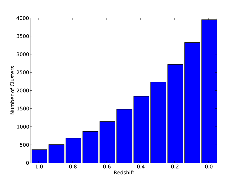
Figure 1.— Histogram of number of clusters with $M>10^{14}M_{\odot}$ in the comoving volume as a function of redshift. Shows the sample size used for the cold fronts analysis.

2.1. Testing the Effect of Baryonic Physics

For the purpose of understanding the impact of additional baryonic physics on the cold front incidence, we have analyzed two additional simulations. Each of the two simulations have identical simulation volumes, initial conditions, and cosmology. The simulated volume is a $128h^{-1}$ comoving Mpc cube, with 256³ root grid zones and 256³ dark matter particles. Each run is allowed to refine to a maximum of 5 AMR levels, and the refinement criteria are overdensity of 8.0 in either the dark matter or the gas (with respect to the mean on the parent level). This gives the run a peak spatial resolution of 15.6$h^{-1}$kpc. The dark matter particle mass is $9.0\times 10^{9}$ h^-1 M_⊙ and the mean baryon mass resolution is $1.4\times 10^{9}$ h^-1 M_⊙, a factor of 8 improvement over the SFLC run used for our main analysis. For these runs, we use a cosmological model with $\Omega_{m}=0.27$, $\Omega_{b}=0.044$, $\Omega_{\Lambda}=0.73$, $h=0.7$ (in units of 100 km/s/Mpc), $\sigma_{8}=0.9$, and using a power spectrum with a spectral index of $n_{s}=0.97$. These values are changes from our previous run, to match WMAP5 cosmological parameters. Therefore, there are multiple changes to these simulations from the SFLC, including the mass and spatial resolution, baryonic physics, and cosmological parameters. The most relevant changes to the cosmology are a slight reduction in the value of $\Omega_{m}$ and a slight increase in the value of $\Omega_{\Lambda}$. However, in this work, we endeavor to merely compare our two runs where everything is identical except baryonic physics, to examine the impact.

The two additional simulations presented here are identical in terms of the initial conditions and simulation properties, except that one has only adiabatic and gravitational physics, and the other includes a prescription for radiative cooling of the gas using non-equilibrium cooling and chemistry for H and He, Cloudy (Ferland et al., 1998) for the metal cooling, and star formation including thermal and metal feedback from supernovae as detailed in Cen & Ostriker (1999). The cooling plus star formation and feeback run includes a spatially uniform but time-varying ultraviolet (UV) radiation background (Haardt & Madau, 1996). We turn on the UV background at a redshift z = 7. For the metal line cooling, we interpo- late from a grid of data made with Cloudy. For redshifts z $>$ 7, we use a similar grid of heating and cooling data, without the influence of the UV radiation background, assuming collisional ionization only (for more details, see Smith et al., 2008, 2010). Additionally, we have highly time-resolved data outputs for these calculations, allowing us to examine the time history and origin of cold fronts in the simulated clusters in detail. In this paper, we examine only the general incidence of cold fronts in these simulations, and leave a study of the detailed properties of the cold fronts, as well as a full convergence study, to future work.

For our simulation with purely adiabatic physics (CC-Adia), and the identical run with additional baryonic physics (CC-OTH), the data outputs and analysis are identical. We perform the same analyses as done for the SFLC simulation.

3. Cold Front Identification and Analysis

The identification of X-ray cold fronts in the synthetically observed numerical clusters is done via a relatively simple algorithm, which is designed to roughly match the observational (by eye) identification, but in an automated way.

For this study, we focus on the identification of X-ray cold fronts, characterized as features which are both colder and brighter than the surrounding intracluster medium. This identification is made from projected images of the clusters of the spectroscopic-like temperature ($T_{sl}$) (see Mazzotta et al., 2004; Rasia et al., 2005), and the 0.3-8.0 keV X-ray surface brightness calculated using the Cloudy code (Ferland et al., 1998). The spectroscopic-like temperature has been determined to be an accurate proxy for the measured X-ray spectral temperature (Rasia et al., 2005). We are not using the volume integral of the spectroscopic-like temperature as in Rasia et al. (2005), but are using the same weighting for the line of sight integral in order to make mock temperature maps. This weighting has been shown to reproduce the fitted spectral temperature better than standard emission weighting or mass weighting. The calculation of $T_{sl}$ for our projected maps is

$$T_{sl}=\frac{\int n^{2}T^{a}/T^{0.5}dl}{\int n^{2}T^{a}/T^{1.5}dl},$$ (1)

where a=0.75.

For each image, we step in each row or column of the pixel map, and look for jumps in the surface brightness and temperature which are above a threshold value, and are opposite in sign. The jump thresholds are

$$S_{x,1}/S_{x,2}>2.0,$$ (2)

$$T_{sl,2}/T_{sl,1}>1.4,$$ (3)

where the numerical subscripts indicate the 2 opposing sides of the edge in temperature and surface brightness. Note that the jump in surface brightness is in the opposite direction of the jump in temperature. Observed cold fronts have temperature jumps from factors of 50% to factors of a few, so this threshold should be sufficient to recover the observed distribution. The threshold jump strengths are designed to be roughly continuous in pressure, as the fixed band X-ray surface brightness is only weakly dependent on temperature and depends on the electron density squared. Therefore a surface brightness jump of 2.0 is roughly equivalent to a projected density jump of 1.4. We also limit the identification of cold fronts to the area within a radius of $r_{500}$ projected on the sky, where $r_{500}$ is the radius within which the mean overdensity of the cluster is 500 times the value of $\rho_{c}$, the critical density of the universe. This radius is chosen since it is representative of the part of massive galaxy clusters that can typically be observed with standard exposures using current X-ray telescopes.

We expect the number of cold fronts and the size of the jumps to be a lower limit to the true number in the simulation. This results from a number of factors. First, the effects of projection on the detection of cold fronts must be considered. Like shocks in galaxy clusters, the detection is strongly orientation dependent. Edge-on orientations lead to much more detectable shocks and cold fronts, face-on oriented features are basically undetectable via these methods. Second, because of both orientation and potential spreading of the discontinuity over several numerical grid cells, the jump may span 2-3 pixels. Our method in that case may miss a more gradual jump, or detect it with a smaller ratio of temperature and surface brightness across the feature. The first effect (projection) is not considered directly in this study, since we only wish to compare the observed incidence of cold fronts to the simulated incidence, and real cluster observations suffer the same effect. We partially compensate for this effect by using multiple orthogonal projections of each cluster, but this doesn’t impact the fractional incidence, as we count each projection as an independent image. The second set of effects is more challenging to correct. In this study we have experimented with checking for features matching our criteria across both 2 and 3 pixels. The main result of that experiment is that the overall statistics are not strongly dependent on the number of pixels across which the jump is considered. This results from the fact that jumps that are identified in a single pixel jump are also typically identified in 2-3 pixels as well. For this same reason it is not effective to include all jumps of 1, 2, and 3 pixels for instance in our analysis due to redundant detections of the same features. For the purposes of this study, we consider the incidence of cold fronts detected via this method to be lower limits, and the jumps may also be underestimated (individually). Based on our tests, we expect the overall statistics to be largely unaffected, though it will be explored in more detail in our later work.

Because cold fronts are extended features in the X-ray, we anticipate that their incidence will not be strongly dependent on grid resolution. The incidence of cold fronts may however be somewhat dependent on the baryonic physics of the simulation, as well as the mass resolution. Mass resolution of the simulation results in a higher number of resolved subclusters, increasing the rate of mergers. Although previous work has shown that cold fronts certainly appear in adiabatic simulations, purely adiabatic processes may not be the only mechanisms for cold front creation. The so-called “sloshing” cold fronts may result from gas which has radiatively cooled in the centers of clusters oscillating in the dark matter potential in response to mergers. These sloshing features appear in observed clusters with strong central entropy gradients (e.g., Markevitch et al., 2003; Ghizzardi et al., 2010). In this work we make no distinction between sloshing and merger-type cold fronts, we merely identify all features that match the cold front criteria specified above. In our adiabatic simulations, because we do not get strong core entropy gradients (as are seen in the presence of strong radiative cooling), we expect our cold fronts to be of the merger type in this simulation.

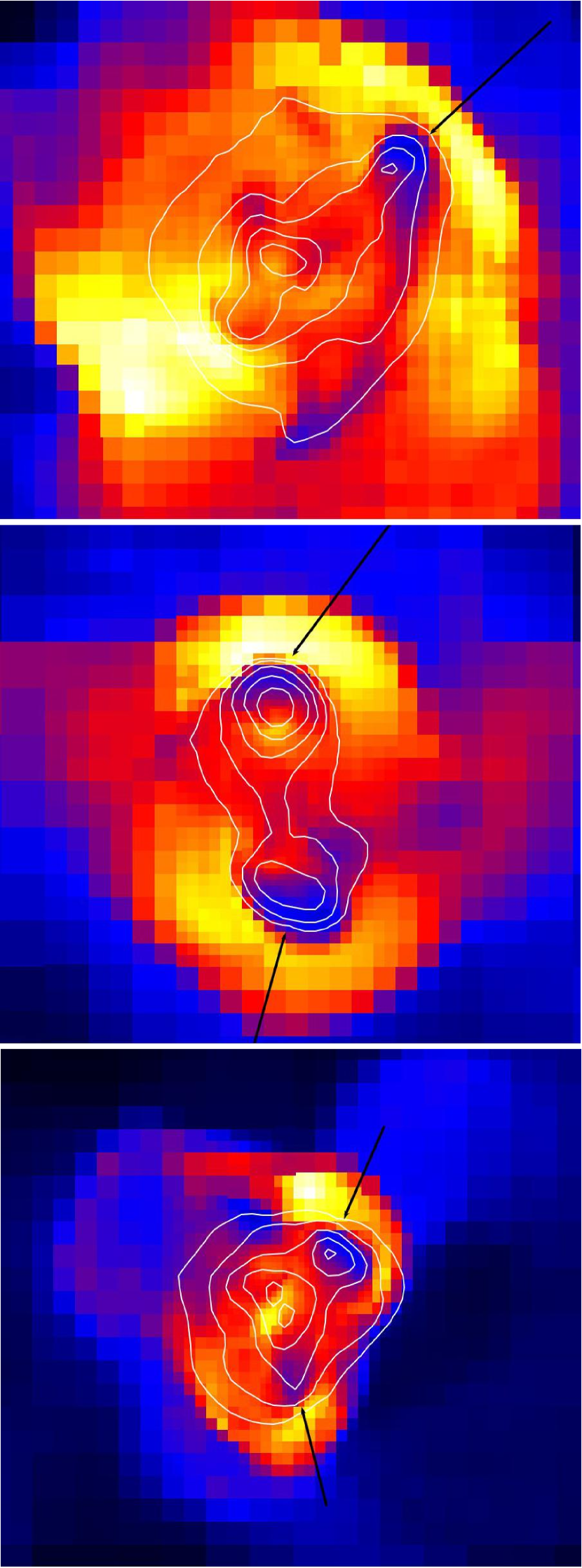
Figure 2.— Representative cold fronts from the numerically simulated clusters at $z$=0, with mass (from top to bottom) of 3.1$\times 10^{15}M_{\odot}$, 1.4$\times 10^{15}M_{\odot}$, and 1.2$\times 10^{15}M_{\odot}$. Image quantity is $T_{sl}$, contours are 0.3-8.0 keV X-ray surface brightness. Field of view is roughly 3h^-1 Mpc. Image scale goes from $T\sim$3keV (blue) to $T\sim$10-12keV (yellow-white). Arrows indicate locations identified by the automated finder as cold fronts.

4. Results

4.1. Incidence of Cold Fronts in Simulated Clusters

The first result of the cold front identification is that in the adiabatic simulation, for the sample of all clusters with $M\geq 10^{14}M_{\odot}$ out to $z=1$, 12% of images have 10 or more cold front pixels, 5% have 20 or more, and roughly 1% have 50 or more. At $z$=0 in our adiabatic simulation, we have 116 images with more than 50 cold front pixels. In these images, there are clear, unambiguous cold fronts spanning large areas of the cluster projection (see Figure 2). Figure 3 shows the result of counting clusters above some minimum pixel count identified as cold fronts. This is equivalent to measuring the comoving total length of cold front features in each image, as each pixel has a constant comoving size in all of these images. In the figure, we plot the trend as a function of redshift for clusters with at least 10 pixels ($L_{cf}>156h^{-1}$ kpc total) identified as a cold front, 20 pixels ($L_{cf}>312h^{-1}kpc$) and 50 pixels ($L_{cf}>780h^{-1}kpc$). These numbers are arbitrary, and designed purely to show the general redshift trend. It is clear from this plot that there is only a weak trend in the incidence of cold fronts as a function of redshift out to $z=$1.

The choice of a threshold in cold front pixels or comoving length of features is fairly arbitrary, but identification of one pixel with cold front criteria is not particularly interesting. First, it is quite possible to have spurious cold pixels due to line-of-sight superpositions. Additionally, cold fronts are extended features, and so in these images at least several pixels need to be associated in order for a true identification to take place.

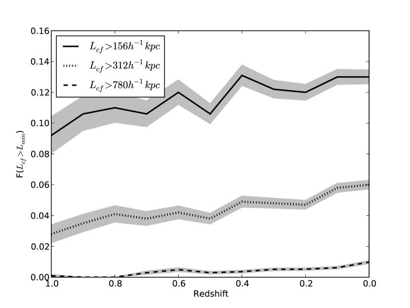
Figure 3.— Fraction of clusters displaying a cold front as a function of redshift. Solid line is clusters with more than 10 cold front pixels (total $L_{cf}>156h^{-1}$kpc comoving), dotted line is for 20 cold front pixels ($L_{cf}>312h^{-1}kpc$), the dashed line represents 50 pixels ($L_{cf}>780h^{-1}kpc$) identified as cold fronts in the image. Gray regions are 1$\sigma$ Poisson error bars. Note the relatively flat redshift trend.

Another interesting statistic is the incidence of cold fronts in simulated clusters as a function of mass. For this case, we take clusters with at least 10 identified cold front pixels, which as described earlier is equivalent to the combined length of cold fronts $L_{cf}>156h^{-1}kpc$. We combine the result for all clusters from $1.0\geq z\geq 0.0$ in Figure 4. What we see here is that the likelihood of finding extended cold fronts in clusters increases with mass. There are several possible interpretations for this result. The first, which is that this is a real physical trend, is that more massive clusters form in more dense local environments, leading to more activity from mergers and accretion, increasing the number of cold fronts generated. A second possibility is that because smaller clusters are smaller in projection, and we have a fixed comoving pixel scale, they are less likely to have extended cold front features purely because of resolution effects. This effect is compounded by the larger cross section for mergers for the larger clusters, generating a higher likelihood for a merger of a given size in that projected volume at any time. It is legitimate to ask how the sample can have only a weak trend in cold front incidence with redshift, yet have a strong mass trend. Given the hard lower mass limit at each redshift, the distribution of clusters as a function of mass in each redshift bin is different. In other words, the clusters selected at each redshift with an identical mass cutoff do not represent the same part of the halo mass function at each redshift. This effect may contribute to the result shown here. We expect that if cold fronts are related to merger activity (as is indicated by simulation studies) that their incidence should trend with redshift, as large-scale structure grows, and the merger rates change as a function of time.

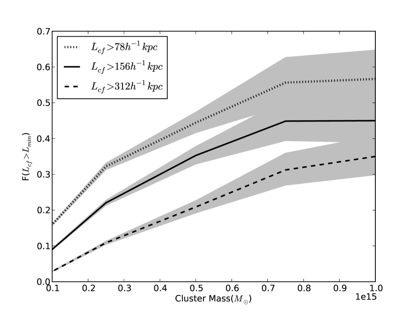
Figure 4.— Trend of cold front incidence as a function of mass for clusters from $1.0\geq z\geq 0.0$. Solid line is for clusters counted as cold front clusters if they have at least 10 identified cold front pixels, corresponding to a total cold front length $L_{cf}>156h^{-1}kpc$ comoving, within a projected radius of $r_{500}$. These pixels are not necessarily contiguous. Also plotted for comparison are the trends with a limit of half as many pixels ($L_{cf}>78h^{-1}kpc$, dotted line) and twice as many ($L_{cf}>312h^{-1}kpc$, dashed line). Note the steep trend in mass, and the flattening at high mass ($M>7.5\times 10^{14}M_{\odot}$). Gray regions are 1$\sigma$ Poisson error bars.

In our above calculation of the fraction of cold front clusters as a function of cluster mass, we include clusters from all redshifts. Does this trend with mass vary as a function of redshift? Figure 5 shows the fraction of cold front clusters as a function of mass for 4 redshift bins in the simulation. The result is that the trend with mass is nearly identical for all redshifts, albeit with slight shifting in the upper mass bins due to small numbers. Effectively, clusters at all redshifts show an identical trend of increasing fraction of clusters with cold fronts with cluster mass.

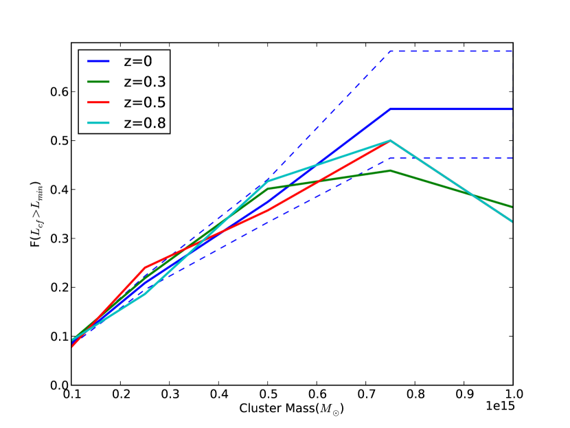
Figure 5.— Fraction of clusters with $L_{cf}>156h^{-1}kpc$ as a function of cluster mass for 4 different redshift bins, $z$=0, $z$=0.3, $z$=0.5 and $z$=0.8. Blue dashed lines are for 1$\sigma$ Poisson errors for the $z$=0 sample. Poisson errors overlap for all redshifts at the high mass end.

4.2. Selection Effects

Using a mass or flux-selected sample of galaxy clusters to study trends as a function of redshift is an inherently flawed method, as has been pointed out by many investigators. The most well known bias in flux-limited samples is the Malmquist bias, where your survey progressively selects brighter objects at greater distances. For galaxy clusters this has the effect of choosing the higher mass objects at higher redshift. Our sample has a bias working in the opposite direction, which is that we are selecting a mass-limited sample from all redshifts. Effectively we are sampling objects in different parts of the halo mass function at each redshift, not objects that at high redshift would be the precursors to the objects at low redshift in our sample. The result of such a selection is that true evolutionary effects as a function of redshift can easily be masked. One solution is to use a method similar to Hart et al. (2009), selecting objects along an evolutionary “road”, such that objects selected at low redshift are, in a statistical sense, the children of the objects at higher z.

To understand our result of the incidence of cold fronts having only weak trending with redshift, we sort our cluster sample in two additional ways. The first method we choose here is to use a Press-Schechter (Press & Schechter, 1974) mass function analysis to select a lower mass cutoff at each redshift corresponding to halos of the same rarity in large scale structure. This threshold choice effectively follows the same cluster population as a function of redshift, allowing us to see evolutionary trends in the incidence of cold fronts.

Our selection is done by calculating the value of $\sigma_{M}$, the RMS density fluctuation, as a function of cluster mass and redshift. We then choose a lower mass limit for our sample such that $\sigma_{M}$ is a constant with redshift. This choice is motivated by the analytic expressions for the cluster mass function, both derived from linear theory and fit empirically to numerical simulations. The derivations below are taken from the cited references as well as Hallman et al. (2007). The comoving number density of clusters as expressed by Jenkins et al. (2001) is

$$\frac{dn}{dm}(M,z) = -0.315\frac{\rho_{0}}{M}\frac{1}{\sigma_{M}}\frac{d\sigma_{M}}{dm}$$ (4)

$$exp \left[-|0.61-log(D(z)\sigma_{M})|^{3.8}\right]$$

where $\sigma_{M}$ is the RMS density fluctuation, computed on mass scale $M$ from the $z=0$ linear power spectrum (Eisenstein & Hu, 1999), $\rho_{0}$ is the mean matter density of the universe, defined as $\rho_{0}\equiv\Omega_{m}\rho_{c}$ (with $\rho_{c}$ being the cosmological critical density, defined as $\rho_{c}\equiv 3H_{0}^{2}/8\pi G$), and $D(z)$ is the linear growth function, given by this fitting function:

$$D(z)=\frac{1}{1+z}\frac{5\Omega_{m}(z)}{2}$$

$$\left\{\Omega_{m}(z)^{4/7}-\Omega_{\Lambda}(z)+[1+\frac{\Omega_{m}(z)}{2}][1+\frac{\Omega_{\Lambda}(z)}{70}]\right\}^{-1}$$ (5)

(Carroll et al., 1992), with $\Omega_{m}(z)$ and $\Omega_{\Lambda}(z)$ defined in the typical way in a flat universe with cosmological constant. For the details of the calculation, see Hallman et al. (2007).

The RMS amplitude of the density fluctuations as a function of mass and redshift, smoothed by a spherically symmetric window function with comoving radius R, can be computed from the matter power spectrum using:

$$\sigma^{2}(M,z)=\int_{0}^{\infty}\frac{dk}{k}\frac{k^{3}}{2\pi^{2}}P(k,z)|\mbox{\~{W}}_{R}(k)|^{2}$$ (6)

where $\mbox{\~{W}}_{R}(k)$ is the Fourier transform of the real-space top hat smoothing function:

$$\mbox{\~{W}}_{R}(k)=\frac{3}{k^{3}R^{3}}\left[sin(kR)-kRcos(kR)\right]$$ (7)

We choose the value of $\sigma_{M}$ for our lower limit from the lower mass limit at $z$=1, which is $M_{limit}$ = 10${}^{14}M_{\odot}$. Simply put, we use a constant $\sigma_{M}$ limit, and take all clusters in the simulation above that lower mass limit at each redshift. The result is shown in Figure 7.

Figure 6.— Mass limits derived from the $\sigma_{M}$- and flux-limited cases described in the text. In each case, the sample of clusters used in the analysis are those above the specified mass limit at each redshift.

The result clearly changes the sense of the redshift trend from the mass-limited sample. Now we see an increase in the fraction of clusters with cold fronts as a function of time. This selection should allow us to isolate evolutionary effects, as we are sampling the same part of the mass function at each redshift. The fraction generally increases as we move forward in time, which is not particularly surprising, since the result of our sample selection is that the lower mass limit goes up with time. As we have shown, the fraction of clusters with cold fronts is a strong function of mass. What is puzzling is the dip in the fraction at $z$=0.2. It is not entirely clear how to explain the appearance of this feature, though it is possible that a varying lower mass limit may create arbitrary features.

The second additional selection mimics an observational selection by a flux limit. Since this simulation has only adiabatic physics, and as such does not predict the X-ray luminosity accurately, we do not use the total X-ray emission calculated from the physical properties of the simulated clusters. Instead, we take a simple approach, using observationally determined X-ray scaling relations to create a mass limit as a function of redshift for our sample.

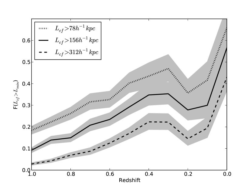
Figure 7.— Trend in redshift of clusters with the indicated $L_{cf}$ for each line. Dotted line indicates $L_{cf}>78h^{-1}kpc$, solid line is for our fiducial limiting $L_{cf}>156h^{-1}kpc$, dashed line is for $L_{cf}>312h^{-1}kpc$. This plot uses a lower mass limit in each redshift bin drawn from a constant $\sigma_{M}$ limit, highlighting evolutionary trends in the same set of clusters through time. Included are the trends with the same limiting length of cold front pixels as in previous Figure 4. Gray regions indicate 1$\sigma$ Poisson error bars.

We take the X-ray scaling relation fit by Mantz et al. (2009), a simple power law

$$l(m)=\beta_{0}^{lm}+\beta_{1}^{lm}m,$$ (8)

where

$$l=log_{10}\left(\frac{L_{500}}{E(z)10^{44}ergs^{-1}}\right),$$ (9)

and

$$m=log_{10}\left(\frac{E(z)M_{500}}{10^{15}M_{\odot}}\right).$$ (10)

$E(z)$ is defined in the usual way in a flat $\Lambda$CDM universe,

$$E(z)=(\Omega_{m}(1+z)^{3}+\Omega_{\Lambda})^{1/2},$$ (11)

and $\beta_{0}^{lm}$ and $\beta_{1}^{lm}$ are the fitted parameters. Mantz et al. (2009) find those parameters to be $\beta_{0}^{lm}$ = 0.82$\pm$0.11, and $\beta_{1}^{lm}$ = 1.29$\pm$0.07 by fitting to the X-ray luminosity function. We use the flux limit from the ROSAT-ESO Flux-Limited X-ray sample (REFLEX; Böhringer et al., 2001). In this case, we are not interested in any particular flux limit, we simply want to show the effect of sample selection on the cold front statistics. The REFLEX flux limit is 2.0$\times$10${}^{-12}ergs^{-1}cm^{-2}$. At each redshift from the simulation, we calculate the X-ray luminosity appropriate to the flux limit, then calculate the cluster mass associated to that luminosity using the scaling relation from Mantz et al. (2009). For the $z$=0 clusters, we use $z$=0.05 to calculate the value of $D_{L}$ and the flux. We compare the lower mass limits as a function of redshift in the $\sigma_{M}$- and flux-limited cases in Figure 6.

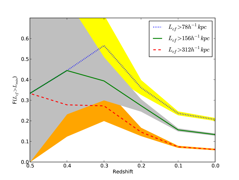
Figure 8.— Trend in redshift of clusters with the indicated $L_{cf}$ for each line. This plot uses a lower mass limit in each redshift bin drawn from a flux limit (from the REFLEX cluster sample) and the X-ray scaling relations from Mantz et al. (2009). Each cluster mass is converted to a luminosity from the scaling relations, and then a flux given its luminosity distance. Included are the trends with the same limiting length of cold front pixels as in previous Figures 4 and 7. This includes our fiducial limiting $L_{cf}>156h^{-1}kpc$ (solid green line), as well as limits of half the fiducial length (dotted, blue line) and twice the fiducial length (dashed, red line). Yellow, gray, and orange regions are 1$\sigma$ Poisson error bars for the $L_{cf}>78h^{-1}kpc$ line, $L_{cf}>156h^{-1}kpc$ line and the $L_{cf}>312h^{-1}kpc$ line respectively.

The resulting statistics of cold front incidence are shown in Figure 8. Note that this plot only shows fractions of clusters with cold fronts from $z$=0.5 to $z$=0, as at this flux limit, we have no clusters in our simulation above the appropriate mass at higher redshifts. In any case, it is clear that a flux limited selection results in a very different picture of the incidence of cold fronts when compared either to the mass-limited or $\sigma_{M}$-limited cases. The flux limit, of course, preferentially selects higher mass objects at higher $z$. As we have seen in our analysis of the incidence of cold fronts as a function of mass, it is a strong function of mass, so this result is not surprising. In a flux limited sample, we should expect the highest fraction of cold front clusters at high redshifts (since we select the highest mass clusters there), and it should decrease monotonically as we move to lower redshift. In other words, given that the flux limit prefers high mass clusters at high redshift, and we know that there are more cold fronts in high mass clusters at all redshifts from our analysis, we expect the highest fraction of cold front clusters at high $z$ in a flux-limited sample. In this selection, the total fraction of clusters with $L_{cf}>156h^{-1}$ kpc in the full sample is $\sim$15%, lower than typically found in observed samples.

4.3. Properties of the Cold Fronts

Here, we study the properties of the identified simulated cold fronts – in particular the jump in temperature and surface brightness across the features. We expect from previous work looking at the shock population (e.g., Ryu et al., 2003; Skillman et al., 2008), that the distribution of number of pixels as a function of ratio of $T_{sl}$ and 0.3-8 keV X-ray surface brightness, should be roughly a power law. As with shocks, in the formation of large-scale structure, we expect more small-ratio jump features than large-ratio ones, meaning that low velocity and temperature contrasts tend to be more plentiful than high contrasts. With our simple cold front identifier, we indeed find that the temperature jump frequency for all the clusters from $z$=1 to $z$=0 follow a rough power law with a break, as shown in Figure 9. The jumps in surface brightness follow a less simple distribution, flat at low jump ratios and rolling off at large values as shown in Figure 10. A population of pressure continuous features in the simulations should produce a distribution of temperature and density jumps with similar shapes. Though here we show the temperature and surface brightness jumps, under the assumption that the soft X-ray emissivity is only weakly dependent on temperature, the surface brightness and density jumps have very similar shapes (though density is proportional to roughly the square root of X-ray emissivity). It is unclear why the shape of the temperature jump distribution does not qualitatively match the shape of the surface brightness jumps.

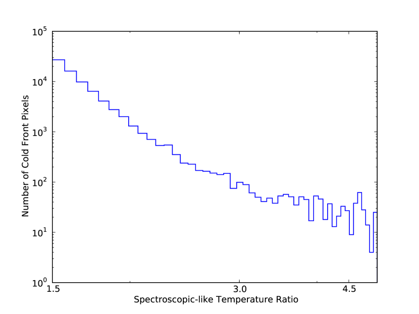
Figure 9.— Frequency of cold fronts as a function of ratio of $T_{sl}$ ratio from one side to the other identified in all cluster images (inside $r_{500}$) from 1.0$\geq z\geq$0.0.

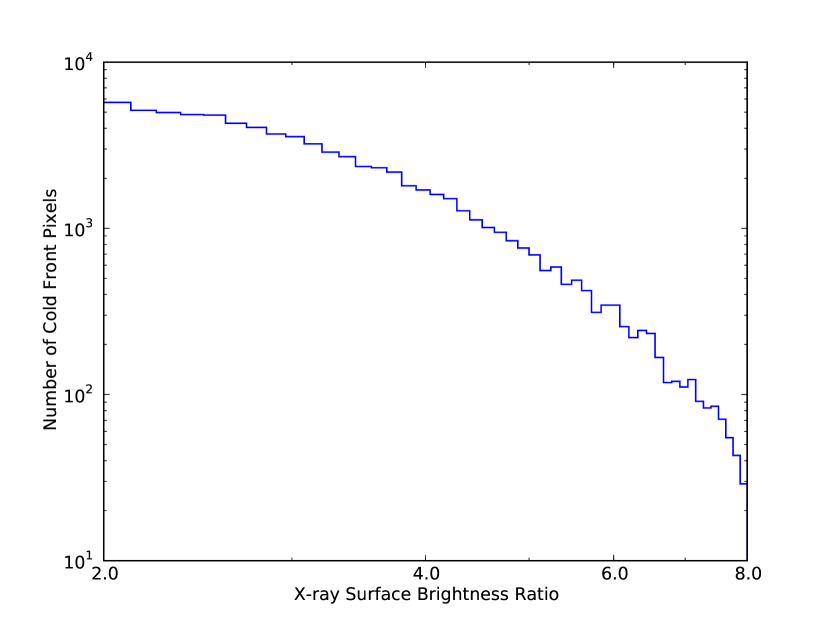
Figure 10.— Frequency of cold fronts as a function of ratio of 0.3-8.0 keV X-ray surface brightness from one side to the other in all simulated cluster projections (inside $r_{500}$ in the range 1.0$\geq z\geq$0.0.

Additionally, we can check the number of identified cold front pixels per simulated cluster image. We have already described this measurement as equivalent to the comoving total length ($L_{cf}$) of cold front features in the full image, though we make no effort here to determine if the features are contiguous. For now, this calculation gives us a sense of the total extent of cold fronts in all the simulated cluster images. Figure 11 shows the result of this calculation, a probability distribution function for the total comoving length of cold fronts in the synthetic cluster maps at three redshifts. Interestingly, the distributions at three redshifts (1.0, 0.5 and 0.0) overlap quite well. The normalization is adjusted by the total number of objects with cold fronts identified, but the relative number of objects with a specific measured length of cold fronts is more or less constant across redshift. The high $L_{cf}$ end of the distribution grows longer at later times, presumably because the objects progressively get larger, and therefore have larger values of $r_{500}$, thus more area within which to find cold fronts.

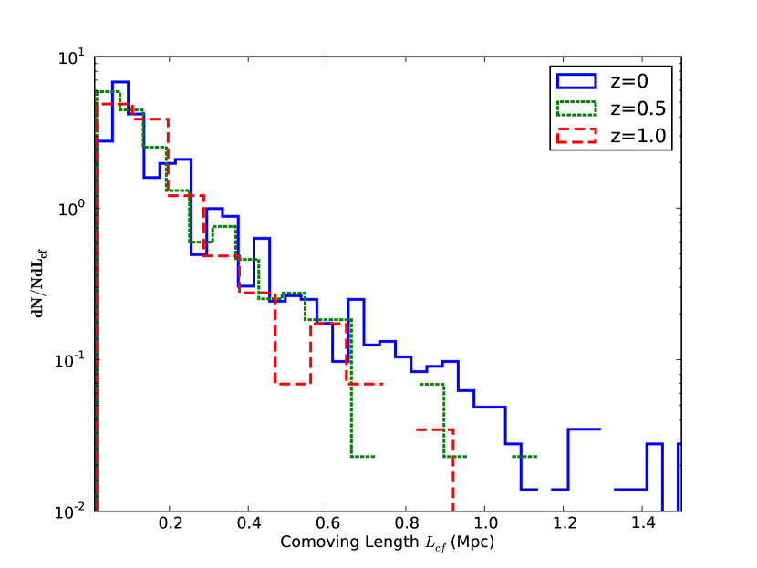
Figure 11.— Normalized probability distribution function for the comoving length of cold fronts ($L_{cf}$) in all cluster projections at 3 redshifts as indicated in the legend. The distribution of lengths is fairly constant with redshift, though the high $L_{cf}$ tail lengthens at lower redshift, due to the increased size of the largest clusters.

Since cold front jumps are observed to be continuous in pressure, we check, in projection, whether these features are consistent with observations. If we take the projected surface brightness jump and use it to estimate (roughly) the projected density jump, and compare that to the corresponding projected temperature jump, we can check to see if pressure continuity is met. The X-ray surface brightness in the 0.3-8.0 keV band is only very weakly dependent on temperature, and is effectively representative of the projected value of $n_{e}^{2}$. For one of our simulated cold front clusters, we show the properties of a cold front in Figure 12. We use the square root of the X-ray surface brightness jump as a proxy for the projected density, and multiply it by the value of $T_{sl}$ to form a projected pressure map. Figure 12 shows the obvious difference between the hot feature (a shock) and the cold feature behind it (a cold front). In the shock case, the jump in temperature corresponds to a pressure jump, and in the cold front case, the temperature jump is effectively continuous in pressure. Note also the opposite direction of the jump in surface brightness and temperature in the cold front. These jumps are typical of the shocks and cold fronts in the simulated clusters.

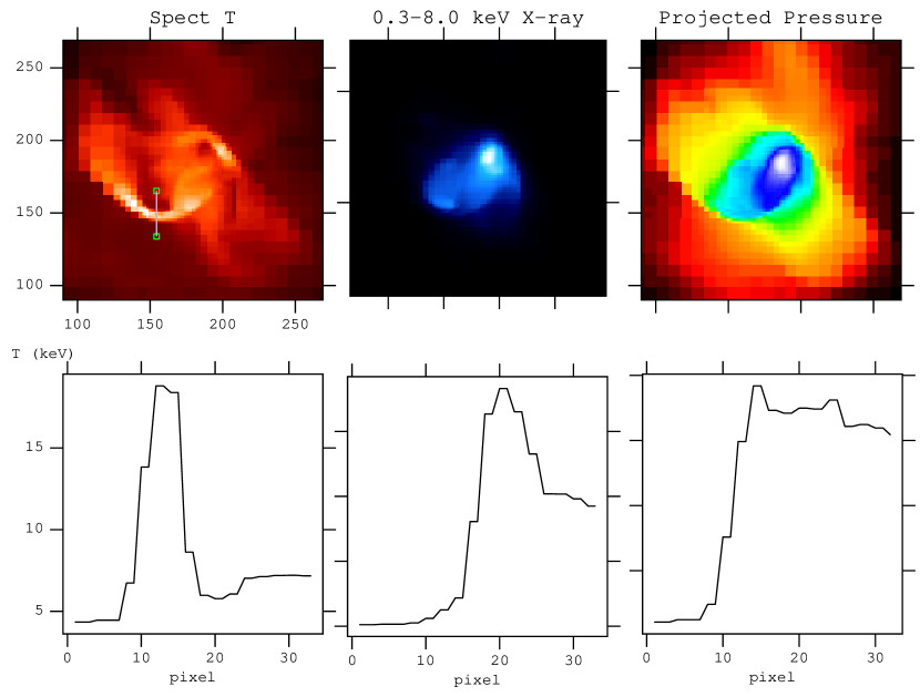
Figure 12.— Left to right: Projected images of $T_{sl}$, 0.3-8.0 keV X-ray surface brightness, and pressure for a cold front cluster with $M$ = 2$\times 10^{15}M_{\odot}$ at $z$=0 in the SFLC simulation. Also shown is the profile of $T_{sl}$, X-ray surface brightness and projected pressure across the shock and cold front in the lower panels. Location of the profile pixels is shown in the $T_{sl}$ image, where pixel zero is at the bottom of the line, and pixel 36 is at the top in the image. Pixel scale is 15.6h^-1kpc. Note the very hot shocked gas and the strong drop in temperature at the same location where the X-ray surface brightness goes up sharply behind the shock. Also note that at the shock, there is a strong pressure jump, while at the cold front (where the temperature drops and the surface brightness peaks) the pressure is roughly constant.

4.4. Cold Fronts in Individual Clusters

The cold fronts identified in the images of the simulated clusters have properties consistent with those observed in real galaxy clusters. The jumps in temperature are typically factors of 1.5-3, with a corresponding inverse change in the X-ray surface brightness, such that the features are continuous in pressure. Cold fronts in the simulated images are typically associated with shocks, as is clear in Figure 12. While we have not specifically looked at the observability of these features in the X-ray, it is clear from our data that the surface brightness in the hot shocked region is significantly lower than that in the cluster core. It is possible that many of these shocks would not be detected in X-rays for a typical exposure time, though the cold front would be more easily detectable. In future work, we will explore the statistics of cold fronts given the X-ray observability using more sophisticated synthetic observations including instrument response and X-ray backgrounds.

It is also worth exploring the recent history of the simulated clusters with the most obvious cold front features. Simulations show that cold fronts should be a good diagnostic for recent merger activity (e.g., Mathis et al., 2005; ZuHone & Markevitch, 2009), both in the case of sloshing type cold fronts and the more extended merger type cold fronts. A multipanel image of some of the most extended cold fronts in our simulated sample at $z$=0 are shown in Figure 13. The left column of this image shows the projected spectroscopic-like temperature (with identified cold fronts shown as white contours), and the right column is the X-ray surface brightness. In these cases it is very clear that the cold front finder has done a sufficiently accurate job of characterizing the cold front regions. We note that these cold fronts are all of the merger type, and not the sloshing type. We do not see the sloshing type cold fronts in these adiabatic clusters, and do not expect them given the lack of radiative cooling and steep central entropy gradients.

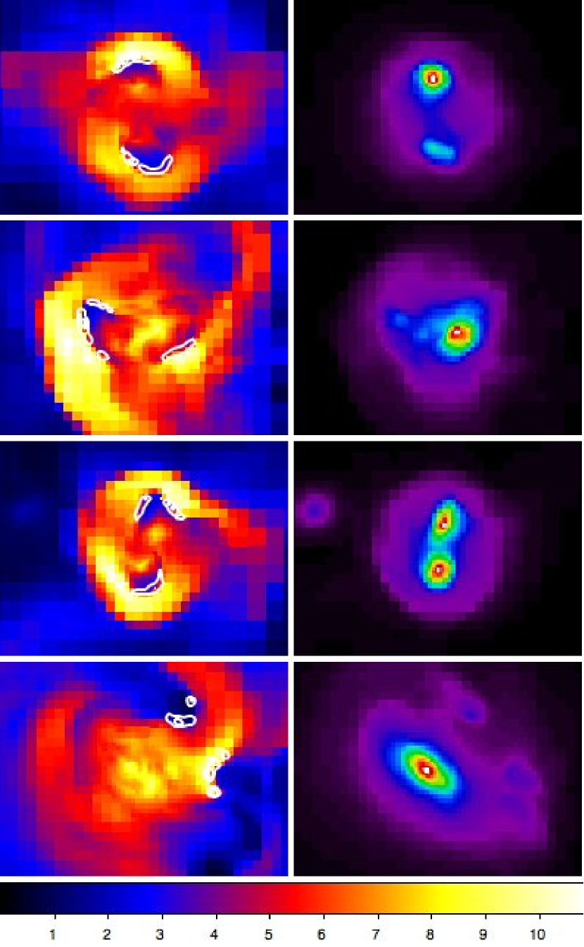
Figure 13.— Images of the simulated galaxy clusters with the most extended cold front structures. Left column is projected spectroscopic-like temperature with cold fronts identified using the automated method described in the text overlaid as white contours, second column is 0.3-8.0 keV X-ray surface brightness. Image scale is $\sim$3 Mpc. Colorbar indicates temperature scale from left column in keV. Masses of the clusters from top to bottom are: 1.4$\times 10^{15}M_{\odot}$, 8.5$\times 10^{14}M_{\odot}$, 4.8$\times 10^{14}M_{\odot}$, 1.98$\times 10^{15}M_{\odot}$.

For three of these obvious cold front clusters, we have taken snapshots of their recent history to illustrate the process by which these extended cold fronts are formed in the cosmological simulations. Recall that for this large set of simulated clusters, the physics in the simulation is purely adiabatic, meaning that there is no radiative cooling. Therefore any regions where cold and hot gas are in close proximity result either from shocks or adiabatic effects. The histories of these three clusters are shown in Figures 14,15 and 16. In each case, we see that the formation of the cold fronts is a result of a recent merger.

In Figures 14 and 16, we show two classic roughly plane-of-the-sky mergers, where in the earlier timesteps, the halos of the merger are clearly approaching each other, as evidenced by the shock features between them. At the later epoch, we see the subclusters after core passage, when the cold fronts have developed. We also show the dark matter contours, and there appears to be some mild separation of the dark matter centroids from the gas peaks, though we have not quantified this result in this work. In Figure 15, we see an array of cold fronts throughout the history of the cluster, but in this case the dynamics are more complicated. In the far left panels, we see a situation where there has been an initial core passage of two subclusters. The second panels show the approach of the two objects as they fall back together, with an obvious shock between, while at the same time a third subcluster approaches from the lower left. In the third panel, the initial merger has had a second core passage, while the extra merging subcluster is now driving a shock as it wraps around the subcluster in the upper left. At the final stage, there are two very obvious cold fronts, but deducing the merging history from the final snapshot could be quite challenging.

Cold fronts in the simulated clusters result from a variety of dynamical scenarios, ranging from simple binary mergers to multiple simultaneous mergers. The appearance of cold fronts and shocks is however a generic result of all kinds of mergers in these systems.

Figure 14.— Time sequence of development of a cold front in a 1.4$\times 10^{15}M_{\odot}$ cluster (same as the cluster in the top panels of Figure 13). Left panels are at $z$=0.1, right are at $z$=0. Upper panels show projected spectroscopic-like temperature in color and 0.3-8.0 keV X-ray surface brightness in contours. Color range in $T_{sl}$ goes from 3 keV (blue) to 10 keV (white). Bottom panel is X-ray surface brightness in color and projected dark matter density contours. Colorbar on this image shows range of X-ray surface brightness in $ergs/s/cm^{2}/pixel$ at the face of the projected simulation box (not corrected for distance of observer) to allow a comparison between the two images. Image scale is 2.0 Mpc. Note the obvious merger at $z$=0.1, which creates the cold fronts after the cores of the subclusters pass through each other.

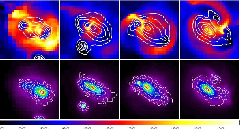
Figure 15.— Time sequence for a cold front developing in a 1.98 $\times 10^{15}M_{\odot}$ cluster (same as the cluster in the bottom panels of Figure 13). Left to right panels are forward in time, from $z$=0.3, $z$=0.2, $z$=0.1 and $z$=0.0. Upper and lower panels show the same quantities as in Figure 14. Image scale is 4.0 Mpc, colorbar is $T_{sl}$ in Kelvin for the upper panels. Note the obvious cold fronts in the earliest timestep, followed by a recollapse and shock, then an additional subgroup merges at the same time in the third timestep, causing the development of multiple cold fronts simultaneously.

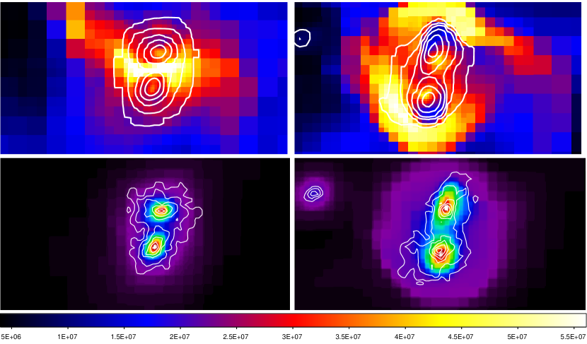
Figure 16.— Time sequence for a 4.8$\times 10^{14}M_{\odot}$ cluster (same as the cluster in the second from bottom panels of Figure 13), right panels are $z$=0, left are $z$=0.1. Image quantities are the same as Figures 14 and 15. Colorbar is $T_{sl}$ in Kelvin for the upper panels. Image scale is 2.0 Mpc. Note the similarities to Figure 14, with an obvious plane of the sky merger in the first timestep and the classic post core-crossing cold fronts in the second timestep.

4.5. Cold-Front Cluster Morphology

Figure 17.— Probability density function of clusters as a function of $P_{3}$/$P_{0}$ power ratio for each cluster image in the $z$=0 sample. Green dashed line is cold front clusters, blue solid line is non-cold front clusters. Cold front clusters are those that have a minimum comoving length of cold front pixels $L_{cf}>156h^{-1}$kpc comoving.

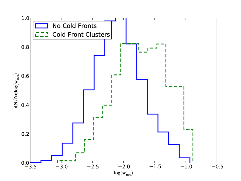
Figure 18.— Probability density function of clusters as a function of centroid shift for each cluster image in the $z$=0 sample. Green dashed line is cold front clusters, blue solid line is non-cold front clusters. Cold front clusters are those that have a minimum comoving length of cold front pixels $L_{cf}>156h^{-1}$kpc comoving.

Recent studies of well-known cold front clusters identify a possible relationship between the presence of X-ray cold fronts and the merger state of the clusters (Owers et al., 2009). There is also some indication that in some fraction of clusters the presence of the cold front may be the only indicator of a recent merger (Ghizzardi et al., 2010). To test these ideas, we have undertaken a study of the X-ray morphology of the clusters in our simulated samples via the measurement of power ratios and centroid shifts of the X-ray images. These quantitative measures are an indicator of whether the X-ray morphologies are obviously disturbed or regular, and are a proxy for deciding whether a cluster is dynamically active or relaxed (Jeltema et al., 2008; Ventimiglia et al., 2008).

In short, the power ratios are the multipole moments of the X-ray surface brightness map from a circular aperture centered on the cluster X-ray centroid (see Buote & Tsai, 1995, 1996; Jeltema et al., 2005). As described elsewhere, this method is related to the multipole expansion of the two-dimensional gravitational potential. This set of equations is reproduced from Jeltema et al. (2008). The multipole expansion of the two-dimensional gravitational potential is

$$\Psi(R,\phi)=-2Ga_{0}\ln\left({1\over R}\right)-2G\sum^{\infty}_{m=1}{1\over mR^{m}}$$

$$\left(a_{m}\cos m\phi+b_{m}\sin m\phi\right).$$ (12)

and the moments $a_{m}$ and $b_{m}$ are

$$a_{m}(R) = \int_{R^{\prime}\leq R}\Sigma(\vec{x}^{\prime})\left(R^{\prime}\right)^{m}\cos m\phi^{\prime}d^{2}x^{\prime},$$

$$b_{m}(R) = \int_{R^{\prime}\leq R}\Sigma(\vec{x}^{\prime})\left(R^{\prime}\right)^{m}\sin m\phi^{\prime}d^{2}x^{\prime},$$

where $\vec{x}^{\prime}=(R^{\prime},\phi^{\prime})$ and $\Sigma$ is the surface mass density. In the case of X-ray studies, X-ray surface brightness replaces surface mass density in the calculation of the power ratios.

The powers are formed by integrating the magnitude of $\Psi_{m}$, the mth term in the multipole expansion of the potential given in equation (12), over a circle of radius $R$,

$$P_{m}(R)={1\over 2\pi}\int^{2\pi}_{0}\Psi_{m}(R,\phi)\Psi_{m}(R,\phi)d\phi.$$ (13)

Ignoring factors of $2G$, this gives

$$P_{0}=\left[a_{0}\ln\left(R\right)\right]^{2}$$

$$P_{m}={1\over 2m^{2}R^{2m}}\left(a^{2}_{m}+b^{2}_{m}\right).$$

The higher multipole moments are sensitive to the amount of substructure in the cluster. In most cases, as in this work, we normalize the multipole moments $P_{2}$, $P_{3}$ and $P_{4}$ to $P_{0}$ to factor out the overall brightness of the cluster. $P_{2}$, the second multipole moment is sensitive to deviations from circularity, $P_{3}$ to deviations from mirror symmetry, and $P_{4}$ is similar to $P_{2}$, but sensitive to smaller scale asymmetry. Each of the moments has a component of radial decline in the cluster profile which contributes to its value, such that substructure at large radius leads to larger power ratios. Perfectly round clusters (irrespective of the shape of the radial profile) would give all zero power ratios. While each of the power ratios is sensitive to slightly different asymmetries, it is important to note that they are strongly correlated with one another. That means that clusters that are disturbed via merging activity typically show deviations from circularity, as well as from mirror symmetry and small scale substructure simultaneously. In this work, we use the values of the power ratios inside a radius of $r_{500}$, a radius which is typically observable in X-rays for a large set of galaxy clusters. We note that the value of the power ratio selected is somewhat dependent on the outer radius used, and that merging clusters with disturbances on larger scales than the outer radius may be missed when using $r_{500}$ (Takizawa et al., 2010).

A second type of quantitative measure we employ in this study is the centroid shift (see Mohr et al., 1993; O’Hara et al., 2006; Poole et al., 2006; Maughan, 2007). Centroids of the X-ray surface brightness are measured successively in apertures of increasing size. The centroid shift is the variation of the centroid with radius (see above references and Jeltema et al., 2008), and is an indicator of deviations from dynamical equilibrium. Our main interest here is in the change of the mean centroid shifts from the non-cold front clusters to the cold front clusters.

Table 1Median Power Ratios and Centroid Shifts

Measure	Cold Front Clusters	Non-Cold Front Clusters
$P_{2}$/$P_{0}$	1.75e-6	5.71e-7
$P_{3}$/$P_{0}$	2.25e-8	4.02e-9
$P_{4}$/$P_{0}$	6.50e-9	8.57e-10
Centroid Shift	0.0146	0.0080

We find that clusters identified as having cold fronts have systematically higher values for the power ratios and centroid shifts than those that do not have cold fronts. This result is statistically significant at $>99$% when a Kolmogorov-Smirnov test is applied. Table 1 shows the median values for the power ratios and centroid shifts for clusters identified as cold front clusters and those without cold fronts. Figures 17 and 18 show the distribution of $P_{3}$/$P_{0}$ and centroid shifts in the cluster sample for both cold front and non-cold front clusters in the sample at $z$=0. The other power ratios have very similar distributions.

This result holds for all clusters with even a single pixel identified as a cold front, but it becomes monotonically more significant when we increase the threshold for number of pixels identified as cold fronts. This measure is equivalent to total length of cold front features. Figure 19 shows a histogram of the $P_{3}$/$P_{0}$ power ratio for the clusters in samples with increasing numbers of cold front pixels. As we raise the threshold for number of pixels identified as cold fronts, the morphology becomes systematically more disturbed, as is expected if cold fronts are related to merging events. This trend is repeated in the other power ratios, as well as the centroid shift measure. In Figure 19, the number of cold front pixels identified in the $z$=0 simulated clusters increases as the distribution shifts to the more disturbed (right) side of the distribution. As noted in earlier sections, $L_{cf}$ can be thought of roughly as a total extent of cold front features, where in these images, the pixel scale is 15.6$h^{-1}$kpc.

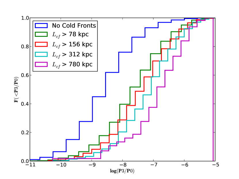
Figure 19.— Cumulative fraction of cluster images as a function of $P_{3}$/$P_{0}$ power ratio for clusters with increasing threshold for number of cold front pixels identified. Blue line represents all cluster images with no cold front pixels identified. Red line represents 5 identified pixels ($L_{cf}>78h^{-1}$kpc), green line is for 10 pixels ($L_{cf}>156h^{-1}$kpc), cyan line is for 20 pixels ($L_{cf}>312h^{-1}$kpc), purple line is for images with 50 or more cold front pixels ($L_{cf}>780h^{-1}$kpc). Note the shift in the median of the distribution to more disturbed (higher) $P_{3}$/$P_{0}$ values as the threshold for minimum number of cold front pixels is raised.

5. Effects of Baryonic Physics

Two other simulations are used to study the effect of additional non-gravitational physics on the properties of cold fronts. While not a convergence study, these results are presented to give a basic indication of the impact of additional baryonic physics on the result. We know observationally that in galaxy clusters the gas physics is not purely adiabatic. It is well-known that in the core regions of clusters, radiative cooling becomes important, in many clusters the estimated cooling times are significantly shorter than a Hubble time. In addition, there are both heat and metals injected from cluster galaxies due to star formation, and there is also strong evidence of AGN activity. In this case, we explore the result of including additional physical processes on the incidence of cold fronts in the simulated clusters.

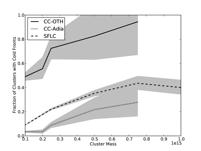
Figure 20.— Fraction of cluster projections hosting at least 10 pixels ($L_{cf}>156h^{-1}kpc$) identified by the automated cold front finder. Solid line is for the CC-OTH run described in the text, with radiative cooling and star formation plus feedback. Dashed line represents the SFLC simulation, and is replotted data from Figure 4. Dotted line is for the CC-Adia run, identical to CC-OTH, but with only adiabatic gas physics. Gray regions are 1$\sigma$ Poisson error bars.

Our main result is shown in Figure 20, showing the fraction of clusters with at least 10 cold front pixels (in this case the images have the same pixel scale across all simulations) as a function of cluster mass. The plot axes match Figure 4, and the result from that figure are overplotted with the same result from the CC-Adia and CC-OTH simulations. Several things are obvious in this comparison, the first is that these simulations probe different cluster mass ranges, since the SFLC represents a much larger physical volume than CC-Adia and CC-OTH. The second is that including radiative cooling and feedback results in significantly more clusters hosting cold fronts. This is not unexpected, as the cooling of cluster cores, as well as subclusters, results in more cold edges surrounded by hot gas. Figure 21 illustrates this effect, comparing the identical cluster in both the CC-Adia and CC-OTH runs.

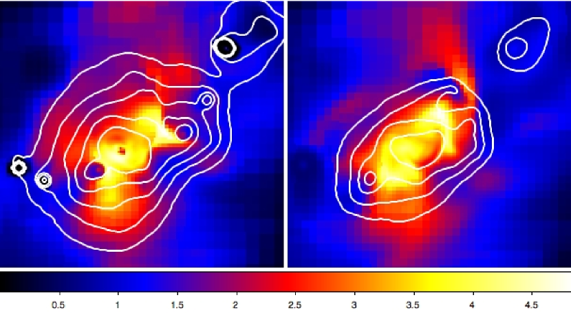
Figure 21.— Comparison of $T_{sl}$ maps for the same cluster in two different simulations, the left panel is from the simulation designated CC-OTH and the right is from CC-Adia. $T_{sl}$ is the image quantity, the contours are synthetic 0.3-8.0 keV X-ray surface brightness contours with the same limits in each map. The 6.1$\times 10^{14}M_{\odot}$ cluster from the CC-OTH (simulation with radiative cooling, star formation and thermal/metal feedback) in the left panel, and the same cluster in the adiabatic simulation is shown in the right panel. Image scale is roughly 3$h^{-1}$Mpc square for each panel. Note the significant difference in the temperature maps, with the cold subclumps very obvious in the CC-OTH cluster map. Note that the cold subclumps create peaks in the X-ray contours.

Figure 22 shows the trending of fraction of cold front clusters with redshift in our simulation with additional baryonic physics (CC-OTH). While the fraction has some variation with redshift, within the statistical errors of the sample the trend is roughly flat. This compares well with the SFLC adiabatic run, though there is a mild increase in the fraction of cold front clusters from high to low redshift in that simulation. In CC-OTH, the fraction goes from roughly 0.64 at $z$=0.9 to 0.54 at $z$=0. However, as noted, the Poisson errors are large ($\sim\pm$0.1 at all $z$) due to the smaller cluster sample in this simulation.

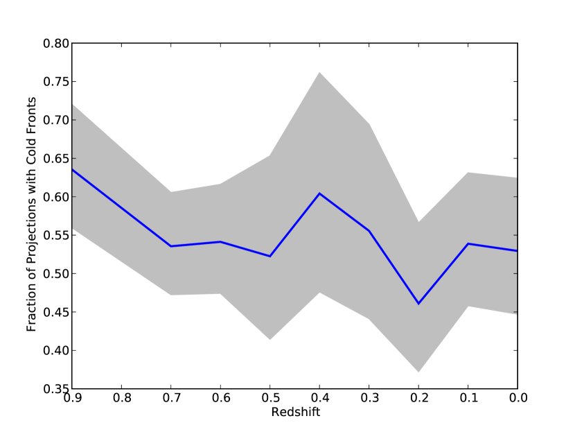
Figure 22.— Fraction of clusters with M$\geq 10^{14}$ in the CC-OTH simulation with cold front length $L_{cf}>156h^{-1}kpc$ as a function of redshift. Gray region is 1$\sigma$ Poisson error bars.

Additionally we can compare the fraction of clusters with cold fronts from SFLC to CC-Adia, since the physics is identical, though the mass resolution is different. CC-Adia has a lower incidence of cold front clusters than does SFLC, which is somewhat surprising. However, given the number of changes between SFLC and CC-Adia, it is premature to make strong conclusions. For example the much reduced box size in our smaller simulations (from 512$h^{-1}$Mpc to 128$h^{-1}$Mpc cubic volume) leads to a radical reduction in large-scale power in the simulation box. What has not changed between any of these runs, however, is the increasing trend of fraction of cold front clusters with mass.

6. Discussion and Summary

We have shown the incidence of X-ray cold fronts in a large sample of simulated galaxy clusters. In this initial study, to maximize the number of clusters in the sample at useful grid resolution, we gather the statistical results from an adiabatic simulation. We identify cold fronts using projected maps of spectroscopic-like temperature ($T_{sl}$ ), and X-ray surface brightness generated with Cloudy. We show the effect of additional baryonic physics using two smaller volume simulations, identical in initial conditions, one using adiabatic physics, and the other including the effects of radiative cooling, star formation and metal/thermal feedback. The main results are summarized here.

• The trends of simulated galaxy clusters with cold front features with redshift depends significantly on cluster selection. When using a mass-limited sample the trend out to $z$=1.0 is weak, irrespective of the threshold of number of identified cold front pixels. This weak trending occurs only when the sample is mass-limited, however. When limiting the sample by the rarity of peaks using a constant $\sigma_{M}$, the incidence of cold fronts shows a decreasing trend with redshift, and when using a flux limit derived from X-ray scaling relations, the trend is increasing with redshift.

• There is in the simulated cold front clusters a strong trend with cluster mass, the more massive clusters being much more likely to host a cold front. In the adiabatic sample, the fraction of clusters hosting cold fronts with $L_{cf}>156h^{-1}kpc$ with M$>7.5\times 10^{14}M_{\odot}$ is 40-50% depending on the redshift of the sample. In the simulation with radiative cooling, star formation and thermal feedback, that fraction can be higher than 80% at the high mass end.

• The fraction of clusters hosting cold fronts in the adiabatic simulations is lower than in observed samples, which give fractions anywhere from 40-80% depending on the sample and the redshift coverage. We know given our method that we probably underestimate the total number of cold fronts, so this is not surprising. In our flux-limited sample from the simulations, we find 15% of cluster with $L_{cf}>156h^{-1}$kpc. We show that including radiative cooling and star formation in the simulations will increase this fraction significantly without changing the general trends with mass and redshift. Additionally as noted above, the highest mass clusters in our sample show a higher cold front fraction, around 40-50%.

• Cold fronts in simulated clusters are almost universally the result of mergers of various sizes, and are almost always associated with shocks. This result is still qualitative, but we hope to make more quantitative claims in subsequent work.

• The association of cold front clusters with mergers is confirmed in a statistical sense using the quantitative morphological measures for the X-ray surface brightness maps. Clusters with cold fronts are preferentially more disturbed when measured using power ratios and centroid shifts. The significance of this result increases if we select clusters with higher numbers of identified cold front pixels.

• There is a clear impact on the incidence of cold fronts due to changes in baryonic physics of the simulation. When including radiative cooling and star formation and feedback to the simulations, the incidence of cold fronts goes up strongly to greater than 50% of clusters at all masses. While the normalization of the number of cold fronts in simulated clusters is strongly affected by the baryonic physics, the trending with mass and redshift is not.

The most obvious improvements that can be made to this analysis are a full resolution and convergence study with variations in baryonic physics, and an analysis of the statistics of cold fronts expected with more realistic X-ray images and temperature maps including X-ray instrumental effects and backgrounds.

Since it is clear from our analysis of the additional small box simulations that our results depend on box size and baryonic physics, the first step is most obvious. However, the statistics of the cold front clusters are only useful if they can be related to observational results. The effect of the length of exposure, redshift of the cluster, angular size of the cluster in relation to the chip size and spatial response, and the spectral response all will play a role in detectability of these features.

In addition, our result regarding the redshift trends of cold front clusters is clearly a result of sample selection. What the “right” sample selection should be is unclear, but for observational comparison, it is appropriate to use flux-limited samples. We believe the result on the incidence as a function of mass to be robust at this point, since the two additional simulations show the same trend, though with differing normalization. Finally, further study can illuminate how cold fronts can be used as a diagnostic of recent merger history. A full study of how the properties of the cold fronts in any given cluster can be used to deduce recent merger history will also be the topic of future work.

References

- Asai et al. (2004) Asai, N., Fukuda, N., & Matsumoto, R. 2004, ApJ, 606, L105
- Asai et al. (2007) —. 2007, ApJ, 663, 816
- Ascasibar & Markevitch (2006) Ascasibar, Y. & Markevitch, M. 2006, ApJ, 650, 102
- Berger & Colella (1989) Berger, M. J. & Colella, P. 1989, J. Comp. Phys., 82, 64
- Bialek et al. (2002) Bialek, J. J., Evrard, A. E., & Mohr, J. J. 2002, ApJ, 578, L9
- Birnboim et al. (2009) Birnboim, Y., Keshet, U., & Hernquist, L. 2009, ArXiv 0912.2094
- Böhringer et al. (2001) Böhringer, H., Schuecker, P., Guzzo, L., Collins, C. A., Voges, W., Schindler, S., Neumann, D. M., Cruddace, R. G., De Grandi, S., Chincarini, G., Edge, A. C., MacGillivray, H. T., & Shaver, P. 2001, A&A, 369, 826
- Bryan & Norman (1997a) Bryan, G. & Norman, M. 1997a, 12th Kingston Meeting on Theoretical Astrophysics, proceedings of meeting held in Halifax; Nova Scotia; Canada October 17-19; 1996 (ASP Conference Series # 123), ed. D. Clarke. & M. Fall
- Bryan & Norman (1997b) —. 1997b, Workshop on Structured Adaptive Mesh Refinement Grid Methods, ed. N. Chrisochoides (IMA Volumes in Mathematics No. 117)
- Buote & Tsai (1995) Buote, D. A. & Tsai, J. C. 1995, ApJ, 452, 522
- Buote & Tsai (1996) —. 1996, ApJ, 458, 27
- Carroll et al. (1992) Carroll, S. M., Press, W. H., & Turner, E. L. 1992, ARA&A, 30, 499
- Cen & Ostriker (1999) Cen, R. & Ostriker, J. P. 1999, ApJ, 514, 1
- Dupke & White (2003) Dupke, R. & White, III, R. E. 2003, ApJ, 583, L13
- Efstathiou et al. (1985) Efstathiou, G., Davis, M., White, S. D. M., & Frenk, C. S. 1985, ApJS, 57, 241
- Eisenstein & Hu (1999) Eisenstein, D. J. & Hu, W. 1999, ApJ, 511, 5
- Eisenstein & Hut (1998) Eisenstein, D. J. & Hut, P. 1998, ApJ, 498, 137
- Ettori & Fabian (2000) Ettori, S. & Fabian, A. C. 2000, MNRAS, 317, L57
- Ferland et al. (1998) Ferland, G. J., Korista, K. T., Verner, D. A., Ferguson, J. W., Kingdon, J. B., & Verner, E. M. 1998, PASP, 110, 761
- Ghizzardi et al. (2006) Ghizzardi, S., Molendi, S., Leccardi, A., & Rossetti, M. 2006, in ESA Special Publication, Vol. 604, The X-ray Universe 2005, ed. A. Wilson, 717–+
- Ghizzardi et al. (2010) Ghizzardi, S., Rossetti, M., & Molendi, S. 2010, ArXiv 1003.1051
- Haardt & Madau (1996) Haardt, F. & Madau, P. 1996, ApJ, 461, 20
- Hallman & Markevitch (2004) Hallman, E. J. & Markevitch, M. 2004, ApJ, 610, L81
- Hallman et al. (2007) Hallman, E. J., O’Shea, B. W., Burns, J. O., Norman, M. L., Harkness, R., & Wagner, R. 2007, ApJ, 671, 27
- Hallman et al. (2009) Hallman, E. J., O’Shea, B. W., Smith, B. D., Burns, J. O., & Norman, M. L. 2009, ApJ, 698, 1795
- Hart et al. (2009) Hart, Q. N., Stocke, J. T., & Hallman, E. J. 2009, ApJ, 705, 854
- Heinz et al. (2003) Heinz, S., Churazov, E., Forman, W., Jones, C., & Briel, U. G. 2003, MNRAS, 346, 13
- Hockney & Eastwood (1988) Hockney, R. W. & Eastwood, J. W. 1988, Computer Simulation Using Particles (Institute of Physics Publishing)
- Jeltema et al. (2005) Jeltema, T. E., Canizares, C. R., Bautz, M. W., & Buote, D. A. 2005, ApJ, 624, 606
- Jeltema et al. (2008) Jeltema, T. E., Hallman, E. J., Burns, J. O., & Motl, P. M. 2008, ApJ, 681, 167
- Jenkins et al. (2001) Jenkins, A., Frenk, C. S., White, S. D. M., Colberg, J. M., Cole, S., Evrard, A. E., Couchman, H. M. P., & Yoshida, N. 2001, MNRAS, 321, 372
- Johnson et al. (2010) Johnson, R. E., Markevitch, M., Wegner, G. A., Jones, C., & Forman, W. R. 2010, ApJ, 710, 1776
- Keshet et al. (2009) Keshet, U., Markevitch, M., Birnboim, Y., & Loeb, A. 2009, ArXiv 0912.3526
- Lyutikov (2006) Lyutikov, M. 2006, MNRAS, 373, 73
- Mantz et al. (2009) Mantz, A., Allen, S. W., Ebeling, H. andRapetti, D., & Drlica-Wagner, A. 2009, ArXiv e-prints, 0909.3099
- Markevitch et al. (2002) Markevitch, M., Gonzalez, A. H., David, L., Vikhlinin, A., Murray, S., Forman, W., Jones, C., & Tucker, W. 2002, ApJ, 567, L27
- Markevitch et al. (2000) Markevitch, M., Ponman, T. J., Nulsen, P. E. J., Bautz, M. W., Burke, D. J., David, L. P., Davis, D., Donnelly, R. H., Forman, W. R., Jones, C., Kaastra, J., Kellogg, E., Kim, D., Kolodziejczak, J., Mazzotta, P., Pagliaro, A., Patel, S., Van Speybroeck, L., Vikhlinin, A., Vrtilek, J., Wise, M., & Zhao, P. 2000, ApJ, 541, 542
- Markevitch & Vikhlinin (2007) Markevitch, M. & Vikhlinin, A. 2007, Phys. Rep., 443, 1
- Markevitch et al. (2003) Markevitch, M., Vikhlinin, A., & Forman, W. R. 2003, in Astronomical Society of the Pacific Conference Series, Vol. 301, Astronomical Society of the Pacific Conference Series, ed. S. Bowyer & C.-Y. Hwang, 37–+
- Markevitch et al. (2001) Markevitch, M., Vikhlinin, A., & Mazzotta, P. 2001, ApJ, 562, L153
- Mastropietro & Burkert (2008) Mastropietro, C. & Burkert, A. 2008, MNRAS, 389, 967
- Mathis et al. (2005) Mathis, H., Lavaux, G., Diego, J. M., & Silk, J. 2005, MNRAS, 357, 801
- Maughan (2007) Maughan, B. J. 2007, ApJ, 668, 772
- Mazzotta et al. (2001) Mazzotta, P., Markevitch, M., Vikhlinin, A., Forman, W. R., David, L. P., & van Speybroeck, L. 2001, ApJ, 555, 205
- Mazzotta et al. (2004) Mazzotta, P., Rasia, E., Moscardini, L., & Tormen, G. 2004, MNRAS, 354, 10
- Mohr et al. (1993) Mohr, J. J., Fabricant, D. G., & Geller, M. J. 1993, ApJ, 413, 492
- Nagai & Kravtsov (2003) Nagai, D. & Kravtsov, A. V. 2003, ApJ, 587, 514
- Norman & Bryan (1999) Norman, M. & Bryan, G. 1999, Numerical Astrophysics : Proceedings of the International Conference on Numerical Astrophysics 1998 (NAP98), held at the National Olympic Memorial Youth Center, Tokyo, Japan, March 10-13, 1998., ed. K. T. S. M. Miyama & T. Hanawa (Kluwer Academic)
- O’Hara et al. (2006) O’Hara, T. B., Mohr, J. J., Bialek, J. J., & Evrard, A. E. 2006, ApJ, 639, 64
- O’Shea et al. (2004) O’Shea, B., Bryan, G., Bordner, J., Norman, M., Abel, T., & Harkness, R. amd Kritsuk, A. 2004, Adaptive Mesh Refinement - Theory and Applications, ed. T. Plewa, T. Linde, & G. Weirs (Springer-Verlag)
- O’Shea et al. (2005) O’Shea, B. W., Nagamine, K., Springel, V., Hernquist, L., & Norman, M. L. 2005, ApJS, 160, 1
- Owers et al. (2009) Owers, M. S., Nulsen, P. E. J., Couch, W. J., & Markevitch, M. 2009, ApJ, 704, 1349
- Poole et al. (2006) Poole, G. B., Fardal, M. A., Babul, A., McCarthy, I. G., Quinn, T., & Wadsley, J. 2006, MNRAS, 373, 881
- Press & Schechter (1974) Press, W. H. & Schechter, P. 1974, ApJ, 187, 425
- Rasia et al. (2005) Rasia, E., Mazzotta, P., Borgani, S., Moscardini, L., Dolag, K., Tormen, G., Diaferio, A., & Murante, G. 2005, ApJ, 618, L1
- Roettiger et al. (1999) Roettiger, K., Burns, J. O., & Stone, J. M. 1999, ApJ, 518, 603
- Ryu et al. (2003) Ryu, D., Kang, H., Hallman, E., & Jones, T. W. 2003, ApJ, 593, 599
- Skillman et al. (2008) Skillman, S. W., O’Shea, B. W., Hallman, E. J., Burns, J. O., & Norman, M. L. 2008, ApJ, 689, 1063
- Smith et al. (2008) Smith, B., Sigurdsson, S., & Abel, T. 2008, MNRAS, 385, 1443
- Smith et al. (2010) Smith, B. D., Hallman, E. J., Shull, J. M., & O’Shea, B. W. 2010, ArXiv 1009.0261
- Springel & Farrar (2007) Springel, V. & Farrar, G. R. 2007, MNRAS, 380, 911
- Takizawa (2005) Takizawa, M. 2005, ApJ, 629, 791
- Takizawa (2008) —. 2008, ApJ, 687, 951
- Takizawa et al. (2010) Takizawa, M., Nagino, R., & Matsushita, K. 2010, PASJ, 62, 951
- Tittley & Henriksen (2005) Tittley, E. R. & Henriksen, M. 2005, ApJ, 618, 227
- Ventimiglia et al. (2008) Ventimiglia, D. A., Voit, G. M., Donahue, M., & Ameglio, S. 2008, ApJ, 685, 118
- Vikhlinin et al. (2001a) Vikhlinin, A., Markevitch, M., & Murray, S. S. 2001a, ApJ, 551, 160
- Vikhlinin et al. (2001b) —. 2001b, ApJ, 549, L47
- ZuHone & Markevitch (2009) ZuHone, J. A. & Markevitch, M. 2009, ArXiv 0909.0560