Efficient Interpolant Generation
in Satisfiability Modulo Linear Integer Arithmetic

Abstract.

The problem of computing Craig interpolants in SAT and SMT has recently received a lot of interest, mainly for its applications in formal verification. Efficient algorithms for interpolant generation have been presented for some theories of interest —including that of equality and uninterpreted functions ($\mathcal{EUF}$), linear arithmetic over the rationals ($\mathcal{LA}(\mathbb{Q})$), and their combination— and they are successfully used within model checking tools. For the theory of linear arithmetic over the integers ($\mathcal{LA}(\mathbb{Z})$), however, the problem of finding an interpolant is more challenging, and the task of developing efficient interpolant generators for the full theory $\mathcal{LA}(\mathbb{Z})$ is still the objective of ongoing research.

In this article we try to close this gap. We build on previous work and present a novel interpolation algorithm for SMT($\mathcal{LA}(\mathbb{Z})$), which exploits the full power of current state-of-the-art SMT($\mathcal{LA}(\mathbb{Z})$) solvers. We demonstrate the potential of our approach with an extensive experimental evaluation of our implementation of the proposed algorithm in the MathSAT SMT solver.

1. Introduction

Given two formulas $A$ and $B$ such that $A\wedge B$ is inconsistent, a Craig interpolant (simply “interpolant” hereafter) for $(A,B)$ is a formula $I$ s.t. $A$ entails $I$, $I\wedge B$ is inconsistent, and all uninterpreted symbols of $I$ occur in both $A$ and $B$.

Interpolation in both SAT and SMT has been recognized to be a substantial tool for formal verification. For instance, in the context of software model checking based on counter-example-guided-abstraction-refinement (CEGAR) interpolants of quantifier-free formulas in suitable theories are computed for automatically refining abstractions in order to rule out spurious counterexamples. Consequently, the problem of computing interpolants in SMT has received a lot of interest in the last years (e.g., [McM05, RSS10, YM05, KMZ06, CGS10, JCG08, LT08, FGG⁺09, GKT09, BKRW10, KLR10]). In the recent years, efficient algorithms and tools for interpolant generation for quantifier-free formulas in SMT have been presented for some theories of interest, including that of equality and uninterpreted functions ($\mathcal{EUF}$) [McM05, FGG⁺09], linear arithmetic over the rationals ($\mathcal{LA}(\mathbb{Q})$) [McM05, RSS10, CGS10], fixed-width bit-vectors [KW07, Gri11], and for combined theories [YM05, RSS10, CGS10, GKT09], and they are successfully used within model-checking tools.

For the theory of linear arithmetic over the integers ($\mathcal{LA}(\mathbb{Z})$), however, the problem of finding an interpolant is more challenging. In fact, it is not always possible to obtain quantifier-free interpolants starting from quantifier-free input formulas in the standard signature of $\mathcal{LA}(\mathbb{Z})$ (consisting of Boolean connectives, integer constants and the symbols $+,\cdot,\leq,=$) [McM05]. For instance, there is no quantifier-free interpolant for the $\mathcal{LA}(\mathbb{Z})$-formulas $A\stackrel{{\scriptstyle\text{\tiny def}}}{{=}}(2x-y+1=0)$ and $B\stackrel{{\scriptstyle\text{\tiny def}}}{{=}}(y-2z=0)$.

In order to overcome this problem, different research directions have been explored. One is to restrict to important fragments of $\mathcal{LA}(\mathbb{Z})$ where the problem does not occur. To this extent, efficient interpolation algorithms for the Difference Logic ($\mathcal{DL}$) and Unit-Two-Variables-Per-Inequality ($\mathcal{UTVPI}$) fragments of $\mathcal{LA}(\mathbb{Z})$ have been proposed in [CGS10]. Another direction is to extend the signature of $\mathcal{LA}(\mathbb{Z})$ to contain modular equalities $=_{c}$ (or, equivalently, divisibility predicates), so that it is possible to compute quantifier-free $\mathcal{LA}(\mathbb{Z})$ interpolants by means of quantifier elimination —which is however prohibitively expensive in general, both in theory and in practice. For instance, $I\stackrel{{\scriptstyle\text{\tiny def}}}{{=}}(-y+1=_{2}0)\equiv\exists x.(2x-y+1=0)$ is an interpolant for the formulas $(A,B)$ above. Using modular equalities, Jain et al. [JCG08] developed polynomial-time interpolation algorithms for linear equations and their negation and for linear modular equations. A similar algorithm was also proposed in [LT08]. The work in [BKRW10] was the first to present an interpolation algorithm for the full $\mathcal{LA}(\mathbb{Z})$ (augmented with divisibility predicates) which was not based on quantifier elimination. Finally, an alternative algorithm, exploiting efficient interpolation procedures for $\mathcal{LA}(\mathbb{Q})$ and for linear equations in $\mathcal{LA}(\mathbb{Z})$, has been presented in [KLR10].

The obvious limitation of the first research direction is that it does not cover the full $\mathcal{LA}(\mathbb{Z})$. For the second direction, the approaches so far seem to suffer from some drawbacks. In particular, some of the interpolation rules of [BKRW10] might result in an exponential blow-up in the size of the interpolants wrt. the size of the proofs of unsatisfiability from which they are generated. The algorithm of [KLR10] avoids this, but at the cost of significantly restricting the heuristics commonly used in state-of-the-art SMT solvers for $\mathcal{LA}(\mathbb{Z})$ (e.g. in the framework of [KLR10] both the use of Gomory cuts [Sch86] and of “cuts from proofs” [DDA09] is not allowed). More in general, the important issue of how to efficiently integrate the presented techniques into a state-of-the-art $\text{SMT}(\mathcal{LA}(\mathbb{Z}))$ solver is not immediate to foresee from the papers.

In this article we try to close this gap. After recalling the necessary background knowledge (§2), we present our contribution, which is twofold.

First (§3) we show how to extend the state-of-the art $\mathcal{LA}(\mathbb{Z})$-solver of MathSAT [Gri12] in order to implement interpolant generation on top of it without affecting its efficiency. To this extent, we combine different algorithms corresponding to the different submodules of the $\mathcal{LA}(\mathbb{Z})$-solver, so that each of the submodules requires only minor modifications, and implement them in MathSAT (MathSAT-modEq hereafter). An extensive empirical evaluation (§5) shows that MathSAT-modEq outperforms in efficiency all existing interpolant generators for $\mathcal{LA}(\mathbb{Z})$.

Second (§4), we propose a novel and general interpolation algorithm for $\mathcal{LA}(\mathbb{Z})$, independent from the architecture of MathSAT, which overcomes the drawbacks of the current approaches. The key idea is to extend both the signature and the domain of $\mathcal{LA}(\mathbb{Z})$: we extend the signature by adding the ceiling function $\lceil\cdot\rceil$ to it, and the domain by allowing non-variable terms to be non-integers. This greatly simplifies the interpolation procedure, and allows for producing interpolants which are much more compact than those generated by the algorithm of [BKRW10]. Also this novel technique was easily implemented on top of the $\mathcal{LA}(\mathbb{Z})$-solver of MathSAT without affecting its efficiency. (We call this implementation MathSAT-ceil.) An extensive empirical evaluation (§5) shows that MathSAT-ceil drastically outperforms MathSAT-modEq, and hence all other existing interpolant generators for $\mathcal{LA}(\mathbb{Z})$, for both efficiency and size of the final interpolant.

Finally, in §6 we report some related work, and in §7 we present some conclusions. We recall that a shorter version of this article appeared at TACAS 2011 conference [GLS11].

2. Background: $\text{SMT}(\mathcal{LA}(\mathbb{Z}))$

We first provide the necessary background. We will use the following notational conventions: $\bullet$

We denote formulas with $A$, $B$, $S$, $I$, $\varphi$, $\Gamma$.

Given a formula $\varphi$ partitioned into $A$ and $B$, the variables in $\varphi$ are denoted with $x$, $y$, $z$, $s$, $v$, $x_{i}$, $y_{j}$, $z_{k}$, $s_{h}$, $v_{l}$: $-$

$x_{i}$ for variables that occur only in $A$ ($A$-local);

$z_{k}$ for variables that occur only in $B$ ($B$-local);

$y_{j}$ for variables that occur both in $A$ and in $B$ ($AB$-common);

$v_{l}$ when we don’t want to distinguish them as in the above cases.

We denote integer constants with $a,b,c,d$.

We denote terms with $t_{1},t_{2}$. We write $t_{1}\cong t_{2}$ to denote that the two terms are syntactically identical, and $t_{1}=_{c}t_{2}$ to denote that they are congruent modulo $c$. With $\varphi_{1}\equiv\varphi_{2}$ we denote the logical equivalence of the two formulas $\varphi_{1}$ and $\varphi_{2}$.

We write $t\preceq A$ to denote that all the uninterpreted symbols occurring in $t$ occur also in $A$. In this case, we say that $t$ is $A$-pure. Given two formulas $A,B$ such that $t\preceq(A\cup B)$ but $t\not\preceq A$ and $t\not\preceq B$, we say that $t$ is $AB$-mixed.

2.1. Generalities

In this section we provide some background on SMT (§2.1.1) and on interpolation in SMT (§2.1.2).

2.1.1. Satisfiability Modulo Theory – SMT

Our setting is standard first order logic. We use the standard notions of theory, satisfiability, validity, logical consequence. A $0$-ary function symbol is called a constant. A term is a first-order term built out of function symbols and variables. If $t_{1},\ldots,t_{n}$ are terms and $p$ is a predicate symbol, then $p(t_{1},\ldots,t_{n})$ is an atom. A literal is either an atom or its negation. A formula $\phi$ is built in the usual way out of the universal and existential quantifiers, Boolean connectives, and atoms. We call a formula quantifier-free if it does not contain quantifiers, and ground if it does not contain free variables. A clause is a disjunction of literals. A formula is said to be in conjunctive normal form (CNF) if it is a conjunction of clauses. For every non-CNF $\mathcal{T}$-formula $\varphi$, an equisatisfiable CNF formula $\psi$ can be generated in polynomial time [Tse68].

We call Satisfiability Modulo (the) Theory $\mathcal{T}$, $\text{SMT}(\mathcal{T})$, the problem of deciding the satisfiability of quantifier-free formulas wrt. a background theory $\mathcal{T}$. Given a theory $\mathcal{T}$, we write $\phi\models_{\mathcal{T}}\psi$ (or simply $\phi\models\psi$) to denote that the formula $\psi$ is a logical consequence of $\phi$ in the theory $\mathcal{T}$. With $\phi\preceq\psi$ we denote that all uninterpreted (in $\mathcal{T}$) symbols of $\phi$ appear in $\psi$. If $C$ is a clause, $C\downarrow B$ is the clause obtained by removing all the literals whose atoms do not occur in $B$, and $C\setminus B$ that obtained by removing all the literals whose atoms do occur in $B$. With a little abuse of notation, we might sometimes denote conjunctions of literals $l_{1}\wedge\ldots\wedge l_{n}$ as sets $\{l_{1},\ldots,l_{n}\}$ and vice versa. If $\eta$ is the set $\{l_{1},\ldots,l_{n}\}$, we might write $\neg\eta$ to mean $\neg l_{1}\vee\ldots\vee\neg l_{n}$.

We call $\mathcal{T}$-solver a procedure that decides the consistency of a conjunction of literals in $\mathcal{T}$. If $S$ is a set of literals in $\mathcal{T}$, we call $\mathcal{T}$-conflict set w.r.t. $S$ any subset $\eta$ of $S$ which is inconsistent in $\mathcal{T}$. We call $\neg\eta$ a $\mathcal{T}$-lemma (notice that $\neg\eta$ is a $\mathcal{T}$-valid clause).

A standard technique for solving the SMT($\mathcal{T}$) problem is to integrate a DPLL-based SAT solver and a $\mathcal{T}$-solver in a lazy manner (see, e.g., [BSST09] for a detailed description). DPLL is used as an enumerator of truth assignments for the propositional abstraction of the input formula. At each step, the set of $\mathcal{T}$-literals in the current assignment is sent to the $\mathcal{T}$-solver to be checked for consistency in $\mathcal{T}$. If $S$ is inconsistent, the $\mathcal{T}$-solver returns a conflict set $\eta$, and the corresponding $\mathcal{T}$-lemma $\neg\eta$ is added as a blocking clause in DPLL, and used to drive the backjumping and learning mechanism.

[Resolution proof] Given a set of clauses $S\stackrel{{\scriptstyle\text{\tiny def}}}{{=}}\{C_{1},\ldots,C_{n}\}$ and a clause $C$, we call a resolution proof of the deduction $\bigwedge_{i}C_{i}\models_{\mathcal{T}}C$ a DAG ${\mathcal{P}}$ such that:

1. $C$ is the root of ${\mathcal{P}}$;

2. the leaves of ${\mathcal{P}}$ are either elements of $S$ or $\mathcal{T}$-lemmas;

3. each non-leaf node $C^{\prime}$ has two premises $C_{p_{1}}$ and $C_{p_{2}}$ such that $C_{p_{1}}\stackrel{{\scriptstyle\text{\tiny def}}}{{=}}p\vee\phi_{1}$, $C_{p_{2}}\stackrel{{\scriptstyle\text{\tiny def}}}{{=}}\neg p\vee\phi_{2}$, and $C^{\prime}\stackrel{{\scriptstyle\text{\tiny def}}}{{=}}\phi_{1}\vee\phi_{2}$. The atom $p$ is called the pivot of $C_{p_{1}}$ and $C_{p_{2}}$.

If $C$ is the empty clause (denoted with $\bot$), then ${\mathcal{P}}$ is a resolution proof of ($\mathcal{T}$-)unsatisfiability for $\bigwedge_{i}C_{i}$.

2.1.2. Interpolation in SMT

We consider the $\text{SMT}(\mathcal{T})$ problem for some background theory $\mathcal{T}$. Given an ordered pair $(A,B)$ of formulas such that $A\wedge B\models_{\mathcal{T}}\bot$, a Craig interpolant (simply “interpolant” hereafter) is a formula $I$ s.t.

1. $A\models_{\mathcal{T}}I$,

2. $I\land B$ is $\mathcal{T}$-inconsistent, and

3. $I\preceq A$ and $I\preceq B$.

Following [McM05], an interpolant for $(A,B)$ in $\text{SMT}(\mathcal{T})$ can be generated by combining a propositional interpolation algorithm for the Boolean structure of the formula $A\land B$ with a $\mathcal{T}$-specific interpolation procedure that deals only with negations of $\mathcal{T}$-lemmas (that is, with $\mathcal{T}$-inconsistent conjunctions of $\mathcal{T}$-literals), as described in Algorithm 2.1.2. The algorithm works by computing a formula $I_{C}$ for each clause in the resolution refutation, such that the formula $I_{\bot}$ associated to the empty root clause is the computed interpolant. Therefore, in the rest of the article, we shall consider algorithms for conjunctions/sets of literals only, which can be extended to general formulas by simply “plugging” them into Algorithm 2.1.2.   Interpolant generation for $\text{SMT}(\mathcal{T})$   (1) Generate a resolution proof of unsatisfiability ${\mathcal{P}}$ for $A\wedge B$. (2) For every $\mathcal{T}$-lemma $\neg\eta$ occurring in ${\mathcal{P}}$, generate an interpolant $I_{\neg\eta}$ for $(\eta\setminus B,\eta\downarrow B)$. (3) For every input clause $C$ in ${\mathcal{P}}$, set $I_{C}\stackrel{{\scriptstyle\text{\tiny def}}}{{=}}C\downarrow B$ if $C\in A$, and $I_{C}\stackrel{{\scriptstyle\text{\tiny def}}}{{=}}\top$ if $C\in B$. (4) For every inner node $C$ of ${\mathcal{P}}$ obtained by resolution from $C_{1}\stackrel{{\scriptstyle\text{\tiny def}}}{{=}}{p}\vee\phi_{1}$ and $C_{2}\stackrel{{\scriptstyle\text{\tiny def}}}{{=}}\neg{p}\vee\phi_{2}$, set $I_{C}\stackrel{{\scriptstyle\text{\tiny def}}}{{=}}I_{C_{1}}\vee I_{C_{2}}$ if ${p}$ does not occur in $B$, and $I_{C}\stackrel{{\scriptstyle\text{\tiny def}}}{{=}}I_{C_{1}}\wedge I_{C_{2}}$ otherwise. (5) Output $I_{\bot}$ as an interpolant for $(A,B)$.  

(a)	(b)

Figure 1. Resolution proof of unsatisfiability (a) and interpolant (b) for the pair $(A,B)$ of formulas of Example 2.1.2. In the tree on the left, $\mathcal{T}$-lemmas are displayed in boldface, and clauses from $A$ are underlined.

Consider the following two formulas in $\mathcal{LA}(\mathbb{Q})$:

$$\begin{split}A&\stackrel{{\scriptstyle\text{\tiny def}}}{{=}}(p\lor(-y+3x-1\leq 0))\land(-y-x\leq 0)\land(\neg q\lor\neg(-y-x\leq 0))\\ B&\stackrel{{\scriptstyle\text{\tiny def}}}{{=}}(\neg(-z+2y+3\leq 0)\lor(2z-1\leq 0))\land(\neg p\lor q)\land(p\lor(-z+2y+3\leq 0))\end{split}$$

Figure 1(a) shows a resolution proof of unsatisfiability for $A\land B$, in which the clauses from $A$ have been underlined. The proof contains the following $\mathcal{LA}(\mathbb{Q})$-lemma (displayed in boldface):

$$\neg(-y+3x-1\leq 0)\lor\neg(-y-x\leq 0)\lor\neg(-z+2y+3\leq 0)\lor\neg(2z-1\leq 0).$$

Figure 1(b) shows, for each clause $\Theta_{i}$ in the proof, the formula $I_{\Theta_{i}}$ generated by Algorithm 2.1.2. For the $\mathcal{LA}(\mathbb{Q})$-lemma, it is easy to see that $(-4y-1\leq 0)$ is an interpolant for $((-y+3x-1\leq 0)\land(-y-x\leq 0),(-z+2y+3\leq 0)\land(2z-1\leq 0))$ as required by Step 2 of the algorithm. Therefore, $I_{\bot}\stackrel{{\scriptstyle\text{\tiny def}}}{{=}}(p\vee(-4y-1\leq 0))\land\neg q$ is an interpolant for $(A,B)$.

2.2. Efficient $\text{SMT}(\mathcal{LA}(\mathbb{Z}))$ solving

In this section, we describe our algorithm for efficiently solving $\text{SMT}(\mathcal{LA}(\mathbb{Z}))$ problems, as implemented in the MathSAT 5 SMT solver [Gri12]. They key feature of our solver is an extensive use of layering and heuristics for combining different known techniques, in order to exploit the strengths and to overcome the limitations of each of them. Both the experimental results of [Gri12] and the SMT solvers competition SMT-COMP’10 demonstrate that this is a state-of-the-art solver in SMT $(\mathcal{LA}(\mathbb{Z}))$.

The architecture of the solver is outlined in Fig. 2. It is organized as a layered hierarchy of submodules, with cheaper (but less powerful) ones invoked earlier and more often. The general strategy used for checking the consistency of a set of $\mathcal{LA}(\mathbb{Z})$-constraints is as follows.

First, the rational relaxation of the problem is checked, using a Simplex-based $\mathcal{LA}(\mathbb{Q})$-solver similar to that described in [DdM06]. If no conflict is detected, the model returned by the $\mathcal{LA}(\mathbb{Q})$-solver is examined to check whether all integer variables are assigned to an integer value. If this happens, the $\mathcal{LA}(\mathbb{Q})$-model is also a $\mathcal{LA}(\mathbb{Z})$-model, and the solver can return sat.

Figure 2. Architecture of the $\mathcal{LA}(\mathbb{Z})$-solver of MathSAT.

Otherwise, the specialized module for handling linear $\mathcal{LA}(\mathbb{Z})$ equations (Diophantine equations) is invoked. This module is similar to the first part of the Omega test described in [Pug91]: it takes all the equations in the input problem, and tries to eliminate them by computing a solution of the system and then substituting each variable in the inequalities with its expression. If the system of equations itself is infeasible, this module is also able to detect the inconsistency, and to produce one unsatisfiability proof expressed as a linear combination of the input equations (see [Gri12] for details). Otherwise, the inequalities obtained by substituting the variables with their expressions are normalized, tightened  and then sent to the $\mathcal{LA}(\mathbb{Q})$-solver, in order to check the $\mathcal{LA}(\mathbb{Q})$-consistency of the new set of constraints.

If no conflict is detected, the branch and bound module is invoked, which tries to find a $\mathcal{LA}(\mathbb{Z})$-solution via branch and bound [Sch86]. This module is itself divided into two submodules operating in sequence. First, the “internal” branch and bound module is activated, which performs case splits directly within the $\mathcal{LA}(\mathbb{Z})$-solver. The internal search is performed only for a bounded (and small) number of branches, after which the “external” branch and bound module is called. This works in cooperation with the DPLL engine, using the “splitting on-demand” approach of [BNOT06]: case splits are delegated to DPLL, by sending to it $\mathcal{LA}(\mathbb{Z})$-valid clauses of the form $(t-c\leq 0)\lor(-t+c+1\leq 0)$ (called branch-and-bound lemmas) that encode the required splits. Such clauses are generated with the “cuts from proofs” algorithm of [DDA09]: “normal” branch-and-bound steps – splitting cases on an individual variable – are interleaved with “extended” steps, in which branch-and-bound lemmas involve an arbitrary linear combination of variables, generated by computing proofs of unsatisfiability of particular systems of Diophantine equations.

3. From $\mathcal{LA}(\mathbb{Z})$-solving to $\mathcal{LA}(\mathbb{Z})$-interpolation

Our objective is that of devising an interpolation algorithm that could be implemented on top of the $\mathcal{LA}(\mathbb{Z})$-solver described in the previous section without affecting its efficiency. To this end, we combine different algorithms corresponding to the different submodules of the $\mathcal{LA}(\mathbb{Z})$-solver, so that each of the submodules requires only minor modifications.

3.1. Interpolation for Diophantine equations

We first consider only conjunctions of positive $\mathcal{LA}(\mathbb{Z})$-equations in the form $\sum_{l}a_{l}v_{l}+c=0$. We recall a fundamental property of $\mathcal{LA}(\mathbb{Z})$.

Property .

The equation $\sum_{l}a_{l}v_{l}+c=0$ is unsatisfiable in $\mathcal{LA}(\mathbb{Z})$ if the GCD of the coefficients $a_{l}$ does not divide the constant $c$.

An interpolation procedure for systems of Diophantine equations was given by Jain et al. in [JCG08]. The procedure starts from a proof of unsatisfiability expressed as a linear combination of the input equations whose result is an $\mathcal{LA}(\mathbb{Z})$-inconsistent equation as in Property 3.1. Given one such proof of unsatisfiability for a system of equations partitioned into $A$ and $B$, let $(\sum_{x_{i}\in A\cap B}c_{i}x_{i}+\sum_{y_{j}\not\in B}b_{j}y_{j}+c=0)$ be the linear combination of the equations from $A$ with the coefficients given by the proof of unsatisfiability. Then, $I\stackrel{{\scriptstyle\text{\tiny def}}}{{=}}\sum_{x_{i}\in A\cap B}c_{i}x_{i}+c=_{g}0$, where $g$ is any integer that divides $GCD(\{b_{j}\}_{y_{j}\not\in B})$, is an interpolant for $(A,B)$ [JCG08].

Consider the following interpolation problem for the set of equalities

$$\begin{split}&A\stackrel{{\scriptstyle\text{\tiny def}}}{{=}}(-y_{1}-y_{2}-4y_{3}+x_{1}+2=0)\land(-y_{3}-x_{1}+x_{2}=0)\land(-x_{1}-2x_{2}+1=0)\\ &B\stackrel{{\scriptstyle\text{\tiny def}}}{{=}}(7y_{1}+12y_{2}+31y_{3}+10z_{1}-17=0)\end{split}$$

One unsatisfiability proof expressed as a linear combination of the input equations is the following:

$$\textstyle 5y_{2}-5x_{2}+10z_{1}+1=0\lx@proof@logical@and 4.(-x_{1}-2x_{2}+1=0)5y_{2}+4x_{1}+3x_{2}+10z_{1}-3=0\lx@proof@logical@and 3.(-y_{3}-x_{1}+x_{2}=0)5y_{2}+3y_{3}+7x_{1}+10z_{1}-3=0\lx@proof@logical@and 7.(-y_{1}-y_{2}-4y_{3}+x_{1}+2=0)7y_{1}+12y_{2}+31y_{3}+10z_{1}-17=0$$

By property 3.1 the root equation $5y_{2}-5x_{2}+10z_{1}+1=0$ is $\mathcal{LA}(\mathbb{Z})$-inconsistent since $GCD(\{5,5,10\})=5$ does not divide $1$. The proof combines three equations from $A$ with coefficients 7, 3 and 4 respectively. Considering only these equations  we have:

$$\textstyle-7y_{1}-7y_{2}-31y_{3}-5x_{2}+18=0\lx@proof@logical@and 4.(-x_{1}-2x_{2}+1=0)-7y_{1}-7y_{2}-31y_{3}+4x_{1}+3x_{2}+14=0\lx@proof@logical@and 3.(-y_{3}-x_{1}+x_{2}=0)-7y_{1}-7y_{2}-28y_{3}+7x_{1}+14=0\lx@proof@logical@and 7.(-y_{1}-y_{2}-4y_{3}+x_{1}+2=0)$$

Then, $I\stackrel{{\scriptstyle\text{\tiny def}}}{{=}}-7y_{1}-7y_{2}-31y_{3}+18=_{5}0$, is an interpolant for $(A,B)$.

Jain et al. show that a proof of unsatisfiability can be obtained by computing the Hermite Normal Form [Sch86] of the system of equations. However, this is only one possible way of obtaining such proof. In particular, as shown in [Gri12], the submodule of our $\mathcal{LA}(\mathbb{Z})$-solver that deals with Diophantine equations can directly produce proofs of unsatisfiability expressed as a linear combination of the input equations. Therefore, we can apply the interpolation algorithm of [JCG08] without any modification to the solver.

3.2. Interpolation for inequalities

The second submodule of our $\mathcal{LA}(\mathbb{Z})$-solver checks the $\mathcal{LA}(\mathbb{Q})$-consistency of a set of inequalities, some of which obtained by substitution and tightening [Gri12]. In this case, we produce interpolants starting from proofs of unsatisfiability in the cutting-plane proof system, a complete proof system for $\mathcal{LA}(\mathbb{Z})$, which is based on the following rules [Sch86]:

1. Hyp $\dfrac{}{(t\leq 0)}\text{~{}~{}~{}~{}if~{} $(t\leq 0)$ is in the input set of $\mathcal{LA}(\mathbb{Z})$-atoms}$

2. Comb $\dfrac{(t_{1}\leq 0)\quad(t_{2}\leq 0)}{(c_{1}t_{1}+c_{2}t_{2}\leq 0)}$ where: $c_{1},c_{2}>0$

3. Strengthen $\dfrac{(\sum_{i}c_{i}v_{i}+c\leq 0)}{(\sum_{i}c_{i}v_{i}+d\left\lceil\dfrac{c}{d}\right\rceil\leq 0)}$ where $d>0$ is an integer that divides all the $c_{i}$’s.

(Notationally, hereafter we omit representing the Hyp rule explicitly, writing its implied atom as a leaf node in a proof tree; moreover, we often omit the labels “Comb”.)

3.2.1. Generating cutting-plane proofs in the $\mathcal{LA}(\mathbb{Z})$-solver

The equality elimination and tightening step generates new inequalities $(t^{\prime}+c^{\prime}+k\leq 0)$ starting from a set of input equalities $\{e_{1}=0,\ldots,e_{n}=0\}$ and an input inequality $(t+c\leq 0)$. Thanks to its proof-production capabilities [Gri12], we can extract from the Diophantine equations submodule the coefficients $\{c_{1},\ldots,c_{n}\}$ such that $(\sum_{i}c_{i}e_{i}+t+c\leq 0)\equiv(t^{\prime}+c^{\prime}\leq 0)$. Thus, we can generate a proof of $(t^{\prime}+c^{\prime}\leq 0)$ by using the Comb and Hyp rules. We then use the Strengthen rule to obtain a proof of $(t^{\prime}+c^{\prime}+k\leq 0)$. The new inequalities generated are then added to the $\mathcal{LA}(\mathbb{Q})$-solver. If a $\mathcal{LA}(\mathbb{Q})$-conflict is found, then, the $\mathcal{LA}(\mathbb{Q})$-solver produces a $\mathcal{LA}(\mathbb{Q})$-proof of unsatisfiability (as described in [CGS10]) in which some of the leaves are the new inequalities generated by equality elimination and tightening. We can then simply replace such leaves with the corresponding cutting-plane proofs to obtain the desired cutting-plane unsatisfiability proof.

Consider the following sets of $\mathcal{LA}(\mathbb{Z})$-constraints:

$$E\stackrel{{\scriptstyle\text{\tiny def}}}{{=}}\left\{\begin{array}[]{l}2v_{1}-5v_{3}=0\\ v_{2}-3v_{4}=0\end{array}\right.\quad\quad\quad I\stackrel{{\scriptstyle\text{\tiny def}}}{{=}}\left\{\begin{array}[]{l}-2v_{1}-v_{2}-v_{3}+7\leq 0\\ 2v_{1}+v_{2}+v_{3}-8\leq 0\end{array}\right.$$

$E\cup I$ is satisfiable over the rationals, but not over the integers. Therefore, the $\mathcal{LA}(\mathbb{Z})$-solver invokes the equality elimination procedure, which generates a new set $I^{\prime}$ of inequalities by “inlining” the equalities of $E$ in $I$. In particular, $I^{\prime}$ is generated as follows:

$$\begin{array}[]{rcl}-5\cdot(2v_{1}-5v_{3}=0),1\cdot(v_{2}-3v_{4}=0),(-2v_{1}-v_{2}-v_{3}+7\leq 0)&\!\!\!\leadsto\!\!\!&(-3v_{4}-12v_{1}+24v_{3}+7\leq 0)\\ 5\cdot(2v_{1}-5v_{3}=0),-1\cdot(v_{2}-3v_{4}=0),(2v_{1}+v_{2}+v_{3}-8\leq 0)&\!\!\!\leadsto\!\!\!&(3v_{4}+12v_{1}-24v_{3}-8\leq 0)\end{array}$$ (1)

The inequalities in $I^{\prime}$ can now be tightened by dividing the constant by the GCD of the coefficients, taking the ceiling of the result, and then multiplying again:

$$I^{\prime\prime}=\left\{\begin{array}[]{lcl}-3v_{4}-12v_{1}+24v_{3}+\left\lceil\dfrac{7}{3}\right\rceil\cdot 3\leq 0&\text{~{}which becomes~{}}&-3v_{4}-12v_{1}+24v_{3}+9\leq 0\\ 3v_{4}+12v_{1}-24v_{3}+\left\lceil\dfrac{-8}{3}\right\rceil\cdot 3\leq 0&\text{~{}which becomes~{}}&3v_{4}+12v_{1}-24v_{3}-6\leq 0\\ \end{array}\right.$$

$I^{\prime\prime}$ is then sent back to the $\mathcal{LA}(\mathbb{Q})$-solver, which can now easily detect its inconsistency, producing the following $\mathcal{LA}(\mathbb{Q})$-proof of unsatisfiability $P_{\mathcal{LA}(\mathbb{Q})}$ for it:

$$P_{\mathcal{LA}(\mathbb{Q})}\stackrel{{\scriptstyle\text{\tiny def}}}{{=}}\vbox{$3\leq 0\lx@proof@logical@and 1\cdot(-3v_{4}-12v_{1}+24v_{3}+9\leq 0)1\cdot(3v_{4}+12v_{1}-24v_{3}-6\leq 0)$}$$

The final cutting-plane proof $P_{\mathcal{LA}(\mathbb{Z})}$ for the $\mathcal{LA}(\mathbb{Z})$-unsatisfiability of $E\cup I$ can then be constructed by replacing the two inequalities in $P_{\mathcal{LA}(\mathbb{Q})}$ with their proofs $P_{1}$ and $P_{2}$ constructed with the information (1) computed by the equality elimination procedure:

$$P_{1}\stackrel{{\scriptstyle\text{\tiny def}}}{{=}}\vbox{ $-3v_{4}-12v_{1}+24v_{3}+9\leq 0-3v_{4}-12v_{1}+24v_{3}+7\leq 0\lx@proof@logical@and 5\cdot(-2v_{1}+5v_{3}\leq 0)-3v_{4}-2v_{1}-v_{3}+7\leq 0\lx@proof@logical@and v_{2}-3v_{4}\leq 0-2v_{1}-v_{2}-v_{3}+7\leq 0$}$$

$$P_{2}\stackrel{{\scriptstyle\text{\tiny def}}}{{=}}\vbox{ $3v_{4}+12v_{1}-24v_{3}-6\leq 03v_{4}+12v_{1}-24v_{3}-8\leq 0\lx@proof@logical@and 5\cdot(2v_{1}-5v_{3}\leq 0)3v_{4}+2v_{1}+v_{3}-8\leq 0\lx@proof@logical@and-v_{2}+3v_{4}\leq 02v_{1}+v_{2}+v_{3}-8\leq 0$}$$

$$P_{\mathcal{LA}(\mathbb{Z})}\stackrel{{\scriptstyle\text{\tiny def}}}{{=}}\vbox{ $3\leq 0\lx@proof@logical@and 1\cdot(-3v_{4}-12v_{1}+24v_{3}+9\leq 0)P_{1}1\cdot(3v_{4}+12v_{1}-24v_{3}-6\leq 0)P_{2}$}.$$

3.2.2. From proofs to interpolants.

In analogy to previous work on $\mathcal{LA}(\mathbb{Q})$ and $\mathcal{LA}(\mathbb{Z})$ [McM05, BKRW10], we produce interpolants by annotating each step of the proof of unsatisfiability of $A\land B$, such that the annotation for the root of the proof (deriving an inconsistent inequality $(c\leq 0)$ with $c\in\mathbb{Z}^{>0}$) is an interpolant for $(A,B)$.

[Valid annotated sequent] An annotated sequent is a sequent in the form $(A,B)\vdash(t\leq 0)[I]$ where $A$ and $B$ are conjunctions of equalities and inequalities in $\mathcal{LA}(\mathbb{Z})$, and where $I$ (called annotation) is a set of pairs $\langle(t_{i}\leq 0),E_{i}\rangle$ in which $E_{i}$ is a (possibly empty) conjunction of equalities and modular equalities. It is said to be valid when:

1. $A\models\bigvee_{\langle t_{i}\leq 0,E_{i}\rangle\in I}((t_{i}\leq 0)\land E_{i})$;

2. For all $\langle t_{i}\leq 0,E_{i}\rangle\in I$, $B\land E_{i}\models(t-t_{i}\leq 0)$;

3. For every element $\langle(t_{i}\leq 0),E_{i}\rangle$ of $I$, $t_{i}\preceq A$, $(t-t_{i})\preceq B$, $E_{i}\preceq A$ and $E_{i}\preceq B$.

[Interpolating Rules] The $\mathcal{LA}(\mathbb{Z})$-interpolating inference rules that we use are the following:

1. Hyp-A $\dfrac{}{(A,B)\vdash(t\leq 0)[\{\langle t\leq 0,\top\rangle\}]}\text{~{}~{}~{}~{}if~{}}(t\leq 0)\in A\text{~{}or~{}}(t=0)\in A$

2. Hyp-B $\dfrac{}{(A,B)\vdash(t\leq 0)[\{\langle 0\leq 0,\top\rangle\}]}\text{~{}~{}~{}~{}if~{}}(t\leq 0)\in B\text{~{}or~{}}(t=0)\in B$

3. Comb $\dfrac{(A,B)\vdash(t_{1}\leq 0)[I_{1}]\quad(A,B)\vdash(t_{2}\leq 0)[I_{2}]}{(A,B)\vdash(c_{1}t_{1}+c_{2}t_{2}\leq 0)[I]}$ where: $-$

4. $c_{1},c_{2}>0$

5. $I\stackrel{{\scriptstyle\text{\tiny def}}}{{=}}\{\langle c_{1}t^{\prime}_{1}+c_{2}t^{\prime}_{2}\leq 0,E_{1}\land E_{2}\rangle~{}|~{}\langle t^{\prime}_{1}\leq 0,E_{1}\rangle\in I_{1}\text{~{}and~{}}\langle t^{\prime}_{2}\leq 0,E_{2}\rangle\in I_{2}\}$

6. Strengthen $\dfrac{(A,B)\vdash(\sum_{i}c_{i}x_{i}+c\leq 0)[\{\langle t^{\prime}\leq 0,\top\rangle\}]}{(A,B)\vdash(\sum_{i}c_{i}x_{i}+c+k\leq 0)[I]}$ where: $-$

7. $k\stackrel{{\scriptstyle\text{\tiny def}}}{{=}}d\left\lceil\dfrac{c}{d}\right\rceil-c$, and $d>0$ is an integer that divides all the $c_{i}$’s;

8. $I\stackrel{{\scriptstyle\text{\tiny def}}}{{=}}\{\langle t^{\prime}+j\leq 0,\exists(x\not\in B).(t^{\prime}+j=0)\rangle~{}|~{}0\leq j<k\}\cup\{\langle t^{\prime}+k\leq 0,\top\rangle\}$; and

9. $\exists(x\not\in B).(t^{\prime}+j=0)$ denotes the result of the existential elimination from $(t^{\prime}+j=0)$ of all and only the variables $x_{1},...,x_{n}$ not occurring in $B$. (We recall that $\exists(x_{1},\ldots,x_{n}).(\sum_{i}c_{i}x_{i}+\sum_{j}d_{j}y_{j}+c=0)\equiv(\sum_{j}d_{j}y_{j}+c=_{GCD(c_{i})}0)$, and that $(t=_{0}0)\equiv(t=0)$.)

Theorem 1.

All the interpolating rules preserve the validity of the sequents.

Proof 3.1.

In the following, let $\varphi_{I}\stackrel{{\scriptstyle\text{\tiny def}}}{{=}}\bigvee_{\langle t_{i}\leq 0,E_{i}\rangle\in I}((t_{i}\leq 0)\land E_{i}).$

1. Hyp-A: obvious.

2. Hyp-B: obvious.

3. Comb

   1. By hypothesis, we have $A\models\varphi_{I_{1}}$ and $A\models\varphi_{I_{2}}$. Therefore

      $$A\models(\bigvee_{I_{1}}(t^{\prime}_{1i}\leq 0\land E_{1i}))\land(\bigvee_{I_{2}}(t^{\prime}_{2j}\leq 0\land E_{2j})).$$

      By applying DeMorgan’s rules:

      $$\begin{split}A\models&\bigvee_{I_{1}}((t^{\prime}_{1i}\leq 0\land E_{1i})\land(\bigvee_{I_{2}}(t^{\prime}_{2j}\leq 0\land E_{2j})))\equiv\\ &\bigvee_{I_{1}}\bigvee_{I_{2}}(\underbrace{(t^{\prime}_{1i}\leq 0\land t^{\prime}_{2j}\leq 0)}_{\psi_{ij}}\land E_{1i}\land E_{2j}).\end{split}$$

      Now, since $c_{1},c_{2}>0$, we have that $\psi_{ij}\models(c_{1}t^{\prime}_{1i}+c_{2}t^{\prime}_{2j}\leq 0)$; therefore

      $$A\models\bigvee_{I_{1}}\bigvee_{I_{2}}((c_{1}t^{\prime}_{1i}+c_{2}t^{\prime}_{2j}\leq 0)\land E_{1i}\land E_{2j})\equiv\varphi_{I}.$$

   2. By hypothesis, we have

      $$\begin{split}&B\land E_{1i}\models(t_{1}-t^{\prime}_{1i}\leq 0)\text{~{}and}\\ &B\land E_{2j}\models(t_{2}-t^{\prime}_{2j}\leq 0)\end{split}$$

      for all $\langle t^{\prime}_{1i},E_{1i}\rangle\in I_{1}$ and $\langle t^{\prime}_{2j},E_{2j}\rangle\in I_{2}$. Therefore:

      $$\begin{split}B\land E_{1i}\land E_{2j}\models~{}&(t_{1}-t^{\prime}_{1i}\leq 0)\land(t_{2}-t^{\prime}_{2j}\leq 0)\\ \models~{}&((c_{1}t_{1}-c_{1}t^{\prime}_{1i})+(c_{2}t_{2}-c_{2}t^{\prime}_{2j})\leq 0)\equiv\\ &((c_{1}t_{1}+c_{2}t_{2})-(c_{1}t^{\prime}_{1i}-c_{2}t^{\prime}_{2j})\leq 0).\end{split}$$

   3. Follows immediately from the hypothesis.

4. Strengthen

   1. We observe that in this case $\varphi_{I}$ is equivalent to

      $$\varphi_{I}^{\prime}\stackrel{{\scriptstyle\text{\tiny def}}}{{=}}\bigvee_{0\leq j<k}\exists(x\not\in B).(t^{\prime}+j=0)\lor(t^{\prime}+k\leq 0).$$

      We also observe that, in $\mathcal{LA}(\mathbb{Z})$, $(t^{\prime}\leq 0)$ is equivalent to

      $$\psi_{I}\stackrel{{\scriptstyle\text{\tiny def}}}{{=}}\bigvee_{0\leq j<k}(t^{\prime}+j=0)\lor(t^{\prime}+k\leq 0).$$

      By hypothesis, $A\models(t^{\prime}\leq 0)$, and thus $A\models\psi_{I}$. Since $\psi_{I}\models\varphi_{I}^{\prime}$, we can immediately conclude.

   2. The hypothesis in this case is:

      $$B\models((\sum_{i}c_{i}x_{i}+c)-t^{\prime}\leq 0).$$

      We want to prove that

      1. $B\land\exists(x\not\in B).(t^{\prime}+j=0)\models((\sum_{i}c_{i}x_{i}+c+k)-(t^{\prime}+j)\leq 0)$ for all $0\leq j<k$; and

      2. $B\models((\sum_{i}c_{i}x_{i}+c+k)-(t^{\prime}+k)\leq 0)$.

      The latter follows immediately from the hypothesis.

      As regards (i), from the hypothesis and the fact that $(t^{\prime}+j=0)\models(t^{\prime}+j\leq 0)$ we have

      $$\qquad\qquad B\land(t^{\prime}+j=0)\models(((\sum_{i}c_{i}x_{i}+c)-t^{\prime})+(t^{\prime}+j)\leq 0)\equiv(\sum_{i}c_{i}x_{i}+c+j\leq 0).$$

      But then

      $$B\land(t^{\prime}+j=0)\models(\sum_{i}c_{i}x_{i}+d\left\lceil\dfrac{c+j}{d}\right\rceil\leq 0).$$ (2)

      where $d>0$ divides all the $c_{i}$’s. By definition, $k=d\left\lceil\dfrac{c}{d}\right\rceil-c$ and $j<k$. Therefore $\dfrac{c+j}{d}<\left\lceil\dfrac{c}{d}\right\rceil$ (since $d>0$), and thus $\left\lceil\dfrac{c+j}{d}\right\rceil\leq\left\lceil\dfrac{c}{d}\right\rceil$. But since $j\geq 0$, $\dfrac{c+j}{d}\geq\dfrac{c}{d}$, and so it must be $\left\lceil\dfrac{c+j}{d}\right\rceil=\left\lceil\dfrac{c}{d}\right\rceil$. From this fact and (2) it follows that

      $$B\land(t^{\prime}+j=0)\models(\sum_{i}c_{i}x_{i}+d\left\lceil\dfrac{c}{d}\right\rceil\leq 0)\equiv(\sum_{i}c_{i}x_{i}+c+k\leq 0).$$

      Since $(t^{\prime}+j=0)\models(-(t^{\prime}+j)\leq 0)$, then

      $$\begin{split}B\land(t^{\prime}+j=0)\models\,&(\sum_{i}c_{i}x_{i}+c+k\leq 0)\land(-(t^{\prime}+j)\leq 0)\\ \models\,&(\sum_{i}c_{i}x_{i}+c+k-(t^{\prime}+j)\leq 0).\end{split}$$

      Therefore,

      $$\exists(x\not\in B).(B\land(t^{\prime}+j=0))\models\exists(x\not\in B).(\sum_{i}c_{i}x_{i}+c+k-(t^{\prime}+j)\leq 0).$$

      We can then conclude by observing that: $-$

   3. Trivially, $\exists(x\not\in B)(B\land(t^{\prime}+j=0))\equiv B\land\exists(x\not\in B).(t^{\prime}+j=0)$; and

   4. From the validity of the premise of the Strengthen rule, we have that $(\sum_{i}c_{i}x_{i}+c-t^{\prime}\leq 0)\preceq B$, and thus $\exists(x\not\in B).(\sum_{i}c_{i}x_{i}+c+k-(t^{\prime}+j)\leq 0)\equiv(\sum_{i}c_{i}x_{i}+c+k-(t^{\prime}+j)\leq 0)$.
      

   5. Follows immediately from the hypothesis and the fact that variables not occurring in $B$ are eliminated from equations. ∎

Corollary 2.

If we can derive a valid sequent $(A,B)\vdash c\leq 0[I]$ with $c\in\mathbb{Z}^{>0}$, then $\varphi_{I}\stackrel{{\scriptstyle\text{\tiny def}}}{{=}}\bigvee_{\langle t_{i}\leq 0,E_{i}\rangle\in I}((t_{i}\leq 0)\land E_{i})$ is an interpolant for $(A,B)$.

Proof 3.2.

1. $\mathbf{A\models\varphi_{I}.}$ Trivial from the first validity condition.

2. $\mathbf{B\land\varphi_{I}\models\bot.}$ From the second validity condition, we have

   $$B\land E_{i}\models(c-t_{i}\leq 0).$$

   for all $\langle t_{i}\leq 0,E_{i}\rangle\in I$. Therefore,

   $$B\land E_{i}\land\neg(c-t_{i}\leq 0)\models\bot.$$

   Since $c\in\mathbb{Z}^{>0}$, $\neg(c-t_{i}\leq 0)$ is entailed in $\mathcal{LA}(\mathbb{Z})$ by $(t_{i}\leq 0)$, and thus

   $$B\land E_{i}\land(t_{i}\leq 0)\models\bot$$

   for all $\langle t_{i}\leq 0,E_{i}\rangle\in I$. Thus, $B\land\varphi_{I}\models\bot$.

3. $\mathbf{\varphi_{I}\preceq A}$ and $\mathbf{\varphi_{I}\preceq B}$. Trivial from the third validity condition. ∎

Notice that the first three rules correspond to the rules for $\mathcal{LA}(\mathbb{Q})$ given in [McM05], whereas Strengthen is a reformulation of the $k$-Strengthen rule given in [BKRW10]. Moreover, although the rules without annotations are refutationally complete for $\mathcal{LA}(\mathbb{Z})$, in the above formulation the annotation of Strengthen might prevent its applicability, thus losing completeness. In particular, it only allows to produce proofs with at most one strengthening per branch. Such restriction has been put only for simplifying the proofs of correctness, and it is not present in the original $k$-Strengthen of [BKRW10]. However, for our purposes this is not a problem, since we use the above rules only in the second submodule of our $\mathcal{LA}(\mathbb{Z})$-solver, which always produces proofs with at most one strengthening per branch. Consider the following interpolation problem [KLR10]:

$$\begin{split}&A\stackrel{{\scriptstyle\text{\tiny def}}}{{=}}(-y_{1}-10x_{1}-4\leq 0)\land(y_{1}+10x_{1}\leq 0)\\ &B\stackrel{{\scriptstyle\text{\tiny def}}}{{=}}(-y_{1}-10z_{1}+1\leq 0)\land(y_{1}+10z_{1}-5\leq 0).\end{split}$$

Using the above interpolating rules, we can construct the following annotated cutting-plane proof of unsatisfiability:

$$\textstyle 1\leq 0~{}\begin{array}[]{l}[\{\langle j-4\leq 0,\exists x_{2}.(y_{1}+10x_{2}+j=0)\rangle~{}|~{}0\leq j<9\}\cup\phantom{[}\{\langle(5\leq 0,\top\rangle\}]\end{array}\lx@proof@logical@and\begin{array}[]{l}[\{\langle y_{1}+10x_{1}+j\leq 0,\\ ~{}~{}~{}~{}\exists x_{2}.(y_{1}+10x_{2}+j=0)\rangle~{}|~{}~{}~{}~{}~{}0\leq j<9\}\cup\\ \{\langle y_{1}+10x_{1}+9\leq 0,\top\rangle\}]\end{array}10x_{1}-10z_{1}+10\leq 0[\{\langle y_{1}+10x_{1}\leq 0,\top\rangle\}]10x_{1}-10z_{1}+1\leq 0\lx@proof@logical@and[\{\langle y_{1}+10x_{1}\leq 0,\top\rangle\}]y_{1}+10x_{1}\leq 0[\{\langle 0\leq 0,\top\rangle\}]-y_{1}-10z_{1}+1\leq 0[\{\langle-y_{1}-10x_{1}-4\leq 0,\top\rangle\}]-10x_{1}+10z_{1}-9\leq 0\lx@proof@logical@and[\{\langle-y_{1}-10x_{1}-4\leq 0,\top\rangle\}]-y_{1}-10x_{1}-4\leq 0[\{\langle 0\leq 0,\top\rangle\}]y_{1}+10z_{1}-5\leq 0$$

Since $(j-4\leq 0)\models\bot$ when $j\geq 5$, the generated interpolant $I$ is:

$$\begin{split}I&\stackrel{{\scriptstyle\text{\tiny def}}}{{=}}\exists x_{2}.((y_{1}+10x_{2}=0)\lor(y_{1}+10x_{2}+1=0)\lor\ldots\lor(y_{1}+10x_{2}+4=0))\\ &=(y_{1}=_{10}0)\lor(y_{1}=_{10}-1)\lor(y_{1}=_{10}-2)\lor(y_{1}=_{10}-3)\lor(y_{1}=_{10}-4)\end{split}$$

3.2.3. Conditional strengthening

In [BKRW10] some optimizations of the $k$-Strengthen rule are given for some special cases. Here, we present another one, which lets us avoid performing case splits under certain conditions, and thus results in more concise interpolants than the general Strengthen rule. In particular, if both the result of a Strengthen rule and the linear combination of all the inequalities from $B$ in the subtree on top of the Strengthen contain only $AB$-common symbols, then it is possible to perform a conditional strengthening as follows:

Conditional-Strengthen:

$$(A,B)\vdash\sum_{i}c_{i}x_{i}+c+k\leq 0[I](A,B)\vdash\sum_{i}c_{i}x_{i}+c\leq 0[\{\langle t^{\prime}\leq 0,\top\rangle\}]$$

where: $-$

:

$k\stackrel{{\scriptstyle\text{\tiny def}}}{{=}}d\left\lceil\dfrac{c}{d}\right\rceil-c$;

:

$d>0$ is an integer that divides all the $c_{i}$’s;

:

$\sum_{i}c_{i}x_{i}+c+k$ is $AB$-common;

:

$I\stackrel{{\scriptstyle\text{\tiny def}}}{{=}}\{\langle\neg P,\neg P\rangle,\langle\sum_{i}c_{i}x_{i}+c+k\leq 0,\top\rangle\}$;

:

$P\stackrel{{\scriptstyle\text{\tiny def}}}{{=}}\sum_{i}c_{i}x_{i}+c-t^{\prime}\leq 0$ is the single inequality obtained by combining all the constraints from $B$ in the subtree on top of the premise (with the coefficients occurring in the subtree);

:

$P$ is $AB$-local.

We observe that this is similar to what we do in Case 4 of our interpolation algorithm for $\mathcal{UTVPI}$ [CGS10]. Further, notice that in the definition above, with a little abuse of notation, we are storing an inequality as the second component of the first pair of $I$, and not an equality. However, this does not affect the validity of Hyp-A, Hyp-B and Comb. Together with the fact that we only generate proofs with at most one strengthening per branch (see above), the following Theorem is then enough to ensure that Corollary 2 still holds.

Theorem 3.

Conditional-Strengthen preserves the validity of the sequents.

Proof 3.3.

1. We observe that in this case $\varphi_{I}$ is equivalent to $\varphi_{I}^{\prime}$ where

   $$\varphi_{I}^{\prime}\stackrel{{\scriptstyle\text{\tiny def}}}{{=}}(\neg P\lor(\sum_{i}c_{i}x_{i}+c+k\leq 0))\equiv(P\rightarrow(\sum_{i}c_{i}x_{i}+c+k\leq 0))$$

   By hypothesis, $A\models(t^{\prime}\leq 0)$, and by definition $P\cong(\sum_{i}c_{i}x_{i}+c-t^{\prime}\leq 0)$. Therefore,

   $$\begin{split}A\land P&\models(\sum_{i}c_{i}x_{i}+c\leq 0),\text{~{}and so}\\ A\land P&\models(\sum_{i}c_{i}x_{i}+c+k\leq 0).\\ \end{split}$$

   Hence $A\models(\neg P\lor(\sum_{i}c_{i}x_{i}+c+k\leq 0))\equiv\varphi_{I}$.

2. We observe that

   $$\neg P\cong(-\sum_{i}c_{i}x_{i}-c+t^{\prime}+1\leq 0).$$

   By hypothesis, $B\models(\sum_{i}c_{i}x_{i}+c-t^{\prime}\leq 0)\cong P$, hence $B\land\neg P\models\bot$. Therefore, we can conclude that:

   1. $B\land\neg P\models((\sum_{i}c_{i}x_{i}+c+k)-(-\sum_{i}c_{i}x_{i}-c+t^{\prime}+1)\leq 0)$, and

   2. $B\models((\sum_{i}c_{i}x_{i}+c+k)-(\sum_{i}c_{i}x_{i}+c+k)\leq 0)$.

3. Follows immediately from the hypothesis. ∎

Consider the following variant of Example 3.2.2:

$$\begin{split}&A\stackrel{{\scriptstyle\text{\tiny def}}}{{=}}(-y_{1}-10y_{3}-4\leq 0)\land(y_{1}+10y_{3}\leq 0)\land(y_{2}+x_{1}\leq 0)\\ &B\stackrel{{\scriptstyle\text{\tiny def}}}{{=}}(-y_{1}-10y_{2}+1\leq 0)\land(y_{1}+10y_{2}-5\leq 0)\land(y_{3}+z_{1}\leq 0)\end{split}$$

By applying Hyp-A, Hyp-B, Comb and Strengthen rules, we can obtain the following unsatisfiability proof with an interpolant $I_{1}$:

$$\textstyle 1\leq 0~{}\begin{array}[]{l}[I_{1}]\end{array}\lx@proof@logical@and\begin{array}[]{l}[\{\langle y_{1}+10y_{3}+j\leq 0,\\ ~{}~{}~{}~{}y_{1}+10y_{3}+j=0\rangle~{}|~{}~{}~{}~{}~{}0\leq j<9\}\cup\\ \{\langle y_{1}+10y_{3}+9\leq 0,\top\rangle\}]\end{array}10y_{3}-10y_{2}+10\leq 0[\{\langle y_{1}+10y_{3}\leq 0,\top\rangle\}]10y_{3}-10y_{2}+1\leq 0\lx@proof@logical@and[\{\langle y_{1}+10y_{3}\leq 0,\top\rangle\}]y_{1}+10y_{3}\leq 0[\{\langle 0\leq 0,\top\rangle\}]-y_{1}-10y_{2}+1\leq 0[\{\langle-y_{1}-10y_{3}-4\leq 0,\top\rangle\}]-10y_{3}+10y_{2}-9\leq 0\lx@proof@logical@and[\{\langle-y_{1}-10y_{3}-4\leq 0,\top\rangle\}]-y_{1}-10y_{3}-4\leq 0[\{\langle 0\leq 0,\top\rangle\}]y_{1}+10y_{2}-5\leq 0$$

where $I_{1}$ is defined as follows:

$$\begin{split}I_{1}&\stackrel{{\scriptstyle\text{\tiny def}}}{{=}}\{\langle j-4\leq 0,y_{1}+10y_{3}+j=0\rangle~{}|~{}0\leq j<9\}\cup\phantom{[}\{\langle(5\leq 0,\top\rangle\},\\ &=(y_{1}+10y_{3}=0)\lor(y_{1}+10y_{3}+1=0)\lor(y_{1}+10y_{3}+2=0)\lor(y_{1}+10y_{3}+3=0)\lor\\ &\phantom{=~{}~{}~{}}(y_{1}+10y_{3}+4=0)\end{split}$$

We observe from the above proof that all the inequalities from $B$ above the tightened inequality $(10y_{3}-10y_{2}+1\leq 0)$, and this inequality itself, contain only $AB$-common symbols. Therefore, we can replace the Strengthen rule with the Conditional-Strengthen rule in the above proof to obtain a more concise interpolant $I_{2}$:

$$\textstyle 1\leq 0~{}\begin{array}[]{l}[I_{2}]\end{array}\lx@proof@logical@and\begin{array}[]{l}[\{\langle y_{1}+10y_{2}\leq 0,y_{1}+10y_{2}\leq 0\rangle,\\ \langle 10y_{3}-10y_{2}+10\leq 0,\top\rangle\}]\end{array}10y_{3}-10y_{2}+10\leq 0[\{\langle y_{1}+10y_{3}\leq 0,\top\rangle\}]10y_{3}-10y_{2}+1\leq 0\lx@proof@logical@and[\{\langle y_{1}+10y_{3}\leq 0,\top\rangle\}]y_{1}+10y_{3}\leq 0[\{\langle 0\leq 0,\top\rangle\}]-y_{1}-10y_{2}+1\leq 0[\{\langle-y_{1}-10y_{3}-4\leq 0,\top\rangle\}]-10y_{3}+10y_{2}-9\leq 0\lx@proof@logical@and[\{\langle-y_{1}-10y_{3}-4\leq 0,\top\rangle\}]-y_{1}-10y_{3}-4\leq 0[\{\langle 0\leq 0,\top\rangle\}]y_{1}+10y_{2}-5\leq 0$$

where $I_{2}$ is defined as follows:

$$\begin{split}I_{2}&\stackrel{{\scriptstyle\text{\tiny def}}}{{=}}\{\langle 10y_{2}-10y_{3}-4\leq 0,y_{1}+10y_{2}\leq 0\rangle,\phantom{[}\langle(-y_{1}-10y_{2}+6\leq 0,\top\rangle\}\\ &=((10y_{2}-10y_{3}-4\leq 0)\land(y_{1}+10y_{2}\leq 0))\lor(-y_{1}-10y_{2}+6\leq 0),\end{split}$$

(which can then be simplified to $((y_{2}-y_{3}\leq 0)\land(y_{1}+10y_{2}\leq 0))\lor(-y_{1}-10y_{2}+6\leq 0)$.)

3.3. Interpolation with branch-and-bound

3.3.1. Interpolation via splitting on-demand

In the splitting on-demand approach, the $\mathcal{LA}(\mathbb{Z})$ solver might not always detect the unsatisfiability of a set of constraints by itself; rather, it might cooperate with the DPLL solver by asking it to perform some case splits, by sending to DPLL some additional $\mathcal{LA}(\mathbb{Z})$-lemmas encoding the different case splits. In our interpolation procedure, we must take this possibility into account.

Let $(t-c\leq 0)\lor(-t+c+1\leq 0)$ be a branch-and-bound lemma added to the DPLL solver by the $\mathcal{LA}(\mathbb{Z})$-solver, using splitting on-demand. If $t\preceq A$ or $t\preceq B$, then we can exploit the Boolean interpolation algorithm also for computing interpolants in the presence of splitting-on-demand lemmas. The key observation is that the lemma $(t-c\leq 0)\lor(-t+c+1\leq 0)$ is a valid clause in $\mathcal{LA}(\mathbb{Z})$. Therefore, we can add it to any formula without affecting its satisfiability. Thus, if $t\preceq A$ we can treat the lemma as a clause from $A$, and if $t\preceq B$ we can treat it as a clause from $B$; if both $t\preceq A$ and $t\preceq B$, we are free to choose between the two alternatives.

Consider the following $\mathcal{LA}(\mathbb{Z})$ set of constraints $S$, which is first fed to the $\mathcal{LA}(\mathbb{Q})$-Solver, producing the $\mathcal{LA}(\mathbb{Q})$ model $\mu_{S}$:

$$S\stackrel{{\scriptstyle\text{\tiny def}}}{{=}}\left\{\begin{array}[]{l}y_{1}+5y_{2}-5y_{3}-2x_{1}+2\leq 0\\ -y_{1}-5y_{2}+5y_{3}+4z_{1}-3\leq 0\\ x_{1}\leq 0\\ y_{1}\leq 0\\ -y_{1}\leq 0\\ -y_{2}\leq 0\\ y_{2}-2\leq 0\\ -y_{3}\leq 0\\ y_{3}-1\leq 0\\ -z_{1}\leq 0\end{array}\right.\hskip 50.00008pt\mu_{S}\stackrel{{\scriptstyle\text{\tiny def}}}{{=}}\left\{\begin{array}[]{l}x_{1}=0\\ y_{1}=0\\ y_{2}=\frac{1}{2}\\ y_{3}=\frac{1}{2}\\ z_{1}=0\end{array}\right.$$

By splitting-on-demand, the $\mathcal{LA}(\mathbb{Z})$-solver adds the branch-and-bound lemmas

$$L=\left\{\begin{array}[]{l}(y_{2}-\lfloor\frac{1}{2}\rfloor\leq 0)\lor(-y_{2}+\lfloor\frac{1}{2}\rfloor+1\leq 0)\\ (y_{3}-\lfloor\frac{1}{2}\rfloor\leq 0)\lor(-y_{3}+\lfloor\frac{1}{2}\rfloor+1\leq 0)\end{array}\right.=\left\{\begin{array}[]{l}(y_{2}\leq 0)\lor(-y_{2}+1\leq 0)\\ (y_{3}\leq 0)\lor(-y_{3}+1\leq 0),\end{array}\right.$$

which are passed back to the DPLL engine. Suppose DPLL first “decides” $(y_{3}\leq 0)$ (plus possibly some literal in the first clause) invoking the layered $\mathcal{LA}(\mathbb{Z})$-solver. The inconsistency of the branch is detected directly by the $\mathcal{LA}(\mathbb{Q})$-solver, which produces the $\mathcal{LA}(\mathbb{Q})$-proof and the corresponding $\mathcal{LA}(\mathbb{Q})$-lemma:

$$P_{1}\stackrel{{\scriptstyle\text{\tiny def}}}{{=}}\vbox{$2\leq 0\lx@proof@logical@and-5y_{3}+2\leq 0\lx@proof@logical@and 5y_{2}-5y_{3}+2\leq 0\lx@proof@logical@and y_{1}+5y_{2}-5y_{3}+2\leq 0\lx@proof@logical@and y_{1}+5y_{2}-5y_{3}-2x_{1}+2\leq 02\cdot(x_{1}\leq 0)-y_{1}\leq 05\cdot(-y_{2}\leq 0)5\cdot(y_{3}\leq 0)$}$$

$$C_{1}\stackrel{{\scriptstyle\text{\tiny def}}}{{=}}\neg(y_{1}+5y_{2}-5y_{3}-2x_{1}+2\leq 0)\lor\neg(x_{1}\leq 0)\lor\neg(-y_{1}\leq 0)\lor\neg(-y_{2}\leq 0)\lor\neg(y_{3}\leq 0).$$

Then DPLL unit-propagates $\neg(y_{3}\leq 0),(-y_{3}+1\leq 0)$ and decides $(y_{2}\leq 0)$. As before, the $\mathcal{LA}(\mathbb{Q})$-solver is sufficient to detect the inconsistency of the assignment, producing:

$$P_{2}\stackrel{{\scriptstyle\text{\tiny def}}}{{=}}\vbox{$2\leq 0\lx@proof@logical@and-5y_{2}+2\leq 0\lx@proof@logical@and-5y_{2}+5y_{3}-3\leq 0\lx@proof@logical@and-y_{1}-5y_{2}+5y_{3}-3\leq 0\lx@proof@logical@and-y_{1}-5y_{2}+5y_{3}+4z_{1}-3\leq 04\cdot(-z_{1}\leq 0)y_{1}\leq 05\cdot(-y_{3}+1\leq 0)5\cdot(y_{2}\leq 0)$}$$

$$C_{2}\stackrel{{\scriptstyle\text{\tiny def}}}{{=}}\neg(-y_{1}-5y_{2}+5y_{3}+4z_{1}-3\leq 0)\lor\neg(-z_{1}\leq 0)\lor\neg(y_{1}\leq 0)\lor\neg(-y_{3}+1\leq 0)\lor\neg(y_{2}\leq 0).\\$$

Consequently, also $\neg(y_{2}\leq 0),(-y_{2}+1\leq 0)$ are unit-propagated. Likewise, the next step produces:

$$P_{3}\stackrel{{\scriptstyle\text{\tiny def}}}{{=}}\vbox{$2\leq 0\lx@proof@logical@and 5y_{2}-3\leq 0\lx@proof@logical@and 5y_{2}-5y_{3}+2\leq 0\lx@proof@logical@and y_{1}+5y_{2}-5y_{3}+2\leq 0\lx@proof@logical@and y_{1}+5y_{2}-5y_{3}-2x_{1}+2\leq 02\cdot(x_{1}\leq 0)-y_{1}\leq 05\cdot(y_{3}-1\leq 0)5\cdot(-y_{2}+1\leq 0)$}$$

$$C_{3}\stackrel{{\scriptstyle\text{\tiny def}}}{{=}}\neg(y_{1}+5y_{2}-5y_{3}-2x_{1}+2\leq 0)\lor\neg(x_{1}\leq 0)\lor\neg(-y_{1}\leq 0)\lor\neg(y_{3}-1\leq 0)\lor\neg(-y_{2}+1\leq 0).$$

Then no more assignment can be generated, so that DPLL returns unsat, and can produce a resolution proof $P$.

If $S$ is partitioned into $A,B$, since the lemmas involve only one variable and thus cannot be AB-mixed, then an interpolant can be computed from the Boolean resolution proof $P$ and the $\mathcal{LA}(\mathbb{Q})$-proofs $P_{1},P_{2},P_{3}$ in the standard way with Algorithm 2.1.2. Thanks to the observation above, in order to be able to produce interpolants with splitting on-demand the only thing we need is to make sure that we do not generate lemmas containing $AB$-mixed terms. This is always the case for “normal” branch-and-bound lemmas (since they involve only one variable), but this is not true in general for “extended” branch-and-bound lemmas generated from proofs of unsatisfiability using the “cuts from proofs” algorithm of [DDA09]. The following example shows one such case.

Let $A$ and $B$ be defined as

$$\begin{split}A\stackrel{{\scriptstyle\text{\tiny def}}}{{=}}(y-2x\leq 0)\land(2x-y\leq 0),\ \ \ B\stackrel{{\scriptstyle\text{\tiny def}}}{{=}}(y-2z-1\leq 0)\land(2z+1-y\leq 0)\end{split}$$

When solving $A\land B$ using extended branch and bound, we might generate the following $AB$-mixed lemma: $(x-z\leq 0)\lor(-x+z+1\leq 0).$

Since we want to be able to reuse the Boolean interpolation algorithm also for splitting on-demand, we want to avoid generating $AB$-mixed lemmas. However, we would still like to exploit the cuts from proofs algorithm of [DDA09] as much as possible. We describe how we do this in the following.

3.3.2. Interpolation with the cuts from proofs algorithm

The core of the cuts from proofs algorithm is the identification of the defining constraints of the current solution of the rational relaxation of the input set of $\mathcal{LA}(\mathbb{Z})$ constraints. A defining constraint is an input constraint $\sum_{i}c_{i}v_{i}+c\bowtie 0$ (where $\bowtie\,\in\{\leq,=\}$) such that $\sum_{i}c_{i}v_{i}+c$ evaluates to zero under the current solution for the rational relaxation of the problem. After having identified the defining constraints $D$, the cuts from proofs algorithm checks the satisfiability of the system of Diophantine equations $D_{E}\stackrel{{\scriptstyle\text{\tiny def}}}{{=}}\{\sum_{i}c_{i}v_{i}+c=0~{}|~{}(\sum_{i}c_{i}v_{i}+c\bowtie 0)\in D\}$. If $D_{E}$ is unsatisfiable, then it is possible to generate a proof of unsatisfiability for it. The root of such proof is an equation $\sum_{i}c^{\prime}_{i}v_{i}+c^{\prime}=0$ such that the GCD $g$ of the $c^{\prime}_{i}$’s does not divide $c^{\prime}$. From such equation, it is generated the extended branch and bound lemma:

$$(\sum_{i}\dfrac{c^{\prime}_{i}}{g}v_{i}\leq\left\lceil\dfrac{-c^{\prime}}{g}\right\rceil-1)\lor(\left\lceil\dfrac{-c^{\prime}}{g}\right\rceil\leq\sum_{i}\dfrac{c^{\prime}_{i}}{g}v_{i}).$$

Consider the following set of $\mathcal{LA}(\mathbb{Z})$-constraints and its rational relaxation solution $\mu_{S}$

$$S\stackrel{{\scriptstyle\text{\tiny def}}}{{=}}\left\{\begin{array}[]{l}5v_{1}-5v_{2}-v_{3}-3\leq 0\\ -5v_{1}+5v_{2}+v_{3}+2\leq 0\\ v_{3}\leq 0\\ -v_{3}\leq 0\end{array}\right.\hskip 50.00008pt\mu_{S}\stackrel{{\scriptstyle\text{\tiny def}}}{{=}}\left\{\begin{array}[]{l}v_{1}=0\\ v_{2}=-\frac{2}{5}\\ v_{3}=0\end{array}\right.$$

The set of defining constraints $D$ for $\langle S,\mu_{S}\rangle$ is then:

$$D\stackrel{{\scriptstyle\text{\tiny def}}}{{=}}\left\{\begin{array}[]{l}-5v_{1}+5v_{2}+v_{3}+2\leq 0\\ v_{3}\leq 0\\ -v_{3}\leq 0,\end{array}\right.$$

resulting in the following inconsistent system of Diophantine equations $D_{E}$:

$$D_{E}\stackrel{{\scriptstyle\text{\tiny def}}}{{=}}\left\{\begin{array}[]{l}-5v_{1}+5v_{2}+v_{3}+2=0\\ v_{3}=0\end{array}\right.$$

The Diophantine equations handler generates $-5v_{1}+5v_{2}+2=0$ as proof of unsatisfiability for $D_{E}$, resulting in the following branch-and-bound lemma:

$$(-v_{1}+v_{2}\leq\left\lceil\dfrac{-2}{5}\right\rceil-1)\lor(\left\lceil\dfrac{-2}{5}\right\rceil\leq-v_{1}+v_{2})\text{, or equivalently }(-v_{1}+v_{2}+1\leq 0)\lor(v_{1}-v_{2}\leq 0)$$ (3)

After adding (3) to DPLL, the $\mathcal{LA}(\mathbb{Q})$-solver detects the $\mathcal{LA}(\mathbb{Q})$-inconsistency of both $S\cup(-v_{1}+v_{2}+1\leq 0)$ and $S\cup(v_{1}-v_{2}\leq 0)$. If $\sum_{i}\dfrac{c^{\prime}_{i}}{g}v_{i}$ is not $AB$-mixed, we can generate the above lemma also when computing interpolants. If $\sum_{i}\dfrac{c^{\prime}_{i}}{g}v_{i}$ is $AB$-mixed, instead, we generate a different lemma, still exploiting the unsatisfiability of (the equations corresponding to) the defining constraints. Since $D_{E}$ is unsatisfiable, we know that the current rational solution $\mu$ is not compatible with the current set of defining constraints. If the defining constraints were all equations, the submodule for handling Diophantine equations would have detected the conflict. Therefore, there is at least one defining constraint $\sum_{i}\bar{c}_{i}v_{i}+\bar{c}\leq 0$. Our idea is that of splitting this constraint into $(\sum_{i}\bar{c}_{i}v_{i}+\bar{c}+1\leq 0)$ and $(\sum_{i}\bar{c}_{i}v_{i}+\bar{c}=0)$, by generating the lemma

$$\neg(\sum_{i}\bar{c}_{i}v_{i}+\bar{c}\leq 0)\lor(\sum_{i}\bar{c}_{i}v_{i}+\bar{c}+1\leq 0)\lor(\sum_{i}\bar{c}_{i}v_{i}+\bar{c}=0).$$

In this way, we are either “moving away” from the current bad rational solution $\mu$ (when $(\sum_{i}\bar{c}_{i}v_{i}+\bar{c}+1\leq 0)$ is set to true), or we are forcing one more element of the set of defining constraints to be an equation (when $(\sum_{i}\bar{c}_{i}v_{i}+\bar{c}=0)$ is set to true): if we repeat the splitting, then, eventually all the defining constraints for the bad solution $\mu$ will be equations, thus allowing the Diophantine equations handler to detect the conflict without the need of generating more branch-and-bound lemmas. Since the set of defining constraints is a subset of the input constraints, lemmas generated in this way will never be $AB$-mixed.

It should be mentioned that this procedure is very similar to the algorithm used in the recent work [KLR10] for avoiding the generation of $AB$-mixed cuts. However, the criterion used to select which inequality to split and how to split it is different (in [KLR10] such inequality is selected among those that are violated by the closest integer solution to the current rational solution). Moreover, we don’t do this systematically, but rather only if the cuts from proofs algorithm is not able to generate a non-$AB$-mixed lemma by itself. In a sense, the approach of [KLR10] is “pessimistic” in that it systematically excludes certain kinds of cuts, whereas our approach is more “optimistic”.

3.3.3. Interpolation for the internal branch-and-bound module

From the point of view of interpolation the subdivision of the branch-and-bound module in an “internal” and an “external” part poses no difficulty. The only difference between the two is that in the former the case splits are performed by the $\mathcal{LA}(\mathbb{Z})$-solver instead of DPLL. However, we can still treat such case splits as if they were performed by DPLL, build a Boolean resolution proof for the $\mathcal{LA}(\mathbb{Z})$-conflicts discovered by the internal branch-and-bound procedure, and then apply the propositional interpolation algorithm as in the case of splitting on-demand.

More specifically, a branch-and-bound proof is a tree in which the leaves are $\mathcal{LA}(\mathbb{Q})$-proofs of unsatisfiability, the root is a $\mathcal{LA}(\mathbb{Z})$-conflict set, and each internal node has two children that are labeled with two “complementary” atoms $(v-n\leq 0)$ and $(-v+n+1\leq 0)$. From a branch-and-bound proof, a resolution proof for the $\mathcal{LA}(\mathbb{Z})$-lemma corresponding to the root $\mathcal{LA}(\mathbb{Z})$-conflict set can be generated by replacing each leaf $\mathcal{LA}(\mathbb{Q})$-proof $P$ with the corresponding $\mathcal{LA}(\mathbb{Q})$-lemma $C$, and by introducing, for each internal node, a branch-and-bound lemma $(v-n\leq 0)\lor(-v+n+1\leq 0)$ and two resolution steps, according to the following pattern:

$$P\lx@proof@logical@and\cdot\lx@proof@logical@and(v-n\leq 0)\lor(-v+n+1\leq 0)P_{l}P_{r}$$

The following example shows how this is done. Consider the same set of $S$ as in Example 3.3.1, partitioned as follows:

$$A\stackrel{{\scriptstyle\text{\tiny def}}}{{=}}\left\{\begin{array}[]{l}(y_{1}+5y_{2}-5y_{3}-2x_{1}+2\leq 0)\\ (x_{1}\leq 0)\\ (y_{1}\leq 0)\\ (y_{2}-2\leq 0)\\ (y_{3}-1\leq 0)\end{array}\right.\hfill B\stackrel{{\scriptstyle\text{\tiny def}}}{{=}}\left\{\begin{array}[]{l}(-y_{1}-5y_{2}+5y_{3}+4z_{1}-3\leq 0)\\ (-z_{1}\leq 0)\\ (-y_{1}\leq 0)\\ (-y_{2}\leq 0)\\ (-y_{3}\leq 0)\end{array}\right.$$

A branch-and-bound proof $P$ that shows the unsatisfiability of $A\land B$ is the following: 

$$P\stackrel{{\scriptstyle\text{\tiny def}}}{{=}}\vbox{$\bot\lx@proof@logical@and\cdot\lx@proof@logical@and P_{2}P_{3}P_{1}$}$$

$$P_{1}\stackrel{{\scriptstyle\text{\tiny def}}}{{=}}\vbox{$2\leq 0\lx@proof@logical@and-5y_{3}+2\leq 0\lx@proof@logical@and 5y_{2}-5y_{3}+2\leq 0\lx@proof@logical@and y_{1}+5y_{2}-5y_{3}+2\leq 0\lx@proof@logical@and y_{1}+5y_{2}-5y_{3}-2x_{1}+2\leq 02\cdot(x_{1}\leq 0)-y_{1}\leq 05\cdot(-y_{2}\leq 0)5\cdot(y_{3}\leq 0)$}$$

$$P_{2}\stackrel{{\scriptstyle\text{\tiny def}}}{{=}}\vbox{$2\leq 0\lx@proof@logical@and-5y_{2}+2\leq 0\lx@proof@logical@and-5y_{2}+5y_{3}-3\leq 0\lx@proof@logical@and-y_{1}-5y_{2}+5y_{3}-3\leq 0\lx@proof@logical@and-y_{1}-5y_{2}+5y_{3}+4z_{1}-3\leq 04\cdot(-z_{1}\leq 0)y_{1}\leq 05\cdot(-y_{3}+1\leq 0)5\cdot(y_{2}\leq 0)$}$$

$$P_{3}\stackrel{{\scriptstyle\text{\tiny def}}}{{=}}\vbox{$2\leq 0\lx@proof@logical@and 5y_{2}-3\leq 0\lx@proof@logical@and 5y_{2}-5y_{3}+2\leq 0\lx@proof@logical@and y_{1}+5y_{2}-5y_{3}+2\leq 0\lx@proof@logical@and y_{1}+5y_{2}-5y_{3}-2x_{1}+2\leq 02\cdot(x_{1}\leq 0)-y_{1}\leq 05\cdot(y_{3}-1\leq 0)5\cdot(-y_{2}+1\leq 0)$}$$

A corresponding resolution proof, is then:

$$\begin{array}[]{l}C_{1}\stackrel{{\scriptstyle\text{\tiny def}}}{{=}}\neg(y_{1}+5y_{2}-5y_{3}-2x_{1}+2\leq 0)\lor\neg(x_{1}\leq 0)\lor\neg(-y_{1}\leq 0)\lor\neg(-y_{2}\leq 0)\lor\neg(y_{3}\leq 0)\\ C_{2}\stackrel{{\scriptstyle\text{\tiny def}}}{{=}}\neg(-y_{1}-5y_{2}+5y_{3}+4z_{1}-3\leq 0)\lor\neg(-z_{1}\leq 0)\lor\neg(y_{1}\leq 0)\lor\neg(-y_{3}+1\leq 0)\lor\neg(y_{2}\leq 0)\\ C_{3}\stackrel{{\scriptstyle\text{\tiny def}}}{{=}}\neg(y_{1}+5y_{2}-5y_{3}-2x_{1}+2\leq 0)\lor\neg(x_{1}\leq 0)\lor\neg(-y_{1}\leq 0)\lor\neg(y_{3}-1\leq 0)\lor\neg(-y_{2}+1\leq 0)\end{array}$$

$$\genfrac{}{}{0.0pt}{}{\neg(-y_{1}-5y_{2}+5y_{3}+4z_{1}-3\leq 0)\lor\neg(-z_{1}\leq 0)\lor\neg(y_{1}\leq 0)\lor}{\neg(y_{1}+5y_{2}-5y_{3}-2x_{1}+2\leq 0)\lor\neg(x_{1}\leq 0)\lor\neg(-y_{1}\leq 0)\lor\neg(y_{3}-1\leq 0)\lor\neg(-y_{2}\leq 0)}\lx@proof@logical@and\displaystyle\genfrac{}{}{0.0pt}{}{\neg(-y_{1}-5y_{2}+5y_{3}+4z_{1}-3\leq 0)\lor\neg(-z_{1}\leq 0)\lor\neg(y_{1}\leq 0)\lor}{\neg(y_{1}+5y_{2}-5y_{3}-2x_{1}+2\leq 0)\lor\neg(x_{1}\leq 0)\lor\neg(-y_{1}\leq 0)\lor\neg(y_{3}-1\leq 0)\lor(y_{3}\leq 0)}\lx@proof@logical@and(y_{3}\leq 0)\lor(-y_{3}+1\leq 0)\displaystyle\genfrac{}{}{0.0pt}{}{\neg(-y_{1}-5y_{2}+5y_{3}+4z_{1}-3\leq 0)\lor\neg(-z_{1}\leq 0)\lor\neg(y_{1}\leq 0)\lor\neg(-y_{3}+1\leq 0)\lor}{\neg(y_{1}+5y_{2}-5y_{3}-2x_{1}+2\leq 0)\lor\neg(x_{1}\leq 0)\lor\neg(-y_{1}\leq 0)\lor\neg(y_{3}-1\leq 0)}\lx@proof@logical@and\displaystyle\genfrac{}{}{0.0pt}{}{\neg(-y_{1}-5y_{2}+5y_{3}+4z_{1}-3\leq 0)\lor\neg(-z_{1}\leq 0)\lor}{\neg(y_{1}\leq 0)\lor\neg(-y_{3}+1\leq 0)\lor(-y_{2}+1\leq 0)}\lx@proof@logical@and(y_{2}\leq 0)\lor(-y_{2}+1\leq 0)C_{2}C_{3}C_{1}$$

where $C_{1}$, $C_{2}$ and $C_{3}$ are the $\mathcal{LA}(\mathbb{Q})$-lemmas corresponding to the $\mathcal{LA}(\mathbb{Q})$-proofs $P_{1}$, $P_{2}$ and $P_{3}$ respectively. Applying Algorithm 2.1.2 to this proof, and considering all the branch-and-bound atoms as part of $B$ (since they are all on $AB$-common variables), results in the following $\mathcal{LA}(\mathbb{Z})$-interpolant $I$ for the $\mathcal{LA}(\mathbb{Z})$-lemma corresponding to the root of the proof:

$$I\stackrel{{\scriptstyle\text{\tiny def}}}{{=}}(y_{1}\leq 0)\land(y_{1}+5y_{2}-5y_{3}+2\leq 0)\land(y_{1}+5y_{2}-3\leq 0).$$

4. A novel general interpolation technique for inequalities

The use of the Strengthen rule allows us to produce interpolants with very little modifications to the $\mathcal{LA}(\mathbb{Z})$-solver (we only need to enable the generation of cutting-plane proofs), which in turn result in very little overhead at search time. However, the Strengthen rule might cause a very significant overhead when generating the interpolant from a proof of unsatisfiability. In fact, even a single Strengthen application results in a disjunction whose size is proportional to the value of the constant $k$ in the rule. The following example, taken from [KLR10], illustrates the problem.

Consider the following (parametric) interpolation problem [KLR10]:

$$\begin{split}A\stackrel{{\scriptstyle\text{\tiny def}}}{{=}}(-y_{1}-2nx_{1}-n+1\leq 0)\land(y_{1}+2nx_{1}\leq 0)\\ B\stackrel{{\scriptstyle\text{\tiny def}}}{{=}}(-y_{1}-2nz_{1}+1\leq 0)\land(y_{1}+2nz_{1}-n\leq 0)\end{split}$$

where the parameter $n$ is an integer constant greater than 1. Using the rules of §3.2, we can construct the following annotated cutting-plane proof of unsatisfiability:

$$\textstyle 1\leq 0~{}\begin{array}[]{l}[\{\langle j-n+1\leq 0,\exists x_{2}.(y_{1}+2nx_{2}+j=0)\rangle~{}|~{}0\leq j<{2n-1}\}\cup\\ \phantom{[}\{\langle({2n-1})-n+1\leq 0,\top\rangle\}]\end{array}\lx@proof@logical@and\begin{array}[]{l}[\{\langle y_{1}+2nx_{1}+j\leq 0,\\ ~{}~{}~{}~{}\exists x_{2}.(y_{1}+2nx_{2}+j=0)\rangle~{}|{}\\ ~{}~{}~{}~{}0\leq j<{2n-1}\}\cup\\ \{\langle y_{1}+2nx_{1}+2n-1\leq 0,\top\rangle\}]\end{array}2nx_{1}-2nz_{1}+1+(2n-1)\leq 0[\{\langle y_{1}+2nx_{1}\leq 0,\top\rangle\}]2nx_{1}-2nz_{1}+1\leq 0\lx@proof@logical@and[\{\langle y_{1}+2nx_{1}\leq 0,\top\rangle\}]y_{1}+2nx_{1}\leq 0[\{\langle 0\leq 0,\top\rangle\}]-y_{1}-2nz_{1}+1\leq 0[\{\langle-y_{1}-2nx_{1}-n+1\leq 0,\top\rangle\}]-2nx_{1}+2nz_{1}-2n+1\leq 0\lx@proof@logical@and[\{\langle-y_{1}-2nx_{1}-n+1\leq 0,\top\rangle\}]-y_{1}-2nx_{1}-n+1\leq 0[\{\langle 0\leq 0,\top\rangle\}]y_{1}+2nz_{1}-n\leq 0$$

By observing that $(j-n+1\leq 0)\models\bot$ when $j\geq n$, the generated interpolant is:

$$(y_{1}=_{2n}-n+1)\lor(y_{1}=_{2n}-n+2)\lor\ldots\lor(y_{1}=_{2n}0),$$

whose size is linear in $n$, and thus exponential wrt. the size of the input problem. In fact, in [KLR10], it is said that this is the only (up to equivalence) interpolant for $(A,B)$ that can be obtained by using only interpreted symbols in the signature $\Sigma\stackrel{{\scriptstyle\text{\tiny def}}}{{=}}\{=,\leq,+,\cdot\}\cup\mathbb{Z}\cup\{=_{g}|g\in\mathbb{Z}^{>0}\}$.

In order to overcome this drawback, we present a novel and very effective way of computing interpolants in $\mathcal{LA}(\mathbb{Z})$, which is inspired by a result by Pudlák [Pud97]. The key idea is to extend both the signature and the domain of the theory by explicitly introducing the ceiling function $\lceil\cdot\rceil$ and by allowing non-variable terms to be non-integers.

As in Section §3, we use the annotated rules Hyp-A, Hyp-B and Comb. However, in this case the annotations are single inequalities in the form $(t\leq 0)$ rather than (possibly large) sets of inequalities and equalities. Moreover, we replace the Strengthen rule with the equivalent Division rule:

Division:

$$\textstyle(A,B)\vdash\sum_{i}\dfrac{a_{i}}{d}x_{i}+\sum_{j}\dfrac{c_{j}}{d}y_{j}+\sum_{k}\dfrac{b_{k}}{d}z_{k}+\left\lceil\dfrac{c}{d}\right\rceil\leq 0\ [\sum_{i}\dfrac{a_{i}}{d}x_{i}+\left\lceil\dfrac{\sum_{j}c^{\prime}_{j}y_{j}+c^{\prime}}{d}\right\rceil\leq 0](A,B)\vdash\sum_{i}a_{i}x_{i}+\sum_{j}c_{j}y_{j}+\sum_{k}b_{k}z_{k}+c\leq 0\ [\sum_{i}a_{i}x_{i}+\sum_{j}c^{\prime}_{j}y_{j}+c^{\prime}\leq 0]$$

where: $-$

:

$x_{i}\not\in B$, $y_{j}\in A\cap B$, $z_{k}\not\in A$

:

$d>0$ divides all the $a_{i}$’s, $c_{j}$’s and $b_{k}$’s

As before, if we ignore the presence of annotations, the rules Hyp-A, Hyp-B, Comb and Division form a complete proof systems for $\mathcal{LA}(\mathbb{Z})$ [Sch86]. Notice also that all the rules Hyp-A, Hyp-B, Comb and Division preserve the following invariant: the coefficients $a_{i}$ of the A-local variables are always the same for the implied inequality and its annotation. This makes the Division rule always applicable. Therefore, the above rules can be used to annotate any cutting-plane proof. In particular, this means that our new technique can be applied also to proofs generated by other $\mathcal{LA}(\mathbb{Z})$ techniques used in modern SMT solvers, such as those based on Gomory cuts or on the Omega test [Pug91].

An annotated sequent $(A,B)\vdash(t\leq 0)[(t^{\prime}\leq 0)]$ is valid when:

1. $A\models(t^{\prime}\leq 0)$;

2. $B\models(t-t^{\prime}\leq 0)$;

3. $t^{\prime}\preceq A$ and $(t-t^{\prime})\preceq B$.

Theorem 4.

All the interpolating rules preserve the validity of the sequents.

Proof 4.1.

The theorem can be easily proved for Hyp-A, Hyp-B and Comb. Therefore, here we focus only on Division.

1. By hypothesis, $A\models\sum_{i}a_{i}x_{i}+\sum_{j}c^{\prime}_{j}y_{j}+c^{\prime}\leq 0$. Since $d>0$, we have that

   $$A\models\dfrac{\sum_{i}a_{i}x_{i}+\sum_{j}c^{\prime}_{j}y_{j}+c^{\prime}}{d}\leq 0.$$

   From the definition of ceiling, therefore

   $$A\models\left\lceil\dfrac{\sum_{i}a_{i}x_{i}+\sum_{j}c^{\prime}_{j}y_{j}+c^{\prime}}{d}\right\rceil\leq 0.$$

   Since $d$ divides the $a_{i}$’s by hypothesis, $\dfrac{\sum_{i}a_{i}x_{i}}{d}$ is an integer, and since $\lceil n+x\rceil\equiv n+\lceil x\rceil$ if $n$ is an integer, we have that

   $$A\models\sum_{i}\dfrac{a_{i}}{d}x_{i}+\left\lceil\dfrac{\sum_{j}c^{\prime}_{j}y_{j}+c^{\prime}}{d}\right\rceil\leq 0.$$

2. By hypothesis, $B\models(\sum_{i}a_{i}x_{i}+\sum_{j}c_{j}y_{j}+\sum_{k}b_{k}z_{k}+c)-(\sum_{i}a_{i}x_{i}+\sum_{j}c^{\prime}_{j}y_{j}+c^{\prime})\leq 0$. Since $d>0$, then

   $$B\models\dfrac{(\sum_{i}a_{i}x_{i}+\sum_{j}c_{j}y_{j}+\sum_{k}b_{k}z_{k}+c)}{d}-\dfrac{(\sum_{i}a_{i}x_{i}+\sum_{j}c^{\prime}_{j}y_{j}+c^{\prime})}{d}\leq 0$$

   and thus

   $$B\models\left\lceil\dfrac{(\sum_{i}a_{i}x_{i}+\sum_{j}c_{j}y_{j}+\sum_{k}b_{k}z_{k}+c)}{d}-\dfrac{(\sum_{i}a_{i}x_{i}+\sum_{j}c^{\prime}_{j}y_{j}+c^{\prime})}{d}\right\rceil\leq 0.$$

   By observing that $\lceil x-y\rceil\geq\lceil x\rceil-\lceil y\rceil$, we have:

   $$B\models\left\lceil\dfrac{(\sum_{i}a_{i}x_{i}+\sum_{j}c_{j}y_{j}+\sum_{k}b_{k}z_{k}+c)}{d}\right\rceil-\left\lceil\dfrac{(\sum_{i}a_{i}x_{i}+\sum_{j}c^{\prime}_{j}y_{j}+c^{\prime})}{d}\right\rceil\leq 0.$$

   By observing that $\lceil n+x\rceil\equiv n+\lceil x\rceil$ when $n$ is an integer, we have finally:

   $$B\models(\sum_{i}\dfrac{a_{i}}{d}x_{i}+\sum_{j}\dfrac{c_{j}}{d}y_{j}+\sum_{k}\dfrac{b_{k}}{d}z_{k}+\left\lceil\dfrac{c}{d}\right\rceil)-(\sum_{i}\dfrac{a_{i}}{d}x_{i}+\left\lceil\dfrac{\sum_{j}c^{\prime}_{j}y_{j}+c^{\prime}}{d}\right\rceil)\leq 0.$$

3. Follows directly from the hypothesis. ∎

Corollary 5.

If we can derive a valid sequent $(A,B)\vdash c\leq 0[t\leq 0]$ with $c>0$, then $(t\leq 0)$ is an interpolant for $(A,B)$.

Proof 4.2.

1. $\mathbf{A\models(t\leq 0).}$ Trivial from Definition 4 and Theorem 4.

2. $\mathbf{B\wedge(t\leq 0)\models\bot.}$ From Definition 4 and Theorem 4 we have $B\models(c-t\leq 0)$. Since $c>0$, then $B\models(-t<0)\equiv(t>0)$, so that $B\wedge(t\leq 0)\models\bot$.

3. $\mathbf{(t\leq 0)\preceq A}$ and $\mathbf{(t\leq 0)\preceq B.}$ Trivial from Definition 4 and Theorem 4. ∎

Consider the following interpolation problem:

$$\begin{split}A\stackrel{{\scriptstyle\text{\tiny def}}}{{=}}(y_{1}=2x_{1}),\quad\quad&B\stackrel{{\scriptstyle\text{\tiny def}}}{{=}}(y_{1}=2z_{1}+1).\end{split}$$

The following is an annotated cutting-plane proof of unsatisfiability for $A\land B$:

$$1\leq 0[-y_{1}+2\left\lceil\frac{y_{1}}{2}\right\rceil\leq 0]\lx@proof@logical@and z_{1}-x_{1}+1\leq 0[-x_{1}+\left\lceil\frac{y_{1}}{2}\right\rceil\leq 0]2z_{1}-2x_{1}+1\leq 0[y_{1}-2x_{1}\leq 0]\lx@proof@logical@and y_{1}-2x_{1}\leq 0[y_{1}-2x_{1}\leq 0]y_{1}=2x_{1}2z_{1}+1-y_{1}\leq 0[0\leq 0]y_{1}=2z_{1}+12x_{1}-2z_{1}-1\leq 0[2x_{1}-y_{1}\leq 0]\lx@proof@logical@and[2x_{1}-y_{1}\leq 0]2x_{1}-y_{1}\leq 0y_{1}=2x_{1}[0\leq 0]y_{1}-2z_{1}-1\leq 0y_{1}=2z_{1}+1$$

Then, $(-y_{1}+2\left\lceil\dfrac{y_{1}}{2}\right\rceil\leq 0)$ is an interpolant for $(A,B)$. Using the ceiling function, we do not incur in any blowup of the size of the generated interpolant wrt. the size of the proof of unsatisfiability. In particular, by using the ceiling function we might produce interpolants which are up to exponentially smaller than those generated using modular equations. The intuition is that the use of the ceiling function in the annotation of the Division rule allows for expressing symbolically the case distinction that the Strengthen rule of §3.2 was expressing explicitly as a disjunction of modular equations.

Consider again the parametric interpolation problem of Example 4:

$$\begin{split}A\stackrel{{\scriptstyle\text{\tiny def}}}{{=}}(-y_{1}-2nx_{1}-n+1\leq 0)\land(y_{1}+2nx_{1}\leq 0)\\ B\stackrel{{\scriptstyle\text{\tiny def}}}{{=}}(-y_{1}-2nz_{1}+1\leq 0)\land(y_{1}+2nz_{1}-n\leq 0)\end{split}$$

Using the ceiling function, we can generate the following annotated proof:

$$\textstyle 1\leq 0~{}[2n\left\lceil\frac{y_{1}}{2n}\right\rceil-y_{1}-n+1\leq 0]\lx@proof@logical@and\phantom{2n\cdot(}[x_{1}+\left\lceil\frac{y_{1}}{2n}\right\rceil\leq 0]x_{1}-z_{1}+1\leq 0[y_{1}+2nx_{1}\leq 0]2nx_{1}-2nz_{1}+1\leq 0\lx@proof@logical@and[y_{1}+2nx_{1}\leq 0]y_{1}+2nx_{1}\leq 0[0\leq 0]-y_{1}-2nz_{1}+1\leq 0[-y_{1}-2nx_{1}-n+1\leq 0]-2nx_{1}+2nz_{1}-2n+1\leq 0\lx@proof@logical@and[-y_{1}-2nx_{1}-n+1\leq 0]-y_{1}-2nx_{1}-n+1\leq 0[0\leq 0]y_{1}+2nz_{1}-n\leq 0$$

The interpolant corresponding to such proof is then $(2n\left\lceil\dfrac{y_{1}}{2n}\right\rceil-y_{1}-n+1\leq 0)$, whose size is linear in the size of the input.

4.1. Solving and interpolating formulas with ceilings

Any SMT solver supporting $\mathcal{LA}(\mathbb{Z})$ can be easily extended to support formulas containing ceilings. In fact, we notice that we can eliminate ceiling functions from a formula $\varphi$ with a simple preprocessing step as follows:

1. Replace every term $\lceil t_{i}\rceil$ occurring in $\varphi$ with a fresh integer variable $x_{\lceil t_{i}\rceil}$;

2. Set $\varphi$ to $\varphi\land\bigwedge_{i}\{(x_{\lceil t_{i}\rceil}-1<t_{i}\leq x_{\lceil t_{i}\rceil})\}$.

Moreover, we remark that for using ceilings we must only be able to represent non-variable terms with rational coefficients, but we don’t need to extend our $\mathcal{LA}(\mathbb{Z})$-solver to support Mixed Rational/Integer Linear Arithmetic. This is because, after the elimination of ceilings performed during preprocessing, we can multiply both sides of the introduced constraints $(x_{\lceil t_{i}\rceil}-1<t_{i})$ and $(t_{i}\leq x_{\lceil t_{i}\rceil})$ by the least common multiple of the rational coefficients in $t_{i}$, thus obtaining two $\mathcal{LA}(\mathbb{Z})$-inequalities.

For interpolation, it is enough to preprocess $A$ and $B$ separately, so that the elimination of ceilings will not introduce variables common to $A$ and $B$.

4.2. Generating sequences of interpolants

One of the most important applications of interpolation in Formal Verification is abstraction refinement [HJMM04, McM06]. In such setting, every input problem $\phi$ has the form $\phi\stackrel{{\scriptstyle\text{\tiny def}}}{{=}}\phi_{1}\wedge\ldots\wedge\phi_{n}$, and the interpolating solver is asked to compute a sequence of interpolants $I_{1},\ldots,I_{n-1}$ corresponding to different partitions of $\phi$ into $A_{i}$ and $B_{i}$, such that $\forall i,~{}~{}A_{i}\stackrel{{\scriptstyle\text{\tiny def}}}{{=}}\phi_{1}\wedge\ldots\wedge\phi_{i},\text{~{}~{}and~{}~{}}B_{i}\stackrel{{\scriptstyle\text{\tiny def}}}{{=}}\phi_{i+1}\wedge\ldots\wedge\phi_{n}$. Moreover, $I_{1},\ldots,I_{n-1}$ should be related by the following:

$$I_{i}\wedge\phi_{i+1}\models I_{i+1}$$ (4)

As stated (without proof) in [HJMM04], a sufficient condition for (4) to hold is that all the $I_{i}$’s are computed from the same proof of unsatisfiability for $\phi$. In our previous work [CGS10] (Theorem 6.6, page 7:46), we have formally proved that such sufficient condition is valid for every $\text{SMT}(\mathcal{T})$-proof of unsatisfiability, independently of the background theory $\mathcal{T}$. By observing that all the techniques that we have described in this article do not involve modifications/manipulations of the proofs of unsatisfiability, we can immediately conclude that this approach can be applied without modifications also in our context, for computing sequences of interpolants for $\mathcal{LA}(\mathbb{Z})$-formulas using our interpolation algorithms.

5. Experimental evaluation

The techniques presented in previous sections have been implemented within the MathSAT 5 SMT solver [Gri12]. In this section, we experimentally evaluate our approach.

5.1. Experiments on large SMT formulas

In the first part of our experimental analysis, we evaluate the performance of our techniques on relatively-large formulas taken from the set of benchmark instances in the QF_LIA (“quantifier-free $\mathcal{LA}(\mathbb{Z})$”) category of the SMT-LIB. More specifically, we have selected the subset of $\mathcal{LA}(\mathbb{Z})$-unsatisfiable instances whose rational relaxation is (easily) satisfiable, so that $\mathcal{LA}(\mathbb{Z})$-specific interpolation techniques are put under stress. In order to generate interpolation problems, we have split each of the collected instances in two parts $A$ and $B$, by collecting about 40% and making sure that $A$ contains some symbols not occurring in $B$ (so that $A$ is never a “trivial” interpolant). In total, our benchmark set consists of 513 instances.

We have run the experiments on a machine with a 2.6 GHz Intel Xeon processor, 16 GB of RAM and 6 MB of cache, running Debian GNU/Linux 5.0. We have used a time limit of 1200 seconds and a memory limit of 3 GB.

	iPrincess	InterpolatingOpenSMT	SmtInterpol
MathSAT-modEq
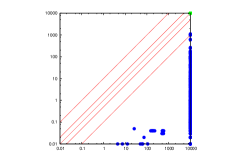
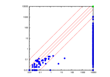
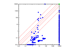
MathSAT-ceil

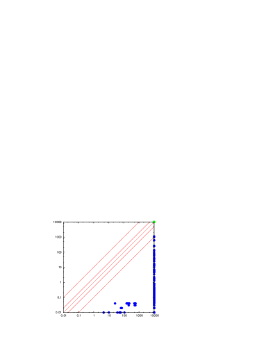
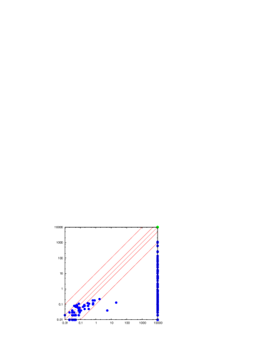
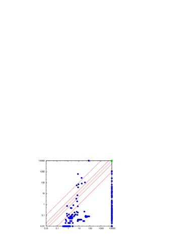
Figure 3. Comparison between MathSAT and the other $\mathcal{LA}(\mathbb{Z})$-interpolating tools, execution time.

5.1.1. Comparison with the state-of-the-art tools available

We compare MathSAT with all the other interpolant generators for $\mathcal{LA}(\mathbb{Z})$ which are available (to the best of our knowledge): iPrincess [BKRW10], InterpolatingOpenSMT [KLR10], and SmtInterpol . We compare not only the execution times for generating interpolants, but also the size of the generated formulas (measured in terms of number of nodes in their DAG representation).

For MathSAT, we use two configurations: MathSAT-modEq, which produces interpolants with modular equations using the Strengthen rule of §3, and MathSAT-ceil, which uses the ceiling function and the Division rule of §4.

Results on execution times for generating interpolants are reported in Fig. 3. Both MathSAT-modEq and MathSAT-ceil could successfully generate an interpolant for 478 of the 513 interpolation problems (timing out on the others), whereas iPrincess, InterpolatingOpenSMT and SmtInterpol were able to successfully produce an interpolant in 62, 192 and 217 cases respectively. Therefore, MathSAT can solve more than twice as many instances as its closer competitor SmtInterpol, and in most cases with a significantly shorter execution time (Fig. 3).

	iPrincess	InterpolatingOpenSMT	SmtInterpol
MathSAT-modEq
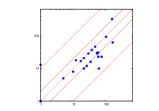
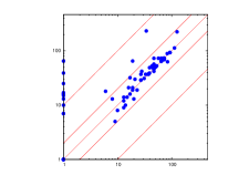
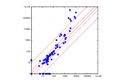
MathSAT-ceil

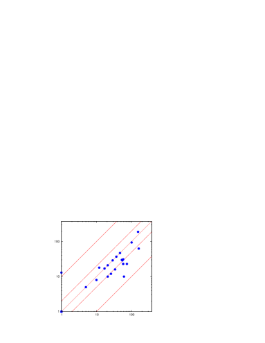
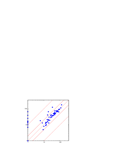
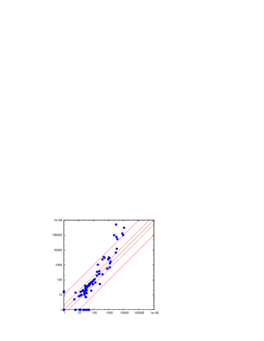
Figure 4. Comparison between MathSAT and the other $\mathcal{LA}(\mathbb{Z})$-interpolating tools, interpolants size (measured in number of nodes in the DAG of the interpolant). (See also footnote 12.)

For the subset of instances which could be solved by at least one other tool, therefore, the two configurations of MathSAT seem to perform equally well. The situation is the same also when we compare the sizes of the produced interpolants, measured in number of nodes in a DAG representation of formulas. Comparisons on interpolant size are reported in Fig. 4, which shows that, on average, the interpolants produced by MathSAT are comparable to those produced by other tools. In fact, there are some cases in which SmtInterpol produces significantly-smaller interpolants, but we remark that MathSAT can solve 261 more instances than SmtInterpol.

	Execution Time	Interpolants Size	Execution Time
MathSAT-ceil
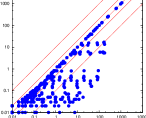
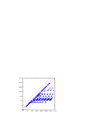
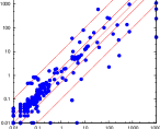
	MathSAT-modEq	MathSAT-modEq	MathSAT w/o interpolation
	(a)		(b)

Figure 5. (a) Comparison between MathSAT-modEq and MathSAT-ceil configurations for interpolation. (b) Execution time overhead for interpolation with MathSAT-ceil.

The differences between MathSAT-modEq and MathSAT-ceil become evident when we compare the two configurations directly. The plots in Fig. 5(a) show that MathSAT-ceil is dramatically superior to MathSAT-modEq, with gaps of up to two orders of magnitude in execution time, and up to four orders of magnitude in the size of interpolants. Such differences are solely due to the use of the ceiling function in the generated interpolants, which prevents the blow-up of the formula wrt. the size of the proof of unsatisfiability. Since most of the differences between the two configurations occur in benchmarks that none of the other tools could solve, the advantage of using ceilings was not visible in Figs. 3 and 4.

Finally, in Fig. 5(b) we compare the execution time of producing interpolants with MathSAT-ceil against the solving time of MathSAT with interpolation turned off. The plot shows that the restriction on the kind of extended branch-and-bound lemmas generated when computing interpolants (see §3.3) can have a significant impact on individual benchmarks. However, on average MathSAT-ceil is not worse than the “regular” MathSAT, and the two can solve the same number of instances, in approximately the same total execution time.

5.2. Experiments on model checking problems

Table 1. Experimental results on model checking problems.

	Results (num. of queries / execution time)
	MathSAT-ceil	MathSAT-modEq	MathSAT-noEQ	MathSAT-noBB
byte_add_1	9 / 1.05	9 / 1.06	9 / 1.00	9 / 1.02
byte_add_2	13 / 2.33	13 / 2.36	13 / 2.27	13 / 2.40
byte_add_3	52 / 97.68	52 / 91.71	T.O.	52 / 97.83
byte_add_4	28 / 27.77	28 / 28.38	T.O.	28 / 28.06
jain_1	8 / 0.04	8 / 0.04	T.O.	8 / 0.04
jain_2	8 / 0.06	8 / 0.06	T.O.	8 / 0.05
jain_4	7 / 0.06	7 / 0.06	T.O.	7 / 0.05
jain_5	42 / 0.84	42 / 0.82	42 / 0.88	42 / 0.81
jain_6	7 / 0.06	7 / 0.06	T.O.	7 / 0.06
jain_7	8 / 0.08	8 / 0.08	T.O.	8 / 0.07
num_conversion_1	51 / 13.33	51 / 13.02	51 / 21.04	51 / 12.83
num_conversion_2	T.O.	T.O.	T.O.	T.O.
num_conversion_3	43 / 5.40	43 / 5.02	43 / 5.78	43 / 4.99
num_conversion_4	52 / 19.03	53 / 19.81	T.O.	52 / 17.45
num_conversion_5	47 / 8.63	47 / 7.87	T.O.	47 / 7.72

	Results (num. of queries / execution time)
	MathSAT-noEQ-noBB	SmtInterpol	iPrincess	InterpolatingOpenSMT
byte_add_1	9 / 1.60	9 / 46.48	T.O.	1 / 0.073
byte_add_2	13 / 3.03	9 / 48.37	T.O.	1 / 0.073
byte_add_3	52 / 111.89	ERR	T.O.	BAD
byte_add_4	28 / 44.19	ERR	T.O.	BAD
jain_1	T.O.	7 / 2.15	8 / 23.44	BAD
jain_2	T.O.	BAD	6 / 20.12	BAD
jain_4	T.O.	7 / 2.93	9 / 55.05	BAD
jain_5	42 / 0.81	BAD	T.O.	BAD
jain_6	T.O.	BAD	7 / 28.96	BAD
jain_7	T.O.	BAD	T.O.	BAD
num_conversion_1	51 / 11.44	BAD	T.O.	BAD
num_conversion_2	T.O.	ERR	T.O.	BAD
num_conversion_3	43 / 5.36	ERR	T.O.	BAD
num_conversion_4	60 / 37.86	BAD	T.O.	BAD
num_conversion_5	47 / 8.10	ERR	T.O.	BAD
Key: T.O.: time-out (300 seconds); ERR: internal error/crash of the interpolating solver; BAD: wrong interpolant produced.

In the second part of our experimental analysis, we evaluate the performance of MathSAT and all the other interpolant generators for $\mathcal{LA}(\mathbb{Z})$ described above (§5.1.1) when used in an interpolation-based model checking context. In particular, we have implemented the original interpolation-based model checking algorithm of McMillan [McM03], and applied it to the verification of some transition systems generated from simple sequential C programs, using $\mathcal{LA}(\mathbb{Z})$ as a background theory. The benchmarks have been taken from the literature on $\mathcal{LA}(\mathbb{Z})$-related interpolation procedures [JCG08, Gri11]. We have then run this implementation using each of the solvers above as interpolation engines, and compared the results in terms of number of instances solved, time spent in computing interpolants, and number of calls to the interpolating solvers. For MathSAT, besides the two configurations MathSAT-modEq and MathSAT-ceil described in the previous section, we have also tested additional configurations obtained by disabling some of the layers of the $\mathcal{LA}(\mathbb{Z})$-solver described in §2.2: MathSAT-noEQ in which we disabled the equality elimination module, MathSAT-noBB in which we disabled the internal branch and bound module, and MathSAT-noEQ-noBB in which we disabled both.

The results are reported in Table 1. They clearly show that both MathSAT-ceil and MathSAT-modEq outperform the other tools also when applied in a model checking context. Moreover, it is interesting to observe the following: $\bullet$

for these particular benchmarks, MathSAT-modEq and MathSAT-ceil seem to be substantially equivalent: the only significant difference is in the num_conversion_4 benchmark, in which MathSAT-ceil leads to a slightly faster convergence, requiring one interation less;

the equality elimination layer seems to be very important, and disabling it leads to a dramatic decrease in performance;

somewhat surprisingly, the decrease in performance due to the disabling of the equality elimination module can be mitigated by disabiling also the internal branch and bound module. We attribute this to the different “quality” of the interpolants generated, which seems to be somehow “better” for MathSAT-noEq-noBB than for MathSAT-noEQ. However, we remark that the notion of “quality” of interpolants is still vague and unclear, and in particular we are not aware of any satisfactory characterization of it in the literature. Investigating the issue more in depth could be part of interesting future work.

6. Related Work

The general algorithm for interpolation in $\text{SMT}(\mathcal{T})$ was given by McMillan in [McM05], together with algorithms for sets of literals in the theories $\mathcal{EUF}$, $\mathcal{LA}(\mathbb{Q})$ and their combination. Algorithms for other theories and/or alternative approaches are presented in [RSS10, YM05, KW07, KMZ06, CGS10, JCG08, LT08, FGG⁺09, GKT09, BKRW10, KLR10]. In particular, [CGS10, FGG⁺09, GKT09] explicitly focus on building efficient interpolation procedures on top of state-of-the-art SMT solvers. Efficient interpolation algorithms for the Difference Logic and Unit-Two-Variables-Per-Inequality fragments of $\mathcal{LA}(\mathbb{Z})$ are given in [CGS10]. Some preliminary work on interpolation on the theory of fixed-width bit-vectors is presented in [KW07, Gri11]. As regards interpolation in the full $\mathcal{LA}(\mathbb{Z})$, McMillan showed in [McM05] that it is in general not possible to obtain quantifier-free interpolants (starting from a quantifier-free input) in the standard signature of $\mathcal{LA}(\mathbb{Z})$ (consisting of Boolean connectives, integer constants and the symbols $+,\cdot,\leq,=$). By extending the signature to contain modular equalities (or, equivalently, divisibility predicates) it is possible to compute quantifier-free $\mathcal{LA}(\mathbb{Z})$ interpolants by means of quantifier elimination, which is however prohibitively expensive in general, both in theory and in practice. Using modular equalities, Jain et al. [JCG08] developed polynomial-time interpolation algorithms for linear equations and disequations and for linear modular equations. A similar algorithm was also proposed in [LT08]. The work in [BKRW10] was the first to present an interpolation algorithm for the full $\mathcal{LA}(\mathbb{Z})$ (augmented with divisibility predicates) not based on quantifier elimination. Finally, an alternative algorithm, exploiting efficient interpolation procedures for $\mathcal{LA}(\mathbb{Q})$ and for linear equations in $\mathcal{LA}(\mathbb{Z})$, has been recently presented in [KLR10].

7. Conclusions

In this article, we have presented a novel interpolation algorithm for $\mathcal{LA}(\mathbb{Z})$ that allows for producing interpolants from arbitrary cutting-plane proofs without the need of performing quantifier elimination. We have also shown how to exploit this algorithm, in combination with other existing techniques, in order to implement an efficient interpolation procedure on top of a state-of-the-art $\text{SMT}(\mathcal{LA}(\mathbb{Z}))$-solver, with almost no overhead in search, and with up to orders of magnitude improvements – both in execution time and in formula size – wrt. existing techniques for computing interpolants from arbitrary cutting-plane proofs.

References

• [BKRW10] Angelo Brillout, Daniel Kroening, Philipp Rümmer, and Thomas Wahl. An Interpolating Sequent Calculus for Quantifier-Free Presburger Arithmetic. In Proc. IJCAR, volume 6173 of LNCS. Springer, 2010.
• [BNOT06] C. Barrett, R. Nieuwenhuis, A. Oliveras, and C. Tinelli. Splitting on Demand in SAT Modulo Theories. In Proc. LPAR’06, volume 4246 of LNCS. Springer, 2006.
• [BSST09] C. W. Barrett, R. Sebastiani, S. A. Seshia, and C. Tinelli. Satisfiability Modulo Theories. In Handbook of Satisfiability, chapter 25. IOS Press, 2009.
• [CGS10] A. Cimatti, A. Griggio, and R. Sebastiani. Efficient Generation of Craig Interpolants in Satisfiability Modulo Theories. ACM Trans. Comput. Logic, 12(1), October 2010.
• [DDA09] I. Dillig, T. Dillig, and A. Aiken. Cuts from Proofs: A Complete and Practical Technique for Solving Linear Inequalities over Integers. In Proc. CAV’09, volume 5643 of LNCS. Springer, 2009.
• [DdM06] B. Dutertre and L. de Moura. A Fast Linear-Arithmetic Solver for DPLL(T). In Proc. CAV’06, volume 4144 of LNCS. Springer, 2006.
• [FGG+09] A. Fuchs, A. Goel, J. Grundy, S. Krstic, and C. Tinelli. Ground interpolation for the theory of equality. In Proc. TACAS’09, volume 5505 of LNCS. Springer, 2009.
• [GKT09] A. Goel, S. Krstic, and C. Tinelli. Ground Interpolation for Combined Theories. In Proc. CADE-22, volume 5663 of LNCS. Springer, 2009.
• [GLS11] A. Griggio, T.T.H. Le, and R. Sebastiani. Efficient interpolant generation in satisfiability modulo linear integer arithmetic. In Parosh Abdulla and K. Leino, editors, Tools and Algorithms for the Construction and Analysis of Systems, volume 6605 of Lecture Notes in Computer Science, pages 143–157. Springer, 2011.
• [Gri11] Alberto Griggio. Effective word-level interpolation for software verification. In Per Bjesse and Anna Slobodova, editors, Proc. Formal Methods in Computer Aided Design - FMCAD11, 2011.
• [Gri12] Alberto Griggio. A Practical Approach to Satisability Modulo Linear Integer Arithmetic. Journal on Satisfiability, Boolean Modeling and Computation - JSAT, 8(1/2):1–27, 2012.
• [HJMM04] T. A. Henzinger, R. Jhala, R. Majumdar, and K. L. McMillan. Abstractions from proofs. In Proc. POPL’04. ACM, 2004.
• [JCG08] H. Jain, E. M. Clarke, and O. Grumberg. Efficient Craig Interpolation for Linear Diophantine (Dis)Equations and Linear Modular Equations. In Proc. CAV’08, volume 5123 of LNCS. Springer, 2008.
• [KLR10] Daniel Kroening, Jérome Leroux, and Philipp Rümmer. Interpolating Quantifier-Free Presburger Arithmetic. In Proc. LPAR, LNCS. Springer, 2010.
• [KMZ06] D. Kapur, R. Majumdar, and C. G. Zarba. Interpolation for data structures. In Proc. FSE’05. ACM, 2006.
• [KW07] D. Kroening and G. Weissenbacher. Lifting Propositional Interpolants to the Word-Level. In Proc. FMCAD’07, Los Alamitos, CA, USA, 2007. IEEE Computer Society.
• [LT08] C. Lynch and Y. Tang. Interpolants for Linear Arithmetic in SMT. In Proc. ATVA’08, volume 5311 of LNCS. Springer, 2008.
• [McM03] K. L. McMillan. Interpolation and SAT-Based Model Checking. In Proc. CAV’03, volume 2725 of LNCS. Springer, 2003.
• [McM05] K. L. McMillan. An interpolating theorem prover. Theor. Comput. Sci., 345(1), 2005.
• [McM06] K. L. McMillan. Lazy Abstraction with Interpolants. In Proc. CAV’06, volume 4144 of LNCS. Springer, 2006.
• [Pud97] P. Pudlák. Lower bounds for resolution and cutting planes proofs and monotone computations. J. of Symb. Logic, 62(3), 1997.
• [Pug91] W. Pugh. The Omega test: a fast and practical integer programming algorithm for dependence analysis. In Proc. SC, 1991.
• [RSS10] Andrey Rybalchenko and Viorica Sofronie-Stokkermans. Constraint solving for interpolation. J. Symb. Comput., 45(11), 2010.
• [Sch86] A. Schrijver. Theory of Linear and Integer Programming. Wiley, 1986.
• [Tse68] G. S. Tseitin. On the complexity of derivation in propositional calculus. Studies in Constructive Mathematics and Mathematical Logic, Part 2, 1968.
• [YM05] G. Yorsh and M. Musuvathi. A combination method for generating interpolants. In Proc. CADE-20, volume 3632 of LNCS. Springer, 2005.