Towards a Shape Analysis for
Graph Transformation Systems

Abstract

Graphs and graph transformation systems are a frequently used modelling technique for a wide range of different domains, covering areas as diverse as refactorings, network topologies or reconfigurable software. Being a formal method, graph transformation systems lend themselves to a formal analysis. This has inspired the development of various verification methods, in particular also model checking tools.

In this paper, we present a verification technique for infinite-state graph transformation systems. The technique employs the abstraction principle used in shape analysis of programs, summarising possibly infinitely many nodes thus giving shape graphs. The technique has been implemented using the $3$-valued logical foundations of standard shape analysis. We exemplify the approach on an example from the railway domain.

1 Introduction

Graph transformation systems (GTSs, [CMR⁺97]) have - in particular due to their visual appeal - become a widely used technique for system modelling. They are employed in numerous different areas, ranging from the specification of visual contracts for software to dynamically evolving systems. They serve as a formally precise description of the behaviour of complex systems. Often, such systems are operating in safety critical domains (e.g. railway, automotive) and their dependability is of vital interest. Hence, a number of approaches for the analysis of graph transformation systems have been developed [Tae03], in particular also model checking techniques [RSV04, SV03, Ren03, BCK08, BBKR08, SWJ08]. Model checking allows to fully automatically show properties of system models, for instance for properties specified in temporal logic. Model checking proceeds by exploring the whole state space of a model, i.e. in case of graph transformation systems by generating the set of graphs which are reachable from a given start graph by means of rule application. While existing tools have proven to be able to tackle also large state spaces, standard model checking techniques fail when the state space becomes infinite.

There are, in general, two approaches to dealing with very large or even infinite state spaces. The first approach is to devise a clever way of selecting a finite subset of states which is sufficient for proving the desired properties, effectively constructing an under-approximation of the system. This concept is explored e.g. in bounded model checking [BCC⁺03]. The second approach is to construct an abstraction, i.e. a finite representation of a superset of the state space. This over-approximation of the system is then used to show certain properties of the original system.

In this paper, we propose an new approach towards a verification technique for infinite state graph transformation systems using over-approximation. The technique follows the idea of shape analysis algorithms for programs [SRW02] which are used to compute properties of a program’s heap structures. Shape analyses compute abstractions of heap states by collapsing certain sets of identical nodes into so-called summary nodes. Thereby, an infinite number of heap states can be finitely represented. Such shapes can be used to derive structural properties about the heap.

This principle of summarisation in GTSs has already been presented in numerous other works, for example Rensink et al.  [Ren04, RD06] or Bauer et.al. [BBKR08] which introduce so-called abstract graph transformations. Our approach is set apart from these by strict adherence to the formalism presented in [SRW02], which immensely simplifies implementation and gives us a level of parametrization that other approaches lack. A more thorough discussion of advantages of our approach over related work will be presented in section 6.

Here, we present a shape analysis for GTSs which is directly based on the $3$-valued logical foundations of standard shape analysis. Given this logical basis for shape graphs, we define rule application on shape graphs via a constructive definition of materialisation and summarisation. The technique can thus be directly implemented as defined, even re-using parts of the logical machinery of TVLA [BLARS07], the most prominent shape analysis tool. In order to illustrate our technique, we exemplify it on a simple GTS model from the railway domain.

The paper is structured as follows. The next section will give the basic definitions for our approach. Section 3 introduces materialisation and summarisation on graphs and thereby defines the application of rules on shape graphs. Section 4 shows the correctness of our approach, i.e. shows that by rule application on shape graphs an overapproximation of the set of reachable graphs is computed. The next section then reports on the implementation. Finally, Sect. 6 concludes, further discusses related work and gives some directions for future research.

2 Background

This section introduces the basic definitions that are required to formulate our main results. To illustrate the definitions in this section, we use the following example from the rail domain. A rail network is given by a set of stations (S) and a set of rail sections, called tracks (T), connected by a relation called “next”. Vehicles, called “railcabs” (RC), possibly with passengers (P) travel on the tracks. The example is a simplified version of a case study coming from the project “Neue Bahntechnik Paderborn”.

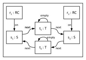
Figure 1: A simple rail network

Figure 1 shows a graph depicting one configuration of such a rail network. Configurations can change in a number of ways, for instance by passengers entering railcabs and railcabs moving on tracks according to predefined protocols. The overall goal is to show certain safety properties (e.g. collision avoidance) for arbitrary networks. We first of all start by defining some basic notions on graphs.

Definition 1

A graph $G$ is a pair $(N,E)$, where $N$ is a set of nodes and $E\subseteq N\times{\cal L}\times N$ is a set of labelled edges for some label set $\cal L$. For any graph $G$, $N_{G}$ and $E_{G}$ denote its node and edge sets, respectively.

This definition restricts the class of graphs we are considering to those in which no more than a single same-labelled edge may exist between any two nodes. The generic concept of a morphism extends to these graphs in a natural way.

Definition 2

For graphs $G$ and $H$, a morphism $f:G\rightarrow H$ is a function $f:N_{G}\rightarrow N_{H}$ extended to edges by $f\left(n,l,n^{\prime}\right)=\left(f(n),l,f\left(n^{\prime}\right)\right)$ such that $f\left(E_{G}\right)\subseteq E_{H}$.

Figure 1 shows a graph representing one very simple rail network consisting of two stations which are connected by two tracks. Note that we include a simple notion of typing in the graph. The type of a node is represented by a loop labelled with the name of the type. Such type loops are not displayed as edges but rather as part of the node name. Thus, instead of displaying a self-edge of $r_{1}$ labelled “RC”, we label the node $r_{1}:RC$.

In order to model the dynamic behaviour of a system represented by a graph, we need to transform graphs into other graphs. For this, graph production rules can be used. In this paper, we take an operational, not categorical, view on graph transformation. As a consequence, we favour a simple approach to graph production rules, as the following definitions show.

Definition 3

A graph production rule $P=\left\langle L,R\right\rangle$ consists of two graphs $L$ and $R$ called the left hand side and the right hand side, respectively.

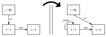
Figure 2: Rule $EnterStation$

Figure 2 shows an example of a rule which describes a railcab entering a station. In addition, we have rules for leaving a station, for movement of single as well as convoys of railcabs and for forming convoys (all elided due to space restrictions). In the rules, we use node names instead of injective morphisms to identify nodes appearing in the left as well as right hand side. Aside from this technicality we use the standard SPO approach to rule definition and application [Löw93]. In order to make node creation and deletion explicit, we use the following sets:

$$N^{-}=N_{L}\setminus N_{R},\ E^{-}=E_{L}\setminus E_{R}$$ (deleted nodes and edges)

$$N^{+}=N_{R}\setminus N_{L},\ E^{+}=E_{R}\setminus E_{L}$$ (created nodes and edges)

These sets are used to define the effect of an application of a production rule on a graph $G$.

Definition 4

Let $P$ be a production rule, $G$ a graph. The rule $P=\left\langle L,R\right\rangle$ can be applied on G if we can find an injective morphism $m:L\rightarrow G$ (called a matching).
If $m$ is a matching, then the application of $P$ onto $G$ with matching $m$ is the graph

$$H =\left(N_{H},E_{H}\right)\ \mbox{with}$$

$$N_{H} =\left(N_{G}\setminus m\left(N^{-}\right)\right)\stackrel{{\scriptstyle.}}{{\cup}}N^{+}$$

$$E_{H} =\left(\left(E_{G}\setminus m\left(E^{-}\right)\right)\cup\widehat{m}\left(E^{+}\right)\right)\cap\left(N_{H}\times\mathcal{L}\times N_{H}\right)$$

where $\widehat{m}=m\cup\operatorname{id}_{N^{+}}$.

For this production application we write $G\mathrel{\lower 1.0pt\hbox{$\mathrel{-}_{\vphantom{{}}}\mkern-8.0mu\stackrel{{\scriptstyle P,m}}{{\cleaders\hbox{$\smash{\mkern-2.0mu\mathord{-}\mkern-2.0mu}$}\hfill\vphantom{\lower 1.0pt\hbox{$\rightarrow$}}_{\vphantom{{}}}}}\mkern-11.0mu\rightarrow$}}H$. Similarly, $G\mathrel{\lower 1.0pt\hbox{$\mathrel{-}_{\vphantom{{}}}\mkern-8.0mu\stackrel{{\scriptstyle P}}{{\cleaders\hbox{$\smash{\mkern-2.0mu\mathord{-}\mkern-2.0mu}$}\hfill\vphantom{\lower 1.0pt\hbox{$\rightarrow$}}_{\vphantom{{}}}}}\mkern-11.0mu\rightarrow$}}H$ holds if there is some $m$ such that $G\mathrel{\lower 1.0pt\hbox{$\mathrel{-}_{\vphantom{{}}}\mkern-8.0mu\stackrel{{\scriptstyle P,m}}{{\cleaders\hbox{$\smash{\mkern-2.0mu\mathord{-}\mkern-2.0mu}$}\hfill\vphantom{\lower 1.0pt\hbox{$\rightarrow$}}_{\vphantom{{}}}}}\mkern-11.0mu\rightarrow$}}H$ and $G\longrightarrow H$ if there is furthermore a production rule $P$ such that $G\mathrel{\lower 1.0pt\hbox{$\mathrel{-}_{\vphantom{{}}}\mkern-8.0mu\stackrel{{\scriptstyle P}}{{\cleaders\hbox{$\smash{\mkern-2.0mu\mathord{-}\mkern-2.0mu}$}\hfill\vphantom{\lower 1.0pt\hbox{$\rightarrow$}}_{\vphantom{{}}}}}\mkern-11.0mu\rightarrow$}}H$. We let $\mathord{\mathrel{\lower 1.0pt\hbox{$\mathrel{-}_{\vphantom{{}}}\mkern-8.0mu\stackrel{{\scriptstyle~{}}}{{\cleaders\hbox{$\smash{\mkern-2.0mu\mathord{-}\mkern-2.0mu}$}\hfill\vphantom{\lower 1.0pt\hbox{$\rightarrow$}}_{\vphantom{{}}}}}\mkern-11.0mu\rightarrow$}}}^{*}$ denote the transitive and reflexive closure of $\mathord{\mathrel{\lower 1.0pt\hbox{$\mathrel{-}_{\vphantom{{}}}\mkern-8.0mu\stackrel{{\scriptstyle~{}}}{{\cleaders\hbox{$\smash{\mkern-2.0mu\mathord{-}\mkern-2.0mu}$}\hfill\vphantom{\lower 1.0pt\hbox{$\rightarrow$}}_{\vphantom{{}}}}}\mkern-11.0mu\rightarrow$}}}$. With these definitions at hand, we can define the set of reachable graphs of a graph transformation system (or graph grammar, as it includes a start graph).

Definition 5

A graph transformation system $GT=(G_{0},\left(P_{i}\right)_{i\in I})$ consists of a start graph $G_{0}$ and a set of production rules $P_{i},i\in I$. The set of reachable graphs of a graph transformation system $GT$ is

$$\halign to=433.62pt{\zstrut\z@left\z@startline\ignorespaces$\@lign#$\z@stopline\hfil&\hbox to 0pt{\hss\@lign#}\cr\hbox{\hskip 0.0pt\hbox{\hbox{}\hbox{\ignorespaces\ignorespaces$reach(GT)=\{G\mid G_{0}\mathrel{\lower 1.0pt\hbox{$\mathrel{-}_{\vphantom{{}}}\mkern-8.0mu\stackrel{{\scriptstyle}}{{\cleaders\hbox{$\smash{\mkern-2.0mu\mathord{-}\mkern-2.0mu}$}\hfill\vphantom{\lower 1.0pt\hbox{$\rightarrow$}}_{\vphantom{{}}}}}\mkern-11.0mu\rightarrow$}}^{*}G\}$}}}\crcr}$$

In this paper we are interested in proving properties of the set of all reachable graphs. A property can for instance be the absence of forbidden patterns, i.e. substructures, in a graph (or the presence of desired patterns).

Such a forbidden pattern can be defined by a production rule of the form $$P=\left\langle F,F\right\rangle G G\models F$$ (with left and right hand equal). The pattern is present in a graph () if the rule matches. A forbidden pattern for our example is given on the right hand side. It specifies a collision of two railcabs (two railcabs on one track).

The set of reachable graphs can in general be infinite (e.g. for our example, if we introduce a rule which allows new passengers to be created). The objective of this paper is to construct an abstraction (and overapproximation) of this set of reachable graphs which is finite but on which we can still show properties.

Before doing so, we need to look a bit closer into the basic technology behind shape analysis. Shape analysis algorithms operate on logical a structure using first order logic to formulate properties. In the following, we closely follow [SRW02] in our notations. Note, however, that we explicitly exclude the notion of transitive closure from [SRW02], since transitivity would violate the important locality property of rule applications. The word formula always refers to a first order formula over a set of predicate symbols $\mathcal{P}$ and variables $\mathcal{V}$. Variables are assigned values from some domain (or universe) $U$, and $k$-ary predicates $\mathcal{P}_{k}$ are interpreted by truth-valued functions, i.e. we have an interpretation function $\iota:{\mathcal{P}_{k}}\rightarrow(U^{k}\rightarrow{\mathcal{T}})$ ( $\mathcal{T}$ a set of truth values). We let $\mathcal{F}\left(\varphi\right)$ denote the set of free variables of a formula $\varphi$. Domain, predicates and interpretation function together make up a logical structure $S=\left\langle U,\mathcal{P},\iota\right\rangle$, sometimes also abbreviated by $\left\langle U,\iota\right\rangle$. For a formula $\varphi$, $\llbracket\varphi\rrbracket_{m}^{S}$ denotes the value of $\varphi$ in the structure $S$ under an assignment $m$.

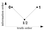
Figure 3: Kleene logic with logical and information order

A logical structure is called $n$-valued if for the target set $\mathcal{T}$ of the predicates $\left\lvert\mathcal{T}\right\rvert=n$ holds. Two sets of truth values will play a role here: the ordinary boolean values ($\mathcal{T}=\{\mathbf{0},\mathbf{1}\}$) and the three-valued set of Kleene logic ($\mathcal{T}=\{\mathbf{0},\mathbf{1},\mbox{{\textonehalf}}\}$, values called $false$, $true$ and $maybe$). On the truth values of Kleene logic we have two different orderings (see Fig. 3), one reflecting the amount of information ($\sqsubseteq$) present in a logical value, the other the logical truth ($\leq$). That is, for $l_{1},l_{2}\in\mathcal{T}=\left\{\mathbf{0},\mbox{{\textonehalf}},\mathbf{1}\right\}$:

$$l_{1}\sqsubseteq l_{2} \Leftrightarrow\left(l_{1}=l_{2}\right)\vee\left(l_{2}=\mbox{{\textonehalf}}\right)$$

$$l_{1}\leq l_{2} \Leftrightarrow\left(l_{1}=l_{2}\right)\vee\left(l_{1}=\mathbf{0}\right)\vee\left(l_{1}=\mbox{{\textonehalf}}\wedge l_{2}=\mathbf{1}\right)$$

Our final goal is to represent graphs as well as their abstractions by logical structures, the former by 2-valued and the latter by 3-valued. To this end, we partition the set $\mathcal{P}$ into the sets of so-called core predicates $\mathcal{C}$ and instrumentation predicates $\mathcal{I}$. Later on, $\mathcal{C}$ will encode basic properties (like $next$-relations between nodes), while $\mathcal{I}$ will be used to increase the precision of the analysis with respect to a given property. The set $\mathcal{C}$ is further subdivided into unary core predicates $\mathcal{C}^{1}$ (used e.g. for types) and binary core predicates $\mathcal{C}^{2}$. One specific predicate called summarised ($sm$) is used in the abstraction: a summarised node can represent lots of concrete nodes. In ordinary graphs no nodes are summarised.

The encoding of graphs as logical structures then works as follows: The set of nodes $N$ of a graph will be represented by the domain set $U$. The edge labels $\mathcal{L}$ will give us the set of predicate symbols $\mathcal{P}$, and particular edges are encoded by $\iota$. Table 1 gives the logical structure of the rail network of Fig. 1.

$$U =\left\{r_{1},r_{2},s_{1},s_{2},t_{1},t_{2}\right\}$$

$$\mathcal{C}^{1} =\left\{RC,T,S,sm\right\},\mathcal{C}^{2}=\left\{on,next\right\}$$

$\iota\left(\mathcal{C}^{1}\right)$	$RC$	$T$	$S$	$sm$	$\iota\left(on\right)$	$r_{1}$	$r_{2}$	$s_{1}$	$s_{2}$	$t_{1}$	$t_{2}$	$\iota\left(next\right)$	$r_{1}$	$r_{2}$	$s_{1}$	$s_{2}$	$t_{1}$	$t_{2}$
$r_{1}$	$1$	$0$	$0$	$0$		$0$	$0$	$1$	$0$	$0$	$0$		$0$	$0$	$0$	$0$	$0$	$0$
$r_{2}$	$1$	$0$	$0$	$0$		$0$	$0$	$0$	$1$	$0$	$0$		$0$	$0$	$0$	$0$	$0$	$0$
$s_{1}$	$0$	$0$	$1$	$0$		$0$	$0$	$0$	$0$	$0$	$0$		$0$	$0$	$0$	$0$	$1$	$0$
$s_{2}$	$0$	$0$	$1$	$0$		$0$	$0$	$0$	$0$	$0$	$0$		$0$	$0$	$0$	$0$	$0$	$1$
$t_{1}$	$0$	$1$	$0$	$0$		$0$	$0$	$0$	$0$	$0$	$0$		$0$	$0$	$0$	$1$	$0$	$0$
$t_{2}$	$0$	$1$	$0$	$0$		$0$	$0$	$0$	$0$	$0$	$0$		$0$	$0$	$1$	$0$	$0$	$0$

Table 1: Logical structure of the graph in Figure 1

Definition 6

Let $G$ be a graph. The $2$-valued encoding of $G$, denoted $ls\left(G\right)$, is a $2$-valued logical structure $S=\left\langle U,\mathcal{P},\iota\right\rangle$ with $U=N_{G}$, $\mathcal{C}^{1}\cup\mathcal{C}^{2}=\mathcal{P}=\mathcal{L}$ and $\iota$ defined by:

• For $p\in\mathcal{C}^{2}$: $\iota\left(p\right)\left(u_{1},u_{2}\right)=1\Leftrightarrow\left(u_{1},p,u_{2}\right)\in E_{G}$,

• For $p\in\mathcal{C}^{1}$: $\iota\left(p\right)\left(u\right)=1\Leftrightarrow\left(u,p,u\right)\in E_{G}$,

• For $sm$: $\iota\left(sm\right)\left(u\right)=0$.

The basic idea of shape analysis is to represent infinitely many different but in shape similar configurations or graphs by one shape graph. A shape graph thus cannot always give us precise information about the number of nodes, nor can it give us precise information about edges between nodes. The third truth value “maybe” (½) is used to represent this fact in logical structures. A node representing many concrete nodes is summarised, denoted by a dashed rectangle, an edge which is only “maybe” there (dashed line) is assigned the truth value ½. Figure 4 shows a shape graph. Here, we for instance have $RC(r_{1})=\mathbf{1}$ ($r_{1}$ is definitely of type railcab), $sm(t)=\mbox{{\textonehalf}}$ (there is possibly more than one track) and $next(t,t)=\mbox{{\textonehalf}}$ (the tracks summarised in $t$ maybe connected). The predicate $is\leavevmode\vbox{\hrule width=3.99994pt}colliding$ will be explained later. This is the start shape graph of our reachability analysis.

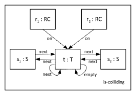
Figure 4: Start shape graph

Shape graphs are abstractions of concrete graphs, concrete graphs can be embedded into them. Clearly , the predicate $sm$ plays a crucial role in embeddings. Interpretations of this predicate are restricted to values $\mathbf{0}$ and ½. If it is ½ for an individual $u$, this means $u$ may or may not stand for a whole set of nodes. If it is $\mathbf{0}$ for $u$, then $u$ is guaranteed to represent a single individual.

We thus obtain the notion of embedding by the following definition.

Definition 7

Let $S=\left\langle U,\mathcal{P},\iota\right\rangle,S^{\prime}=\left\langle U^{\prime},\mathcal{P},\iota^{\prime}\right\rangle$ be two logical structures and $f:U\rightarrow U^{\prime}$ be a surjective function. We say that $f$ embeds $S$ in $S^{\prime}$ ($S\sqsubseteq S^{\prime}$) iff $\mathop{\mathstrut{\forall}}\nolimits k\mathop{\mathstrut{\forall}}\nolimits p\in\mathcal{P}_{k},\mathop{\mathstrut{\forall}}\nolimits u_{1},\ldots,u_{k}\in U$

$$\iota\left(p\right)\left(u_{1},\ldots,u_{k}\right)\sqsubseteq\iota^{\prime}\left(p\right)\left(f\left(u_{1}\right),\ldots,f\left(u_{k}\right)\right)$$ (1)

and $\mathop{\mathstrut{\forall}}\nolimits u^{\prime}\in U^{\prime}$

$$\left(\left\lvert\left\{u\mid f\left(u\right)=u^{\prime}\right\}\right\rvert>1\right)\sqsubseteq\iota^{\prime}\left(sm\right)\left(u^{\prime}\right)$$ (2)

Thus, intuitively, $S\sqsubseteq S^{\prime}$ means that $S^{\prime}$ is in some way a “generalisation” of $S$.

3 Rule Application on Shape Graphs

The basic idea of shape analysis follows that of abstract interpretation: instead of looking at concrete graphs and applying graph transformation rules concretely, we look at shape graphs and apply our rules to shapes instead. We thus inductively compute the set of reachable shape graphs and on these check for forbidden patterns. If the forbidden pattern is absent in this set, it should also not be present in any concretely reachable graph. In this section we will explain how to apply rules on shape graphs, the next section will look at the soundness of this technique.

Rule application on shape graphs involves a number of distinct steps, some of which are not present on concrete graphs. The basic difference is that due to the “maybe” predicates in shapes, we usually do not find an exact counterpart, i.e. an injective matching, for the left hand side. The following steps are necessary:

Match

To find out whether a rule $P$ matches, we evaluate a rule formula $\varphi_{P}$ in the logical structure of the shape graph. If it evaluates to ½, the rule can potentially be applied.

Focus

In order to actually apply a potentially applicable rule, we have to bring the left hand side of the rule into focus. We do so by materialising the left hand side in the shape graph.

Coerce

Materialisation concretises parts of the shape graph. This concretisation has an influence on the rest of the shape (e.g., if a railcab is definitely on one track, it cannot at the same time be “maybe” on another track). Coercing removes “maybe” structures in the shape by inspecting definitely known predicates.

Apply

After materialisation and coercion the rule can be applied, basically as on concrete graphs.

We next go through each of these steps. To define matching, we transform the left hand side of a rule into a formula.

Definition 8

Let $P=\left\langle L,R\right\rangle$ be a graph production rule. The production formula $\varphi_{P}$ corresponding to $P$ is given by

$$\varphi_{P}= \underbrace{\bigwedge_{\begin{subarray}{c}(n,l,n^{\prime})\in E_{L}\\ l\text{ binary}\end{subarray}}l\left(n,n^{\prime}\right)}_{\text{edges}}\wedge\underbrace{\bigwedge_{\begin{subarray}{c}\left(n,l,n\right)\in E_{L}\\ l\text{ unary}\end{subarray}}l\left(n\right)}_{\text{loops}}\wedge\underbrace{\bigwedge_{\begin{subarray}{c}n_{1},n_{2}\in N_{L}\\ n_{1}\neq n_{2}\end{subarray}}\neg\left(n_{1}=n_{2}\right)}_{\text{injectivity}}\wedge\underbrace{\bigwedge_{n\in N_{L}}\neg sm\left(n\right)}_{\text{non-summarisation}}$$

The $\neq$ here means the non-equality of the variable symbols, while $=$ is a regular predicate.

When this formula evaluates to ½ ($\mathbf{1}$) for a 3-valued structure, we say that the rule is potentially applicable (applicable) in the associated shape graph. To actually apply it, we have to bring the rule into focus, i.e. make sure that we definitely find the left hand side of the rule in the shape. Intuitively, we would want something like this

$$focus_{P}\left(S\right)=\left\{S^{\prime}\mid S^{\prime}\sqsubseteq S\wedge\mathop{\mathstrut{\exists}}\nolimits m:\llbracket\varphi_{P}\rrbracket_{m}^{S^{\prime}}=\mathbf{1}\right\}$$

meaning all possible graphs which are embeddable in $S$ and to which the rule can be applied. Unfortunately, this set can be infinitely large, and in fact, this is exactly what our technique tries to avoid, namely having to construct all concrete graphs for a shape. Instead, we only compute a set $mat_{P}\left(S\right)$ (the materialisation with respect to a rule) such that each element in $focus_{P}\left(S\right)$ can be embedded in at least one element from $mat_{P}\left(S\right)$, but still the rule is applicable in every shape in $mat_{P}\left(S\right)$.

In order to construct the set $mat_{P}\left(S\right)$, let us now assume that we have a shape graph $G$, its corresponding logical structure $S=\left\langle N_{G},\mathcal{L},\iota\right\rangle$, a production rule $P=\left\langle L,R\right\rangle$, and a matching $m:L\rightarrow N_{G}$ which gives rise to an assignment $\bar{m}:\mathcal{F}\left(\varphi_{P}\right)\rightarrow N_{G}$ such that $\llbracket\varphi_{P}\rrbracket_{\bar{m}}^{S}\neq\mathbf{0}$. Let $N_{G}^{sum}$ be the set of summary nodes in $G$. We have to exactly find the left hand side of the rule in the materialisation. Thus, every node $u$ in $\Gamma(m):=m(L)\cap N_{G}^{sum}$ needs to be materialised into as many nodes as are mapped onto $u$ via $m$. The relationship of these materialised node to other nodes of the shape are inherited from the original shape graph. In addition, we have to decide whether to keep the summarised node out of which have made our materialisation, or to remove it. This represents the idea that summarised nodes can stand for any number of concrete nodes. Thus we get several materialisations of one shape graph, one for every set $I\subseteq\Gamma(m)$, $I$ being those now materialised nodes for which we keep the original summary node.

Definition 9

Let $G$ be a graph, $S=ls\left(G\right)=\left\langle U,\mathcal{P},\iota\right\rangle$, $P=\left\langle L,R\right\rangle$ be a production rule and $\mathcal{M}=\left\{m\mid\llbracket\varphi_{P}\rrbracket_{\bar{m}}^{S}=\mbox{{\textonehalf}}\right\}$. Let $\Gamma\left(m\right):=m(L)\cap N_{G}^{sum}$. Then, for each $m\in\mathcal{M}$ and each $I\subseteq\Gamma\left(m\right)$ the materialisation of $P$ according to $\left(m,I\right)$ is defined as $mat_{m}^{I}\left(S\right)=\left\langle U^{I},\mathcal{P},\iota^{\prime}\right\rangle$, with

$$U^{I}=U\setminus\left(m\left(N_{L}\right)\setminus I\right)\cup N_{L}$$

and for $p\in\mathcal{C}^{2}$ and $q\in\mathcal{C}^{1}\setminus\left\{sm\right\}$, letting $\widehat{m}=m\cup id_{U}$:

$$\iota^{\prime}(q)(u) =\begin{cases}\mathbf{1}&\text{if }u\in N_{L}\wedge\left(u,q,u\right)\in E_{L}\\ \iota(q)\left(\widehat{m}\left(u\right)\right)&\text{else }\end{cases}$$

$$\iota^{\prime}(p)\left(u_{1},u_{2}\right) =\begin{cases}\mathbf{1}&\text{ if }u_{1},u_{2}\in N_{L}\wedge\left(u_{1},p,u_{2}\right)\in E_{L}\\ \iota(p)\left(\widehat{m}\left(u_{1}\right),\widehat{m}\left(u_{2}\right)\right)&\text{ else }\end{cases}$$

$$\iota^{\prime}(sm)(u) =\begin{cases}\mathbf{0}&\text{ if }u\in N_{L}\\ \iota(sm)\left(\widehat{m}\left(u\right)\right)&\text{ else }\end{cases}$$

The collection of all such logical structures is then defined as the materialisation of $S$ with respect to $P$:

$$mat_{P}\left(S\right) =\left\{S\mid\mathop{\mathstrut{\exists}}\nolimits m:\llbracket\varphi_{P}\rrbracket_{m}^{S}=\mathbf{1}\right\}$$ regular rule application

$$\cup\left\{mat_{m}^{I}\left(S\right)\mid\llbracket\varphi_{P}\rrbracket_{m}^{S}=\mbox{{\textonehalf}},I\subseteq\Gamma\left(m\right)\right\}$$ materialisations

Note that the size of $mat_{m}^{I}$ can be exponential in the number of nodes in the left hand side of the rule, but is finite. The following theorem states that it is indeed sufficient to consider $mat_{P}\left(S\right)$ instead of $focus_{P}\left(S\right)$.

Theorem 3.1

Let $S$ be a $3$-valued logical structure and $P$ a production rule. Then

$$mat_{P}\left(S\right) \subseteq focus_{P}\left(S\right)\text{ and}$$ (3)

$$focus_{P}\left(S\right) \sqsubseteq mat_{P}\left(S\right)$$ (4)

Due to lack of space we have to omit all proofs. They can be found in [SWW10]. Fig. 5 shows the result of applying materialisation on the starting shape graph using the $EnterStation$ production rule.

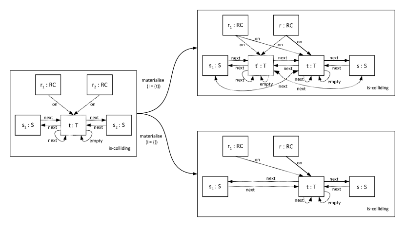
Figure 5: Materialisation of a shape graph wrt. $EnterStation$

The next step is coercion. After materialisation we apply the coerce operation defined in [SRW02] on the resulting shape graphs. Doing so serves two purposes: On the one hand we can identify inconsistencies in the shape graph (e.g. an empty track with a railcab on it). On the other hand we can “sharpen” some predicate values of the shape graph in some cases. The latter can be found, for example, when looking at the materialised shape graphs of Fig. 5. There, the $empty$ predicate has the value ½ for node $t$. Yet, the railcab $r$ is definitely on it. Hence, we can sharpen the predicate value of $empty$ to $\mathbf{0}$.

The semantic knowledge needed to perform the coercion step comes from the so-called compatibility constraints. Compatibility constraints may be either hand-written formulae (e.g. $\mathop{\mathstrut{\exists}}\nolimits r:on(r,t)\Rightarrow\neg empty(t)$) or may be formulae that are derived from the so-called meaning formulae of the instrumentation predicates (see below for an discussion of instrumentation predicates and its meaning formulae). We do not explain coercion in detail here, for this see [SWW10].

Finally, we can now apply the production rule. Since the left hand side of the rule is - due to materialisation - explicitly present in the shape graph, this follows the standard procedure. There is however one speciality, related to the analysis, involved. To make the analysis more precise, we introduce special instrumentation predicates to our shape graphs. Consider again our forbidden collision pattern of the last section. To see whether this is present, we could evaluate the formula

$$\varphi_{forbidden\leavevmode\vbox{\hrule width=2.79996pt}collision} :=on(r_{1},t)\wedge on(r_{2},t)\wedge T(t)\wedge RC(r_{1})\wedge RC(r_{2})\wedge$$

$$\phantom{=a}\neg(r_{1}=r_{2})\wedge\neg sm(r_{1})\wedge\neg sm(r_{2})\wedge\neg sm(t)$$

Unfortunately, for most shape graphs we find an assignment $m$ such that this formula evaluates to ½ under $m$ since we have lost information about the precise position of railcabs on tracks. This holds in particular also in our start shape graph. To regain this, we introduce an extra instrumentation predicate for this property: $is\leavevmode\vbox{\hrule width=3.99994pt}colliding$. In our start shape graph for the reachability analysis this predicate is $\mathbf{0}$ for all nodes (see Fig. 4 where the label $is\leavevmode\vbox{\hrule width=3.99994pt}colliding$ is not connected to any node; we thus start the analysis with a shape in which no two railcabs are on the same track). Every concretisation of a shape graph with instrumentation predicates $p$ has to obey its so-called meaning formula $\alpha_{P}$. For example the instrumentation predicate $is\leavevmode\vbox{\hrule width=3.99994pt}colliding$ has the following attached meaning formula:

$$\halign to=433.62pt{\zstrut\z@left\z@startline\ignorespaces$\@lign#$\z@stopline\hfil&\hbox to 0pt{\hss\@lign#}\cr\hbox{\hskip 0.0pt\hbox{\hbox{}\hbox{\ignorespaces\ignorespaces$\alpha_{is\leavevmode\vbox{\hrule width=2.79996pt}colliding}(v):=T(v)\wedge\mathop{\mathstrut{\exists}}\nolimits r_{1},r_{2}:(r_{1}\neq r_{2}\wedge on(r_{1},v)\wedge on(r_{2},v))$}}}\crcr}$$

Now, for a concrete graph $G$ embedded in a shape $S$ with node $v$ mapped to $u$ via the embedding function, we have to check that the evaluation of the meaning formula wrt. $v$ yields the same or a more precise value (wrt. to the information order) than the instrumentation predicate value in $u$. Instrumentation predicates are (obviously) not part of our production rules. Therefore, we have to explicitly specify how these predicates change on rule application. For this purpose, we specify update formulae.

Definition 10

A shape production rule $P=(\langle L,R\rangle,\gamma)$ consists of a graph production rule $\langle L,R\rangle$ and function $\gamma$ mapping from each instrumentation predicate $p\in\mathcal{I}$ and each node $v\in N_{R}$ to a first-order predicate-update formula $\varphi_{p,v}$ with free variables in $N_{L}$.

The predicate-update formula $\varphi_{p,v}$ specifies how the value of the instrumentation predicate $p$ should be calculated for each $v\in N_{R}$ of the new shape graph with respect to the predicate values of the old shape graph. For example, we could attach the following update formulae to the production rule $EnterStation$:

$$\varphi_{is\leavevmode\vbox{\hrule width=2.79996pt}colliding,r} =\mathbf{0},\quad\varphi_{is\leavevmode\vbox{\hrule width=2.79996pt}colliding,s}=\mathbf{0}$$

$$\varphi_{is\leavevmode\vbox{\hrule width=2.79996pt}colliding,t} =is\leavevmode\vbox{\hrule width=3.99994pt}colliding(t)\wedge{}$$

$$\phantom{=.}\mathop{\mathstrut{\exists}}\nolimits r_{2},r_{3}:((r_{2}\neq r)\wedge(r_{3}\neq r)\wedge(r_{3}\neq r_{2})\wedge on(r_{2},t)\wedge on(r_{3},t))$$

Note that we make use of a free variable called $r$ in the formula $\varphi_{is\leavevmode\vbox{\hrule width=2.79996pt}colliding,t}$. When the production rule is applied to a shape graph $S$, this free variable gets assigned to the individual in $S$ that represents the $r$ node of the left hand side of the production rule. The following definition formalises the shape production application.

Definition 11

Let $P=(\langle L,R\rangle,\gamma)$ be a shape production rule and $S=\langle U,\iota\rangle$ be a shape graph. The rule $P$ can be applied to $S$ if we find an injective function $m:N_{L}\rightarrow U$ (again called a matching) such that for all $(n,p,n^{\prime})\in E_{L}$: $\iota(p)(m(n),m(n^{\prime}))=1$ (or $\iota(p)(m(n))=1$ for $p\in\mathcal{C}^{1}$).
If $m$ is a matching, then the application of $P$ onto $S$ with respect to the matching $m$ is the structure $S^{\prime}=\langle U^{\prime},\iota^{\prime}\rangle$ with $U^{\prime}=(U\setminus m(N^{-}))\cup N^{+}$ and $\iota^{\prime}$ defined as follows for $p\in\mathcal{C}^{2}$, $o\in\mathcal{C}^{1}\setminus\{sm\}$, $q\in\mathcal{I}$, $\widehat{m}=m\cup\operatorname{id}_{N^{+}}$, and $u,u_{1},u_{2}\in U^{\prime}$:

$$\halign to=433.62pt{\zstrut\z@left\z@startline\ignorespaces$\@lign#$\z@stopline\hfil&\hbox to 0pt{\hss\@lign#}\cr\hbox{\hskip 0.0pt\hbox{\hbox{}\hbox{\ignorespaces\ignorespaces$\iota^{\prime}(o)(u)=\begin{cases}0&\text{if }(u,o,u)\in m(E^{-})\\ 1&\text{if }(u,o,u)\in\widehat{m}(E^{+})\\ \iota(o)(u)&\text{else}\end{cases}$}}}\crcr\hbox{\hskip 0.0pt\hbox{\hbox{}\hbox{\ignorespaces\ignorespaces$\iota^{\prime}(p)(u_{1},u_{2})=\begin{cases}0&\text{if }(u_{1},p,u_{2})\in m(E^{-})\\ 1&\text{if }(u_{1},p,u_{2})\in\widehat{m}(E^{+})\\ \iota(p)(u_{1},u_{2})&\text{else}\end{cases}$}}}\crcr}$$

$$\halign to=433.62pt{\zstrut\z@left\z@startline\ignorespaces$\@lign#$\z@stopline\hfil&\hbox to 0pt{\hss\@lign#}\cr\hbox{\hskip 0.0pt\hbox{\hbox{}\hbox{\ignorespaces\ignorespaces$\iota^{\prime}(sm)(u)=\begin{cases}0&\text{if }u\in N^{+}\\ \iota(sm)(u)&\text{else}\end{cases}$}}}\crcr\hbox{\hskip 0.0pt\hbox{\hbox{}\hbox{\ignorespaces\ignorespaces$\iota^{\prime}(q)(u)=\begin{cases}\llbracket\gamma(q,m^{-1}(u))\rrbracket^{S}_{m}&\text{if }u\in m(N_{L})\\ \llbracket\gamma(q,u)\rrbracket^{S}_{m}&\text{if }u\in N^{+}\\ \iota(q)(u)&\text{else}\end{cases}$}}}\crcr}$$

We write $S\mathrel{\lower 1.0pt\hbox{$\mathrel{-}_{\vphantom{{}}}\mkern-8.0mu\stackrel{{\scriptstyle P,m}}{{\cleaders\hbox{$\smash{\mkern-2.0mu\mathord{-}\mkern-2.0mu}$}\hfill\vphantom{\lower 1.0pt\hbox{$\rightarrow$}}_{\vphantom{{}}}}}\mkern-11.0mu\rightarrow$}}S^{\prime}$ if $S^{\prime}$ is the result of applying $P$ with matching $m$ to $S$.

We also use the notation $\mathord{\mathrel{\lower 1.0pt\hbox{$\mathrel{-}_{\vphantom{{}}}\mkern-8.0mu\stackrel{{\scriptstyle~{}}}{{\cleaders\hbox{$\smash{\mkern-2.0mu\mathord{-}\mkern-2.0mu}$}\hfill\vphantom{\lower 1.0pt\hbox{$\rightarrow$}}_{\vphantom{{}}}}}\mkern-11.0mu\rightarrow$}}}$ to include all steps of materialisation, coercion and rule application, i.e. we write $S\mathrel{\lower 1.0pt\hbox{$\mathrel{-}_{\vphantom{{}}}\mkern-8.0mu\stackrel{{\scriptstyle}}{{\cleaders\hbox{$\smash{\mkern-2.0mu\mathord{-}\mkern-2.0mu}$}\hfill\vphantom{\lower 1.0pt\hbox{$\rightarrow$}}_{\vphantom{{}}}}}\mkern-11.0mu\rightarrow$}}S^{\prime}$ if $S$ can be materialised into $S_{1}$ wrt. a rule $P$, then coerced into $S_{2}$, $P$ applied giving $S_{3}$ and finally coerced into $S^{\prime}$. Figure 6 shows the result of applying $EnterStation$ on the coerced versions of the shapes of Fig. 5.

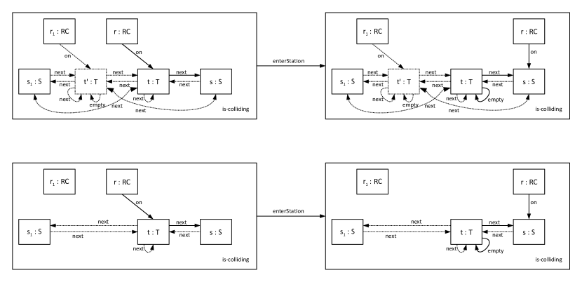
Figure 6: Applying rule $EnterStation$ on coerced shapes.

4 Soundness of Technique

Using the methods of the previous section, we can now define the set of reachable shapes of a shape graph transformation system $ST$, where $ST$ consists of a start shape graph $S_{0}$ and a set of shape production rules $(P_{i},\gamma_{i})_{i\in I}$:

$$\halign to=433.62pt{\zstrut\z@left\z@startline\ignorespaces$\@lign#$\z@stopline\hfil&\hbox to 0pt{\hss\@lign#}\cr\hbox{\hskip 0.0pt\hbox{\hbox{}\hbox{\ignorespaces\ignorespaces$reach(ST)=\mathop{\mathstrut{max}}\nolimits\left(\{S\mid S_{0}\mathrel{\lower 1.0pt\hbox{$\mathrel{-}_{\vphantom{{}}}\mkern-8.0mu\stackrel{{\scriptstyle}}{{\cleaders\hbox{$\smash{\mkern-2.0mu\mathord{-}\mkern-2.0mu}$}\hfill\vphantom{\lower 1.0pt\hbox{$\rightarrow$}}_{\vphantom{{}}}}}\mkern-11.0mu\rightarrow$}}^{*}S\}\right)$}}}\crcr}$$

Here, $\mathop{\mathstrut{max}}\nolimits$ is defined for a set of shape graphs $XS$ as in [SRW02]:

$$\halign to=433.62pt{\zstrut\z@left\z@startline\ignorespaces$\@lign#$\z@stopline\hfil&\hbox to 0pt{\hss\@lign#}\cr\hbox{\hskip 0.0pt\hbox{\hbox{}\hbox{\ignorespaces\ignorespaces$\mathop{\mathstrut{max}}\nolimits(XS):=XS\setminus\{X\mid\mathop{\mathstrut{\exists}}\nolimits X^{\prime}\in XS:X\sqsubseteq X^{\prime}\wedge X^{\prime}\not\sqsubseteq X\}$}}}\crcr}$$

The set of reachable shape graphs can be inductively constructed: we start with the initial shape graph and then successively apply the production rules. For each newly produced shape graph we check whether it can be embedded into or covers an already existing shape graph. Shape graphs that are covered by others are discarded. The following theorem states that this algorithm is sound, i.e. we do not miss any of the reachable graphs:

Theorem 4.1

Let $GT=(G_{0},(P_{i})_{i\in I})$ be a graph transformation system, $ST=(S_{0},(P_{i},\gamma_{i}))_{i\in I}))$ an associated shape transformation system with $G_{0}\sqsubseteq S_{0}$. Then

$$\halign to=433.62pt{\zstrut\z@left\z@startline\ignorespaces$\@lign#$\z@stopline\hfil&\hbox to 0pt{\hss\@lign#}\cr\hbox{\hskip 0.0pt\hbox{\hbox{}\hbox{\ignorespaces\ignorespaces$reach(GT)\subseteq\{G\mid G\text{ 2-valued }\wedge G\sqsubseteq S\wedge S\in reach(ST)\}\ .$}}}\crcr}$$

Note that due to lack of space we have left out some extra conditions here referring to coercion and the compatibility constraints used therein. The full theorem and the proof can be found in [SWW10].

At the end, we have to check for forbidden patterns in the shape graphs. A shape graph $S$ contains a forbidden pattern $\langle F,F\rangle$ ($S\models F$) if (1) there is an assignment $m$ such that $\llbracket\varphi_{F}\rrbracket_{m}^{S}\neq\mathbf{0}$, i.e. if the pattern is (potentially) present in the shape, and materialisation and coercion give us at least one valid concretisation, i.e. (2) $coerce(mat_{P}(S))\neq\varnothing$. If a forbidden pattern is not contained in a shape graph, then it is also not contained in embedded concrete graphs.

Theorem 4.2

Let $S$ be a shape graph, $\langle F,F\rangle$ a forbidden pattern, $G$ a graph such that $G\sqsubseteq S$. Then $S\not\models F\Rightarrow G\not\models F$.

In summary this shows soundness of our technique: all reachable graphs are embedded in reachable shape graphs, and if we are able to show absence of forbidden patterns in the shapes this also holds for the concrete graphs. Note that due to the overapproximation the reverse is in general not true: we might find forbidden patterns in the shapes although none of the concrete graphs contain them. Instrumentation predicates are used to reduce such situations.

Finally, a note on termination. If the algorithm is carried out as proposed above, it might not terminate although we only consider maximal shapes. This could occur if the production rules generate shapes which are all incomparable in the embedding order. To avoid this, one can introduce another abstraction step in the algorithm: Nodes which agree on all unary predicate valuations are collapsed into one. As we can only have finitely many combinations of predicate valuations this gives us finitely many different shape graphs.

5 Implementation

We implemented the verification algorithm in Java, making use of the source code of the shape analysis tool TVLA [BLARS07]. Thus we were able to take advantage of the already optimised code for logical structures provided by TVLA. Basically, our implementation loads a starting shape graph, a set of shape production rules, and a set of forbidden patterns, represented as text files each. Additionally, one needs to supply a text file listing the set of core and instrumentation predicates, the latter with their meaning formulae. The implementation then successively constructs the set of reachable shape graphs, each represented as logical structure, and checks whether a newly found shape graph contains one of the forbidden patterns. If the shape graph does contain a forbidden pattern, a counter example is generated that describes how the shape graph was constructed as sequence of production applications. Otherwise, the shape graph is added to the set of reachable shape graphs and the maximum operation is applied. If no new shape graphs can be found anymore and none of the reachable shape graphs contains a forbidden pattern, the implementation asserts that the given STS is safe.

We tested our implementation using the running example on a 3GHZ Intel Core2Duo Windows System with 3GB main memory. Our implementation needs about 250ms to verify that the running example STS is safe, i.e. no collision happens. While doing so, it temporarily constructs 108 intermediate logical structures and finds 17 logical structures in the maximised set of reachable shape graphs.

This and further case studies show that the most expensive operation in terms of runtime is the $max$ operation. We implemented it by checking for each newly found shape graph whether it can be embedded in a shape graph in the (current) set of reachable shape graph or vice versa. Thus, for each newly found shape graph we need $2n$ embedding checks, if $n$ denotes the number of shape graphs in the current set of reachable shape graphs. Furthermore, for arbitrary shape graphs checking for embedding is NP-complete ([AMSS06]). Hence it is not surprising that the $max$ operation was observed to be very costly.

6 Conclusion and Related Work

In this paper, we have introduced a shape analysis approach for generating a finite over-approximation of the reach set of a graph transformation system with infinite state space. In contrast to some of the other work done in this area, e.g. [Ren04], we derive from our strict adherence to the formalism presented in [SRW02] a very straightforward avenue for implementation, which we have demonstrated using the $3$-valued logic engine TVLA. In order to emphasize the qualities of our approach, we will now discuss how it relates to other work in this area.

In [BBKR08], a method for automatic abstraction of graphs is introduced. Intuitively, nodes are identified if their neighbourhood of radius $k\in\mathbb N$ is the same. While this automatic abstraction greatly reduces the need for human intervention in the verification process, it also reduces the flexibility of the approach. Only a certain class of systems can be handled well by neighbourhood abstraction, while our approach can be tuned to fit the needs of very different systems on a per-system basis. Furthermore, the method from [BBKR08] cannot use information from spurious counterexamples, since the abstraction leaves them with only one degree of freedom, the radius $k$. In contrast, using additional instrumentation predicates, our approach can utilise the full amount of information from spurious counterexamples.

Another approach to verifying infinite-state systems is the one by Saksena, Wibling and Jonsson [SWJ08]. It is based on backwards application of rules. By applying inverted rules to the forbidden patterns it is possible to determine whether a starting graph can lead to a failure state. The backwards application paradigm imposes some restrictions on this approach, for example forbidding the deletion of nodes and requiring a single starting pattern. Our approach does not suffer such restrictions. Furthermore, since the approach does not include an explicit abstraction and thus no information about the rest of the graph is available when applying a rule to a pattern, it would be very difficult to include concepts such as parameterised rules or parallel rule application. Since our approach uses explicit abstraction through shapes, it can encode information about the entire graph and is thus much more suited to support such extensions.

Lastly, Baldan, Corradini and König [BCK08] have written a series of papers in which they develop a unique approach to the verification of infinite state GTSs. They relate GTSs to Petri nets and construct a combined formalism, called a petri graph, on which they show certain properties via a technique called unfolding. This approach achieves many of the goals we strive for. However, a single concrete start graph is required for an analysis, which would be a major restriction in systems where there are many possible initial states, or even an unknown initial state.

The above discussion of related work is by no means exhaustive, but it suffices to show that, while each of these approaches has currently some advantages over our approach, no single approach outperforms ours in every single way. The results described in this paper lay the foundations for a new approach to the verification of infinite-state GTSs, which we strongly believe to be better suited to overcome the many problems facing any theory in this area, than the currently available approaches. As such, there are a number of limitations to our approach which we intend to tackle in the future. We plan to look at parallel rule application, negative application conditions [HHT96] and especially rules with quantifiers [Ren06] which allow to specify changes on arbitrary numbers of nodes of some particular type within one rule.

References

- [AMSS06] G. Arnold, R. Manevich, M. Sagiv, and R. Shaham. Combining shape analyses by intersecting abstractions. In In Verification, Model Checking and Abstract Interpretation (VMCAI), pages 33–48. Springer-Verlag, 2006.
- [BBKR08] J. Bauer, I. Boneva, M. E. Kurbán, and A. Rensink. A modal-logic based graph abstraction. In H. Ehrig, R. Heckel, G. Rozenberg, and G. Taentzer, editors, ICGT, volume 5214 of LNCS, pages 321–335. Springer, 2008.
- [BCC+03] A. Biere, A. Cimatti, E. Clarke, O. Strichman, and Y. Zhu. Bounded model checking. Advances in computers, 58:117–148, 2003.
- [BCK08] P. Baldan, A. Corradini, and B. König. A framework for the verification of infinite-state graph transformation systems. Inf. Comput., 206(7):869–907, 2008.
- [BLARS07] I. Bogudlov, T. Lev-Ami, T. W. Reps, and M. Sagiv. Revamping TVLA: Making Parametric Shape Analysis Competitive. In W. Damm and H. Hermanns, editors, CAV, volume 4590 of LNCS, pages 221–225. Springer, 2007.
- [CMR+97] A. Corradini, U. Montanari, F. Rossi, H. Ehrig, R. Heckel, and M. Löwe. Algebraic approaches to graph transformation - part i: Basic concepts and double pushout approach. In G. Rozenberg, editor, Handbook of Graph Grammars, pages 163–246. World Scientific, 1997.
- [HHT96] A. Habel, R. Heckel, and G. Taentzer. Graph grammars with negative application conditions. Fundam. Inform., 26(3/4):287–313, 1996.
- [Löw93] M. Löwe. Algebraic approach to single-pushout graph transformation. Theor. Comput. Sci., 109(1&2):181–224, 1993.
- [PNB04] J. L. Pfaltz, M. Nagl, and B. Böhlen, editors. AGTIVE 2003, volume 3062 of LNCS. Springer, 2004.
- [RD06] A. Rensink and D. Distefano. Abstract graph transformation. Electr. Notes Theor. Comput. Sci., 157(1):39–59, 2006.
- [Ren03] A. Rensink. The GROOVE Simulator: A Tool for State Space Generation. In Pfaltz et al. [PNB04], pages 479–485.
- [Ren04] A. Rensink. Canonical graph shapes. In D. A. Schmidt, editor, ESOP, volume 2986 of LNCS, pages 401–415. Springer, 2004.
- [Ren06] A. Rensink. Nested quantification in graph transformation rules. Graph Transformations, pages 1–13, 2006.
- [RSV04] A. Rensink, Á. Schmidt, and D. Varró. Model checking graph transformations: A comparison of two approaches. In H. Ehrig, G. Engels, F. Parisi-Presicce, and G. Rozenberg, editors, ICGT, volume 3256 of LNCS, pages 226–241. Springer, 2004.
- [SRW02] S. Sagiv, T. W. Reps, and R. Wilhelm. Parametric shape analysis via 3-valued logic. ACM Trans. Program. Lang. Syst., 24(3):217–298, 2002.
- [SV03] Á. Schmidt and D. Varró. CheckVML: A Tool for Model Checking Visual Modeling Languages. In P. Stevens, J. Whittle, and G. Booch, editors, UML, volume 2863 of LNCS, pages 92–95. Springer, 2003.
- [SWJ08] M. Saksena, O. Wibling, and B. Jonsson. Graph grammar modeling and verification of ad hoc routing protocols. In Proceedings of the Theory and practice of software, 14th international conference on Tools and algorithms for the construction and analysis of systems, pages 18–32. Springer-Verlag, 2008.
-
[SWW10]
D. Steenken, H. Wehrheim, and D. Wonisch.
Towards a shape analysis for graph transformation systems.
Technical report, University of Paderborn,
http://www.cs.uni-paderborn.de/fileadmin/Informatik/AG-Wehrheim/Personen/Dominik
Steenken/ShapeAnalysis2010TR.pdf, 2010. - [Tae03] G. Taentzer. AGG: A Graph Transformation Environment for Modeling and Validation of Software. In Pfaltz et al. [PNB04], pages 446–453.